Atomic nonaffinity as a predictor of plasticity in amorphous solids

Abstract

Structural heterogeneity of amorphous solids present difficult challenges that stymie the prediction of plastic events, which are intimately connected to their mechanical behavior. Based on a perturbation analysis of the potential energy landscape, we derive the atomic nonaffinity as an indicator with intrinsic orientation, which quantifies the contribution of an individual atom to the total nonaffine modulus of the system. We find that the atomic nonaffinity can efficiently characterize the locations of the shear transformation zones, with a predicative capacity comparable to the best indicators. More importantly, the atomic nonaffinity, combining the sign of third order derivative of energy with respect to coordinates, reveals an intrinsic softest shear orientation. By analyzing the angle between this orientation and the shear loading direction, it is possible to predict the protocol-dependent response of one shear transformation zone. Employing the new method, the distribution of orientations of shear transformation zones in model two-dimensional amorphous solids can be measured. The resulting plastic events can possibly be understood from a simple model of independent plastic events occurring at variously oriented shear transformation zones. These results shed light on the characterization and prediction of the mechanical response of amorphous solids.

Understanding how the heterogeneity of amorphous structures correlates with mechanical response remains a significant challenge. Various indicators have been proposed to quantitatively predict where the material is susceptible to plastic transformation. Some of these only consider the structural geometry, such as free volume Spaepen (1977); Zhu et al. (2017), five-fold symmetry Wakeda et al. (2007); Hu et al. (2015), and local deviation from sterically favored structures Tong and Tanaka (2018), etc. Others of these take the interaction between particles into consideration, like low-frequency normal modes Maloney and Lemaître (2004); Widmer-Cooper et al. (2008); Manning and Liu (2011); Ding et al. (2014), potential energy Shi et al. (2007), local elastic modulus Tsamados et al. (2009), flexibility volume Ding et al. (2016), mean square vibrational amplitude (MSVA) Tong and Xu (2014), local thermal energy Zylberg et al. (2017); Schwartzman-Nowik et al. (2019), local yield stress (LYS) Patinet et al. (2016); Barbot et al. (2018), and saddle points sampling Xu et al. (2018), etc. Recently, machine learning has also proven to be a promising statistical tool to build relation between structure and plastic rearrangements Schoenholz et al. (2016); Wang and Jain (2019); Bapst et al. (2020); Fan et al. (2020).

Nevertheless, most of these indicators are inherently scalar quantities while the deformation mechanism must have an oriented shear-like character Nicolas and Rottler (2018). This is clearly borne out by the fact that the orientational nature of shear transformation zones (STZs), the defects purported to be associated with plastic rearrangement, can be measured through their high sensitivity to the deformation protocol. As verified in simulations, under different loading orientations, the same glass may exhibit contrasting mechanical responses during which entirely different STZs are activated Gendelman et al. (2015); Xu et al. (2018); Zylberg et al. (2017); Patinet et al. (2016); Barbot et al. (2018).

Obtaining the mechanical response along different orientations of one STZ may be accomplished in a number of ways: by measuring the LYS Patinet et al. (2016); Barbot et al. (2018); Patinet et al. (2020), by calculating the linear response of local thermal energy with respect to strain (LRLTE) Schwartzman-Nowik et al. (2019), or by sampling low-energy events Xu et al. (2018). All of these methods require computationally expensive calculations. LYS requires prior calculations to determine the appropriate probing length scale and direct computation of response along many orientations Barbot et al. (2018). LRLTE must be recalculated under the specified mechanical load to compare different orientation Schwartzman-Nowik et al. (2019). Sampling low-energy events only captures the subset of events that are inherently viscoplastic, and requires the harvesting of large numbers of events so as to find the few lowest-energy events.

In this report, based on a perturbation analysis of the energy landscape, we derive a parameter-free and low-cost indicator, termed the atomic nonaffinity. Since this indicator is derived from a perturbation method, the atomic nonaffinity can precisely predict the mechanical behavior near the reference state and and becomes less effective as the system is deformed. We show that atomic shear nonaffinity, i.e. the shear part of the atomic nonaffinity, can efficiently predict the locations of plastic rearrangements during shear deformation of two-dimensional amorphous solids with an accuracy comparable to the best known indicators. The relevant orientational information of STZs is naturally reflected in this parameter, and analysis of the atomic shear nonaffinity indicates that the softest shear orientation of the triggered STZs aligns with the orientation of the applied shear protocol. Moreover, the distribution of orientations of activated STZs is calculated, and we show that this distribution can be understood through a simple model that assumes independent STZs with isotropically distributed soft orientations.

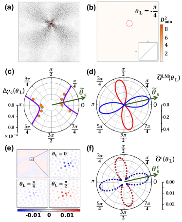
Figure 1: Analysis of configuration that was sheared to be close to the triggering of a plastic event. (a) The spatial distribution of normal mode with lowest eigenvalue. (b) The $D^{2}_{\mathrm{min}}$ field Falk and Langer (1998) after shear with strain of $\Delta\gamma=6\times 10^{-5}$ in the orientation of $\theta_{\mathrm{L}}=-\pi/4$. The inset shows the stress-strain curve. (c) The predicted triggering strain (line) and triggering strain from simulation (circles) as a function of shear angle $\theta_{\mathrm{L}}$. (d) The magnitude of nonaffine modulus contribution from the lowest mode at different $\theta_{\mathrm{L}}$. Blue line represents the range of $\theta_{\mathrm{L}}$, where the plastic event can be triggered, while the red line represents the range of $\theta_{\mathrm{L}}$, where the plastic event can not be triggered. (e) The spatial distribution of $\hat{G}(\theta_{\mathrm{L}})\cdot\mathrm{sign}(\Delta\gamma_{c}(\theta_{\mathrm{L}}))$ for different orientations. (f) The atomic shear nonaffinity in different orientations for the atom that has the maximum magnitude of atomic shear nonaffinity in (e).

To motivate the relevance of the atomic nonaffinity we first consider a special state in which a two-dimensional amorphous system is deformed to be close to the triggering strain of a plastic event via a protocol of athermal quasistatic shear. The two-dimensional glassy system, comprised of $10^{4}$ particles, was prepared via the same gradual quench and the same smoothed Lennard-Jones potential described in Ref. Barbot et al. (2018); Patinet et al. (2016). The spatial distribution of the normal mode with the lowest eigenvalue, referred to here as the lowest mode (LM), is shown in Fig. 1(a). A plastic event will be triggered in the region (Fig. S1 in the supplemental materials (SM)) where the LM is localized if the system is further sheared in this direction, denoted as the reference direction $\theta_{\text{L}}=0$. However, if the system is further sheared with similar small strains or even larger ones in other directions, such as $\theta_{\text{L}}=-\frac{\pi}{4}$ or $\frac{\pi}{4}$, the triggering of the same plastic event is not observed (Fig. 1(b) and Fig. S1 in SM). Obviously, this protocol-dependent mechanical behavior of amorphous systems cannot be clearly understood solely with scalar indicators. Here, we introduce the second and the third derivative of the energy with respect to the vibrational coordinate ($q^{*}$) of the LM, denoted as $\lambda^{*}$ and $\eta^{*}$ respectively, and the first derivative of stress of the system with respect to $q^{*}$ (denoted as $\frac{\partial\sigma_{xx}}{\partial q^{*}}$, $\frac{\partial\sigma_{yy}}{\partial q^{*}}$ and $\frac{\partial\tau_{xy}}{\partial q^{*}}$ respectively). The triggering strain for different shear orientations can be derived as (see SM for details of derivation)

$$\Delta\gamma_{c}(\theta_{\mathrm{L}})=\frac{\lambda^{*2}}{2\eta^{*}V\frac{\partial\tau(\theta_{\mathrm{L}})}{\partial q^{*}}},$$ (1)

where $V$ is the volume of the system and $\frac{\partial\tau(\theta_{\mathrm{L}})}{\partial q^{*}}$ is the first derivative of the shear stress with respect to $q^{*}$ at $\theta_{\mathrm{L}}$, which is equal to $-\frac{1}{2}(\frac{\partial\sigma_{xx}}{\partial q^{*}}-\frac{\partial\sigma_{yy}}{\partial q^{*}})\sin 2\theta_{\mathrm{L}}+\frac{\partial\tau_{xy}}{\partial q^{*}}\cos 2\theta_{\mathrm{L}}$. A similar form was also obtained from prior analyses of plastic mode Lerner (2016). Moreover, a softest shear orientation of the LM, $\tilde{\theta}_{s}$, associated with the smallest positive triggering strain can be defined as

$$\tan 2\tilde{\theta}_{s} =-\left(\frac{\frac{\partial\sigma_{xx}}{\partial q^{*}}-\frac{\partial\sigma_{yy}}{\partial q^{*}}}{\frac{2\partial\tau_{xy}}{\partial q^{*}}}\right),\text{with}$$ (2)

$$\frac{\partial\tau(\theta_{s})}{\partial q^{*}}\cdot\eta^{*} >0,\text{and}\ \theta_{s}\in(-\frac{\pi}{2},\frac{\pi}{2}].$$

Here we take the symmetry of shear into consideration and note that shear with orientation of $\theta_{s}$ is equal to shear with orientation of $\theta_{s}+\pi$. To verify the validity of the predictions of Eq. (1) and Eq. (2), further simulations were performed to directly measure $\Delta\gamma_{c}(\theta_{\text{L}})$ and $\tilde{\theta}_{s}$. As shown in Fig. 1(c), the predictions agree well with the simulation results, which suggests that the analysis of LM is successful for calculating the orientation-dependent mechanical response of the system close to the instability. When the system is far from the instability, we suppose that all the modes, especially the ones with small eigenvalues, should be taken into consideration.

To develop an indicator that takes all modes into consideration while maintaining the orientational information of each mode, we investigate how different modes contribute to the system modulus. Following Maloney Maloney and Lemaître (2004); Barron and Klein (1965), the elastic constants of amorphous solids can be derived from the second derivative of the total potential energy with respect to strain in athermal quasistatic deformation. These can be rewritten in the coordinates of eigenbasis as

$$C_{ijkl}=\frac{1}{V}\left(\frac{\partial^{2}U}{\partial\epsilon_{ij}\partial\epsilon_{kl}}+\sum_{m}\frac{\partial^{2}U}{\partial q_{m}\partial\epsilon_{ij}}\cdot\frac{dq_{m}}{d\epsilon_{kl}}\right),$$ (3)

where $U$ is the potential energy, and $q_{m}$ is the $m^{\mathrm{th}}$ coordinate of the eigenbasis of the Hessian matrix ($\frac{\partial^{2}U}{\partial r_{0i}\partial r_{0j}}$). The first term (Born term) of Eq. 3, accounts for affine displacement and is insensitive to the structural stability Cheng and Ma (2009) . The second term, containing the contribution from nonaffine relaxation in each normal mode, termed the nonaffine modulus ($\tilde{C}$) here, is sensitive to the structural stability. By expressing the stress as $\sigma_{ij}=\frac{1}{V}\frac{\partial U}{\partial\epsilon_{ij}}$ and the nonaffine “velocity” in quasistatic deformation as $\frac{dq_{m}}{d\epsilon_{kl}}=-\frac{1}{\lambda_{m}}\frac{\partial\sigma_{kl}}{\partial q_{m}}$ Maloney and Lemaître (2004), where $\lambda_{m}$ is the eigenvalue of $m^{\mathrm{th}}$ normal mode, the nonaffine part, $\tilde{C}_{ijkl}$, can be rewritten as

$$\tilde{C}_{ijkl}=\sum_{m}\tilde{C}_{ijkl,m}=\sum_{m}-\frac{V}{\lambda_{m}}\frac{\partial\sigma_{ij}}{\partial q_{m}}\frac{\partial\sigma_{kl}}{\partial q_{m}},$$ (4)

where $\tilde{C}_{ijkl,m}$ is the contribution from the $m^{th}$ normal mode, which is always negative. In shear protocols, the shear modulus is the most important elastic constant. Thus, we focus on the nonaffine shear modulus ($\tilde{G}$) and the contribution from each mode ($\tilde{G}_{m}$). The $\tilde{G}_{m}$ can be calculated by

$$\tilde{G}_{m}(\theta_{\mathrm{L}})=-\frac{V}{\lambda_{m}}\left(\frac{\partial\tau(\theta_{\mathrm{L}})}{\partial q_{m}}\right)^{2},$$ (5)

which depends on the orientation $\theta_{\mathrm{L}}$. The nonaffine shear modulus contribution of the dominant LM, $\tilde{G}^{\mathrm{LM}}$, for the state described in Fig. 1(a)-(c) is shown in Fig. 1(d). The blue line represents the orientational range, where $\Delta\gamma_{c}>0$, i.e. $\frac{\partial\tau(\theta_{\mathrm{L}})}{\partial q^{*}}\cdot\eta^{*}>0$ following Eq. 1, and the event can be triggered. The red line represents the orientational range, where the event can not be triggered. Moreover, a softest shear orientation can also be defined by the largest value of $\tilde{G}^{\mathrm{LM}}$ in the blue range which is and should be consistent with the $\tilde{\theta}_{s}$ derived from Eq. 2.

So far our results have been discussed with respect to eigenbasis. To develop an indicator expressed in terms of atomic quantities, we borrow an idea from the literature regarding the participation fraction Widmer-Cooper et al. (2008); Ding et al. (2014). By expressing the normalized eigenvector in the atomic coordinates as $\bm{\Psi}_{m}=\sum_{n,\alpha}c_{mn\alpha}\bm{e}_{n\alpha}$, where $\bm{e}_{n\alpha}$ is a unit vector corresponding to the displacement of $n^{th}$ atom in the $\alpha(=x\,\mathrm{or}\,y)$ direction, and $c_{mn\alpha}$ is the projection of the $m^{th}$ eigenvector onto $\bm{e}_{n\alpha}$, the $\tilde{C}_{ijkl}$ can be rewritten as

$$\tilde{C}_{ijkl}=\sum_{n}\hat{C}_{ijkl,n}=\sum_{n}\sum_{m,\alpha}-\frac{V}{\lambda_{m}}\frac{\partial\sigma_{ij}}{\partial q_{m}}\frac{\partial\sigma_{kl}}{\partial q_{m}}c_{mn\alpha}^{2}.$$ (6)

Here $\hat{C}_{ijkl,n}$ is the atomic nonaffinity of the $n^{th}$ atom. As most local plastic rearrangements are shear-like Argon (1979); Falk and Langer (1998), the atomic shear nonaffinity (ASN) is the most important component when investigating the STZs and can be written as

$$\hat{G}_{n}(\theta_{\mathrm{L}})=\sum_{m,\alpha}-\frac{V}{\lambda_{m}}\left(\frac{\partial\tau(\theta_{\mathrm{L}})}{\partial q_{m}}\right)^{2}c_{mn\alpha}^{2}.$$ (7)

Obviously, the value of $\hat{G}_{n}$ depends on the orientation $\theta_{\mathrm{L}}$. As a result, the spatial distribution of $\hat{G}_{n}$ in the previous case shown in Fig. 1(e) exhibits a clear orientation-dependent behavior in the region where the plastic event is located. More negative values of $\hat{G}_{n}$ mean that the corresponding atom is easier to trigger in the orientation $\theta_{\mathrm{L}}$. The $\hat{G}_{n}$ distribution calculated at different orientations indicates that $\theta_{\mathrm{L}}=0$ is the easiest shear direction for the plastic event when compared with $\theta_{\mathrm{L}}=\frac{\pi}{4}$ and $\frac{\pi}{2}$, which is consistent with the direct loading test in Fig. 1(b) and Fig. S1 in the SM. Moreover, the atom located in the core region has the maximum magnitude of atomic shear nonaffinity, denoted as $\hat{G}^{c}(\theta_{\mathrm{L}})$. Fig. 1(f) shows the $\theta_{\mathrm{L}}$-dependent $\hat{G}^{c}$, which has a similar shape as the $\tilde{G}^{\mathrm{LM}}$. This is attributed to the fact that the LM with smallest eigenvalue dominates the variation of $\hat{G}^{c}$, which can be inferred from Eq. 7. Thus, we can define the softest shear orientation for the $n^{th}$ atom as the softest shear orientation of the mode that dominates the variation of $\hat{G}_{n}$. The softest shear orientation of the $n^{\mathrm{th}}$ atom is defined as

$$\theta_{n,s}=\tilde{\theta}_{i,s},i=\mathrm{argmax}_{m}\sum_{\alpha}|\tilde{G}_{m}(\tilde{\theta}_{m,s})|c_{mn\alpha}^{2},$$ (8)

and the calculated softest shear orientation of the core atom ($\theta_{s}^{c}$) is shown in Fig. 1(f). The consistency of the proposed softest shear orientations for one STZ from the three parameters, i.e. the directly calculated triggering strain (Fig. 1(c)), nonaffine modulus of the lowest mode (Fig. 1(d)), and the atomic shear nonaffinity (Fig. 1(f)), implies that the $\theta_{s}$ defined from atomic shear nonaffinity is effective to for characterizing the orientations of STZs.

Now that we have seen the predictive capacity of atomic shear nonaffinity regarding the protocol-dependent mechanical response of a plastic event close to instability we can ask, ”What if the system is not close to instability?” and, ”How predictive is this indicator?” Predicting plastic events in an amorphous system by analyzing the local indicators of initial structure has been extensively studied in the literature Patinet et al. (2016); Ding et al. (2014); Manning and Liu (2011); Xu et al. (2018); Zylberg et al. (2017); Widmer-Cooper et al. (2008); Cubuk et al. (2015); Lerner (2016); Gendelman et al. (2015); Richard et al. (2020). To compare the reliability of local indicators for predicting plastic events, one hundred two-dimensional samples prepared with the same thermal history as the previous sample were employed for local properties calculations. The athermal quasistatic shear deformation with a strain step of $\Delta\gamma_{xy}=10^{-5}$ was then applied to each sample, and each stress drop in the stress-strain curve was associated with the resulting atomic rearrangements corresponding to one plastic event. Nonaffine rate Maloney and Lemaître (2004) was calculated for the configurations just before the stress drops, and the atom with maximum nonaffine rate was identified as the core atom, whose index is denoted as $\mathrm{ID}_{N}$ for $N^{th}$ plastic event. To compare the success of different indicators, we transform those indicators to a rank correlation (RC) value following the analysis performed by Patinet et al. Patinet et al. (2016) as

$$\mathrm{RC}_{\Psi}(n)=1-2\mathrm{CDF}_{\Psi}(n),$$ (9)

where $\Psi$ is one of the indicators, $\mathrm{CDF}_{\Psi}$ is the cumulative distribution function for the $\Psi$ of all atoms, and $\mathrm{CDF}_{\Psi}(n)$ is the function value in the range of $[0,1]$ based on the value of $\Psi$ for $n^{th}$ particle. The spatial distribution field of the calculated $\mathrm{RC}_{\hat{G}}$ with $\theta_{\mathrm{L}}=0$ is shown in Fig. 2(a). The first ten plastic events in shear protocols with $\theta_{\mathrm{L}}=0$ are almost all located at high $\mathrm{RC}_{\hat{G}}$ regions, which implies the highly predictive power of $\hat{G}$. To quantitatively compare the predictive power regarding plastic events for different local indicators, the relationship between the locations of plastic events and the corresponding values of local indicators is described by the average of $\mathrm{RC}_{\Psi}(\mathrm{ID}_{N})$ over 100 samples. The average $\mathrm{RC}_{\Psi}(\mathrm{ID}_{N})$ of investigated local indicators , such as participation fraction (PF) Manning and Liu (2011); Ding et al. (2014); Widmer-Cooper et al. (2008) in the lowest $1\%$ of normal modes, the nonaffine rate (NR) Maloney and Lemaître (2004), the MSVA Tong and Xu (2014), the LYS Patinet et al. (2016) and the ASN, are shown in Fig. 2(b). The LYS presents the highest predictive power in the early stage, since nonlinear response to shear is considered. The MSVA, and ASN shows comparable predictive power, and the other indicators have lower predictive power than those three. It is worth noting that the predicative power of the indicators depends on the stability of configurations. In the SM we show the predictive power of these indicators for configurations prepared by instantly quenching from high temperature liquids, systems in which MSVA and ASN outperform LYS. We also note that the orientational information in ASN is incomplete and it, as a modulus, has the same value for $\theta_{\mathrm{L}}=0$ and $\frac{\pi}{2}$, while local regions generally have different mechanical behavior for those two protocols.

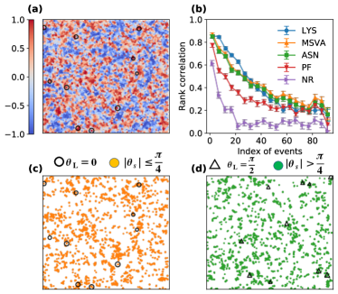
Figure 2: Predicting plastic events by analyzing initial configurations. (a) The correlation field of atomic shear nonaffinity $\hat{G}(\theta_{\mathrm{L}}=0)$ and the locations of the first ten plastic events (black circles) triggered in shear protocols with $\theta_{\mathrm{L}}=0$. (b) Correlation between the indicators including local yield stress (LYS), mean square vibrational amplitude (MSVA), atomic shear nonaffinity (ASN), participation fraction (PF), nonaffine rate (NR) with the locations of plastic events as a function of the index of the events. Averages are taken over windows of five events. Error bar at each window represents the standard deviation of the mean. (c) Orange circles represent the atoms with $\mathrm{RC}_{\hat{G}}>0$ and $|\theta_{s}|<\frac{\pi}{4}$. Black circles mark the locations of the first ten plastic events with $\theta_{\mathrm{L}}=0$. (d) Green circles represent the atoms with $\mathrm{RC}_{\hat{G}}>0$ and $|\theta_{s}|>\frac{\pi}{4}$. Triangles mark the locations of the first ten plastic events with $\theta_{\mathrm{L}}=\frac{\pi}{2}$.

As discussed in Fig. 1, we expect that the plastic events induced when shearing along direction $\theta_{\mathrm{L}}$ should be located at the atoms with $|\theta_{s}-\theta_{\mathrm{L}}|<\frac{\pi}{4}$, and here we test this expectation in one of the previous samples. We focused on the ”soft” atoms in the sample with $\mathrm{RC}_{\hat{G}}>0$, and distinguished them by the value of $\theta_{s}$. The correlation between the atom with $\mathrm{RC}_{\hat{G}}>0$ and $|\theta_{s}|<\frac{\pi}{4}$ ($|\theta_{s}|>\frac{\pi}{4}$) and the first ten plastic events of $\theta_{\mathrm{L}}=0$ ($\theta_{\mathrm{L}}=\frac{\pi}{2}$) direction is illustrated in Fig. 2(c) (Fig. 2(d)). The correlation in both Fig. 2(c) and (d) indicate that the predictive power can potentially be increased by screening for regions where the intrinsic softest orientation of $\hat{G}_{n}$ aligns with the deformation protocol. (Similar results about protocols of $\theta_{\mathrm{L}}=\frac{\pi}{4}$ and $-\frac{\pi}{4}$ are shown in SM.)

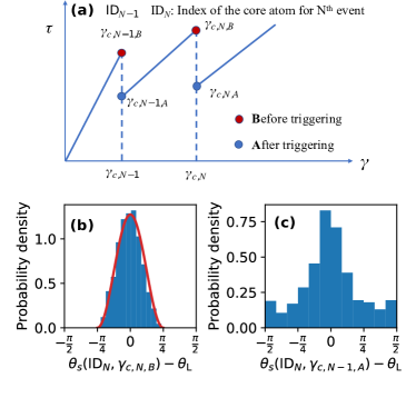
Figure 3: Ditribution of the softest shear orientations for plastic regions. (a) A schematic diagram introducing the notations used in this figure. (b) The distribution of the softest shear orientations for all the plastic events that are triggered before shear strain $0.12$ in 10 samples. The softest shear orientations are calculated based on the configuration just before each event. Red line follows the function $\frac{4}{\pi}\cos^{2}(2\Delta\theta)$. (c) Similar to (b), but the softest shear orientations for each event are calculated based on the configurations just after the previous event.

However, there still exist some number of events that are not caught by the criterion $|\theta_{s}-\theta_{\mathrm{L}}|<\frac{\pi}{4}$. This can be attributed to the rotation of $\theta_{s}$ during deformation, since the $\theta_{s}$ is calculated mainly based on a second-order perturbation method, and higher order terms and nonlinear interactions between different modes can lead to the rotation of $\theta_{s}$. To obtain the statistics of the rotation of $\theta_{s}$, the softest shear orientations of core particles of all the plastic events before shear strain $0.12$ with $\theta_{\mathrm{L}}=0$ in 10 samples are calculated based on the configurations just before each event or just after the last event (illustrated in Fig.3(a)). The distribution of the calculated $\theta_{s}$ of those core particles in the configurations just before triggering are shown in Fig. 3(b) and all $\theta_{s}$ satisfy the criterion $|\theta_{s}-\theta_{\mathrm{L}}|<\frac{\pi}{4}$, which is what we expected for systems close to instability, as discussed previously. Moreover, the peak of probability density is located at $\theta_{\mathrm{L}}$ implying that the region with the intrinsically softest orientation closest to the imposed shear orientation is easiest to trigger. However, the distribution is broadened as shown in Fig. 3(c) for the calculated $\theta_{s}^{c}$ based on the configurations just after the triggering of the previous event. In this analysis only approximately $75\%$ of the plastic events satisfy the criterion. More statistics about how orientations calculated by our perturbation method change are presented in SM. Because plastic events tend to happen at STZs closely aligned with orientation of the shear protocols, we also show that that the precision of prediction for different indicators can be improved by screening for potential STZs with the softest shear orientations in SM.

The distribution of orientations of the triggered plastic event shown in Fig. 3(b) is regular. It can be understood by a simple model of independent plastic events with intrinsic orientations. In this model, we assume that amorphous solids are isotropic and that the shear-orientation-dependent triggering strain can be derived from Eq. 1 as

$$\gamma_{c}(\theta_{\mathrm{L}})=\frac{\gamma_{c}(\theta_{s})}{\cos[2(\theta_{s}-\theta_{\mathrm{L}})]},$$ (10)

where $\theta_{s}$ is the softest shear orientation of a STZ. If we assume that the number density for a particular softest shear direction $\theta_{s}$ at different triggering strains $\gamma_{c}(\theta_{s})$ (noted as $\gamma_{c,s}$) follows a power law $\rho(\gamma_{c,s})=A\gamma_{c,s}^{\alpha}$ Karmakar et al. (2010); Hentschel et al. (2015); Lin et al. (2014a, b), the probability density distribution of orientations $\hat{\rho}(\theta_{s}-\theta_{\mathrm{L}})$ (denoted as $\hat{\rho}(\Delta\theta)$) will follow (see SM for details of derivation)

$$\hat{\rho}(\Delta\theta)=k\cos^{\alpha+1}(2\Delta\theta)$$ (11)

The probability density distribution in Fig. 3(b) corresponds to $\alpha=1$, as it closely fits a distribution function $\frac{4}{\pi}\cos^{2}(2\Delta\theta)$ (red line in Fig. 3(b)). These results are also supported by the probability distribution function of local yield stress of the samples, in which $\alpha\approx 1.1$, as shown in Ref.Patinet et al. (2016).

In summary, we have derived a general and parameter-free indicator, the atomic nonaffinity. It is well-defined and is easy to apply in systems beyond the 2d Lennard-Jones system discussed here. The atomic nonaffinity has a clear physical meaning in that the summation of atomic nonaffinities corresponds to the total nonaffine modulus of the system. The softest shear orientation of each region is defined based on the atomic shear nonaffinity and stems from anisotropy of the shear stress derivative against the coordinate of the low-frequency mode in different orientations. When combined with the sign of the third order derivative of energy with respect to coordinates, it reveals the intrinsic orientation of the plastic rearrangement and directly connects to the anisotropic mechanical response of local regions, which is important for understanding aspects of the mechanical behavior of amorphous solids not directly reflected or defined in other indicators. As atomic nonaffinity is developed based on the nonaffine response of atoms upon deformation, it naturally has a good correlation with the plastic events, comparable to the best indicators. Mechanical behavior must be correlated with structure, and we anticipate that this method will be important for elucidating the structural origin of the anisotropic mechanical response in specific systems.