Purity oscillations in coupled Bose-Einstein condensates

Abstract

Distinct oscillations of the purity of the single-particle density matrix for many-body open quantum systems have been shown to exist [Phys. Rev. A 93, 033617 (2016)]. They are found in $\mathcal{PT}$-symmetric Bose-Einstein condensates, in which the coherence of the condensate drops and is almost completely restored periodically. For this effect the presence of a gain and loss of particles turned out to be essential. We demonstrate that it can also be found in closed quantum systems of which subsystems experience a gain and loss of particles. This is shown with two different lattice setups for cold atoms, viz. a ring of six lattice sites with periodic boundary conditions and a linear chain of four lattice wells. In both cases pronounced purity oscillations are found, and it is shown that they can be made experimentally accessible via the average contrast in interference experiments. This shows that it is possible to identify this characteristic effect in closed quantum systems which have been proposed to realize $\mathcal{PT}$-symmetric quantum mechanics via separation into subsystems.

I Introduction

Today it is well established that $\mathcal{PT}$-symmetric quantum mechanics Bender and Boettcher (1998); Bender et al. (1999) can be used as an effective description of open quantum systems Moiseyev (2011). In this context complex potentials introduce a coupling to an environment which is not defined in detail. A negative imaginary part describes a decrease of the probability amplitude of a quantum particle to be in the system under consideration. In the same sense a positive imaginary potential represents an increase of this probability amplitude. $\mathcal{PT}$ symmetry of the Hamiltonian offers the possibility of balanced gain and loss, since a $\mathcal{PT}$-symmetric potential has spatially separated sinks and sources of the probability amplitude, but with the same strength. This was introduced and used in many quantum mechanical applications Znojil (1999); Mehri-Dehnavi et al. (2010); Jones and Moreira (2010); Graefe et al. (2008); Musslimani et al. (2008) as well as in quantum field theories Bender et al. (2012); Mannheim (2013); Schwarz et al. (2015); Abt et al. (2015), where a rich variety of characteristic effects of these systems, such as self-orthogonality, spontaneous $\mathcal{PT}$ symmetry breaking or quasi-Hermiticity was uncovered. However, the formalism is not restricted to quantum mechanics but also has applications in classical systems such as electromagnetic waves Bittner et al. (2012); Klaiman et al. (2008); Wiersig (2014); Bittner et al. (2014); Doppler et al. (2016) or electronic devices Schindler et al. (2011).

In optics in particular the concept of $\mathcal{PT}$ symmetry, or non-Hermitian Hamiltonians in general, has been very fruitful. Based on the fact that imaginary contributions to the refractive index can be understood as sources and sinks of the electromagnetic field amplitude El-Ganainy et al. (2007) systems of optical wave guides with balanced gain and loss were constructed and successfully proved the applicability of the theoretical formalism in experiments Rüter et al. (2010); Peng et al. (2014); Guo et al. (2009). This has led to remarkable experimental verifications such as relations to topological properties of lattice systems Weimann et al. (2017) or non-adiabatic state flips Doppler et al. (2016).

If a single particle is studied, the complex potentials act on the particle’s probability amplitude to be in the system Graefe et al. (2010). A different interpretation can be obtained in many-particle systems. For example, in the Gross-Pitaevskii equation of a Bose-Einstein condensate (BEC) the gain and loss terms in the potential modify the amplitude of the mean-field wave function, and thus describe a coherent injection or removal of particles Dast et al. (2013). In this approach the quantum system of a BEC is only discussed on the mean-field level and its quantum many-body character remains hidden.

However, the many-body properties are clearly important for the system. On the one hand it can be conjectured that quantum fluctuations make the appearance of exact $\mathcal{PT}$ symmetry impossible Schomerus (2010). On the other hand the dynamics of a condensate subject to balanced gain and loss shows a characteristic signature. As was shown Dast et al. (2016a, b) the coherence of a condensate can be affected substantially by the gain and loss effects. In the system studied in Refs. Dast et al. (2016a, b) the purity of the single-particle density matrix, which can be used as a measure of how close the condensate is to a mean-field state, drops periodically during the dynamics but is also almost completely restored in each period. This is in contradiction with the usual assumption that coherence gets lost due to interactions but never recurs.

A very fundamental study of the corresponding mechanism for the information flow in linear quantum systems is presented by Kawabata et al. Kawabata et al. (2017). Experimental studies of linear systems with respect to the available information were done in Refs. Xia et al. ; Naghiloo et al. (2019); Bian et al. .

The results of Refs. Dast et al. (2016a, b) were obtained in a many-particle description, where a master equation in Lindblad form Breuer and Petruccione (2002) was used to introduce the gain and loss of atoms. It is known that this description shows all effects visible in the Gross-Pitaevskii equation of the system and converges to its imaginary potentials in the mean-field limit of the many-body system. However, in this description the sources and drains of particles are still located in some environment, which is not specified further. Since proposals exist how $\mathcal{PT}$-symmetric BECs can be realized, we wish to investigate whether or not these realizations exhibit the purity oscillations. We suggest to exploit such possible realizations and in this work we demonstrate that purity oscillations can indeed be found and identified beyond any doubt in these systems. Since these proposals are subsystems embedded in a larger closed structure, we show here that purity oscillations can be found in closed quantum systems, which has, to the best of our knowledge, never been observed before. This renders the experimental realization of quantum systems with purity oscillations possible.

Our starting point is the proposal of Kreibich et al. Kreibich et al. (2013, 2016), which consists of a multi-well trap for the BEC. Some of the inner wells are considered as the system and the outer wells form the environment. In the mean-field limit the influx and outflux of particles into and from the system have exactly the same influence on the condensate as the imaginary potentials. A primary objective of the present work is to investigate whether such a Hermitian system, of which only a subsystem is considered, can show a behavior similar to the open system with respect to the time evolution of the coherence in the system, i.e. whether or not the purity oscillations discussed by Dast et al. Dast et al. (2016a) can occur in this Hermitian system.

To do so, we use two approaches. The first consists of a six-well setup with periodic boundary conditions. It consists basically of two coupled trimers, certainly a nontrivial system since already the isolated trimer can exhibit a rich dynamics Franzosi and Penna (2003). The second one is a chain of four wells, which is very close to the original proposal of Kreibich et al. Kreibich et al. (2013) and in which only the inner two wells are regarded as the system with gain and loss. The many-body dynamics of these systems is studied and the purity of the single particle density matrix is calculated. This will show that, as in the open system Dast et al. (2016a), due to the gain and loss of atoms in the subsystem the purity can perform oscillations, in which it drops to small values but always is nearly completely restored. As was discussed by Dast et al. Dast et al. (2016a) this effect leads to a measurable quantity in interference experiments since a high purity is necessary for a distinct average contrast in interference patters. At low values of the purity the average contrast vanishes. We confirm that this behavior is also present in our setups.

To do so, we start with a six-well system with periodic boundary conditions in Sec. II. After the preparation of the initial state (Sec. II.1) and the introduction of the calculations for the dynamics (Sec. II.2) we investigate the particle number dynamics in the single wells (Sec. II.3) and show the effect on the purity of the single-particle density matrix (Sec. II.4) as well as on the contrast in interference experiments (Sec. II.5). This is compared with the dynamics of a chain of four wells in Sec. III. Conclusions from these numerical studies are drawn in Sec. IV.

II Dynamics of condensates with periodic boundary conditions

In this section the system proposed in Fig. 1

Figure 1: Schematic representation of the setup discussed in Sec. II: Two coupled three-site subsystems forming a six-site Hermitian system.

is analyzed, with the central question under investigation as to what extent the many-particle dynamics of two coupled BECs shows a behavior similar to that of a condensate in a simple open system. A special focus is set on the time evolution of the coherence of the condensates as expressed by the purity of the single-particle density matrix.

II.1 Initial state

The situation considered is as follows. The two subsystems are initially fully separated by setting the tunneling strength $J_{2}$ to zero. At $t=0$ each subsystem is populated with a pure BEC. However, the two BECs do not share phase coherence with each other. The potential wall between the subsystems is then lowered, assigning a finite value to $J_{2}$ and inducing a dynamics in the system.

An initial state representing the situation described above can be found by proposing mean-field states for each subsystem individually, which are pure a priori. These states can be calculated with the discrete dimensionless Gross-Pitaevskii equation for three sites in the stationary case, i.e.

$$\begin{split}\mu c_{1}&=g|c_{1}|^{2}c_{1}-J_{1}c_{2}\;,\\ \mu c_{2}&=g|c_{2}|^{2}c_{2}-J_{1}c_{1}-J_{1}c_{3}\;,\\ \mu c_{3}&=g|c_{3}|^{2}c_{3}-J_{1}c_{2}\;,\end{split}$$ (1)

where $g$ represents the macroscopic particle-particle interaction and $\mu$ is the chemical potential. The ground state of this system of equations is calculated numerically under the normalization condition $|c_{1}|^{2}+|c_{2}|^{2}+|c_{3}|^{2}=\frac{1}{2}$, which ensures that the combined system is of norm one. The mean-field coefficients $c_{i}$ of the ground state can be chosen real at all sites $i$ and for the exemplary case of $g=J_{1}=1$ the calculation yields $c_{1}=c_{3}\approx 0.3604$ and $c_{2}\approx 0.4902$.

II.2 Many-particle dynamics

In general the many-particle state in the Fock base corresponding to a mean-field state is given by

$$|{\bm{c},N}\rangle=\sum\limits_{n_{1}+\cdots+n_{M}=N}\sqrt{\frac{N!}{n_{1}!\cdots n_{M}!}}\\ \times c_{1}^{n_{1}}\cdots c_{M}^{n_{M}}|{n_{1},\dots,n_{M}}\rangle\;,$$ (2)

where $N$ is the total number of particles in the system, $M$ is the number of sites and the coefficients $n_{j}$ denote the number of particles at site $j$. For our case of two independent mean-field states in two identical subsystems a direct product of two three-well states is needed with $N/2$ in each subsystem, i.e.

$$|{\psi}\rangle=|{\{c_{1},c_{2},c_{3}\},N/2}\rangle\otimes|{\{c_{4},c_{5},c_{6}\},N/2}\rangle\;.$$ (3)

The coefficients $c_{1}=c_{3}=c_{4}=c_{6}$ and $c_{2}=c_{5}$ are those calculated above.

The dynamics of the many-particle system is solved with a Bose-Hubbard type Hamiltonian

$$H=-\sum_{i,j}J_{ij}a^{\dagger}_{i}a_{j}+\frac{U}{2}\sum_{j}Ua^{\dagger}_{j}a^{\dagger}_{j}a_{j}a_{j}$$ (4)

with $J_{ji}=J_{ij}$, in which no on-site energy term is present since all wells are assumed to have the same on-site energy and dimensionless units are chosen appropriately. The operators $a_{i}^{\dagger}$ and $a_{i}$ create and annihilate a particle at site $i$, respectively. To reflect the system of Fig. 1 and to agree with the mean-field state used as initial condition we set $J_{12}=J_{23}=J_{45}=J_{56}=J_{1}$, $J_{34}=J_{61}=J_{2}$, and $U=g/(N-1)$.

II.3 Filling level dynamics

Central quantities in analyzing the dynamical behavior are the expectation values of the number operator $\langle\hat{n}_{j}\rangle=\langle\hat{a}_{j}^{\dagger}\hat{a}_{j}\rangle$ for each site (referred to as filling levels in the following). Because of the system’s symmetry that of the initial state does not get lost during the temporal evolution and there are only two independent filling levels, viz. the central levels of the subsystems ($c_{2}=c_{5}$), and all other levels ($c_{1}=c_{3}=c_{4}=c_{6}$).

By propagating the initial state with a simple Runge-Kutta algorithm the time evolution of the many-particle states is calculated for a system of $N=70$ particles. Of course the system’s dynamics depends critically on its parameters. A detailed study of the parameter dependence in the description via a master equation is given in Refs. Dast et al. (2016b, 2017). In this paper we wish to observe clear purity oscillations, and thus search for appropriate parameters. The nonlinear interaction strength $g$ and the tunneling strength within the subsystems $J_{1}$ are set to one as above and the behavior of the system is investigated for different couplings $J_{2}$ between the subsystems since this parameter induces the dynamics after the condensates have been prepared independently. In our study a value of $J_{2}=2$ turned out to provide a dynamics very similar to that of the investigation of open systems Dast et al. (2016a). An example for this choice of $J_{2}$ is shown in Fig. 2.

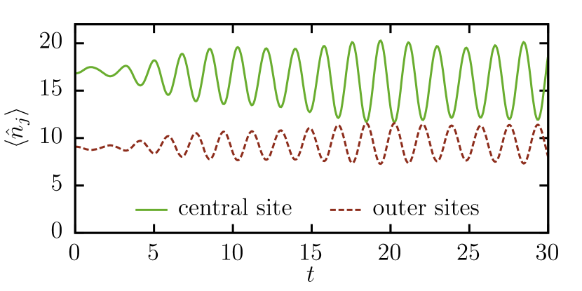
Figure 2: Time evolution of the filling levels for $N=70$, $g=J_{1}=1$ and $J_{2}=2$ for two initially fully separated BECs. Relatively stable oscillations are established after some on-set period. Due to the symmetry of the system and conservation of the total particle number, there is a phase difference of $\pi$ between the oscillations of the central site (solid line) and those of the outer sites (dashed line).

After some on-set period relatively stable oscillations are established. Due to the underlying symmetry they show a phase difference of $\pi$ between the central site of each subsystem and its outer sites. A stronger coupling of the subsystems (i.e. $J_{2}>2J_{1}$) also yields an oscillatory behavior. However, the amplitude and stability of the oscillations decrease. Larger choices of the nonlinearity $g$ result in very unstable oscillations as well.

II.4 Investigation of the purity

In accordance with the study in open systems Dast et al. (2016a) we use the purity

$$P=\frac{M}{M-1}\mathrm{tr}\,\left(\bm{\sigma}_{\mathrm{red}}^{2}\right)-\frac{1}{M-1}$$ (5)

of the reduced single-particle density matrix $\bm{\sigma}_{\mathrm{red}}$ with the elements

$$\sigma_{\mathrm{red},ij}=\frac{\langle a_{i}^{\dagger}a_{j}\rangle}{\sum_{k=1}^{M}\langle a_{k}^{\dagger}a_{k}\rangle}$$ (6)

and the dimension $M$ of the system to quantify how close the state considered is to a pure condensate. One of the subsystems corresponds to the open system of Ref. Dast et al. (2016a), and thus we use its purity $P$ with $i,j\in\{1,2,3\}$ and $M=3$. For completeness we compare it with the purity $P_{\mathrm{tot}}$ of the whole system, i.e. $P_{\mathrm{tot}}$ is calculated with $i,j\in\{1,\dots,6\}$ and $M=6$.

Since it is known that the purity oscillations are strongly related with the coupling of a system to its gain-loss environment Dast et al. (2016a, b) we investigate the purity for different strengths of the coupling of the two condensates as mediated by the tunneling constant $J_{2}$ in Fig. 3.

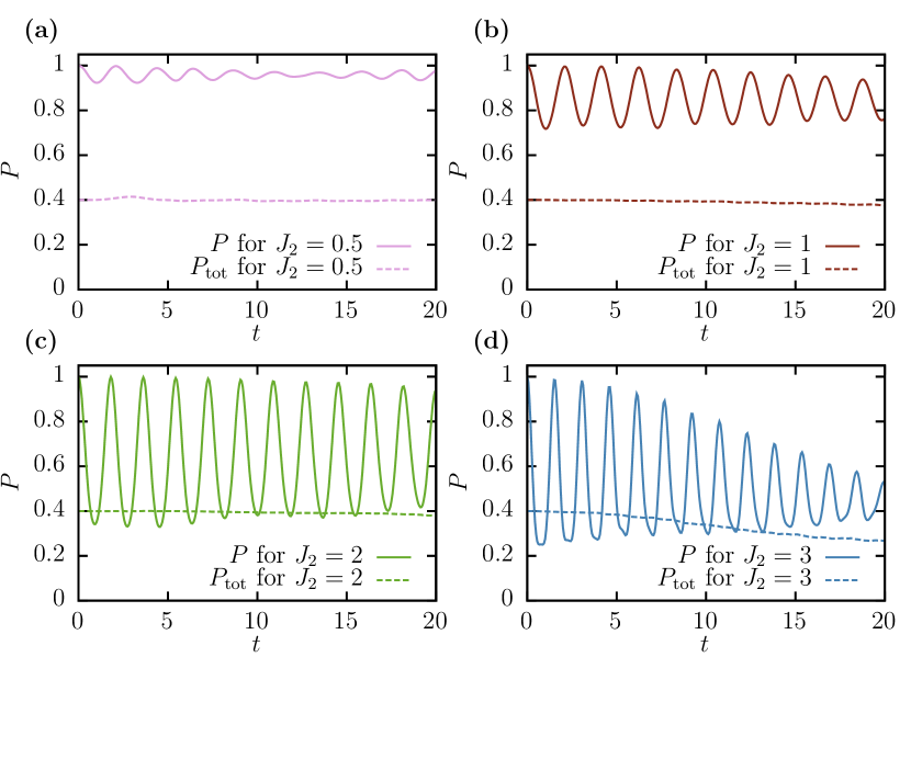
Figure 3: Time dependence of the purity $P$ (solid lines) of one subsystem and the purity $P_{\mathrm{tot}}$ (dashed lines) of the total system for different values (a) $J_{2}=0.5$, (b) $J_{2}=1$, (c) $J_{2}=2$, and (d) $J_{2}=3$ of the coupling strength between the two systems. The other parameters are $N=70$ and $g=J_{1}=1$. The purity $P$ undergoes oscillations that can be very distinct and of a large amplitude for higher values of $J_{2}$. The total purity stays almost constant at $P_{\mathrm{tot}}=0.4$ and decreases only slightly over time, which can be explained solely by statistical reasons. The amplitude and average of the oscillations of $P$ decrease over time as well, especially for the highest value of the tunneling strength $J_{2}=3$ (d).

The purity $P$ (solid lines) of one subsystem is displayed alongside the overall purity $P_{\mathrm{tot}}$ (dashed lines) of the six-site system. Since the subsystems are initially prepared in a mean-field state, i.e. with a pure condensate, all curves in the figure have to start at $P=1$ for $t=0$. As time progresses the purity does in fact undergo oscillations, whose amplitude is strongly determined by the strength of the coupling. For $J_{2}=0.5$ [Fig. 3(a)] the minimum of the first oscillation is still higher than $P=0.9$. It decreases for the stronger coupling $J_{2}=1$ [Fig. 3(b)] and reaches a value of $P\approx 0.35$ for $J_{2}=2$ [Fig. 3(c)].

Increasing the coupling even further to $J_{2}=3$ [Fig. 3(d)] does only result in a slight initial increase of the amplitude. This minimal improvement goes along with an unwanted strong overall decrease of the purity with time. In addition, the almost harmonic shape that the oscillations possess for smaller values of $J_{2}$ is lost. This is in agreement with the study of the open system Dast et al. (2016a, b), in which it was found that the purity oscillations are aligned with the particle number oscillations. In our closed system the most pronounced purity oscillations with an almost constant amplitude are achieved for the coupling strength $J_{2}=2$, which also leads to the most stable particle number oscillations.

As mentioned above, previous studies Dast et al. (2016a); Witthaut et al. (2008) found the rapid loss and subsequent restoration of the coherence to be a phenomenon of open systems, which is not possible without the coupling to an environment. In full agreement, in our case it is only possible to observe such purity oscillations by evaluating the purity for the two subsystems individually in the coupled Hermitian system presented in this paper. That is, for one subsystem the other assumes the role of the environment.

Since the initial state of the system consists of two completely separated and incoherent BECs the overall purity starts below one at $P_{\mathrm{tot}}=0.4$, which corresponds to two states with nonzero occupation of magnitude $N/2$. These are exactly the two separate mean-field states. As time progresses $P_{\mathrm{tot}}$ does not show any dynamical behavior except for a slight decrease due to statistical reasons (i.e. there are more accessible states of lower purity). An overall deterioration of the subsystem’s purity $P$ can also be observed in the long-term time evolution for the same reasons. On a long time scale the amplitude as well as the average value of the oscillations decrease.

II.5 Contrast in interference experiments

The coherence of the atoms in a BEC as measured by the purity plays a crucial role in interference experiments. As demonstrated e.g. in Ref. Andrews et al. (1997), the potential barrier between two lattice sites can be turned off, which results in an expansion of the atomic clouds of each site such that they ultimately interfere. An interference pattern can be visualized with a light source and detected using a CCD camera. For a system of low coherence these interference patterns will be different each time the interference experiment is executed because in this case there is no defined phase between the atoms of each site. However, if the system is coherent and there is a defined phase relation between the atoms of both sites, the interference pattern will be identical if the experiment is repeated under the same conditions. This behavior is expressed in the average contrast of the interference pattern. For the pattern created by the atoms of two neighboring sites $j$ and $k$ this term can be expressed in terms of the elements of the single-particle density matrix Witthaut et al. (2008),

$$\nu_{jk}=\frac{2|\!\langle\hat{a}_{j}^{\dagger}\hat{a}_{k}\rangle\!|}{\langle\hat{a}_{j}^{\dagger}\hat{a}_{j}\rangle+\langle\hat{a}_{k}^{\dagger}\hat{a}_{k}\rangle}\;\;\in\,[0,1]\;.$$ (7)

The coherence between both sites is quantified by the two-site purity

$$P_{jk}=\frac{\left(\langle\hat{a}_{j}^{\dagger}\hat{a}_{j}\rangle-\langle\hat{a}_{k}^{\dagger}\hat{a}_{k}\rangle\right)^{2}+4\langle\hat{a}_{j}^{\dagger}\hat{a}_{k}\rangle\langle\hat{a}_{k}^{\dagger}\hat{a}_{j}\rangle}{\left(\langle\hat{a}_{j}^{\dagger}\hat{a}_{j}\rangle+\langle\hat{a}_{k}^{\dagger}\hat{a}_{k}\rangle\right)^{2}}\;,$$ (8)

which is gained by considering only the matrix elements of site $j$ and $k$ in Eq. (5). Together with the squared particle imbalance

$$I_{jk}=\left(\frac{\langle\hat{a}_{j}^{\dagger}\hat{a}_{j}\rangle-\langle\hat{a}_{k}^{\dagger}\hat{a}_{k}\rangle}{\langle\hat{a}_{j}^{\dagger}\hat{a}_{j}\rangle+\langle\hat{a}_{k}^{\dagger}\hat{a}_{k}\rangle}\right)^{2}$$ (9)

this two-site purity determines the average contrast,

$$\nu_{jk}^{2}=P_{jk}-I_{jk}\;.$$ (10)

Hence, the two-site purity is equal to the squared average contrast if the filling levels are identical for both sites. In general, any finite particle imbalance lowers the average contrast while the two-site purity provides an upper limit for $\nu_{jk}^{2}$.

For a system of only two sites, as e.g. in Refs. Dast et al. (2016a, b), the abstract quantity purity of the system is thereby related to a quantity observable in experiment. Even though it is not possible to generalize this concept for multiple sites in an easy manner, it is still feasible for the system presented in this section because both outer sites of the subsystems behave identically. Thus, if a high coherence is observed between the central site and one of the outer sites, there has to be a high coherence in the subsystem as a whole.

However, for the average contrast to be largely determined by the purity, the dynamics of the particle imbalance has to play only a minor role. To explore the relationship of these quantities for the system under investigation the time evolution of the average contrast $\nu_{12}$ in an interference of sites 1 and 2 is compared in Fig. 4,

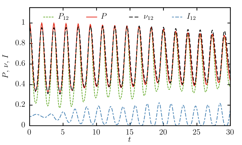
Figure 4: Average contrast $\nu_{12}$ after time $t$ in an interference experiment of sites 1 and 2 compared with the purity $P_{12}$, the squared particle imbalance $I_{12}$ of the two sites, and the overall purity of the subsystem $P$ for the same parameters as in Fig. 2. The average contrast undergoes distinct oscillations close in shape and size to those of the purities $P_{12}$ and $P$. The moderate particle imbalance is not able to disturb this behavior, partly since its minima almost coincide with the maximum of the purity.

with the particle imbalance $I_{12}$, the two-site purity $P_{12}$, and the overall purity of the subsystem $P$. Right from the start of the time evolution, while the dynamics of the filling levels are still in their on-set phase, there are already distinct oscillations of the average contrast closely related in frequency and shape to the oscillations of the purity.

Although $\nu_{12}$ is smaller than one for $t=0$ this small discrepancy caused by the finite particle imbalance does not effect the qualitative behavior. Furthermore, the maxima and minima of the evolving oscillations of $I_{12}$ almost coincide with the minima and maxima of the purity, respectively. Therefore the dynamical behavior of the particle imbalance does not compromise the alignment of the oscillations of the average contrast and the purity, but rather reinforces it. This beneficial phase relation between the purity and the particle imbalance is due to the strict symmetries of the system and cannot be expected to occur generally.

III Dynamics of condensates in a chain of four wells

Instead of the system shown in Fig. 1, one can also consider a chain of wells without periodic boundary conditions. These systems can be set up in a line, and thus can be realized in a simpler way as compared to the ring studied in the last section. However, in this case the periodic boundary conditions are lost. As we will see in the following, this is not necessarily a drawback for the observation of purity oscillations in general. We were able to identify them in a chain of six wells, built similarly to the setup shown in Fig. 1 by simply opening the chain. However, the loss of symmetry in the system leads to a more irregular dynamics. Intuitively, smaller systems with fewer degrees of freedom should show a less complicated dynamics. To put this assumption to a test, we study a chain of only four lattice sites with one condensate in the left pair of wells (subsystem 1) and another condensate in the right pair of wells (subsystem 2) as shown in Fig. 5.

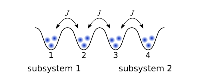
Figure 5: Schematic representation of the chain setup, in which four lattice sites are coupled. The left pair of wells forms subsystem 1 and the right pair establishes subsystem 2.

To calculate the dynamics of this system, Eq. (4) can be adapted by taking the sum over only four sites and loosing the coupling between the first and last site, which would close the ring.

As in the setup used before, the most pronounced purity oscillations are achieved for a coupling constant $J=2$ between the neighboring lattice sites. It can be intuitively understood that strong oscillations of the occupation numbers of the sites occur for high particle imbalances in the initial state. The oscillations for these parameters are shown in Fig. 6

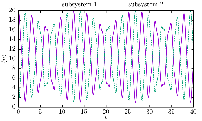
Figure 6: Particle numbers in the subsystems of the chain of four wells. The initial state consists of 20 particles in subsystem 1 and only one particle in subsystem 2. For a coupling constant $J=2$ and no particle-particle interactions ($g=0$), the dynamics of the system shows very uniform oscillations.

for the case of $g=0$, which leads to very long-lived oscillations. As can be seen they are very pronounced and still smooth enough that one can expect visible purity oscillations. Note that in the linear case the choice of the interaction strength $J$ just fixes the scale of time for given atomic parameters.

Indeed we find that, similarly to the ring of wells discussed before, the oscillations of the particle numbers correlate strongly with the observed purity oscillations. In Fig. 7

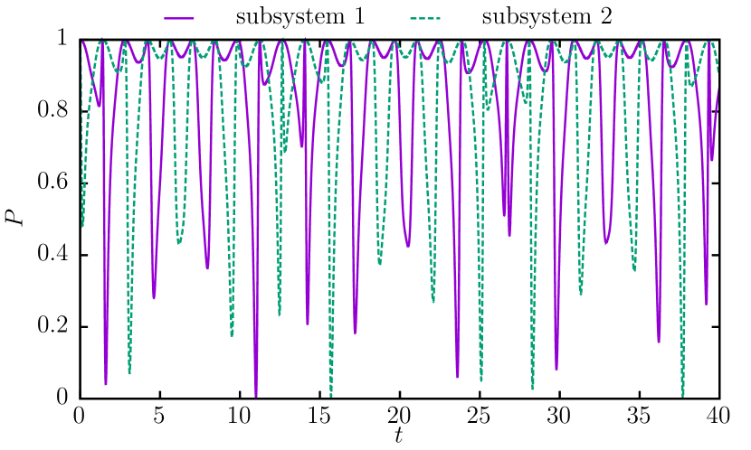
Figure 7: Purity oscillations in the two subsystems of the chain of four wells for the same parameters as in Fig. 6. The oscillations in both halfs of the system alternate with a phase shift of $\pi$.

one can see that the oscillations of the purity show large amplitudes as well. In particular, the effect that the purity is restored almost completely after it dropped survives in the system without periodic boundary conditions. Because of the large initial particle imbalance and the fact that the particles do not interact with each other ($g=0$), it is obvious that the total purity of the system remains constant at a relatively high value, which could be confirmed in our numerical calculations.

As has been shown in Sec. II.5, the purity oscillations of a system influence the average contrast $\nu$, and thus the contrast can be used to verify their existence in an experiment with atoms. In the case of our chain the contrast also shows strong oscillations, which is confirmed in Fig. 8.

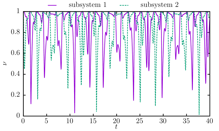
Figure 8: Average contrast in the two subsystems of the chain of four wells for the same parameters as in Fig. 6. The contrast shows a dynamic behavior similar to the purity oscillations shown in Fig. 7.

However, we observe an increasingly irregular behavior, which can be traced back to the more irregular behavior of the purity oscillations. Nevertheless the purity oscillations in a chain of four wells can still be observed by measuring the average contrast in one of the subsystems. This shows that in principle the periodic boundary conditions are not necessary, and the qualitative effect, viz. the appearance of the purity oscillations, is equivalent in both systems. The decisive reason is the gain and loss of particles in one of the subsystems. This can be achieved in a sufficiently controlled manner in both setups.

IV Conclusion

We have demonstrated the appearance of purity oscillations in two possible setups of multi-well systems for cold atoms, of which subsystems can be considered as open many-body arrangements allowing for particle exchange. One is a two-dimensional layout of six wells with periodic boundary conditions. The second is a linear chain of four wells. In both cases clear and pronounced purity oscillations are found. In contrast to the previous report Dast et al. (2016a) the gain and loss of particles is not shifted to an undefined environment but gained from a closed system and its division into subsystems.

In interference experiments the abstract purity of the single-particle density matrix becomes a quantity indirectly observable due to its clear relation to the average contrast. Because of the symmetric behavior of the outer sites in the setups used in this paper the purity becomes accessible in an interference of two neighboring sites of a subsystem. The symmetry is even such that the particle imbalance supports the oscillations of the average contrast rather than impairing it. Thus, we are convinced that one of these setups could turn out to be an experimentally feasible way of demonstrating the distinct purity oscillations predicted for balanced open quantum systems beyond the mean-field description.

References

- Bender and Boettcher (1998) C. M. Bender and S. Boettcher, Phys. Rev. Lett. 80, 5243 (1998).
- Bender et al. (1999) C. M. Bender, S. Boettcher, and P. N. Meisinger, J. Math. Phys. 40, 2201 (1999).
- Moiseyev (2011) N. Moiseyev, Non-Hermitian Quantum Mechanics (Cambridge University Press, Cambridge, 2011).
- Znojil (1999) M. Znojil, Phys. Lett. A 264, 108 (1999).
- Mehri-Dehnavi et al. (2010) H. Mehri-Dehnavi, A. Mostafazadeh, and A. Batal, J. Phys. A 43, 145301 (2010).
- Jones and Moreira (2010) H. F. Jones and E. S. Moreira, Jr, J. Phys. A 43, 055307 (2010).
- Graefe et al. (2008) E. M. Graefe, U. Günther, H. J. Korsch, and A. E. Niederle, J. Phys. A 41, 255206 (2008).
- Musslimani et al. (2008) Z. H. Musslimani, K. G. Makris, R. El-Ganainy, and D. N. Christodoulides, J. Phys. A 41, 244019 (2008).
- Bender et al. (2012) C. M. Bender, V. Branchina, and E. Messina, Phys. Rev. D 85, 085001 (2012).
- Mannheim (2013) P. D. Mannheim, Fortschr. Phys. 61, 140 (2013).
- Schwarz et al. (2015) L. Schwarz, H. Cartarius, G. Wunner, W. D. Heiss, and J. Main, Eur. Phys. J. D 69, 196 (2015).
- Abt et al. (2015) N. Abt, H. Cartarius, and G. Wunner, Int. J. Theor. Phys. 54, 4054 (2015).
- Bittner et al. (2012) S. Bittner, B. Dietz, U. Günther, H. L. Harney, M. Miski-Oglu, A. Richter, and F. Schäfer, Phys. Rev. Lett. 108, 024101 (2012).
- Klaiman et al. (2008) S. Klaiman, U. Günther, and N. Moiseyev, Phys. Rev. Lett. 101, 080402 (2008).
- Wiersig (2014) J. Wiersig, Phys. Rev. Lett. 112, 203901 (2014).
- Bittner et al. (2014) S. Bittner, B. Dietz, H. L. Harney, M. Miski-Oglu, A. Richter, and F. Schäfer, Phys. Rev. E 89, 032909 (2014).
- Doppler et al. (2016) J. Doppler, A. A. Mailybaev, J. Böhm, U. Kuhl, A. Girschik, F. Libisch, T. J. Milburn, P. Rabl, N. Moiseyev, and S. Rotter, Nature 537, 76 (2016).
- Schindler et al. (2011) J. Schindler, A. Li, M. C. Zheng, F. M. Ellis, and T. Kottos, Phys. Rev. A 84, 040101(R) (2011).
- El-Ganainy et al. (2007) R. El-Ganainy, K. G. Makris, D. N. Christodoulides, and Z. H. Musslimani, Optics Letters 32, 2632 (2007).
- Rüter et al. (2010) C. E. Rüter, K. G. Makris, R. El-Ganainy, D. N. Christodoulides, M. Segev, and D. Kip, Nat. Phys. 6, 192 (2010).
- Peng et al. (2014) B. Peng, S. K. Ozdemir, F. Lei, F. Monifi, M. Gianfreda, G. L. Long, S. Fan, F. Nori, C. M. Bender, and L. Yang, Nat. Phys. 10, 394 (2014).
- Guo et al. (2009) A. Guo, G. J. Salamo, D. Duchesne, R. Morandotti, M. Volatier-Ravat, V. Aimez, G. A. Siviloglou, and D. N. Christodoulides, Phys. Rev. Lett. 103, 093902 (2009).
- Weimann et al. (2017) S. Weimann, M. Kremer, Y. Plotnik, Y. Lumer, S. Nolte, K. G. Makris, M. Segev, M. C. Rechtsman, and A. Szameit, Nat. Mater. 16, 433 (2017).
- Graefe et al. (2010) E.-M. Graefe, H. J. Korsch, and A. E. Niederle, Phys. Rev. A 82, 013629 (2010).
- Dast et al. (2013) D. Dast, D. Haag, H. Cartarius, G. Wunner, R. Eichler, and J. Main, Fortschritte der Physik 61, 124 (2013).
- Schomerus (2010) H. Schomerus, Phys. Rev. Lett. 104, 233601 (2010).
- Dast et al. (2016a) D. Dast, D. Haag, H. Cartarius, and G. Wunner, Phys. Rev. A 93, 033617 (2016a).
- Dast et al. (2016b) D. Dast, D. Haag, H. Cartarius, J. Main, and G. Wunner, Phys. Rev. A 94, 053601 (2016b).
- Kawabata et al. (2017) K. Kawabata, Y. Ashida, and M. Ueda, Phys. Rev. Lett. 119, 190401 (2017).
- (30) L. Xia, K. Wang, X. Zhan, Z. Bian, K. Kawabata, M. Ueda, W. Yi, and P. Xue, “Observation of critical phenomena in parity-time-symmetric quantum dynamics,” Preprint arXiv:1812.01213.
- Naghiloo et al. (2019) M. Naghiloo, M. Abbasi, Y. N. Joglekar, and K. W. Murch, Nature Physics (2019), 10.1038/s41567-019-0652-z.
- (32) Z. Bian, L. Xiao, K. Wang, X. Zhan, F. A. Onaga, F. Ruzicka, W. Yi, Y. N. Joglekar, and P. Xue, “Time invariants across a fourth-order exceptional point in a parity-time-symmetric qudit,” Preprint arXiv:1903.09806.
- Breuer and Petruccione (2002) H.-P. Breuer and F. Petruccione, The Theory of Open Quantum Systems (Oxford University Press, Oxford, 2002).
- Kreibich et al. (2013) M. Kreibich, J. Main, H. Cartarius, and G. Wunner, Phys. Rev. A 87, 051601(R) (2013).
- Kreibich et al. (2016) M. Kreibich, J. Main, H. Cartarius, and G. Wunner, Phys. Rev. A 93, 023624 (2016).
- Franzosi and Penna (2003) R. Franzosi and V. Penna, Phys. Rev. E 67, 046227 (2003).
- Dast et al. (2017) D. Dast, D. Haag, H. Cartarius, J. Main, and G. Wunner, Phys. Rev. A 96, 023625 (2017).
- Witthaut et al. (2008) D. Witthaut, F. Trimborn, and S. Wimberger, Phys. Rev. Lett. 101, 200402 (2008).
- Andrews et al. (1997) M. R. Andrews, C. G. Townsend, H.-J. Miesner, D. S. Durfee, D. M. Kurn, and W. Ketterle, Science 275, 637 (1997).