Rogue waves, self-similar statistics and self-similar intermediate asymptotics
Abstract
We advance a statistical theory of extreme event emergence in random nonlinear wave systems with self-similar intermediate asymptotics. We show, within the framework of a generic D nonlinear Schrödinger equation with linear gain, that extreme events and even rogue waves in weakly nonlinear, statistical open systems emerge as parabolic-shape giant fluctuations in the self-similar asymptotic propagation regime. We analytically demonstrate the self-similar structure of the non-Gaussian statistics of emergent rogue waves and validate our results with numerical simulations. Our results shed new light on generic statistical features of extreme events in nonlinear open systems with self-similar intermediate asymptotics.
I Introduction
Rogue waves (RW), extremely rare, giant-amplitude waves obeying non-Gaussian statistics, were originally discussed in the oceanographic context Ono ; Zakh ; RW-rev . The concept has been quickly recognized as germane to generic wave supporting physics settings and RWs have been discovered, among others, in supercontinuum generating optical fibers Solli ; SCdud1 , optical cavities Res1 , Bose-Einstein condensates Blud , Raman fiber amplifiers Ham1 ; Ham2 , fiber lasers RWlas1 ; RWlas2 , laser filamentation Kasp , plasmas Mos , stimulated Raman scattering Yash1 ; Yash2 , discrete nonlinear lattices latt , and even in the multimode optical fibers and microwave transport in the linear propagation regime RWf ; Hell .
Although there apparently exists no universal mechanism describing RW generation in any physical system Dud-rev , many weakly nonlinear and dispersive statistical wave systems are governed by a generic D nonlinear Schrödinger equation (NLSE) Agra . The RW excitation in the NLSE model with random input wave fields has been studied in the anomalous dispersion regime both numerically Pic ; Dud ; Aga ; Akh1 ; Akh2 ; Sur1 ; Sur2 and experimentally Sur1 ; Sur2 . These studies revealed modulation instability driven RW excitation scenarios in weakly nonlinear conservative systems and elucidated the respective roles of spontaneous Peregrine-like breather excitation from a noisy environment and of random soliton collisions in triggering the emergence of heavy-tailed probability density distributions (PDF) of wave intensities. Such heavy-tailed PDFs herald the RW generation in the system Dud ; Sur1 ; Sur2 ; Akh1 ; Akh2 .
At the same time, open physical systems often cannot support either solitons or breathers, at least as their long-term asymptotic states, because the energy supply from—or loss to—the environment precludes the establishment of precise balance between the dispersion and nonlinearity necessary for soliton formation. Although dissipative soliton formation is possible in some open systems if, on the one hand, the nonlinearity is balanced by dispersion/diffraction and, on the other hand, gain is balanced by loss Dissol , a multitude of open systems across physics disciplines exhibit self-similar dynamics instead. Examples range from blast waves in gas dynamics and turbulent bursts in fluids Bar to nonlinear waves in optical fiber Krug1 ; Krug2 ; Ser and graded-index waveguide PSA2 ; PSA3 amplifiers, saturable two-level absorbers PSA4 , and growing Bose-Einstein condensates Drum ; Vog . Moreover, there exists a wide class of open wave systems displaying self-similar evolution in the intermediate range of parameters such that particular initial conditions at the source no longer play any role, though the system has not yet reached its steady-state Bar ; Krug1 ; Krug2 ; PSA4 ; Drum . This observation prompts a natural question: Is there an universal scenario of extreme event generation in the statistical wave systems with self-similar intermediate asymptotics? A related fundamental issue has to do with the influence of self-similar dynamics on the wave ensemble statistics in the self-similar evolution regime.
In this work, we take the first step toward addressing these fundamental topics by advancing a statistical theory of extreme events in weakly nonlinear random wave systems with unsaturated gain, described within the framework of a generic NLSE modified by a linear gain term. The modified NLSE possesses self-similar intermediate asymptotics with a parabolic intensity profile in the normal dispersion regime Krug2 . We develop a statistical theory of RW generation in the system by studying random input wave propagation there. We analytically derive and numerically verify the PDF of a wave peak power ensemble, establish its non-Gaussian statistics, and demonstrate the self-similar evolution of the ensemble statistics on random pulse propagation in the intermediate regime. We stress that, to our knowledge, this is the first demonstration of the RW statistics self-similarity in any nonlinear random wave system. Our analytical results are independent of a particular source ensemble model. In addition, they are in excellent agreement with numerical simulations of the modified NLSE.
As the NLSE with linear gain captures salient features of optical wave propagation in any weakly nonlinear amplifying media Krug1 ; Krug2 , our findings are expected to be generic. We also note that since the NLSE with a linear gain term and harmonic trapping potential attains a self-similar asymptotics as well Drum , our results apply, at least qualitatively, to optical waves in graded-index waveguide amplifiers and matter waves in growing Bose-Einstein condensates.
This work is organized as follows. In Section I, we introduce a generic dimensionless NLSE with linear gain as our mathematical model of self-similar dynamics in a wide variety of nonlinear wave systems and briefly review its parabolic self-similar solutions. In Section II, we formulate our statistical source ensemble model and present numerical results for a typical ensemble member evolution. In Section III, we present an analytical derivation of the wave peak power PDF in the self-similar regime and verify our findings with comprehensive numerical simulations of the modified NLSE. We present our conclusions in Section IV.
II Modified dimensionless nonlinear Schrödinger equation and its parabolic self-similar solutions
We consider statistical pulse propagation in a nonlinear fiber amplifier in the normal dispersion regime governed by the modified NLSE in the form
| (1) |
where is linear gain; is a group-velocity dispersion, and is a Kerr nonlinearity coefficients. To explore generic features of random waves with self-similar intermediate asymptotics, which are independent of the source and medium particulars, it will prove convenient to work with dimensionless variables, defined as
| (2) |
Here is an average pulse width and is an average peak power of a statistical input pulse ensemble; , where and are the usual nonlinear and dispersion lengths. In the dimensionless variables, the modified NLSE reads
| (3) |
where we introduced a dimensionless gain and soliton parameters which entirely determine the system dynamics given the source coherence state. We note that the smaller the soliton parameter, the faster the self-similarity is attained Krug1 .
We now present a parabolic self-similar solution to Eq. (3) by transforming the original results of Krug1 to a dimensionless form. To this end, we express the parabolic self-similar solution (similariton) in the polar form
| (4) |
where the amplitude and phase are given by the expressions
| (5) |
and
| (6) |
respectively. Henceforth we are mainly focusing on the similariton amplitude as we will derive the similariton peak power PDF; thus we ignore the phase. In Eq. (5), and are dimensionless amplitude and width of the similariton, given by
| (7) |
and
| (8) |
respectively. Here
| (9) |
where the dimensionless input pulse energy is normalized to the average energy of the input pulse ensemble,
| (10) |
Here the angle brackets denote ensemble averaging. Further, introducing the dimensionless similarity variable, , we can express the similariton profile as
| (11) |
It follows at once from Eqs. (5) through (11) that the similariton power profile has a parabolic shape which, together with its amplitude and width, is completely determined by the (scaled) input pulse energy as well as the medium gain . To study the individual pulse evolution numerically, we have to specify a random pulse ensemble at the source.
III Statistical ensemble formulation of input pulses
We now describe the input pulse ensemble in terms of a generic Gaussian Schell model MW previously employed in extreme event studies Yash1 ; Yash2 . The(GSM) ensemble has a Gaussian average intensity and Gaussian degree of the second-order temporal coherence MW ; Laleh . The GSM ensemble mutual intensity, defined as
| (12) |
reads then
| (13) |
Here is a source coherence parameter. Given , we can approximate any realistic GSM source with a finite number of (uncorrelated) excited coherent modes via the Karhunen-Loève expansion,
| (14) |
where are complex random amplitudes and are coherent mode functions, known for a GSM source to be MW
| (15) |
Here is a Hermite polynomial of the order , and we introduced the notations
| (16) |
and
| (17) |
We note that the mode functions are orthonormal such that
| (18) |
The second-order statistics of the (uncorrelated) random amplitudes are determined by
| (19) |
with the modal weight distribution,
| (20) |
The set of determines average energies of the excited coherent modes representing the source. The constant is determined by a relevant physical normalization; in our case, the (scaled) average energy of the pulse must be normalized to unity:
| (21) |
implying that
| (22) |
Note, the case implies there are no excited modes, yielding as expected; that is, only a ground mode of the source is excited—this is an example of a fully (temporarily) coherent source at the second order.
To specify the source ensemble beyond the second order, we express the set of in the polar form
| (23) |
and assume the following joint PDF of the phases and energies
| (24) |
Here is a Heaviside step function; in other words, the phases are uniformly distributed in the interval, , and the mode powers obey the Rayleigh distribution. Eq. (24) guarantees Gaussian statistics of the input pulse ensemble . We stress that coherent mode amplitude fluctuations are crucial as they determine the total source energy fluctuations, which, in turn, shape the RW statistics in the self-similar intermediate propagation regime.
We performed numerical simulations of a GSM ensemble of random pulses. In our numerical simulations we take ps, W, W-1 m-1, ps2m-1, and m-1, implying that the system is in the nonlinearity dominated regime, corresponding to the experiment Krug1 , except the average input pulse ensemble power and fiber nonlinearity are scaled by three orders of magnitude down and up, respectively. Thus, the nonlinear length remains the same and the parabolic self-similar regime is reached at sufficiently short amplifier lengths. The reason behind the scaling is practical difficulty to generate high-power (kW) ultrashort pulse sources with thermal-like power fluctuations, whereas engineering such a statistical source with the power around 1 W has been recently reported Sur1 . On the other hand, fiber amplifiers with such high nonlinearities can, in principle, be realized, for instance, by dye doping high nonlinear refractive index liquids, filling the cores of specially designed photonic crystal fibers of the kind reported in c.f. Giess ; Yash3 . Alternatively, one can attain the self-similar regime with statistical beams propagating in highly nonlinear chalcogenide planar waveguide amplifiers with defocusing nonlinearities of the order of W-1m-1 Eggl .
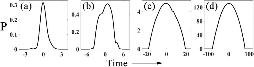
A particular ensemble realization evolution is illustrated in Fig.1. We can infer from the figure that the power profile of the realization attains a parabolic shape at the distance m; this conclusion holds for any realization, albeit the propagation distance over which the parabolic profile is reached varies from realization to realization. Most importantly, as soon as the parabolic profile is reached, it remains unchanged, up to scaling, indicating the self-similar regime ensues.
IV Self-similar statistics of peak power PDF of the pulse ensemble
The self-similar dynamics of each realization results in a remarkably simple statistical evolution of the ensemble as a whole which can be revealed by analytically deriving its peak power PDF. To this end, we can find the total energy distribution of the source pulse ensemble. As the system dynamics is entirely determined by the source energy , we derive a generic source energy PDF without committing to a specific source model under the only assumptions that (i) the mode powers have thermal-like distributions of Eq. (24) and (ii) we know the set of average mode energies . The source energy is then given by the expression
| (25) |
As all modes are uncorrelated, we can use characteristic functions to determine . To this end, we first determine a characteristic function of ,
| (26) |
It follows at once that
| (27) |
Taking an inverse Fourier transform of Eq. (27), we obtain the source energy PDF as
| (28) |
Eq. (28) can be cast into the form
| (29) |
Assuming the source modes have no degeneracy, which is certainly true of the GSM source modes, all are distinct. It follows that the integral on the r.h.s of Eq. (29) is straightforward to do in the complex plane—the result is a sum of residues at simple poles, , . The result then reads
| (30) |
Note the source energy PDF is a weighted superposition of exponential distributions of the modes carrying the average energies .
Next, let us write down the pulse peak power as
| (31) |
where we made use of Eqs. (4) through (9). The peak power PDF of the pulse ensemble is defined as
| (32) |
where the angle brackets denote averaging over an ensemble of random incident pulses. The averaging in Eq. (32) can be carried out using the delta function property,
| (33) |
Here are the two roots of the equation
| (34) |
which are written explicitly as
| (35) |
However, only the positive root is physical because . We can then drop the other root, perform a trivial integration with the delta function and, collecting all terms, we obtain a properly normalized PDF as
| (36) |
where the set of normalization constants reads
| (37) |
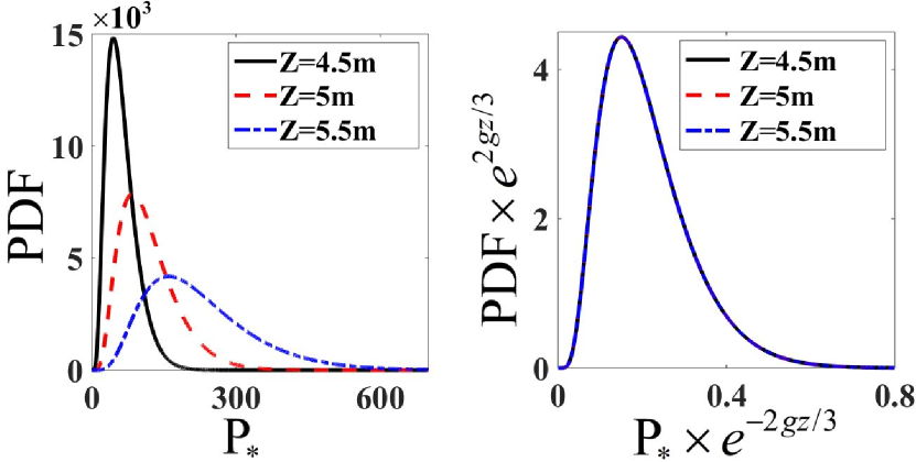
Here coherent modes can correspond to physical modes of a multimode fluctuating source. The normalization constants are found from the condition . Eq. (38) happens to represent a weighted superposition of Weibull distributions with the index Wei . Finally, we observe that the PDF can be expressed in a manifestly self-similar form as
| (38) | |||||
in terms of the similarity variable . We display the PDF in Fig 2 (left panel) at three propagation distances: , , meters in black solid, red dashed and blue dash-dotted curves, respectively. To visualize the self-similarity, we plot the PDF in the scaled variables, explicitly demonstrating in Fig. 2 (right panel) that all three curves coalesce into one. We stress that the derived self-similar structure of the PDF is independent of either a specific source model or the source coherence level, although the source coherence parameter affects the overall PDF shape as we will show below. Thus, our fundings apply to any statistical pulse ensemble with thermal-like power fluctuations in the self-similar evolution regime.
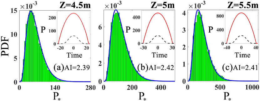
To verify our analytical results and ascertain the RW existence among the extreme events in the self-similar intermediate propagation regime, we performed numerical simulations of the modified NLSE, Eq. (3). The results are shown in Fig. 3 for the same propagation distances as in Fig.2. As is evidenced by the figure, numerical PDFs, shown by green histograms, are in excellent agreement with the theoretical curves, confirming that the system is indeed in the self-similar regime at these propagation distances. The RW emergence is marked by the abnormality index (AI) greater than two Dud-rev . The AI is defined as the ratio of an RW intensity to that of a “significant intensity” ,
| (39) |
where the “significant intensity” is defined as the mean intensity of one third of the highest peak intensity events. We can see that at all selected distances , indicating RW emergence in the system. We stress that we limit ourselves to statistical signatures of RW emergence; the examination of the other characteristic of RWs as the waves appearing from nowhere and disappearing without a trace Taki ; Akh3 lies outside the scope of this work. In the inset panels to Fig. 3 we exhibit the corresponding RWs in red curves which clearly acquire a parabolic shape. Moreover, we display the average intensity distribution of the pulse ensemble at the corresponding propagation distance in the same inset panel in a black dashed curve to show that it has a Gaussian-like rather than the parabolic shape. This is because each ensemble realization attains a parabolic shape with a different pulse width and peak pulse power, given by Eqs. (8) and (31), respectively, such that the ensemble average over these parabolic pulse profiles yields a Gaussian-like pulse. Thus, we conclude that extreme events in general—and RWs, in particular—emerge as giant parabolic shape fluctuations away from the average in the self-similar intermediate asymptotic regime. Further, we note that the AI should remain the same for a given pulse ensemble in this regime because and scale the same way with the propagation distance there. This observation is borne out by our numerical simulations displayed in Fig. 3: We can infer from the figure that up to numerical round-off errors.
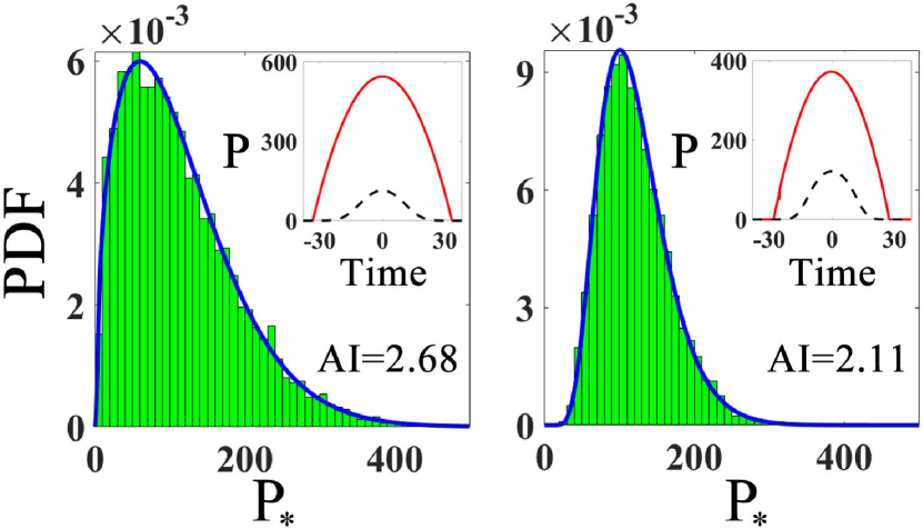
Finally, we examine the ensemble peak power PDF dependence on the source coherence state. To this end, we performed simulations for a very coherent, , and rather less coherent pulse ensembles and compared their PDFs in the self-similar asymptotic propagation regime in Fig. 4 using Eqs. (36) and (37) as well as our numerical data. We can infer from Fig. 4 by comparing either analytical PDF curves or the histograms on the left and right panels that as the source coherence increases—and so does —the PDF tail stretches as well. Indeed, for the very coherent source, while for the less coherent one in Fig. 4. This conclusion appears to be at odds with our previous results on RW generation in stimulated Raman scattering with a noisy Stokes pulse input ensemble Yash2 . To reconcile the two observations, we recall that as increases, so does the effective number of excited coherent modes of the source MW . Further, the Raman nonlinearity has very long memory implying that the greater the number of coherent modes, the greater the chances for a (giant power) “champion” mode to emerge within a Stokes pulse ensemble. This is because Raman medium memory reinforces unequal energy redistribution from a pump pulse among the Stokes pulse coherent modes throughout multiple Raman scattering cycles. In the case of weakly nonlinear amplifying media, however, the instantaneous Kerr nonlinearity has no coherent memory. Consequently, the lack of cumulative reinforcement of unequal power gain among the pulse ensemble modes favours the chances of giant power mode emergence for sources with a few excited coherent modes.
V Conclusions
In conclusion, we have elucidated the emergence scenario and salient statistical properties of extreme events in weakly nonlinear, statistical open systems exhibiting self-similar intermediate asymptotic evolution. We have demonstrated that rogue waves manifest themselves as giant self-similar fluctuations away from the average and they acquire self-similar, non-Gaussian statistics in such systems. We stress that our generic results hold in the intermediate evolution regime where gain saturation and ensuing amplified spontaneous emission noise are negligible. As the pulse intensity will have sufficiently grown up, we can no longer neglect photon emission by the excited levels of the medium atoms, stimulated by the pulse field; the stimulated emission, in turn, causes gain saturation. At the same time, spontaneously emitted photons stimulate the emission of more random photons, adding amplified spontaneous emission noise to the system. The latter, which can be the dominant noise contribution at high pulse amplification levels, is expected to ultimately lead to the break-down of the system self-similarity, cause the eventual destruction of statistically self-similar RWs and hence invalidate the proposed generic RW excitation mechanism beyond the intermediate evolution regime. The RW nature and statistical properties near gain saturation in presence of pronounced amplified spontaneous emission is a challenging open problem which we plan to address in the future.
S.A.P. acknowledges financial support from Natural Science and Engineering Research Council of Canada, (RGPIN-2018-05497); F.W. acknowledges financial support from National Natural Science Foundation of China, (11874046); Y.C. acknowledges financial support from National Natural Science Foundation of China, (91750201, 11525418).
References
- (1) M. Onorato, A. R. Osborne, M. Serio, and S. Bertone, “Freak Waves in Random Oceanic Sea States,” Phys. Rev. Lett. 86, 5831 (2001).
- (2) A. I. Dyachenko and V. E. Zaklharov, “Modulation instability of stokes wave freak wave,” JETP Lett. 81, 255 (2005).
- (3) M. Onorato, S. Residori, U. Bertolozzo, A. Montina and F. T. Arecchi, “Rogue waves and their generating mechanisms in different physical contexts,” Phys. Rep. 528, 47 (2013).
- (4) D. R. Solli, C. Ropers, P. Koonath and B. Jalali, “Optical rogue waves,” Nature (London) 450, 1054 (2007).
- (5) M. Erkintalo, G. Genty, and J. M. Dudley, “Rogue-wave-like characteristics in femtosecond supercontinuum generation,” Opt. Lett. 34, 2468 (2009).
- (6) A. Montina, U. Bortolozzo, S. Residori, and F. T. Arecchi, “Non-Gaussian statistics and extreme waves in a nonlinear optical cavity,” Phys. Rev. Lett. 103, 173901 (2009).
- (7) Y. V. Bludov, V. V. Konotop, and N. Akhmediev, “Matter rogue waves,” Phys. Rev. A 80, 33610 (2009).
- (8) K. Hammani, C. Finot, J. M. Dudley and G. Millot, “Optical rogue-wave-like extreme value fluctuations in fiber Raman amplifiers,” Opt. Express 16, 16467 (2008).
- (9) K. Hammani, A. Picozzi, and C. Finot, “Extreme statistics in Raman fiber amplifiers: From analytical description to experiments,” Opt. Commun. 284, 2594 (2011).
- (10) J. M. Soto-Crespo, Ph. Grelu, and N. Akhmediev, “Dissipative rogue waves: Extreme pulses generated by passively mode-locked lasers,” Phys. Rev. E 84, 016604, (2011).
- (11) A. F. J. Runge, N. G. R. Broderick, and M. Erkintalo, “Observation of soliton explosions in a passively mode-locked fiber laser,” Optica 2, 36 (2015).
- (12) J. Kasparian, P. Béjot, J.-P. Wolf, and J. M. Dudley, “Optical rogue wave statistics in laser filamentation,” Opt. Express 17, 12070 (2009).
- (13) W. M. Moslem, R. Sabry, S. K. El-Labany, and P. K. Shukla, “Dust-acoustic rogue waves in a nonextensive plasma,” Phys. Rev. E 84, 066402 (2011).
- (14) Y. E. Monfared and S. A. Ponomarenko, “Non-Gaussian statistics of extreme events in stimulated Raman scattering: The role of coherent memory and source noise,” Phys. Rev. A 96, 043817 (2017).
- (15) Y. E. Monfared and S. A. Ponomarenko, “Non-Gaussian statistics and optical rogue waves in stimulated Raman scattering,” Opt. Express 25, 5941 (2017).
- (16) A. Maluckov, Lj. Hadzievski, N. Lazarides, and G. P. Tsironis, “Extreme events in discrete nonlinear lattices,” Phys. Rev. E 79, 025601(R) (2009).
- (17) F. T. Arecchi, U. Bortolozzo, A. Montina, and S. Residori, ”Granularity and inhomogeneity are the joint generators of optical rogue waves,” Phys. Rev. Lett. 106, 153901 (2011).
- (18) R. Höhmann, U. Kuhl, H. J. Stöckmann, L. Kaplan, and E. J. Heller, “Freak Waves in the Linear Regime: A Microwave Study,” Phys. Rev. Lett. 104, 093901 (2010).
- (19) J. M. Dudley, F. Dias, M. Erkintalo, and G. Genty, “Instabilities, breathers and rogue waves in optics,” Nat. Photonics 8, 755 (2014).
- (20) G. P. Agrawal, Nonlinear Fiber Optics, (Academic Press, Amsterdam, 2007) 4th ed.
- (21) A. Sauter, S. Pitois, G. Millot, and A. Picozzi, “nonlinear Kerr media,” Opt. Lett. 30, 2143 (2005).
- (22) S. Toenger, T. Godin, C. Billet, F. Dias, M. Erkintalo, G. Genty, J. M. Dudley, “Emergent rogue wave structures and statistics in spontaneous modulation instability,” Sci. Rep. 5, 10380 (2015).
- (23) D. S. Agafontsev and V. E. Zakharov, “Integrable turbulence and formation of rogue waves,” Nonlinearity 28, 2791 (2015).
- (24) J. M. Soto-Crespo, N. Devine, and N. Akhmediev, “Integrable Turbulence and Rogue Waves: Breathers or Solitons?” Phys. Rev. Lett. 116, 103901 (2016).
- (25) N. Akhmediev, J. M. Soto-Crespo, and N. Devine, “Breather turbulence versus soliton turbulence: Rogue waves, probability density functions, and spectral features,” Phys. Rev. E 94, 022212 (2016).
- (26) P. Walczak, S. Randoux, and P. Suret, “Optical Rogue Waves in Integrable Turbulence,” Phys. Rev. Lett. 114, 143903 (2015).
- (27) P. Suret, R. El Koussaifi, A. Tikan, C. Evain, S. Randoux, C. Szwaj, and S. Bielawski, ”Single-shot observation of optical rogue waves in integrable turbulence using time microscopy,” Nat. Commun. 7, 13136 (2016).
- (28) N. Akhmediev and A. Ankiewicz, Dissipative Solitons, Lecture Notes in Physics (Springer, Berlin, 2005).
- (29) G. I. Barenblatt, Scaling, Self-Similarity, and Intermediate Asymptotics, (Cambridge Univ. Press, Cambridge, 1996).
- (30) M. E. Fermann, V. I. Kruglov, B. C. Thomsen, J. M. Dudley, and J. D. Harvey, “Self-Similar Propagation and Amplification of Parabolic Pulses in Optical Fibers,” Phys. Rev. Lett. 84, 6010 (2000).
- (31) V. I. Kruglov and J. D. Harvey, “Asymptotically exact parabolic solutions of the generalized nonlinear Schrödinger equation with varying parameters,” J. Opt. Soc. Am. B 23, 2541 (2006).
- (32) V. N. Serkin and A. Hasegawa, “Exactly integrable nonlinear Schrödinger equation models with varying dispersion, nonlinearity and gain: application for soliton dispersion,” IEEE J. Sel. Top. Quant. Electron. 8, 418 (2002).
- (33) S. A. Ponomarenko and G. P. Agrawal, “Do Solitonlike Self-Similar Waves Exist in Nonlinear Optical Media?” Phys. Rev. Lett. 97, 013901 (2006).
- (34) S. A. Ponomarenko and G. P. Agrawal, “Optical similaritons in nonlinear waveguides,” Opt. Lett. 32,1659 (2007).
- (35) S. A. Ponomarenko and S. Haghgoo, “Self-similarity and optical kinks in resonant nonlinear media,” Phys. Rev. A 82 051801(R) (2010).
- (36) P. D. Drummond and K. V. Kheruntsyan, “Asymptotic solutions to the Gross-Pitaevskii gain equation: Growth of a Bose-Einstein condensate,” Phys. Rev. A 63, 013605 (2000).
- (37) B. Kneer, T. Wong, K. Vogel, W. P. Schleich, and D. F. Walls, “Generic model of an atom laser,” Phys. Rev. A 58, 4841 (1998).
- (38) R. Zhang, J. Teipel, and H. Giessen, “Theoretical design of a liquid-core photonic crystal fiber for supercontinuum generation,” Opt. Express 14, 6800 (2006).
- (39) Y. E. Monfared and S. A. Ponomarenko, “Extremely nonlinear carbon-disulfide-filled photonic crystal fiber with controllable dispersion,” Opt. Mat. 88, 406, (2019).
- (40) M. Lamont, B. Luther-Davies, D-Y. Choi, S. Madden and B. J. Eggleton, “Supercontinuum generation in dispersion engineered highly nonlinear ( = 10 /W/m) chalcogenide planar waveguide,” Opt. Express 16, 14938 (2008).
- (41) L. Mandel and E. Wolf, Optical Coherence and Quantum Optics (Cambridge University Press, Cambridge, 1995).
- (42) L. Mokhtarpour and S. A. Ponomarenko, “Fluctuating pulse propagation in resonant nonlinear media: self-induced transparency random phase soliton formation,” Opt. Express 23, 30270 (2015).
- (43) W. A. Weibul, “A Statistical Distribution Function of Wide Applicability,” J. Appl. Mech. 18, 293 (1951).
- (44) N. Akhmediev, A. Ankiewicz, and M. Taki, “Waves that appear from nowhere and disappear without a trace,” Phys. Lett. A 373, 675, (2009).
- (45) N. Akhmediev, J-M. Soto-Crespo, and A. Ankiewicz, “Extreme waves that appear from nowhere: On the nature of rogue waves,” Phys. Lett. A 373, 2137 (2009).