GAT: Generative Adversarial Training for Adversarial Example Detection and Robust Classification
Abstract
The vulnerabilities of deep neural networks against adversarial examples have become a significant concern for deploying these models in sensitive domains. Devising a definitive defense against such attacks is proven to be challenging, and the methods relying on detecting adversarial samples are only valid when the attacker is oblivious to the detection mechanism. In this paper we propose a principled adversarial example detection method that can withstand norm-constrained white-box attacks. Inspired by one-versus-the-rest classification, in a K class classification problem, we train K binary classifiers where the i-th binary classifier is used to distinguish between clean data of class i and adversarially perturbed samples of other classes. At test time, we first use a trained classifier to get the predicted label (say k) of the input, and then use the k-th binary classifier to determine whether the input is a clean sample (of class k) or an adversarially perturbed example (of other classes). We further devise a generative approach to detecting/classifying adversarial examples by interpreting each binary classifier as an unnormalized density model of the class-conditional data. We provide comprehensive evaluation of the above adversarial example detection/classification methods, and demonstrate their competitive performances and compelling properties. Code is available at https://github.com/xuwangyin/GAT-Generative-Adversarial-Training 111A thorough evaluation of the proposed method is available at Tramer et al. (2020)..
1 Introduction
Deep neural networks have become the staple of modern machine learning pipelines, achieving state-of-the-art performance on extremely difficult tasks in various applications such as computer vision (He et al., 2016), speech recognition (Amodei et al., 2016), machine translation (Vaswani et al., 2017), robotics (Levine et al., 2016), and biomedical image analysis (Shen et al., 2017). Despite their outstanding performance, these networks are shown to be vulnerable against various types of adversarial attacks, including evasion attacks (aka, inference or perturbation attacks) (Szegedy et al., 2013; Goodfellow et al., 2014; Carlini & Wagner, 2017b; Su et al., 2019) and poisoning attacks (Liu et al., 2017; Shafahi et al., 2018). These vulnerabilities in deep neural networks hinder their deployment in sensitive domains including, but not limited to, health care, finances, autonomous driving, and defense-related applications and have become a major security concern.
Due to the mentioned vulnerabilities, there has been a recent surge toward designing defense mechanisms against adversarial attacks (Gu & Rigazio, 2014; Jin et al., 2015; Papernot et al., 2016b; Bastani et al., 2016; Madry et al., 2017; Sinha et al., 2018), which has in turn motivated the design of stronger attacks that defeat the proposed defenses (Goodfellow et al., 2014; Kurakin et al., 2016b; a; Carlini & Wagner, 2017b; Xiao et al., 2018; Athalye et al., 2018; Chen et al., 2018; He et al., 2018). Besides, the proposed defenses have been shown to be limited and often not effective and easy to overcome (Athalye et al., 2018). Alternatively, a large body of work has focused on detection of adversarial examples (Bhagoji et al., 2017; Feinman et al., 2017; Gong et al., 2017; Grosse et al., 2017; Metzen et al., 2017; Hendrycks & Gimpel, 2017; Li & Li, 2017; Xu et al., 2017; Pang et al., 2018; Roth et al., 2019; Bahat et al., 2019; Ma et al., 2018; Zheng & Hong, 2018; Tian et al., 2018). While training robust classifiers focuses on maintaining performance in presence of adversarial examples, adversarial detection only cares for detecting such examples.
The majority of the current detection mechanisms focus on non-adaptive threats, for which the attacks are not specifically tuned/tailored to bypass the detection mechanism, and the attacker is oblivious to the detection mechanism. In fact, Carlini & Wagner (2017a) and Athalye et al. (2018) showed that the detection methods presented in (Bhagoji et al., 2017; Feinman et al., 2017; Gong et al., 2017; Grosse et al., 2017; Metzen et al., 2017; Hendrycks & Gimpel, 2017; Li & Li, 2017; Ma et al., 2018), are significantly less effective than their claims under adaptive attacks. Overall, current solutions are mostly heuristic approaches that cannot provide performance guarantees.
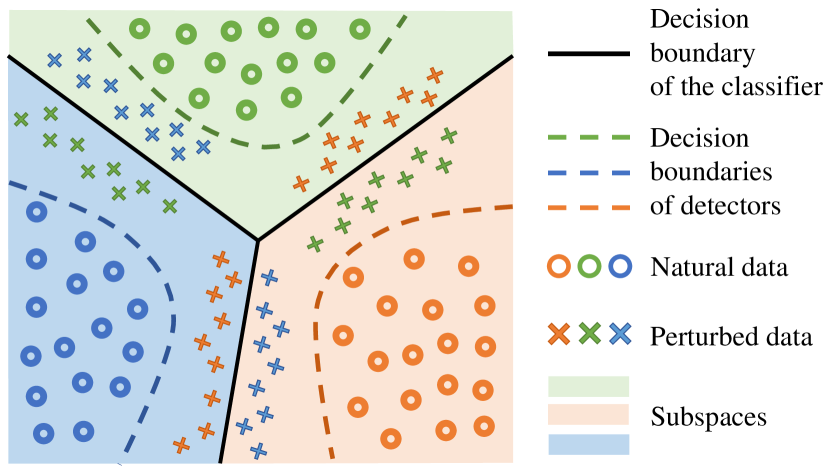
In this paper we propose a detection mechanism that can withstand adaptive attacks. The idea is to partition the input space into subspaces based on the original classifier’s decision boundary, and then perform clean/adversarial example classification the subspaces. The binary classifier in each subspace is trained to distinguish in-class samples from adversarially perturbed samples of other classes. At inference time, we first use the original classifier to get an input sample’s predicted label , and then use the -th binary classifier to identify whether the input is a clean sample (of class ) or an adversarially perturbed sample (of other classes). Fig. 1 provides a schematic illustration of the proposed approach.
Our specific contributions are: (1) We develop a principled adversarial example detection method that can withstand adaptive attacks. Empirically, our best models improve previous state-of-the-art mean distortion from 3.68 to 5.65 on MNIST dataset, and from 1.1 to 1.5 on CIFAR10 dataset. (2) We study powerful and versatile generative classification models derived from our detection framework and demonstrate their competitive performances over discriminative robust classifiers. While discriminative robust classifiers are vulnerable to rubbish examples, inputs that have confident predictions under our models have interpretable features.
2 Related works
Adversarial attacks Since the pioneering work of Szegedy et al. (2013), a large body of work has focused on designing algorithms that achieve successful attacks on neural networks (Goodfellow et al., 2014; Moosavi-Dezfooli et al., 2016; Kurakin et al., 2016b; Chen et al., 2018; Papernot et al., 2016a; Carlini & Wagner, 2017b). More recently, iterative projected gradient descent (PGD), has been empirically identified as the most effective approach for performing norm constrained attacks, and the attack reasonably approximates the optimal attack (Madry et al., 2017).
Adversarial example detection The majority of the methods developed for detecting adversarial attacks are based on the following core idea: given a trained -class classifier, , and its corresponding clean training samples, , generate a set of adversarially attacked samples , and devise a mechanism to discriminate from . For instance, Gong et al. (2017) use this exact idea and learn a binary classifier to distinguish the clean and adversarially perturbed sets. Similarly, Grosse et al. (2017) append a new “attacked” class to the classifier, , and re-train a secured network that classifies clean images, , into the classes and all attacked images, , to the -th class. In contrast to Gong et al. (2017); Grosse et al. (2017), which aim at detecting adversarial examples directly from the image content, Metzen et al. (2017) trained a binary classifier that receives as input the intermediate layer features extracted from the classifier network , and distinguished from based on such input features. More importantly, Metzen et al. (2017) considered the so-called case of adaptive/dynamic adversary and proposed to harden the detector against such attacks using a similar adversarial training approach as in Goodfellow et al. (2014). Unfortunately, the mentioned detection methods are significantly less effective under an adaptive adversary equipped with a strong attack (Carlini & Wagner, 2017a; Athalye et al., 2018).
3 Proposed Approach to Detecting Adversarial Examples
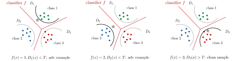
The proposed approach to detecting adversarial examples is based on the following simple idea. Assume there is an input sample , and it is predicted as by the classifier , then is either a true sample of class (assuming no misclassification) or an adversarially perturbed sample of other classes. To determine which is the case we can use a binary classifier that is specifically trained to distinguish between clean samples of class and adversarially perturbed samples of other classes. Because can be any one of the class, we need to train a total of binary classifier in order to have a complete solution. Fig. 2 provides a schematic illustration of the above detection idea. We next provide a mathematical justification and more details about how to train the detection model.
In a ) class classification problem, given a dataset of clean samples , along with labels , let be a classifier on , and be a set of -norm bounded adversarial examples computed from : , . We use and to respectively denote the clean samples and adversarial examples which are predicted by as class . Let , where is a binary classifier trained to distinguish between samples from (assigned as class 1) and samples from (assigned as class 0). We use to model and predict when and when . Consider the following procedure to determine whether a sample is an adversarial example (i.e., whether it comes from or ):
First obtain the estimated class label , then use the -th binary classifier to predict: if then categorize as a clean sample, otherwise categorize it as an adversarial example.
This algorithm can be viewed as a binary classifier, and its accuracy is given by
| (1) |
Crucially, because the errors of individual binary classifiers are independent, maximizing Eq. 1 is equivalent to optimizing the performances of individual binary classifiers. solves the binary classification problem of distinguishing between samples from and samples from , and therefore can be trained with a binary classification objective:
| (2) |
where is a loss function that measures the discrepancy between ’s output and the supplied label (e.g., the negative log likelihood loss). In order to harden against adaptive attacks, we follow Madry et al. (2017) and incorporate the adversary into the training objective:
| (3) |
where , and we assume that is large enough such that .
The equality constraint in Eq. 3 complicates the inner maximization. We observe that by dropping this constrain we have the following upper bound of the first loss term:
Because we are minimizing , we can instead minimizing this upper bound, which gives us the unconstrained objective
| (4) |
We can further simply this objective by using the fact that when is used as the training set, can overfit on such that and are respectively good approximations of and :
| (5) |
In words, each binary classifier is trained using clean samples of a particular class and adversarial examples (with respect to ) created from samples of other class. The inner maximization is solved using the PGD attack (Madry et al., 2017). We use the negative log likelihood loss as and minimize it using gradient-based optimization methods.
From a classification point of view, we can reformulate the above detection algorithm as a classifier that has a rejection option: given input and its prediction label , if , then is rejected, otherwise it’s classified as . We will refer to this classification model as an integrated classifier.
3.1 A Generative approach to adversarial example detection/classification
The proposed approach makes use of a trained classifier to get the predicted label, but is not strictly necessary: we can use in place of to do classification.
We can interpret as an one-versus-the-rest (OVR) classifier. In a class classification problem, a OVR classifier consists of binary classifiers, with each one trained to solve a two-class problem of separating samples in a particular class from samples not in that class. differs from a traditional OVR classifier in that is trained to distinguish between samples in class and adversarially perturbed samples of other classes, but because the loss on adversarial inputs is an upper bound of the loss on clean samples, the binary classifier should also be able to separate samples of class from clean samples of other classes. When is viewed as an OVR classifier, the classification rule is
| (6) |
We can also interpret as a generative classifier. Our experiments show that has a strong generative property: performing adversarial attacks on causes visual features of class to appear in the attacked data (in some cases, the attacked data become a valid instance of class ). Although a similar phenomenon is observed in standard adversarial training (Tsipras et al., 2018; Engstrom et al., 2019; Santurkar et al., 2019), the generative property of our model seems to be much stronger than that of a softmax adversarially robust classier (Fig. 4, Fig. 6, and Fig. 7). These results motivate us to reinterpret as an unnormalized density model (i.e., an energy-based model (LeCun et al., 2006)) of the class- data. This interpretation allows us to obtain the class-conditional probability of an input by:
| (7) |
where , with being the logit output of , and
| (8) |
is an intractable normalizing constant known as the partition function. We can then apply the Bayes classification rule to obtain a generative classifier:
| (9) |
where we have assumed all partition functions and class priors to be equal. Because we explicitly model , we can use this quantity to reject low probability inputs which can be any samples that do not belong to class . In this work we focus on the scenario where low probability inputs are adversarially perturbed samples of other classes and the rejected samples are considered as adversarial examples. Because is computed by applying the logistic sigmoid function to , and the logistic sigmoid function is a monotonically increasing function of its argument, the generative classifier (Eq. 9) is equivalent to the OVR classifier (Eq. 6).
In the following sections, we will use integrated detection to refer to the original detection approach where we make use an extra classifier , and generative detection to refer to this alternative approach where we first use the generative classifier Eq. 9 to get the predicted label of an input , and then use to determine whether is adversarial input.
4 Evaluation methodology
4.1 Robustness test
We first validate the robustness of individual binary classifiers by following the standard methodology for robustness testing: we train the binary classifier with PGD attack configured with a particular combination of step-size and number of steps, and then test the binary classifier’s performance under PGD attacks configured with different combinations of step-sizes and number of steps. We use AUC (area under the ROC Curve) as the detection performance metric. AUC is an aggregated measurement of detection performance across a range of thresholds, and can be interpreted as the probability that the binary classifier assigns a higher score to a random positive sample than to a random negative example. For a given , the AUC is computed on the set , where .
4.2 Adversarial Example Detection Performance
Having validated the robustness of individual binary classifier, we evaluate the overall performance of the proposed approach to detecting adversarial examples. According to the detection algorithm, we first obtain the predicted label , and then use the -th binary classifier’s logit output to predict: if , then is a clean sample, otherwise it is an adversarially perturbed sample.
We use to denote the test set that contains clean samples, and to denote the corresponding perturbed test set. For a given , we compute the true positive rate (TPR) on and false positive rate (FPR) on (here, clean samples are in the positive class). These two metrics are respectively defined as
| (10) |
and
| (11) |
We observe that for the norm ball constraint we considered in the experiments, not all perturbed samples can cause misclassification on , so we use in the FPR definition to constrain that only adversarial inputs that actually cause misclassification can be counted as false positives.
Given a clean sample and its groundtruth label , we consider three approaches to creating the corresponding adversarial example . Here we will focus on untargeted attacks.
Classifier attack This attack corresponds to the scenario where the adversary is oblivious to the detection mechanism. Inspired by the CW attack (Carlini & Wagner, 2017b), the adversarial example is computed by minimizing,
| (12) |
where is the classifier’s logit outputs.
Detector attack In this scenario adversarial examples are produced by attacking only the detector. We first construct a detection function by aggregating the logit outputs of individual binary classifiers:
| (13) |
The adversarial example is then computed by minimizing
| (14) |
According to our detection rule, a low value of a binary classifier’s logit output indicates the detection of an adversarial example, and therefore by minimizing the negative of the logit output we make the adversarial input harder to detect. can also be used with the CW loss Eq. 12 or the cross-entropy loss, but we find the attack based on Eq. 14 to be most effective.
Combined attack The combined attack is an adaptive method that considers both the classifier and the detector. We consider two loss functions for the combined attack. The first is based on the adaptive attack of Carlini & Wagner (2017a) which has been shown to be effective against existing detection methods. We first construct a new detection function with Eq. 13 and then use ’s largest logit output (low value of this quantity indicates detection of an adversarial example) and the classifier logit outputs to construct a new classifier :
| (15) |
The adversarial example is then computed by minimizing the loss function
| (16) |
In practice we observe that the optimization of Eq. 16 tends to stuck at the point where keeps changing signs while staying as a large negative number (which indicates detection). In light of the above issues we derive a more effective attack by combining Eq. 12 and Eq. 14:
| (17) |
In words, if is not yet an adversarial example on (case 1), optimize it for that goal, otherwise optimize it for evading the detection (case 2).
We note that the above three attacks are for the original detection approach (i.e., integrated detection). The generative detection approach (Section 3.1) does not make use of and we use Eq. 14 to create adversarial examples for generative detection.
4.3 Robust Classification Performance
In robust classification, the accuracy of a softmax robust classifier is evaluated on the original test test (the standard accuracy) and the adversarially perturbed test set (the robust accuracy). Because the generative classifier comes with the reject option, we use slightly different metrics. On the clean test dataset , we define the standard accuracy as the fraction of samples that are correctly classified () and at the same time not rejected ():
| (18) |
In the adversarially perturbed test dataset , we will consider a data sample as properly handled when it is rejected (), regardless of whether it causes misclassification. In this way, only misclassified () and unrejected () samples are counted as errors:
| (19) |
To compare different classifiers under the same metrics, we compute the error of a softmax robust classifier on as
| (20) |
We respectively use Eq. 17 and Eq. 14 to compute the for the integrated classifier and the generative classifier.
5 Experiments
5.1 MNIST
We train four detection models (each consists of ten binary classifiers) by using different combinations of p-norm and perturbation limit (Table 5). The adversarial examples used for training and validation are computed using PGD attacks of different steps and step sizes (Table 5). At each step of PGD attack we use the Adam optimizer to perform gradient descent, both for -based and -based attacks. Appendix A.1 provides more training details.
Robustness results Table 1 and Table 7 show that and are able to withstand PGD attacks configured with different steps and step-size, for both -based and -based attacks. The binary classifiers also exhibit robustness when the attack uses -norm or perturbation limit that are different from those used for training the model (Table 8). The models are also robust when the attacks use multiple random restarts (Table 9).
| PGD attack steps, step size | model | model | ||
|---|---|---|---|---|
| 200, 0.01 | 0.99959 | 0.99971 | 0.99830 | 0.99869 |
| 2000, 0.005 | 0.99958 | 0.99971 | 0.99796 | 0.99861 |
| PGD attack steps, step size | model | model | ||
|---|---|---|---|---|
| 200, 0.1 | 0.99962 | 0.99968 | 0.99578 | 0.99987 |
| 2000, 0.05 | 0.99927 | 0.99900 | 0.99529 | 0.99918 |
| Detection method | Mean distortion |
|---|---|
| State-of-the-art (Carlini & Wagner, 2017a) | 3.68 |
| Ours (generative detection with binary classifiers) | 4.40 |
| Ours (generative detection with binary classifiers) | 5.65 |
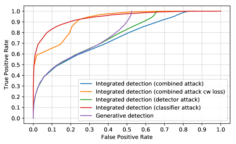
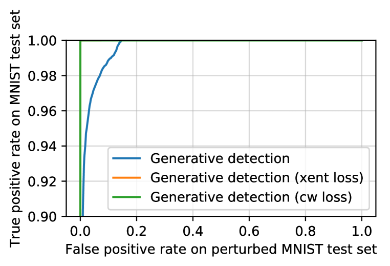
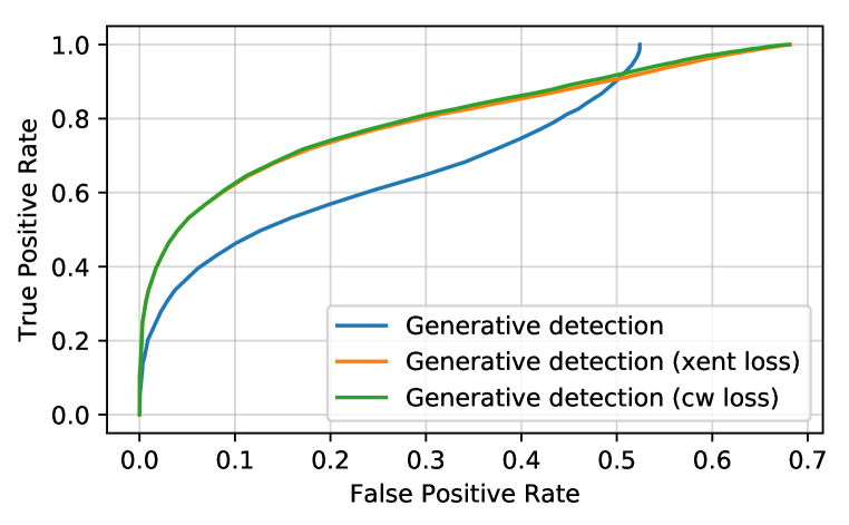
Detection results Fig. 3(a) shows the performances of integrated detection and generative detection under different attacks. Combined attack with Eq. 17 is the most effective attack against integrated detection, and is much more effective than the combined attack with Eq. 16. Overall, generative detection outperforms integrated detection when they are evaluated under their respective most effective attack. It is also interesting to note that when the adversarial examples are created by attacking only the classifier (Eq. 12), integrated detection is able to perfectly detect these adversarial examples (see the red curve that overlaps the y-axis).
Given that generative detection is the most effective approach among the proposed approaches, we compare it with state-of-the-art detection methods (Carlini & Wagner, 2017a). Table 2 shows that generative detection outperforms the state-of-the-art method by large margins. Appendix B provides details about how the mean distortions are computed.
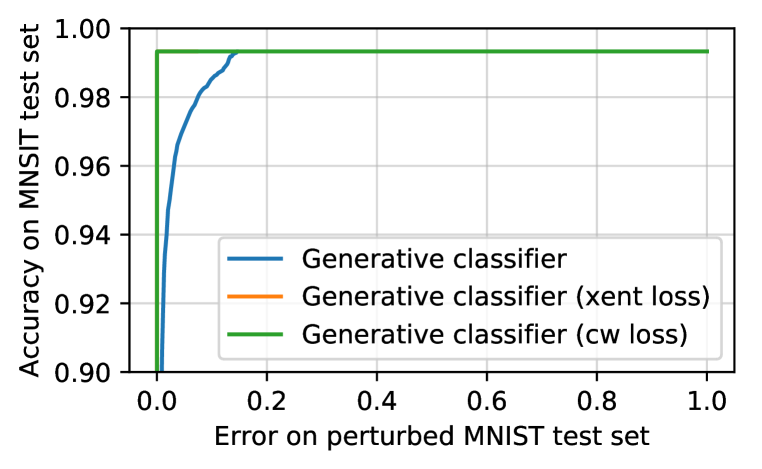
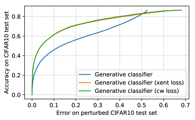
Classification results Figure 3(b) shows the standard and robust classification performances of the proposed classifiers and a state-of-the-art softmax robust classifier (Madry et al., 2017). Our models provide the reject option that allows the user to find a balance between standard accuracy and robust error by adjusting the rejection threshold. We observe that a stronger attack () breaks the softmax robust classifier (as indicated by the right red cross), while the generative classifier still exhibits robustness, even though both models are trained with the constraint.
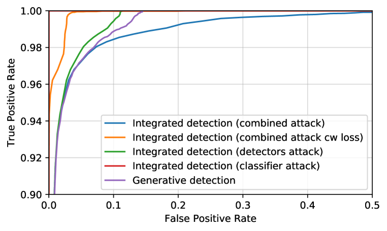
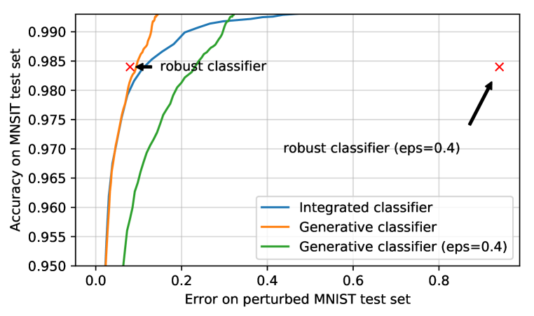
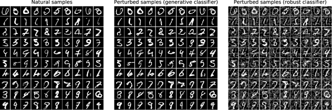
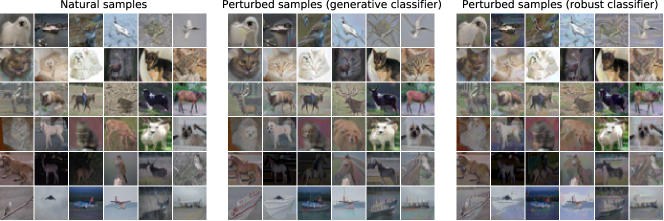
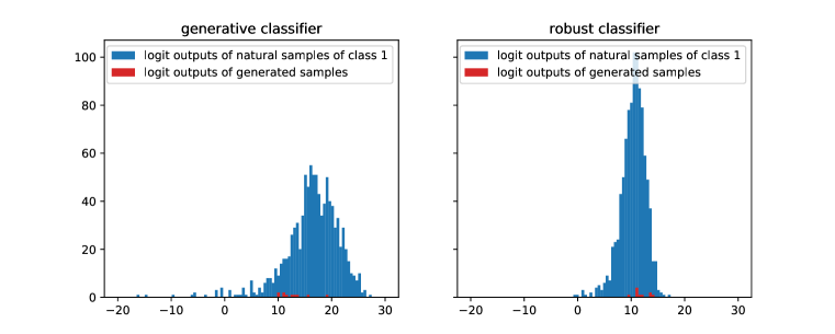
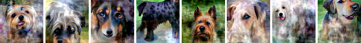
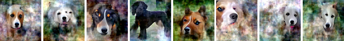
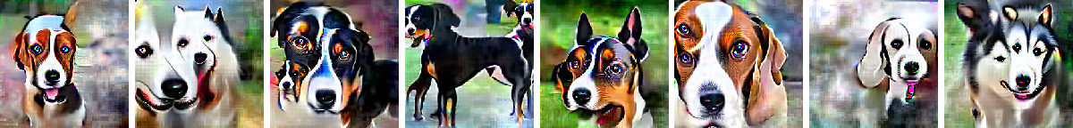
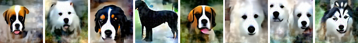
Figure 4 shows perturbed samples produced by performing targeted attacks against the generative classifier and softmax robust classifier. The generative classifier’s perturbation samples have distinguishable visible features of the target class, indicating that individual binary classifiers have learned the class conditional distributions, and the perturbations have to change the semantics for a successful attack. In contrast, perturbations introduced by attacking the softmax robust classifier are not interpretable, even though they can cause high logit output of the target classes (see Figure 9 for the logit outputs distribution).
5.2 CIFAR10
On CIFAR10 we train a single detection model that consists of ten binary classifiers using constrain PGD attack of steps 40 and step size 0.5 (note that the scale of and step size here is 0-255, as opposed to 0-1 as in the case of MNIST). The softmax robust classifier (Madry et al., 2017) that we compare with is also trained with constraint but with a different step size (Appendix C.2.2 provides a discussion on the effects of step size). Appendix A.2 provides the training details.
Robustness results Table 3 shows that and can withstand PGD attacks configured with different steps and step-size. In Appendix C.2.1 we report random restart test results, cross-norm and cross-perturbation test results, and robustness test result for based models.
| PGD attack steps, step-size | ||
|---|---|---|
| 20, 2.0 | 0.9224 | 0.9533 |
| 40, 0.5 | 0.9234 | 0.9553 |
| 200, 0.1 | 0.9231 | 0.9550 |
| 200, 0.5 | 0.9205 | 0.9504 |
| 500, 0.5 | 0.9203 | 0.9500 |
Detection results Consistent with the MNIST result, Fig. 5 shows that combined attack with Eq. 17 is the most effective attack against integrated detection, and generative detection similarly outperforms integrated detection. Table 4 shows that generative detection outperforms the state-of-the-art adversarial detection method.
| Detection method | Mean distortion (0-1 scale) |
|---|---|
| State-of-the-art (Carlini & Wagner, 2017a) | 1.1 |
| Ours (generative detection) | 1.5 |
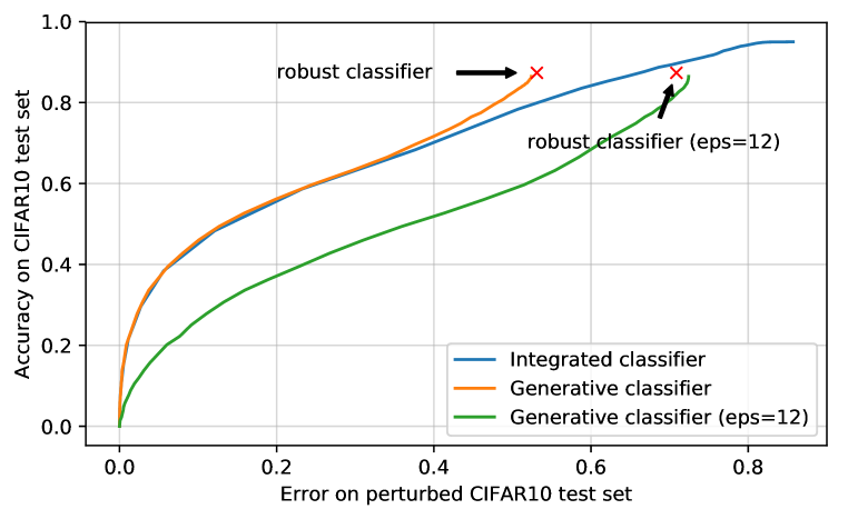
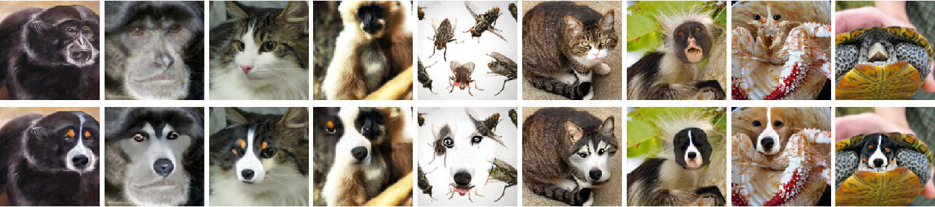
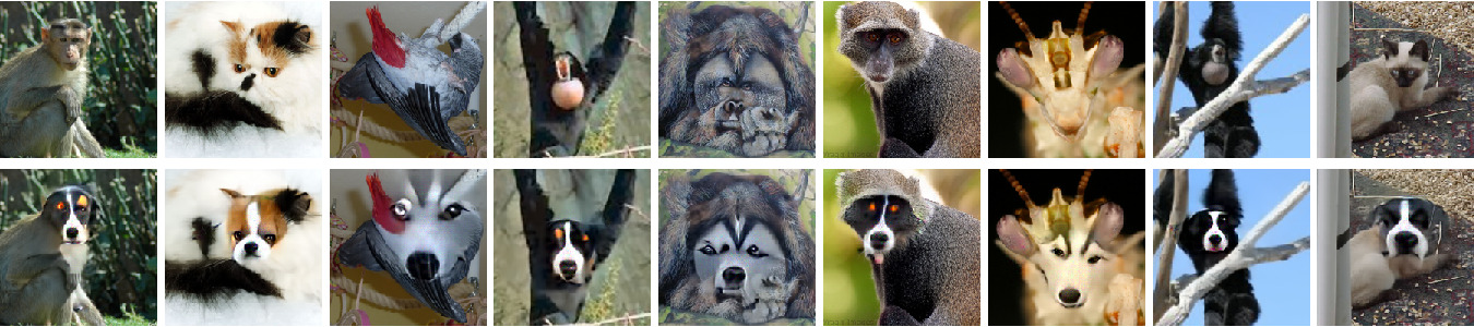
Classification results Contrary to MNIST’s result, we did not observe a dramatic decrease in the softmax robust classifier’s performance when we increase the perturbation limit to (Fig. 5(b)). Integrated classification can reach the standard accuracy of a regular classifier, but at the cost of significantly increased error on the perturbed set. Fig. 6 shows some perturbed samples produced by attacking the generative classifier and robust classifier. While these two classifiers have similar errors on the perturbed set, samples produced by attacking the generative classifier have more visible features of the attacked classes, suggesting that the adversary needs to change more semantic to cause the same error.
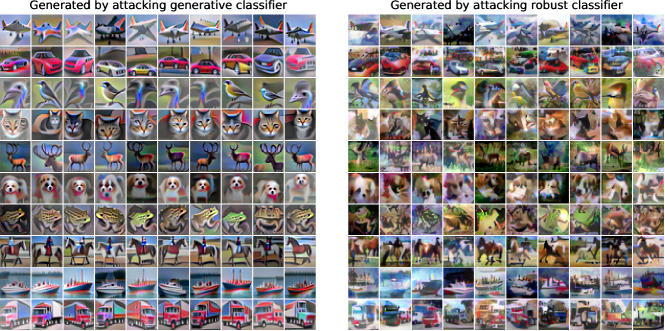
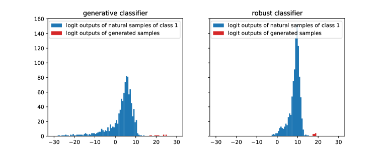
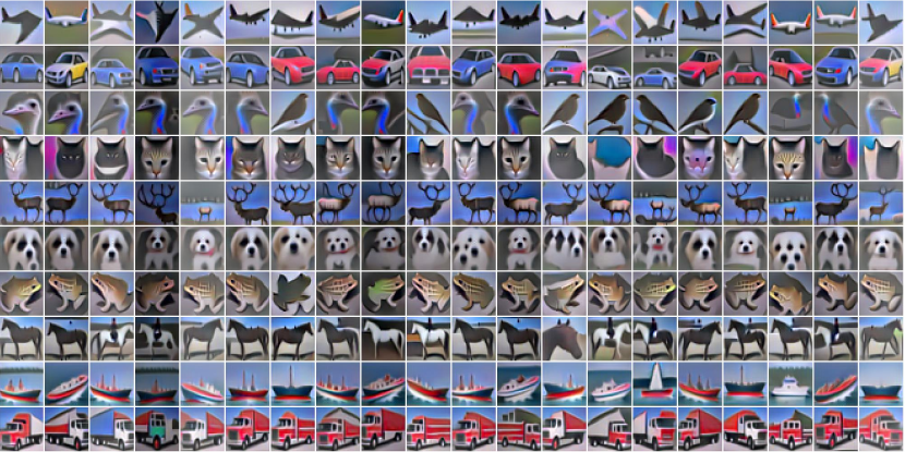
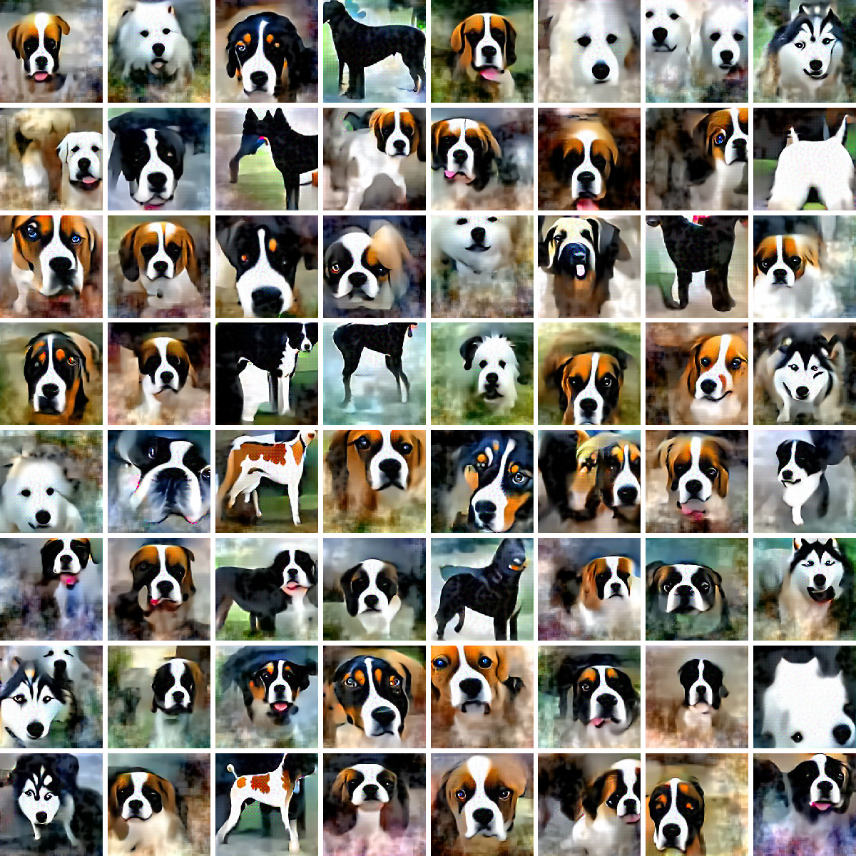
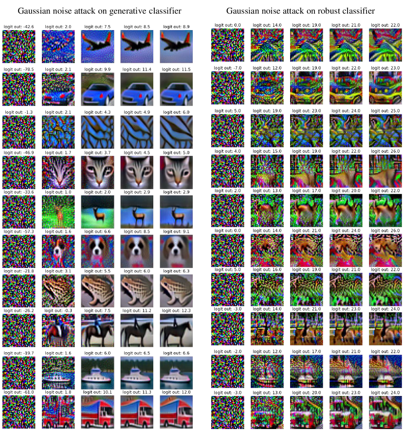
Fig. 7 and Fig. 11 demonstrate that unrecognizable images are able to cause high logit outputs of the softmax robust classifier. This phenomenon highlights a major defect of the softmax robust classifier: they can be easily fooled by unrecognizable inputs (Nguyen et al., 2015; Goodfellow et al., 2014; Schott et al., 2018). In contrast, samples that cause high logit outputs of the generative classifier all have clear semantic meaning. In Figure 14 we present image synthesis results using constrained detectors. In Appendix D we provide Gaussian noise attack results and a discussion about the interpretability of the generative classification approach.
6 Conclusion
We studied the problem of adversarial example detection under the robust optimization framework and proposed a novel detection method that can withstand adaptive attacks. Our formulation leads to a new generative modeling technique which we called generative adversarial training (GAT). GAT’s capability to learn class conditional distributions further gives rise to generative detection/classification approaches that show competitive performance and improved interpretability.
References
- Amodei et al. (2016) Dario Amodei, Sundaram Ananthanarayanan, Rishita Anubhai, Jingliang Bai, Eric Battenberg, Carl Case, Jared Casper, Bryan Catanzaro, Qiang Cheng, Guoliang Chen, et al. Deep speech 2: End-to-end speech recognition in english and mandarin. In International conference on machine learning, pp. 173–182, 2016.
- Athalye et al. (2018) Anish Athalye, Nicholas Carlini, and David Wagner. Obfuscated gradients give a false sense of security: Circumventing defenses to adversarial examples. arXiv preprint arXiv:1802.00420, 2018. URL https://arxiv.org/abs/1802.00420.
- Bahat et al. (2019) Yuval Bahat, Michal Irani, and Gregory Shakhnarovich. Natural and adversarial error detection using invariance to image transformations. arXiv preprint arXiv:1902.00236, 2019.
- Bastani et al. (2016) Osbert Bastani, Yani Ioannou, Leonidas Lampropoulos, Dimitrios Vytiniotis, Aditya Nori, and Antonio Criminisi. Measuring neural net robustness with constraints. In Advances in neural information processing systems, pp. 2613–2621, 2016.
- Bhagoji et al. (2017) Arjun Nitin Bhagoji, Daniel Cullina, and Prateek Mittal. Dimensionality reduction as a defense against evasion attacks on machine learning classifiers. arXiv preprint arXiv:1704.02654, 2017.
- Carlini & Wagner (2017a) Nicholas Carlini and David Wagner. Adversarial examples are not easily detected: Bypassing ten detection methods. In Proceedings of the 10th ACM Workshop on Artificial Intelligence and Security, pp. 3–14. ACM, 2017a. URL https://arxiv.org/abs/1705.07263.
- Carlini & Wagner (2017b) Nicholas Carlini and David Wagner. Towards evaluating the robustness of neural networks. In 2017 IEEE Symposium on Security and Privacy (SP), pp. 39–57. IEEE, 2017b.
- Chen et al. (2018) Pin-Yu Chen, Yash Sharma, Huan Zhang, Jinfeng Yi, and Cho-Jui Hsieh. Ead: elastic-net attacks to deep neural networks via adversarial examples. In Thirty-second AAAI conference on artificial intelligence, 2018.
- Engstrom et al. (2019) Logan Engstrom, Andrew Ilyas, Shibani Santurkar, Dimitris Tsipras, Brandon Tran, and Aleksander Madry. Adversarial robustness as a prior for learned representations. arXiv preprint arXiv:1906.00945, 2019.
- Feinman et al. (2017) Reuben Feinman, Ryan R Curtin, Saurabh Shintre, and Andrew B Gardner. Detecting adversarial samples from artifacts. arXiv preprint arXiv:1703.00410, 2017. URL https://arxiv.org/abs/1703.00410.
- Gong et al. (2017) Zhitao Gong, Wenlu Wang, and Wei-Shinn Ku. Adversarial and clean data are not twins. arXiv preprint arXiv:1704.04960, 2017. URL https://arxiv.org/abs/1704.04960.
- Goodfellow et al. (2014) Ian J Goodfellow, Jonathon Shlens, and Christian Szegedy. Explaining and harnessing adversarial examples. arXiv preprint arXiv:1412.6572, 2014. URL https://arxiv.org/abs/1412.6572.
- Grosse et al. (2017) Kathrin Grosse, Praveen Manoharan, Nicolas Papernot, Michael Backes, and Patrick McDaniel. On the (statistical) detection of adversarial examples. CoRR, 2017.
- Gu & Rigazio (2014) Shixiang Gu and Luca Rigazio. Towards deep neural network architectures robust to adversarial examples. arXiv preprint arXiv:1412.5068, 2014.
- He et al. (2016) Kaiming He, Xiangyu Zhang, Shaoqing Ren, and Jian Sun. Deep residual learning for image recognition. In Proceedings of the IEEE conference on computer vision and pattern recognition, pp. 770–778, 2016.
- He et al. (2018) Warren He, Bo Li, and Dawn Song. Decision boundary analysis of adversarial examples. In International Conference on Learning Representations, 2018. URL https://openreview.net/forum?id=BkpiPMbA-.
- Hendrycks & Gimpel (2017) Dan Hendrycks and Kevin Gimpel. Early methods for detecting adversarial images. In ICLR, 2017. URL https://arxiv.org/abs/1608.00530.
- Jin et al. (2015) Jonghoon Jin, Aysegul Dundar, and Eugenio Culurciello. Robust convolutional neural networks under adversarial noise. arXiv preprint arXiv:1511.06306, 2015.
- Kurakin et al. (2016a) Alexey Kurakin, Ian Goodfellow, and Samy Bengio. Adversarial examples in the physical world. arXiv preprint arXiv:1607.02533, 2016a. URL https://arxiv.org/abs/1607.02533.
- Kurakin et al. (2016b) Alexey Kurakin, Ian Goodfellow, and Samy Bengio. Adversarial machine learning at scale. arXiv preprint arXiv:1611.01236, 2016b.
- LeCun et al. (2006) Yann LeCun, Sumit Chopra, Raia Hadsell, M Ranzato, and F Huang. A tutorial on energy-based learning. Predicting structured data, 1(0), 2006.
- Levine et al. (2016) S Levine, C Finn, T Darrell, and P Abbeel. End-to-end training of deep visuomotor policies. Journal of Machine Learning Research, 17:1334–1373, 2016.
- Li & Li (2017) Xin Li and Fuxin Li. Adversarial examples detection in deep networks with convolutional filter statistics. 2017 IEEE International Conference on Computer Vision (ICCV), pp. 5775–5783, 2017. URL https://arxiv.org/abs/1612.07767.
- Liu et al. (2017) Yuntao Liu, Yang Xie, and Ankur Srivastava. Neural trojans. In 2017 IEEE International Conference on Computer Design (ICCD), pp. 45–48. IEEE, 2017.
- Ma et al. (2018) Xingjun Ma, Bo Li, Yisen Wang, Sarah M Erfani, Sudanthi Wijewickrema, Grant Schoenebeck, Dawn Song, Michael E Houle, and James Bailey. Characterizing adversarial subspaces using local intrinsic dimensionality. arXiv preprint arXiv:1801.02613, 2018. URL https://arxiv.org/abs/1801.02613.
- Madry et al. (2017) Aleksander Madry, Aleksandar Makelov, Ludwig Schmidt, Dimitris Tsipras, and Adrian Vladu. Towards deep learning models resistant to adversarial attacks. arXiv preprint arXiv:1706.06083, 2017. URL https://arxiv.org/abs/1706.06083.
- MadryLab (a) MadryLab. CIFAR10 Adversarial Examples Challenge. https://github.com/MadryLab/cifar10_challenge, a.
- MadryLab (b) MadryLab. MNIST Adversarial Examples Challenge. https://github.com/MadryLab/mnist_challenge, b.
- Metzen et al. (2017) Jan Hendrik Metzen, Tim Genewein, Volker Fischer, and Bastian Bischoff. On detecting adversarial perturbations. CoRR, abs/1702.04267, 2017. URL https://arxiv.org/abs/1702.04267.
- Moosavi-Dezfooli et al. (2016) Seyed-Mohsen Moosavi-Dezfooli, Alhussein Fawzi, and Pascal Frossard. Deepfool: a simple and accurate method to fool deep neural networks. In Proceedings of the IEEE conference on computer vision and pattern recognition, pp. 2574–2582, 2016.
- Nguyen et al. (2015) Anh Nguyen, Jason Yosinski, and Jeff Clune. Deep neural networks are easily fooled: High confidence predictions for unrecognizable images. In Proceedings of the IEEE conference on computer vision and pattern recognition, pp. 427–436, 2015.
- Pang et al. (2018) Tianyu Pang, Chao Du, Yinpeng Dong, and Jun Zhu. Towards robust detection of adversarial examples. In Advances in Neural Information Processing Systems, pp. 4579–4589, 2018. URL https://arxiv.org/abs/1706.00633.
- Papernot et al. (2016a) Nicolas Papernot, Patrick McDaniel, Somesh Jha, Matt Fredrikson, Z Berkay Celik, and Ananthram Swami. The limitations of deep learning in adversarial settings. In 2016 IEEE European Symposium on Security and Privacy (EuroS&P), pp. 372–387. IEEE, 2016a.
- Papernot et al. (2016b) Nicolas Papernot, Patrick McDaniel, Xi Wu, Somesh Jha, and Ananthram Swami. Distillation as a defense to adversarial perturbations against deep neural networks. In 2016 IEEE Symposium on Security and Privacy (SP), pp. 582–597. IEEE, 2016b.
- Roth et al. (2019) Kevin Roth, Yannic Kilcher, and Thomas Hofmann. The odds are odd: A statistical test for detecting adversarial examples. arXiv preprint arXiv:1902.04818, 2019.
- Santurkar et al. (2019) Shibani Santurkar, Dimitris Tsipras, Brandon Tran, Andrew Ilyas, Logan Engstrom, and Aleksander Madry. Image synthesis with a single (robust) classifier, 2019.
- Schott et al. (2018) Lukas Schott, Jonas Rauber, Matthias Bethge, and Wieland Brendel. Towards the first adversarially robust neural network model on mnist. arXiv preprint arXiv:1805.09190, 2018.
- Shafahi et al. (2018) Ali Shafahi, W Ronny Huang, Mahyar Najibi, Octavian Suciu, Christoph Studer, Tudor Dumitras, and Tom Goldstein. Poison frogs! targeted clean-label poisoning attacks on neural networks. In Advances in Neural Information Processing Systems, pp. 6103–6113, 2018.
- Shen et al. (2017) Dinggang Shen, Guorong Wu, and Heung-Il Suk. Deep learning in medical image analysis. Annual review of biomedical engineering, 19:221–248, 2017.
- Sinha et al. (2018) Aman Sinha, Hongseok Namkoong, and John Duchi. Certifiable distributional robustness with principled adversarial training. In International Conference on Learning Representations, 2018. URL https://openreview.net/forum?id=Hk6kPgZA-.
- Su et al. (2019) Jiawei Su, Danilo Vasconcellos Vargas, and Kouichi Sakurai. One pixel attack for fooling deep neural networks. IEEE Transactions on Evolutionary Computation, 2019.
- Szegedy et al. (2013) Christian Szegedy, Wojciech Zaremba, Ilya Sutskever, Joan Bruna, Dumitru Erhan, Ian Goodfellow, and Rob Fergus. Intriguing properties of neural networks. arXiv preprint arXiv:1312.6199, 2013. URL https://arxiv.org/abs/1312.6199.
- Tian et al. (2018) Shixin Tian, Guolei Yang, and Ying Cai. Detecting adversarial examples through image transformation. In Thirty-Second AAAI Conference on Artificial Intelligence, 2018.
- Tramer et al. (2020) Florian Tramer, Nicholas Carlini, Wieland Brendel, and Aleksander Madry. On adaptive attacks to adversarial example defenses. arXiv preprint arXiv:2002.08347, 2020.
- Tsipras et al. (2018) Dimitris Tsipras, Shibani Santurkar, Logan Engstrom, Alexander Turner, and Aleksander Madry. Robustness may be at odds with accuracy. stat, 1050:11, 2018. URL https://arxiv.org/abs/1805.12152.
- Vaswani et al. (2017) Ashish Vaswani, Noam Shazeer, Niki Parmar, Jakob Uszkoreit, Llion Jones, Aidan N Gomez, Łukasz Kaiser, and Illia Polosukhin. Attention is all you need. In Advances in neural information processing systems, pp. 5998–6008, 2017.
- Xiao et al. (2018) Chaowei Xiao, Bo Li, Jun-Yan Zhu, Warren He, Mingyan Liu, and Dawn Song. Generating adversarial examples with adversarial networks. In Proceedings of the 27th International Joint Conference on Artificial Intelligence, pp. 3905–3911. AAAI Press, 2018.
- Xu et al. (2017) Weilin Xu, David Evans, and Yanjun Qi. Feature squeezing: Detecting adversarial examples in deep neural networks. arXiv preprint arXiv:1704.01155, 2017.
- Zheng & Hong (2018) Zhihao Zheng and Pengyu Hong. Robust detection of adversarial attacks by modeling the intrinsic properties of deep neural networks. In Advances in Neural Information Processing Systems, pp. 7913–7922, 2018.
Appendix A Training Details
A.1 MNIST training
We use 50K samples from the original training set for training and the remaining 10K samples for validation, and report the test performance based on the checkpoint which has the best validation performance. All binary classifiers are trained for 100 epochs, where in each iteration we sample 32 in-class samples as the positive samples, and 32 out-class samples to create adversarial examples which will be used as negative samples.
All binary classifier models use a neural network consisting of two convolutional layers each with 32 and 64 filters, and a fully connected layer of size 1024; more details of the network architecture can be found in Madry et al. (2017).
| models | models | ||||
|---|---|---|---|---|---|
| PGD attack steps, step-size (training) | 100, 0.1 | 200, 0.1 | 100, 0.01 | 100, 0.01 | |
| PGD attack steps, step-size (validation) | 200, 0.1 | 200, 0.1 | 200, 0.01 | 200, 0.01 | |
A.2 CIFAR10 training
We train CIFAR10 binary classifiers using a ResNet model (same as the one used by Madry et al. (2017); MadryLab (a)). To speedup training, we take advantage of a clean trained classifier: the subnetwork of that defines the output logit is essentially a “binary classifier” that would output high values for samples of class , and low values for others. The binary classifier is then trained by finetuning the subnetwork using objective 5. The pretrained classifier has a test accuracy of 95.01% (fetched from MadryLab (a)).
At each iteration of training we sample a batch of 300 samples, from which in-class samples are used as positive samples, while an equal number of out-of-class samples are used for crafting adversarial examples. Adversarial examples for training and models are both optimized using normalized steepest descent based PGD attacks (MadryLab, b). We report results based on the best performances on the CIFAR10 test set (thus don’t claim generalization performance of the proposed method).
Appendix B Computing mean distance
We first find the detection threshold with which the detection system has 0.95 TPR. We construct a new loss function by adding a weighted loss term that measures perturbation size to objective 14
| (21) |
We then use unconstrained PGD attack to optimize . We use binary search to find the optimal , where in each bsearch attempt if is a false positive ( and ) we consider the current as effective and continue with a larger . The configurations for performing binary search and PGD attack are detailed in Table 6. The upper bound is established such that with this upper bound, no samples except those that are inherently misclassified by the generative classifier, could be perturbed as a false positive. With these settings, our MNIST and generative detection models respective reached 1.0 FPR and 0.9455 FPR, and CIFAR10 generative model reached 0.9995 FPR.
| Dataset | Initial | lower bound | upper bound | bsearch depth | PGD steps | PGD step size | Threshold | PGD optimizer |
|---|---|---|---|---|---|---|---|---|
| MNIST | 0.0 | 0.0 | 8.0 | 20 | 1000 | 1.0 (0-1 scale) | 3.6 | Adam |
| CIFAR10 | 0.0 | 0.0 | 1.0 | 20 | 100 | 2.56 (0-255 scale) | -5.0 | normalized steepest descent |
Appendix C More experimental results
C.1 More MNIST results
| PGD attack steps, step size | model | model | ||
|---|---|---|---|---|
| 200, 0.01 | 0.99962 | 0.99973 | 0.99820 | 0.99901 |
| 2000, 0.005 | 0.99959 | 0.99971 | 0.99795 | 0.99872 |
| PGD attack steps, step size | model | model | ||
|---|---|---|---|---|
| 200, 0.1 | 0.99906 | 0.99916 | 0.99960 | 0.99997 |
| 2000, 0.05 | 0.99855 | 0.99883 | 0.99237 | 0.99994 |
| Attack | |||||||||
|---|---|---|---|---|---|---|---|---|---|
| 0.99959 | 0.99966 | 0.99927 | 0.99925 | 0.99971 | 0.99967 | 0.99949 | 0.99984 | ||
| 0.99436 | 0.9983 | 0.99339 | 0.99767 | 0.99778 | 0.99869 | 0.99397 | 0.99961 | ||
| 0.99974 | 0.99969 | 0.99962 | 0.99944 | 0.99965 | 0.99955 | 0.99968 | 0.99987 | ||
| 0.96421 | 0.98816 | 0.97747 | 0.99577 | 0.98268 | 0.98687 | 0.98117 | 0.99986 | ||
| model | model | |
|---|---|---|
| fixed start | 0.99830 | 0.99578 |
| 50 random restarts | 0.99776 | 0.99501 |
| AUC | 0.99959 | 0.99971 | 0.99876 | 0.99861 | 0.99859 | 0.99861 | 0.99795 | 0.99863 | 0.99687 | 0.99418 |
| AUC | 0.99830 | 0.99869 | 0.99327 | 0.99355 | 0.99314 | 0.99228 | 0.99424 | 0.99439 | 0.97875 | 0.9769 |
C.2 More CIFAR10 results
C.2.1 More robustness test results
| model | model | |
|---|---|---|
| fixed start | 0.9866 | 0.9234 |
| 10 random starts | 0.9866 | 0.9233 |
| PGD attack | AUC |
|---|---|
| -constrained (steps 20, step-size 10) | 0.9814 |
| -constrained (steps 10, step-size 0.5) | 0.9841 |
| -constrained PGD attack steps, step size | ||
|---|---|---|
| 20, 10 | 0.9839 | 0.9924 |
| 50, 5.0 | 0.9837 | 0.9922 |
| AUC | 0.9866 | 0.9926 | 0.9721 | 0.9501 | 0.9773 | 0.9636 | 0.9859 | 0.9908 | 0.9930 | 0.9916 |
| AUC | 0.9234 | 0.9553 | 0.8393 | 0.7893 | 0.8494 | 0.8557 | 0.9071 | 0.9276 | 0.9548 | 0.9370 |
C.2.2 Training step size and robustness
We found training with adversarial examples optimized with a sufficiently small step size to be critical for model robustness. In table 17 we tested two binary classifiers respectively trained with 0.5 and 1.0 step size. The step size 1.0 model is not robust when tested with a much smaller step size. We observe that when training the step size 1.0 model, training set adv AUC reached 1.0 in less than one hundred iterations, but test set clean AUC plummeted to around 0.95 and couldn’t recover thereafter. (Please refer to Figure 12 for the definitions of adv AUC and nat AUC.)
| Attack steps, step-size | Training steps, step-size | |
|---|---|---|
| 10, 0.5 | 10, 1.0 | |
| 10, 0.5 | 0.9866 | 0.9965 |
| 40, 0.1 | 0.9892 | 0.8848 |
C.2.3 Effects of perturbation limit
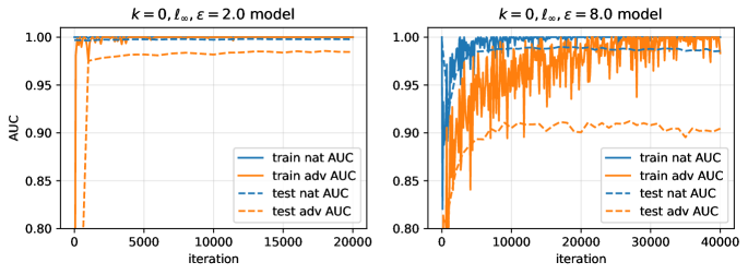
To study the effects of perturbation limit, we analyze the training dynamics of one constrained and one constrained binary classifiers. In Figure 12 we show the training and testing history of these two models. The model history shows that by adversarial finetuning the model reaches robustness in just a few thousands of iterations, and the performance on clean samples is preserved (test clean AUC begins at 0.9971, and ends at 0.9981). Adversarial finetuning on the model didn’t converge after an extended 20K iterations of training. The gap between train adv AUC and test adv AUC of the model is more pronounced, and we observed a decrease of test clean AUC from 0.9971 to 0.9909.
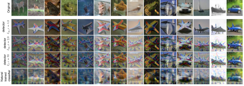
These results suggest that training with larger perturbation limit is more time and resource consuming, and could lead to performance decrease on clean samples. The benefit is that the detector is pushed to a better approximation of the target data distribution. As an illustration, in Figure 13, perturbations generated by attacking the naturally trained classifier (corresponds to 0 perturbation limit) don’t have clear semantics, while perturbed samples of the model are completely recognizable.
C.3 ImageNet results
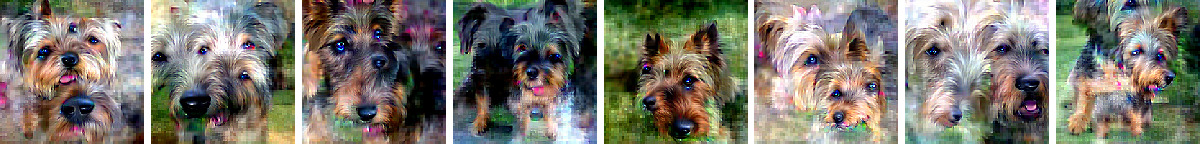
On ImageNet we show GAT induces detection robustness and supports the learning of class conditional distributions. Our experiment is based on Restricted ImageNet (Tsipras et al., 2018), a subset of ImageNet that has its samples reorganized into customized categories. The dog category consists of images of different breeds collected from ImageNet class from 151 to 268. We trained a dog class detector by finetuning a pre-trained ResNet50 (He et al., 2016) model. The dog category covers a range of ImageNet classes, with each one having its logit output. We use the subnetwork defined by the logit output of class 151 as the detector (in principle logit output of other classes in the range should also work). Due to computational resource constraints, we only validated the robustness of a trained detector (trained with PGD attack of steps 40 and step size 0.001), and we present the result in Table 18. (On Restricted ImageNet in the case of scenario Tsipras et al. (2018) only demonstrates the robustness of a constrained model). Please refer to Appendix C.3 for more results on adversarial example generation and image synthesis.
| Attack steps, step size | 40, 0.001 | 100, 0.001 | 200, 0.001 | 40, 0.002 | 200, 0.002 | 200, 0.0005 |
| AUC | 0.9720 | 0.9698 | 0.9692 | 0.9703 | 0.9690 | 0.9698 |

Appendix D Gaussian noise attack and model interpretability
In this section we use Gaussian noise attack experiment to motivate a comparative analysis of the interpretabilities of our generative classification approach and discriminative robust classification approach (Madry et al., 2017).
We first discuss how these two approaches determine the posterior class probabilities.
For the discriminative classifier, the posterior probabilities are computed from the logit outputs of the classifier using the softmax function . For the generative classifier, the posterior probabilities are computed in two steps: in the first, we train the base detectors, which is the process of solving the inference problem of determining the joint probability , and in the second, we use Bayes rule to compute the posterior probability . Coincidentally, the formulas for computing the posterior probabilities take the same form. But in our approach, the exponential of the logit output of a detector (i.e., ) has a clear probabilistic interpretation: it’s the unnormalized joint probability of the input and the corresponding class category. We use Gaussian noise attack to demonstrate that this probabilistic interpretation is consistent with visual perception.
We start from a Gaussian noise image, and gradually perturb it to cause higher and higher logit outputs. This is implemented by targeted PGD attack against logit outputs of these two classification models. The resulting images in Figure 19 show that, in our model, the logit output increase direction, i.e. the join probability increase direction, indicates the class semantic changing direction; while for the discriminative robust model, the perturbed image computed by increasing logit outputs are not as clearly interpretable. In particular, the perturbed images that cause high logit outputs of the softmax robust classifiers are not recognizable.
In summary, as a generative classification approach that explicitly models class conditional distributions, our system offers a probabilistic view of the decision making process of the classification problem; adversarial attacks that rely on imperceptible or uninterpretable noises are not effective against such a system.
Appendix E Computational cost issue
In this section we provide an analysis of the computational cost of our generative classification approach. In terms of memory requirements, if we assume the softmax classifier (i.e., the discriminative softmax robust classifier) and the detectors use the same architecture (i.e., only defer in the final layer) then the detector based generative classifier is approximately times more expensive than the -class softmax classifier. This also means that the computational graph of the generative classifier is times larger than the softmax classifier. Indeed, in the CIFAR10 task, on our Quadro M6000 24GB GPU (TensorFlow 1.13.1), the inference speed of the generative classifier is roughly ten times slower than the softmax classifier.
We next benchmark the training speed of these two types of classifiers.
The generative classifier has logit outputs, with each one defined by the logit output of a detector. Same with the softmax classifier, except that the outputs share the parameters in the convolutional base. Now consider ordinary adversarial training on the softmax classifier and generative adversarial training on the generative classifier. To train the softmax classifier, we use batches of samples. For the generative classifier, we train each detector with batches of samples ( positive samples and negative samples). At each iteration, we need to respectively compute and adversarial examples for these two classifiers. Now we test the speed of the following two scenarios: 1) compute the gradient w.r.t. to N samples on a single computational graph, and 2) compute the gradient w.r.t to samples on computational graphs, with each graph working on samples. We assume that in scenario 2 all the computational graphs are loaded to GPUs, and thus their computations are in parallel.
In our CIFAR10 experiment, we used batches consisting of 30 positive samples and 30 negative samples to train each ResNet50 binary classifiers. In Madry et al. (2017), the softmax classifier was trained with batches of 128 samples. In this case, , , and . On our GPU, scenario 1 took 683 ms 6.76 ms per loop, while scenario 2 took 1.85 s 42.7 ms per loop. In this case, we could expect generative adversarial training to be about 2.7 times slower than ordinary adversarial training, if not considering parameter gradient computation.
In practice, large batch size is almost always preferred. And our method won’t compare as favorably if we choose to use one.
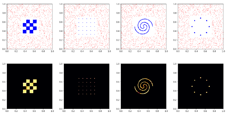
Appendix F Density estimation on synthetic datasets
While ordinary discriminative training only learns a good decision boundary, GAT is able to learn the underlying density functions that generate the training data. Results on 1D (Figure 20) and 2D benchmark datasets (Figure 21) show that through properly configured generative adversarial training, detectors’ output recover target density functions.