Infusing domain knowledge in AI-based ”black box” models for better explainability with application in bankruptcy prediction

Abstract.

Although ”black box” models such as Artificial Neural Networks, Support Vector Machines, and Ensemble Approaches continue to show superior performance in many disciplines, their adoption in the sensitive disciplines (e.g., finance, healthcare) is questionable due to the lack of interpretability and explainability of the model. In fact, future adoption of ”black box” models is difficult because of the recent rule of ”right of explanation” by the European Union where a user can ask for an explanation behind an algorithmic decision, and the newly proposed bill by the US government, the ”Algorithmic Accountability Act”, which would require companies to assess their machine learning systems for bias and discrimination and take corrective measures. Top Bankruptcy Prediction Models are A.I.-Based and are in need of better explainability–the extent to which the internal working mechanisms of an AI system can be explained in human terms. Although explainable artificial intelligence is an emerging field of research, infusing domain knowledge for better explainability might be a possible solution. In this work, we demonstrate a way to collect and infuse domain knowledge into a ”black box” model for bankruptcy prediction. Our understanding from the experiments reveals that infused domain knowledge makes the output from the black box model more interpretable and explainable.

1. Introduction

Over the past few years, the field of Artificial Intelligence (AI) has gained enormous interest for its practical success in many application areas. Recent advances in machine learning and artificial intelligence have given rise to many complex and powerful models which are being adopted in many sophisticated areas such as medical, finance, and cyber-security. Some of the more notable models are Artificial Neural Networks (ANN), Genetic Algorithms (GA), Support Vector Machines (SVM), and Ensemble Approaches. Sometimes these models are called ”black box” models. Although the high complexity of the models’ non-linear functions come with good predictive power for black box models, they are limited by their explanation and interpretation capabilities. Which is followed by a lack of trust in the model and the decisions it makes.

In response to that issue, as a precaution to fight the unethical use of AI and biases in decision making, governments are trying to introduce and enforce new laws and regulations. For instance, the European Union implemented the rule of ”right of explanation”, where a user can ask for an explanation of an algorithmic decision (Goodman and Flaxman, 2017). In addition, more recently, the US government has introduced a new bill called the ”Algorithmic Accountability Act” (alg, [n. d.]) which would require companies to assess their machine learning systems for bias and discrimination and take corrective measures. Should the bill pass, it will be enforced by the US Federal Trade Commission which is in charge of consumer protection and antitrust regulation.

Black box models are frequently used in the financial area, particularly towards bankruptcy prediction. In particular, the main focus of bankruptcy prediction is to predict the probability that the customer will be in default or bankrupt in the near future. The high rate of bankruptcy affects heavily the firm’s owners, partners, society, and the overall economic condition of the country in general (Alaka et al., 2018). According to literature reviews by Alaka et al. (Alaka et al., 2018) and Bellovary et al. (Bellovary et al., 2007), six out of the top eight Bankruptcy Prediction Model (BPM) are Artificial Intelligence (AI) based. They also suggest that BPMs based on ”black box” models such as ANN, GA, and SVM outperform all other models due to their capability of learning any non-linear function. Recently another black box model, ensemble approaches, where multiple models are combined for better results by correcting each other’s error, shows promising performances. However, these ”black box” models lack explainability (i.e., explaining the internal working mechanism to humans) and interpretability (i.e., a sense of what’s happening), which raises ethical issues for domains like finance. A decision in the financial domain (e.g., credit approval, default prediction) needs to be more than a number— it needs to explain the reason behind the decision that makes sense to a human. Furthermore, when there are many explanatory variables, and some explanatory variables are complex, this further complicates the explainability.

Research in Explainable Artificial Intelligence is an emerging field, seeing a resurgence after three decades of slowed progress since the work of Chandrasekaran et al. (Chandrasekaran et al., 1989), Swartout et al. (Swartout and Moore, 1993), and Buchanan et al. (Swartout, 1985). In their work on Explainable Artificial Intelligence(XAI), Miller et al. (Miller, 2018) argue that most of the work on XAI focuses on the researcher’s intuition of what constitutes a good explanation. However, there exists a vast area of research in philosophy, psychology, and cognitive science on how people generate, select, evaluate, and represent explanations and associated cognitive biases and social expectations towards the explanation process. Therefore, the author emphasizes that, the research on explainable AI should incorporate study from these different domains.

According to Lipton et al. (Lipton, 2016) and (on_, [n. d.]c), interpretability has three different notions:

1. interpretability in pre-modeling: finding and using simple, summarized, and relevant set of features from the domain;

2. interpretability in modeling: generating explanation along with the prediction to improve transparency;and

3. interpretability in post modeling (a.k.a. post-hoc): understanding the dynamics between input and predicted output for an already trained/tested model.

Unfortunately, the post-hoc notion of interpretability is not purely transparent and can be misleading, as it provides an explanation after the decision has been made. The algorithm can be optimized to placate subjective demand, and the explanation from it also can be misleading though it seems plausible (Lipton et al. 2016) (Lipton, 2016), (on_, [n. d.]c). Furthermore, from the literature review, we find that interpretability in pre-modeling is under-focused. Therefore, we particularly focus on the explainability of black box models using domain knowledge which falls into interpretability in the pre-modeling stage. In this work, we take bankruptcy prediction as the context for our experiments.

In our proposed approach, we replace hard to interpret features of a model with easily interpretable features (induced from domain knowledge) which allows the decision to be expressed in terms of an interpretable and concise set of features. We use a frequent pattern mining algorithm to find frequent feature sets used in different bankruptcy literature. Later, we relate the frequent feature set with the popular financial concept of credit to come up with a generalized feature set for the experiments, which ultimately allows us to infuse domain knowledge to increase the explainability and interpretability of ”black box” models. To asses credit risk by human experts, the 5C’s of credit is commonly used to analyze key factors: character (reputation of the borrower/firm), capital (leverage), capacity (volatility of the borrower’s earnings), collateral (pledged asset) and cycle (macroeconomic) conditions (Angelini et al., 2008; 5cs, [n. d.]). The domain knowledge infused feature set gives us a generalized frequent feature set which is used for our experiments for better explainability.

In summary, our contributions in this work are as follows: (1) we demonstrate a way to collect and use domain knowledge from the literature; (2) we introduce a way to bring popular concepts (e.g., the 5 C’s of credit) from literature to aid in interpretability and explainability; and (3) our experimental results show ”black box” models can be better explainable with little or no compromise in performance when domain knowledge is infused.

We start with a background of related work (Section 2) followed by a description of our proposed approach and an overview of the dataset (Section 3) used in this work. In Section 4, we describe our experiments, followed by section 5 which contains results and a discussion of the experiments. We conclude with limitations and future work in section 6.

2. background

Early research in explainable AI started with the preliminary work of Chandrasekaran et al. (Chandrasekaran et al., 1989), Swartout et al. (Swartout and Moore, 1993), and Buchanan et al. (Swartout, 1985). Recent advancements in AI, successful adoption in different applications, and awareness of ethical and bias issues necessitates have fueled recent research in Explainable Artificial Intelligence (XAI). For instance, the DARPA division of the Department of Defense (DoD) is spending $2 billion on its XAI program. They are developing a toolkit library consisting of machine learning and human-computer interface software for developing explainable AI systems that will be available for military and commercial use (exp, [n. d.]).

Yang et al. (Yang and Shafto, 2017), propose a method based on ”Bayesian Teaching”, where a subset of an example in used to train the model instead of the whole dataset. The subset of the example is chosen by domain experts that are most relevant to the problem. However, for this purpose, choosing the right subset of examples in the real world is challenging.

In sentiment analysis, the rationale for a prediction is important for understanding decisions. Lei et al. (Lei et al., 2016) propose an approach that generates the rationale for a prediction. They demonstrate the approach with sentiment analysis from the text where a subset of text is selected as the rationale for the prediction. In addition, the selected text is concise and sufficient enough to act as a substitute for the original text, still capable of the correct prediction. Although their approach outperforms available attention-based models, it is limited to only text analysis.

Making a prediction that can be trusted is another challenge. Ribeiro et al. (Ribeiro et al., 2016) propose a novel explanation technique capable of explaining the prediction of any classifier in an interpretable and faithful manner by learning an interpretable model locally around the prediction. Their concern is on two issues: (1) whether the user should trust the prediction of the model and act on that, and (2) whether the user should trust a model to behave reasonably well when deployed. In addition, they involve human judgment in their experiment to decide whether to trust the model or not.

Lundberg et al. (Lundberg and Lee, 2017) propose a unified approach called ”SHAP” which unifies seven previous approaches: LIME (Ribeiro et al., 2016), DeepLIFT (Shrikumar et al., 2017), Tree Interpreter (Ando, [n. d.]), QII (Datta et al., 2016), Shapley sampling values (Štrumbelj and Kononenko, 2014), Shapley regression values (Lipovetsky and Conklin, 2001), and Layer-wise relevance propagation (Bach et al., 2015) to make the explanation of prediction for any machine learning model. Both LIME (Ribeiro et al., 2016) and SHAP (Lundberg and Lee, 2017) use a simplified input mapping, mapping the original input to a simplified set of input. However, none of the models incorporate domain knowledge. The following approach infuses domain knowledge into the experiment and works as a substitute for original complex features in order to generate a prediction which is explainable by itself.

3. Methodology

The proposed approach consists of two components: a feature generalizer, which gives a generalized frequent feature set with the help of domain knowledge, and an evaluator, that produces and compares the results using the generalized feature set from the original feature set.

3.1. Feature Generalizer

First, the frequent feature miner takes multiple different sets of features used in different bankruptcy prediction literature (see section 3.4) to discover the most frequent set of features (i.e., a frequent combination of features used in different literature) using a popular and classic frequent pattern mining algorithm called Apriori (Agrawal et al. (Agrawal et al., 1994)). In Figure 1, the input to the algorithm is: X₁, X₂,…. X_n $\in$ X where X is the universal set of features used in mortgage bankruptcy prediction literature. The output is some frequent set of features with a specified support and maximum count of features in the set: X_f1, X_f2,…..X_m $\in$ X where X is the universal set of features as before, but here m is much smaller than n. Finally, the frequent set of features is fed into the domain knowledge mapper. In the domain knowledge mapper, a popular, easy to understand and interpret domain concept is introduced and mapped with the frequent feature set. For our case, we introduce the 5Cś of credit which refers to capital, character, cash flow, conditions, and collateral. Based on the mapping, the domain knowledge mapper outputs a generalized frequent feature set infused with domain knowledge.

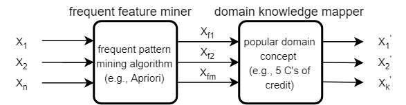
Figure 1. Feature generalizer

3.2. Evaluator

The task of the evaluator (Figure 2) is to execute and compare the performance of two experiments: one using original features (X) of the dataset and the other one using the generalized frequent feature sets (X’). If the difference is within an allowable threshold, then the output from the latter experiment is deemed as final output, and the output is explained using the contribution from each of generalized, and more explainable and interpretable, frequent features.

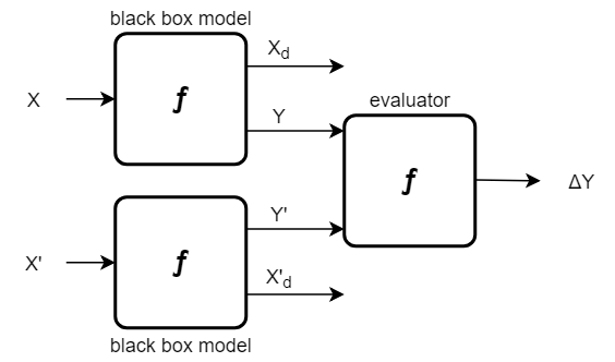
Figure 2. Evaluator

3.3. Algorithms

We use six different algorithms: one is for frequent pattern mining, and the remaining five are supervised ”black box” models for predicting bankruptcy/default.

3.3.1. Apriori

The Apriori algorithm which was proposed by Agrawal et al. (Agrawal et al., 1994), a classical algorithm in data mining for finding frequent patterns. For our case, when a set of features or explanatory variables found in a paper meets a user-specified support threshold, then that set of features can be treated as frequent feature sets. The support for a set of features X in a paper p_i is defined as follows: Support (X) = (number of paper in which all features of X appear) / (total number of paper). For example, if the support threshold is set to .5 (i.e., 50%), then the feature set LTV, creditScore, interestRate, delinquencyStatus is called a frequent feature set if and only if this set of features is found together at least 50% of times among all the papers. Here is an intuition of the working mechanism of the Apriori algorithm. The Apriori algorithm iteratively finds frequent feature sets of a length starting from 1 to k, where k is the maximum number of features in any frequent feature set. The frequent feature sets must meet the minimum support threshold of the algorithm. In addition, a subset of features from the frequent feature set must also be a frequent feature. For example, if LTV, creditScore, interestRate, delinquencyStatus is a frequent feature set, then any of the features or any combination of features (e.g., LTV , LTV, creditScore) within this feature set is also a frequent feature set. In section 4, we will clarify this more.

3.3.2. Artificial Neural Network (ANN)

An Artificial Neural Network is a non-linear model, capable of mimicking human brain functions. It consists of an input layer, multiple hidden layers, and the output layer. Each layer consists of multiple neurons that help to learn the complex pattern, each subsequent layer learns more abstract concepts before it finally merges into the output layer. ANN was first used in 1994 by Wilson and Sharda (Wilson and Sharda, 1994) for bankruptcy prediction. In terms of different performance metrics, given enough data, ANN performs best for many problems due to its capability of learning any non-linear function.

3.3.3. Support Vector Machine (SVM)

The Support Vector Machine (SVM) was first introduced by Boser, Guyon, and Vapnik (Boser et al., 1992) and has been used for many supervised classification tasks. The model learns an optimal hyperplane that separates instances of different classes using a highly non-linear mapping of input vectors in high dimensional feature space [Hooman, 2016]. SVM is listed as one of the top nonlinear algorithms for bankruptcy prediction in different literature surveys (Alaka et al., 2018; Bellovary et al., 2007). When the number of samples is too high (i.e., millions) then it is very costly in terms of computation time. In that case, a non-linear algorithm like ANN can be a better choice as an ANN usually works well with large datasets.

3.3.4. Random Forest (RF)

A Random Forest is a tree-based ensemble technique developed by Breiman et al. (Breiman, 2001) for the supervised classification task. In RF, many trees are generated from the bootstrapped subsamples (i.e., random sample drawn with replacement) of the training data. In each tree, the splitting attribute is chosen from a smaller random subset of attributes of that tree (i.e., the chosen split attribute that is the best among that random subset). This randomness helps to make trees less correlated as correlated trees makes the same kinds of prediction errors and can overfit the model. This results in a forest of trees being generated, and the output from all the trees are averaged for the final prediction. This averaging helps to reduce the variance from the model. Furthermore, RF can work in a parallel computing environment as trees can be grown independently. According to (Fitzpatrick and Mues, 2016), RF has been used in different credit scoring and customer attrition applications.

3.3.5. Extra Trees (ET)

Extremely Randomized Trees or Extra Trees (ET) is also a tree-based ensemble technique like RF and share a similar concept with RF. The only difference is in the process of splitting attribute selection and determining the threshold (cutoff) value, both are chosen in extremely random fashion (Islam et al., 2018b). As in RF, a random subset of features are taken into consideration for the split selection but instead of choosing the most discriminative cut off threshold, ET cut off thresholds are set to random values. Thus, the best of these randomly chosen values is set as the threshold for the splitting rule (ens, [n. d.]). As a result of multiple trees, the variance is reduced, compared to Decision Trees, however bias is introduced, as a subset of the whole feature set is chosen for each tree. The ET which was proposed by Geurts et al.(Geurts et al., 2006), has continued its success by achieving the state of the art performance in some anomaly/intrusion detection research (Islam, 2018; Islam et al., 2018a, b).

3.3.6. Gradient Boosting (GB)

Friedman et al. (Friedman, 2001), generalized Adaboost to a Gradient Boosting algorithm that allows a variety of loss function. Here the shortcoming of weak learners is identified using the gradient, while in AdaBoost it is done through highly weighted data points. Gradient Boosting (GB) is a classifier/regression model in the form of an ensemble of weak prediction models, such as Decision Trees which are fitted with data initially. It also works sequentially like the AdaBoost algorithm, in that each subsequent model tries to minimize the loss function (i.e., Mean Squared Error) by paying special focus on instances that were hard to get right in previous steps.

3.4. Data

We use two sources of data in this work:

1. Explanatory variables dataset: We went through the following 33 research papers related to mortgage bankruptcy prediction: (Bhattacharya et al., 2019; Greenwald, 2018; Kvamme et al., 2018; Kim et al., 2018; Fout et al., 2018; Wu and Dorfman, 2018; Liu and Sing, 2018; Karamon et al., 2017; Sirignano et al., 2016; Sousa et al., 2016; Chan et al., 2016; Fitzpatrick and Mues, 2016; Sirignano and Giesecke, 2018; Hooman et al., 2016; Tian et al., 2016; Moulton et al., 2016; Fang et al., 2016; Antinolfi et al., 2016; Berka, 2016; Bradley et al., 2015; Alfaro and Gallardo, 2012; Khandani et al., 2010; Sousa et al., 2015; SOUSA et al., 2015; Anderson and Jozwik, 2014; Goodman et al., 2014; Foote and Willen, 2018; Ghent and Kudlyak, 2011; Elul et al., 2010; Demiroglu et al., 2014; Low, 2015; Gyourko and Tracy, 2014; Sorenson, 2015) . We collected the explanatory variables used in each of these papers. We made the dataset available to the research community at here (rev, [n. d.]). Table 1 lists the features that appear four or more times in the literature.

2. Freddie Mac single-family loan-level dataset: The Freddie Mac dataset (fre, [n. d.]) is the most frequently used dataset in the 33 previously mentioned research papers. It is also a publicly available dataset. For ensuring transparency, supporting the risk-sharing initiative, and building more accurate credit performance models, Freddie Mac, a government-sponsored enterprise, is making available loan-level credit performance data on fixed-rate mortgages that the company purchased or guaranteed. This is the source of data for the supervised algorithms used in this work. We took a stratified sample of the data to make sure the ratio of default vs non-default sample is same in both the original and the sample dataset. As the original dataset is an imbalanced dataset, the sampled data contains 113,130 records, out of which only 198 of the records are defaults, giving us a highly imbalanced dataset with only .18% (¡1%) of target samples. In the anomaly detection problem, the class imbalance is not uncommon. In total there are 54 features in the dataset. We removed 24 unimportant features using feature ranking of the Random Forest algorithm, which gives us 30 features that we use for the experiments. Furthermore, we use 70% of the data for training the models and kept 30% of the data as a holdout set to test the model. We make sure the target class has the same ratio in both the training and test sets.

Table 1. Frequent features found in different mortgage bankruptcy prediction literature with their appearance count and brief description

Feature	Count	Description
creditScore	26	A number in between 300 and 850 that indicates the borrower’s creditworthiness.
LTV	20	Loan amount divided by the appraised value of the property.
LTVoriginal	13	Original mortgage loan amount divided by the appraised value of the property on the note/purchase date.
creditScoreOriginal	12	Credit score at loan origination time.
interestRateOriginal	10	Original interest rate as indicated by the mortgage note.
interestRateCurrent	9	Active interest on the note.
CLTVoriginal	8	Sum of all mortgage loans disclosed by the borrower divided by the apprised price of the mortgaged property on the note date.
propertyState	8	The territory of the property securing the mortgage.
UPBoriginal	8	Unpaid principle balance on the note date.
postalCode	7	Denotes first three digits of five-digit postal code where the property is located.
DebtToIncomeRatioOriginal	6	Sum of monthly total debt payment divided by borrower’s monthly income.
loanAge	6	Number of month passed since its origination.
CLTV	6	Sum of all mortgage loans disclosed by the borrower divided by the apprised price of the mortgaged property.
numberOfBorrowers	5	Number of borrowers obligated to repay the loan.
UPBactual	5	Unpaid principle balance as of latest month of payment.
currentLoanDelinquencyStatus	4	Indicates the number of days the borrower is delinquent.
numberOfUnits	4	Indicates the number of unit in the property.

4. Experiments

First, in the feature generalizer (see section 3.1), for frequent feature mining, we use the Python-based library Mlxtend (on_, [n. d.]a), which is actually an implementation of the Apriori algorithm. Second, in the evaluator (see section 3.2), all supervised algorithms are implemented using the Python-based Scikit-learn (sci, [n. d.]) library. In addition, we use Tensorflow (ten, [n. d.]) for the Artificial Neural Network. We run all experiments on a laptop with 12GB of RAM and a core i7 processor.

In other currently ongoing work, we investigated 33 research papers (Bhattacharya et al., 2019; Greenwald, 2018; Kvamme et al., 2018; Kim et al., 2018; Fout et al., 2018; Wu and Dorfman, 2018; Liu and Sing, 2018; Karamon et al., 2017; Sirignano et al., 2016; Sousa et al., 2016; Chan et al., 2016; Fitzpatrick and Mues, 2016; Sirignano and Giesecke, 2018; Hooman et al., 2016; Tian et al., 2016; Moulton et al., 2016; Fang et al., 2016; Antinolfi et al., 2016; Berka, 2016; Bradley et al., 2015; Alfaro and Gallardo, 2012; Khandani et al., 2010; Sousa et al., 2015; SOUSA et al., 2015; Anderson and Jozwik, 2014; Goodman et al., 2014; Foote and Willen, 2018; Ghent and Kudlyak, 2011; Elul et al., 2010; Demiroglu et al., 2014; Low, 2015; Gyourko and Tracy, 2014; Sorenson, 2015) related to mortgage default/bankruptcy prediction and collected all explanatory variables (i.e., features) (rev, [n. d.]). These collected features are the input data for the frequent feature mining algorithm. The output is the frequent feature sets. The hyper-parameters for the frequent pattern mining algorithm (i.e., Apriori) are a minimum support threshold .05 and a maximum length 8. Here, support for a set of feature(s) is the ratio of the number of research paper containing that feature(s) and the total number of the research paper. Furthermore, maximum length refers to the maximum number of features that we want to see in any frequent feature set. We brought 5 C’s of credit as a concept from the domain and mapped the frequent features with the individual C’s. We only keep the frequent feature sets that have at least one matching feature from each of the C’s in the 5 C’s of credit. Table 3 shows how we did the mapping and 4 shows the mapped generalized frequent feature set. We wrote a python script (pro, [n. d.]) to do this mapping.

In the evaluator part, we use the Freddie Mac dataset for experimenting with the supervised algorithms ANN, SVM, RF, GB, and ET used in this work. We took a stratified sample of the data which contains 113,130 records, out of which 198 of the records are default giving us a highly imbalanced dataset with only .18% (¡1%) of target samples. Furthermore, we use 70% of the data for training the models and kept 30% of the data as a holdout set to test the model. We make sure the target class has the same ratio in both sets. We run the supervised algorithms in two different ways:

1. using original features: we use all 30 selected features given by the feature selection algorithm;

2. using generalize frequent features set: we use each of the 25 generalized features sets separately for each algorithm. Each of the generalized feature sets consists of eight generalized feature based on the mapping from the domain knowledge (see 3 and 4). Out of the 25 runs for each algorithm with a different generalized feature set, we observe the performance and report the best performance with a corresponding generalized feature set in Section 5.

5. Results and Discussion

Table 2. Some randomly chosen frequent feature set of length 8 and minimum support .05

Frequent Feature Set
{UPBoriginal, LTV, LTVoriginal, creditScoreOriginal, interestRateCurrent, UPBactual, propertyState, creditScore}
{postalCode, interestRateCurrent, propertyType, loanTermOriginal, DebtToIncomeRatioOriginal, productType, propertyState, creditScore}
{postalCode, interestRateOriginal, interestRateCurrent, currentLoanDelinquencyStatus, CLTVoriginal, UPBactual, propertyState, creditScore}
{UPBoriginal, postalCode, interestRateCurrent, currentLoanDelinquencyStatus, CLTVoriginal, UPBactual, propertyState, creditScore}
{postalCode, interestRateOriginal, prepaymentPenaltyMortgageFlag, interestRateCurrent, productType, UPBoriginal, propertyState, creditScore}
{interestRateOriginal, interestRateCurrent, propertyType, loanTermOriginal, DebtToIncomeRatioOriginal, productType, UPBoriginal, prepaymentPenaltyMortgageFlag}

The frequent pattern mining algorithm gives us a total of 4691 different combinations of feature sets. We discard feature sets that consist of less than eight features because frequent feature sets need to be big enough to cover at least one feature from each of the 5 C’s.In addition, a few of the 5 C’s are related to two or more features. By keeping combinations that consist of only eight features, we get 231 combinations of frequent feature sets. Table  2 exhibits few randomly chosen frequent feature sets of length 8.

Table 3. Feature mapping with 5 C’s of credit

5 C’s	Mapped Feature from Frequent Feature Set
Character	creditScore, creditScoreOriginal, creditScoreCoborrower
Capacity	debtToIncomeRatioOriginal, currentDelinquencyStatus
Capital	UPBactual, UPBoriginal
Conditions	propertyState, interestRateCurrent, interestRateOriginal, postalCode
Collateral	LTV, LTVoriginal, CLTV, CLTVoriginal

Table 4. Frequent feature set that matches 5C’s of credit

SL#	Frequent Feature Set
1	{numberOfBorrowers, postalCode, interestRateOriginal, interestRateCurrent, currentLoanDelinquencyStatus, CLTVoriginal, UPBactual, creditScore}
2	{numberOfBorrowers, postalCode, interestRateOriginal, interestRateCurrent, currentLoanDelinquencyStatus, CLTVoriginal, UPBoriginal, creditScore}
3	{numberOfBorrowers, interestRateOriginal, interestRateCurrent, currentLoanDelinquencyStatus, CLTVoriginal, UPBactual, propertyState, creditScore}
4	{numberOfBorrowers, interestRateOriginal, interestRateCurrent, currentLoanDelinquencyStatus, CLTVoriginal, UPBoriginal, propertyState, creditScore}
5	{numberOfBorrowers, UPBoriginal, interestRateOriginal, interestRateCurrent, currentLoanDelinquencyStatus, CLTVoriginal, UPBactual, creditScore}
6	{postalCode, interestRateOriginal, interestRateCurrent, currentLoanDelinquencyStatus, CLTVoriginal, UPBactual, propertyState, creditScore}

Table  3 shows a mapping of the 5 C’s to relevant features based on the information from (Angelini et al., 2008; 5cs, [n. d.]). So far, we have 231 frequent feature sets irrespective of those containing at least one representative feature (based on mapping in  3) from each C of the 5 C’s of credit . We filter these frequent feature sets of length 8 by matching with the features mapping in Table 3 —all feature sets that don’t contain at least one of the features from each category (each of the 5 C’s) is discarded. This gives us 25 feature sets where each of the feature sets contains at least one of the features under each C of the 5 C’s of credit. We call these 25 feature sets the generalized frequent feature sets. Table  4 shows some random generalized features sets.

Table  5 exhibits the performance comparison of different algorithms with or without using the generalized frequent feature set in terms of different performance metrics. An appended -G after the algorithm name refers to when the algorithm is run using the generalized frequent feature set. In addition, Figure 3 complements Table  5 by providing the dispersion in performance metrics when using the generalized frequent feature set. Surprisingly, for all algorithms, there is no difference in accuracy in either of the cases when we use the generalized frequent features set or the original feature set. However, accuracy is not a good fit for our dataset to measure the performance due to a high imbalance in the data. The model can achieve a very high accuracy by classifying most of the samples as the majority class, which is misleading. Instead, recall, precision, fscore, and ROC-AUC are better measurements as it takes into account the misclassification errors (Type I error or false positives, Type II error or false negatives) that the model makes. In terms of precision, for all algorithms, performance drops slightly (in between 2 to 5%) when using the generalized frequent feature set. In terms of recall and fscore, GB-G is the best and SVM-G is the worst. In terms of ROC-AUC, ANN-G is the worst and ET-G is the best. Overall, in terms of recall, precision, and fscore, the algorithm using the generalized frequent feature set performs better than when the same algorithms uses the original features of the dataset.

Table 5. Comparison of recall, precision, and ROC-AUC between algorithms using original features and generalized frequent features

Alg.	Acc.	Prec.	Rec.	F.	AUC	Time
ANN	0.999	0.845	0.831	0.838	0.980	458.852
ANN-G	0.999	0.794	0.847	0.820	0.924	23.259
	0.000	0.051	(0.017)	0.018	0.057	435.593
SVM	0.997	0.356	0.881	0.507	0.995	955.312
SVM-G	0.997	0.310	0.763	0.441	0.997	491.200
	0.000	0.046	0.119	0.066	(0.002)	464.112
RF	1.000	1.000	0.831	0.907	0.958	12.371
RF-G	1.000	0.982	0.932	0.957	0.983	1.948
	0.000	0.018	(0.102)	(0.049)	(0.025)	10.423
ET	1.000	1.000	0.831	0.907	0.966	219.501
ET-G	1.000	0.979	0.797	0.879	1.000	5.576
	0.000	0.021	0.034	0.029	(0.034)	213.925
GB	1.000	0.932	0.932	0.932	0.999	625.230
GB-G	1.000	0.966	0.949	0.957	0.999	373.387
	0.000	(0.033)	(0.017)	(0.025)	0.000	251.843

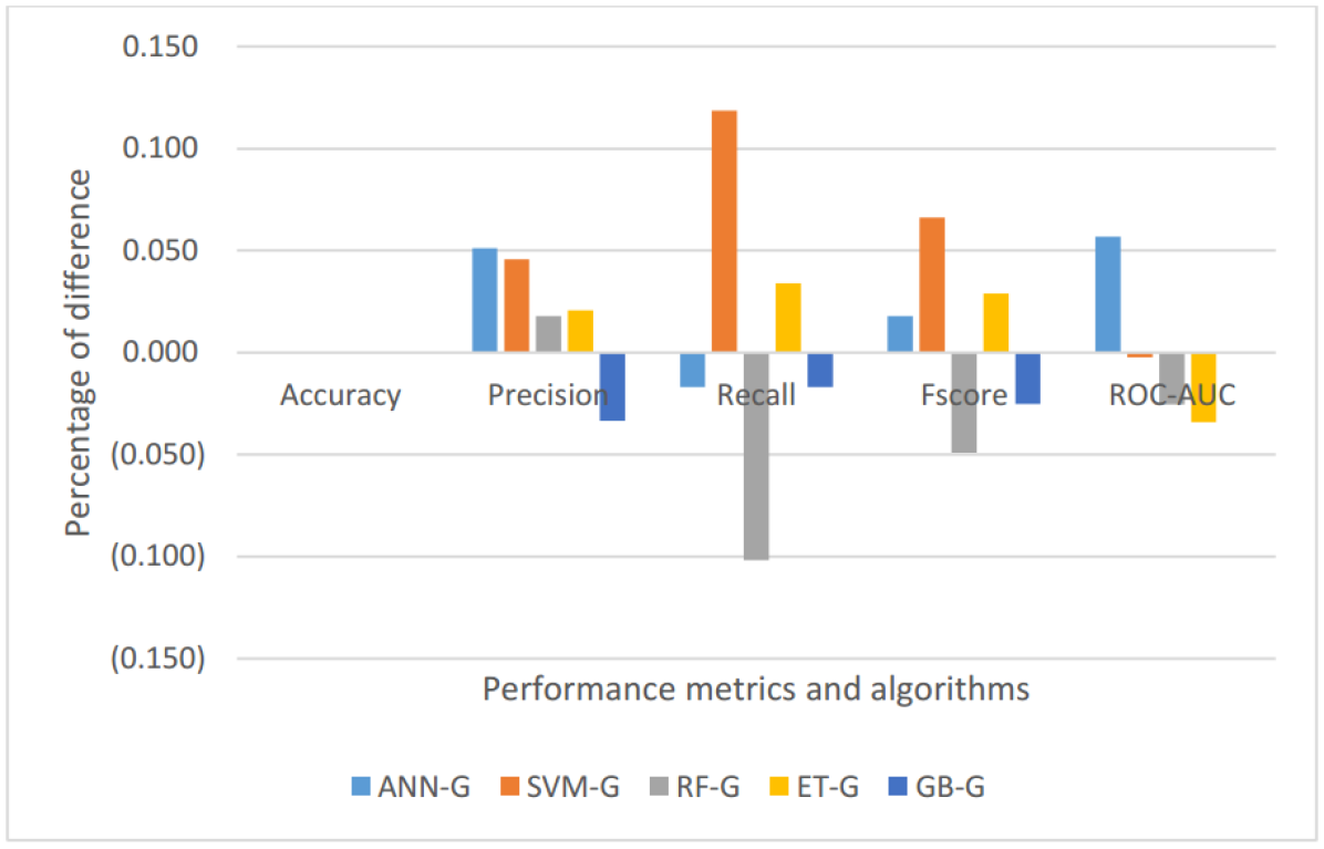
Figure 3. Dispersion in performance metrics for the case of using generalized frequent feature set

Furthermore, from Figure 4, we can also see that, for the most important performance metric recall, we are getting better performance (ranging from 2-10%) for ANN-G, RF-G, and GB-G. In terms of any performance metrics, there is at least one algorithm that performs better or equal using the generalized frequent feature. We need to choose the right algorithm based on the class distribution in the data as performance metric response differs based upon the distribution of the class in the data. Furthermore, when we use the generalized feature sets, we run the algorithm on all 25 generalized feature sets to discover the best feature sets. We found that using frequent feature set # 5 (see Table 4), out of the 25 generalized feature sets, for algorithms RF-G, ET-G, and GB-G we are able to achieve the best result based on performance metric recall. For ANN-G and SVM-G, pattern 3 and 6 worked better accordingly. Therefore, this helps to choose the best generalized frequent feature set for a particular algorithm among many generalized frequent feature sets.

We only tested with the Freddie Mac dataset and there is a chance that the original features (even after excluding unnecessary features using the feature selection technique) still overfit the model, which leads to a better or equal result for all performance metrics in our case. Validating the result with multiple datasets is part of the future direction of this work. Furthermore, overall, all algorithms using a generalized frequent feature set takes less execution time compared to their counterparts due to the much fewer number of features. For a few algorithms (e.g., ANN), a fewer number of features decreases the computation time.

Overall, even though infusing domain knowledge might lead to some compromise in performance, clearly it ensures better explainability and interpretability as the output is made from a concise and familiar set of features from the domain. Our success so far is in the generation of the output using an intuitive set of features. Our further concern is to show the result in an interpretable way. One way is by expressing the output as a percentage of the total risk, and the segregation of the output value is the percentage that each of the generalized frequent features is liable. We can express the total risk probability with the following formula:

(1) $$P(D)=\sum_{g=0}^{G}contribution(g)$$

where g is the generalized frequent feature. Instead of using contributions from generalized frequent features, we can also express the output in terms of the contribution from each element of the domain concept. This might improve the interpretability a little bit at the expense of losing some details.

The correct way to come up with the breakdown of contribution from each feature for a particular prediction contribution is challenging. The naive way to formulate this can be by using the importance or permutation importance of the features. However, the importance of the feature is usually calculated based on a set of data (e.g., training set) and can be achieved directly from feature importance methods in most supervised algorithms. However, in case of sample wise feature importance this is not for straight forward. Moreover, the test sample might not be a good representative of the training set. Other work such as LIME (Ribeiro et al., 2016), Tree Interpreter (Ando, [n. d.]), SHAP (Lundberg and Lee, 2017), and ELI5 (on_, [n. d.]b), can discover the contributions of features in the prediction. However, each of the available techniques/tools come with some limitations: some are applicable to only text or images individually, and some are applicable to only a class of algorithms (e.g., tree based approaches, neural networks). Most of these approaches try to find out how the prediction deviates from the base/average scenario. Lime (Ribeiro et al., 2016) tries to generate an explanation by locally (i.e., using local behavior) approximating the model with an interpretable model (e.g., decision trees, linear model). However, it is limited by the use of a linear model to approximate local behavior.Furthermore, SHAP unifies previous approaches including LIME by borrowing features from those. While SHAP comes with theoretical guarantees about consistency and local accuracy from game theory, in the case of black box kernel SHAP, it needs to run many evaluations of the original model to estimate a single vector of feature importance (sha, [n. d.]). ELI5 also uses the LIME algorithm internally for explanations, however, the model is not truly agnostic, mostly limited to tree-based and other parametric or linear models. Tree Interpreter is limited to only tree-based approaches (e.g., Random Forest, Decision Trees). Our future work includes finding an optimal solution for sample-wise feature contribution in the prediction and express the sample-wise output according to the formula 1.

6. Conclusions and future work

Future adoption of ”black box” models is in an inauspicious position due to the lack of explainability. Governments of different countries have started to introduce laws to ensure accountability, right of explanation, and eliminating bias/discrimination in decisions. Sophisticated areas such as finance, security, and healthcare are in need of better explanations of their ”black box” models. In this work, we demonstrated a way to collect and use domain knowledge from the literature. We also introduced a way to bring and infuse popular concepts (e.g., 5 C’s of credit) from the literature that aide in better interpretability and explainability. Our experimental results show that ”black box” models can be better explainable without much compromise in performance when domain knowledge is infused.

Experimenting with our proposed approach on multiple data sets will help us validate its versatility. Moreover, finding an optimal solution to segregate the contribution of each participating feature (sample wise) will aide in better explainability of sample wise output and better run-time of the model. In addition, incorporating other concepts as domain knowledge will verify its generality, making this approach transferable to other domains like cyber-security and healthcare. For instance, in cyber-security, better explanation would aide in the understanding of different attack scenarios and safeguarding the model from adversarial attacks.

- (1)
- alg ([n. d.]) [n. d.]. Algorithmic Accountability. Retrieved April 20, 2019 from https://www.wyden.senate.gov/imo/media/doc/Algorithmic%20AccountabilityAct%20of%202019%20Bill%20Text.pdf
- on_([n. d.]a) [n. d.]a. Apriori mlxtend. Retrieved April 20, 2019 from http://rasbt.github.io/mlxtend/user_guide/frequent_patterns/apriori
- rev ([n. d.]) [n. d.]. black-box-explainability. Retrieved May 7, 2019 from https://github.com/SheikhRabiul/black-box-explainability/blob/master/feature_generalizer/literature_review.csv
- pro ([n. d.]) [n. d.]. black-box-explainability. Retrieved May 7, 2019 from https://github.com/SheikhRabiul/black-box-explainability
- on_([n. d.]b) [n. d.]b. ELI5. Retrieved April 29, 2019 from https://eli5.readthedocs.io/en/latest/overview.html
- ens ([n. d.]) [n. d.]. Ensemble methods. Retrieved April 23, 2019 from https://scikit-learn.org/stable/modules/ensemble.html
- exp ([n. d.]) [n. d.]. Explainable AI. Retrieved May 7, 2019 from https://www.darpa.mil/program/explainable-artificial-intelligence
- on_([n. d.]c) [n. d.]c. Explainable Artificial Intelligence. Retrieved April 20, 2019 from https://www.kdnuggets.com/2019/01/explainable-ai.html
- 5cs ([n. d.]) [n. d.]. Five Cs of Credit. Retrieved April 20, 2019 from https://www.investopedia.com/terms/f/five-c-credit.asp
- sci ([n. d.]) [n. d.]. Scikit-learn: Machine Learning in Python. Retrieved May 7, 2019 from https://scikit-learn.org/stable/
- sha ([n. d.]) [n. d.]. SHAP vs LIME. Retrieved May 7, 2019 from https://github.com/slundberg/shap/issues/19
- fre ([n. d.]) [n. d.]. Single Family Loan Level Dataset - Freddie Mac. Retrieved May 7, 2019 from http://www.freddiemac.com/research/datasets/sf_loanlevel_dataset.page
- ten ([n. d.]) [n. d.]. Tensorflow. Retrieved May 7, 2019 from https://www.tensorflow.org/
- Agrawal et al. (1994) Rakesh Agrawal, Ramakrishnan Srikant, et al. 1994. Fast algorithms for mining association rules. In Proc. 20th int. conf. very large data bases, VLDB, Vol. 1215. 487–499.
- Alaka et al. (2018) Hafiz A Alaka, Lukumon O Oyedele, Hakeem A Owolabi, Vikas Kumar, Saheed O Ajayi, Olugbenga O Akinade, and Muhammad Bilal. 2018. Systematic review of bankruptcy prediction models: Towards a framework for tool selection. Expert Systems with Applications 94 (2018), 164–184.
- Alfaro and Gallardo (2012) Rodrigo Alfaro and Natalia Gallardo. 2012. The determinants of household debt default. (2012).
- Anderson and Jozwik (2014) Scott Anderson and Janet Jozwik. 2014. Building a Credit Model Using GSE Loan-Level Data. Journal of Structured Finance 20, 1 (2014), 19.
- Ando ([n. d.]) Saabas Ando. [n. d.]. Interpreting random forests. Retrieved April 29, 2019 from http://blog.datadive.net/interpreting-random-forests/
- Angelini et al. (2008) Eliana Angelini, Giacomo di Tollo, and Andrea Roli. 2008. A neural network approach for credit risk evaluation. The quarterly review of economics and finance 48, 4 (2008), 733–755.
- Antinolfi et al. (2016) Gaetano Antinolfi, Celso Brunetti, and Jay Im. 2016. Mortgage rates and credit risk: Evidence from mortgage pools. Available at SSRN 2809367 (2016).
- Bach et al. (2015) Sebastian Bach, Alexander Binder, Grégoire Montavon, Frederick Klauschen, Klaus-Robert Müller, and Wojciech Samek. 2015. On pixel-wise explanations for non-linear classifier decisions by layer-wise relevance propagation. PloS one 10, 7 (2015), e0130140.
- Bellovary et al. (2007) Jodi L Bellovary, Don E Giacomino, and Michael D Akers. 2007. A review of bankruptcy prediction studies: 1930 to present. Journal of Financial education (2007), 1–42.
- Berka (2016) P Berka. 2016. Using the LISp-Miner System for Credit Risk Assessment. Neural Network World 26, 5 (2016), 497.
- Bhattacharya et al. (2019) Arnab Bhattacharya, Simon P Wilson, and Refik Soyer. 2019. A Bayesian approach to modeling mortgage default and prepayment. European Journal of Operational Research 274, 3 (2019), 1112–1124.
- Boser et al. (1992) Bernhard E Boser, Isabelle M Guyon, and Vladimir N Vapnik. 1992. A training algorithm for optimal margin classifiers. In Proceedings of the fifth annual workshop on Computational learning theory. ACM, 144–152.
- Bradley et al. (2015) Michael G Bradley, Amy Crews Cutts, and Wei Liu. 2015. Strategic mortgage default: The effect of neighborhood factors. Real Estate Economics 43, 2 (2015), 271–299.
- Breiman (2001) Leo Breiman. 2001. Random forests. Machine learning 45, 1 (2001), 5–32.
- Chan et al. (2016) Sewin Chan, Andrew Haughwout, Andrew Hayashi, and Wilbert Van der Klaauw. 2016. Determinants of mortgage default and consumer credit use: the effects of foreclosure laws and foreclosure delays. Journal of Money, Credit and Banking 48, 2-3 (2016), 393–413.
- Chandrasekaran et al. (1989) B Chandrasekaran, Michael C Tanner, and John R Josephson. 1989. Explaining control strategies in problem solving. IEEE Intelligent Systems 1 (1989), 9–15.
- Datta et al. (2016) Anupam Datta, Shayak Sen, and Yair Zick. 2016. Algorithmic transparency via quantitative input influence: Theory and experiments with learning systems. In 2016 IEEE symposium on security and privacy (SP). IEEE, 598–617.
- Demiroglu et al. (2014) Cem Demiroglu, Evan Dudley, and Christopher M James. 2014. State foreclosure laws and the incidence of mortgage default. The Journal of Law and Economics 57, 1 (2014), 225–280.
- Elul et al. (2010) Ronel Elul, Nicholas S Souleles, Souphala Chomsisengphet, Dennis Glennon, and Robert Hunt. 2010. What” triggers” mortgage default? American Economic Review 100, 2 (2010), 490–94.
- Fang et al. (2016) Hanming Fang, You Kim, and Wenli Li. 2016. The dynamics of subprime adjustable-rate mortgage default: a structural estimation. (2016).
- Fitzpatrick and Mues (2016) Trevor Fitzpatrick and Christophe Mues. 2016. An empirical comparison of classification algorithms for mortgage default prediction: evidence from a distressed mortgage market. European Journal of Operational Research 249, 2 (2016), 427–439.
- Foote and Willen (2018) Christopher L Foote and Paul S Willen. 2018. Mortgage-default research and the recent foreclosure crisis. Annual Review of Financial Economics 10 (2018), 59–100.
- Fout et al. (2018) Hamilton Fout, Grace Li, Mark Palim, and Ying Pan. 2018. Credit risk of low income mortgages. Regional Science and Urban Economics (2018).
- Friedman (2001) Jerome H Friedman. 2001. Greedy function approximation: a gradient boosting machine. Annals of statistics (2001), 1189–1232.
- Geurts et al. (2006) Pierre Geurts, Damien Ernst, and Louis Wehenkel. 2006. Extremely randomized trees. Machine learning 63, 1 (2006), 3–42.
- Ghent and Kudlyak (2011) Andra C Ghent and Marianna Kudlyak. 2011. Recourse and residential mortgage default: evidence from US states. The Review of Financial Studies 24, 9 (2011), 3139–3186.
- Goodman and Flaxman (2017) Bryce Goodman and Seth Flaxman. 2017. European Union regulations on algorithmic decision-making and a “right to explanation”. AI Magazine 38, 3 (2017), 50–57.
- Goodman et al. (2014) Laurie S Goodman, Brian Landy, Roger Ashworth, and Lidan Yang. 2014. A Look at Freddie Mac’s Loan-Level Credit Performance Data. Journal of Structured Finance 19, 4 (2014), 52.
- Greenwald (2018) Daniel Greenwald. 2018. The mortgage credit channel of macroeconomic transmission. (2018).
- Gyourko and Tracy (2014) Joseph Gyourko and Joseph Tracy. 2014. Reconciling theory and empirics on the role of unemployment in mortgage default. Journal of Urban Economics 80 (2014), 87–96.
- Hooman et al. (2016) Alireza Hooman, Govindan Marthandan, Wan Fadzilah Wan Yusoff, Mohana Omid, and Sasan Karamizadeh. 2016. Statistical and data mining methods in credit scoring. The Journal of Developing Areas 50, 5 (2016), 371–381.
- Islam (2018) Sheikh Rabiul Islam. 2018. An efficient technique for mining bad credit accounts from both olap and oltp. Ph.D. Dissertation. Tennessee Technological University.
- Islam et al. (2018a) Sheikh Rabiul Islam, William Eberle, and Sheikh Khaled Ghafoor. 2018a. Credit default mining using combined machine learning and heuristic approach. arXiv preprint arXiv:1807.01176 (2018).
- Islam et al. (2018b) Sheikh Rabiul Islam, Sheikh Khaled Ghafoor, and William Eberle. 2018b. Mining Illegal Insider Trading of Stocks: A Proactive Approach. In 2018 IEEE International Conference on Big Data (Big Data). IEEE, 1397–1406.
- Karamon et al. (2017) Kadiri Karamon, Douglas McManus, and Jun Zhu. 2017. Refinance and Mortgage Default: A Regression Discontinuity Analysis of HARP’s Impact on Default Rates. The Journal of Real Estate Finance and Economics 55, 4 (2017), 457–475.
- Khandani et al. (2010) Amir E Khandani, Adlar J Kim, and Andrew W Lo. 2010. Consumer credit-risk models via machine-learning algorithms. Journal of Banking & Finance 34, 11 (2010), 2767–2787.
- Kim et al. (2018) You Suk Kim, Steven M Laufer, Richard Stanton, Nancy Wallace, and Karen Pence. 2018. Liquidity crises in the mortgage market. Brookings Papers on Economic Activity 2018, 1 (2018), 347–428.
- Kvamme et al. (2018) Håvard Kvamme, Nikolai Sellereite, Kjersti Aas, and Steffen Sjursen. 2018. Predicting mortgage default using convolutional neural networks. Expert Systems with Applications 102 (2018), 207–217.
- Lei et al. (2016) Tao Lei, Regina Barzilay, and Tommi Jaakkola. 2016. Rationalizing neural predictions. arXiv preprint arXiv:1606.04155 (2016).
- Lipovetsky and Conklin (2001) Stan Lipovetsky and Michael Conklin. 2001. Analysis of regression in game theory approach. Applied Stochastic Models in Business and Industry 17, 4 (2001), 319–330.
- Lipton (2016) Zachary C Lipton. 2016. The mythos of model interpretability. arXiv preprint arXiv:1606.03490 (2016).
- Liu and Sing (2018) Bo Liu and Tien Foo Sing. 2018. “Cure” Effects and Mortgage Default: A Split Population Survival Time Model. The Journal of Real Estate Finance and Economics 56, 2 (2018), 217–251.
- Low (2015) David Low. 2015. Mortgage default with positive equity. Job Market Paper, New York University (2015).
- Lundberg and Lee (2017) Scott M Lundberg and Su-In Lee. 2017. A unified approach to interpreting model predictions. In Advances in Neural Information Processing Systems. 4765–4774.
- Miller (2018) Tim Miller. 2018. Explanation in artificial intelligence: Insights from the social sciences. Artificial Intelligence (2018).
- Moulton et al. (2016) Stephanie Moulton, Donald Haurin, Wei Shi, et al. 2016. Reducing default rates of reverse mortgages. Issue in Brief 16 11 (2016).
- Ribeiro et al. (2016) Marco Tulio Ribeiro, Sameer Singh, and Carlos Guestrin. 2016. Why should i trust you?: Explaining the predictions of any classifier. In Proceedings of the 22nd ACM SIGKDD international conference on knowledge discovery and data mining. ACM, 1135–1144.
- Shrikumar et al. (2017) Avanti Shrikumar, Peyton Greenside, and Anshul Kundaje. 2017. Learning important features through propagating activation differences. In Proceedings of the 34th International Conference on Machine Learning-Volume 70. JMLR. org, 3145–3153.
- Sirignano and Giesecke (2018) Justin Sirignano and Kay Giesecke. 2018. Risk analysis for large pools of loans. Management Science 65, 1 (2018), 107–121.
- Sirignano et al. (2016) Justin Sirignano, Apaar Sadhwani, and Kay Giesecke. 2016. Deep learning for mortgage risk. arXiv preprint arXiv:1607.02470 (2016).
- Sorenson (2015) David J Sorenson. 2015. Loan Characteristics, Borrower Traits, and Home Mortgage Foreclosures: The Case of Sioux Falls, South Dakota. Journal of Regional Analysis and Policy 45, 1100-2016-90130 (2015), 163.
- SOUSA et al. (2015) MR SOUSA, J GAMA, and E BRANDÃO. 2015. Stress-testing the return on lending under real extreme adverse circumstances. In European Financial Management Association annual conference. Amsterdam: EFMA.
- Sousa et al. (2015) Maria Rocha Sousa, João Gama, and Elísio Brandão. 2015. Links between Scores, Real Default and Pricing: Evidence from the Freddie Mac’s Loan-level Dataset. Journal of Economics, Business and Management 3, 12 (2015), 1106–1114.
- Sousa et al. (2016) Maria Rocha Sousa, João Gama, and Elísio Brandão. 2016. A new dynamic modeling framework for credit risk assessment. Expert Systems with Applications 45 (2016), 341–351.
- Štrumbelj and Kononenko (2014) Erik Štrumbelj and Igor Kononenko. 2014. Explaining prediction models and individual predictions with feature contributions. Knowledge and information systems 41, 3 (2014), 647–665.
- Swartout (1985) William R Swartout. 1985. Rule-based expert systems: The mycin experiments of the stanford heuristic programming project: BG Buchanan and EH Shortliffe,(Addison-Wesley, Reading, MA, 1984); 702 pages.
- Swartout and Moore (1993) William R Swartout and Johanna D Moore. 1993. Explanation in second generation expert systems. In Second generation expert systems. Springer, 543–585.
- Tian et al. (2016) Chao Yue Tian, Roberto G Quercia, and Sarah Riley. 2016. Unemployment as an adverse trigger event for mortgage default. The Journal of Real Estate Finance and Economics 52, 1 (2016), 28–49.
- Wilson and Sharda (1994) Rick L Wilson and Ramesh Sharda. 1994. Bankruptcy prediction using neural networks. Decision support systems 11, 5 (1994), 545–557.
- Wu and Dorfman (2018) Yifei Wu and Jeffrey H Dorfman. 2018. Reducing residential mortgage default: Should policy act before or after home purchases? PloS one 13, 7 (2018), e0200476.
- Yang and Shafto (2017) Scott Cheng-Hsin Yang and Patrick Shafto. 2017. Explainable Artificial Intelligence via Bayesian Teaching. In NIPS 2017 workshop on Teaching Machines, Robots, and Humans.