Distinguishing noisy boson sampling from classical simulations
Valery Shchesnovich
valery@ufabc.edu.brCentro de Ciências Naturais e Humanas, Universidade Federal do
ABC, Santo André, SP, 09210-170 Brazil
Abstract
Giving a convincing experimental evidence of the quantum supremacy over classical simulations is a challenging goal. Noise is considered to be the main problem in such a demonstration, hence it is urgent to understand the effect of noise. Recently found classical algorithms can efficiently approximate, to any small error, the output of boson sampling with finite-amplitude noise. In this work it is shown analytically and confirmed by numerical simulations that one can efficiently distinguish the output distribution of such a noisy boson sampling from the approximations accounting for low-order quantum multiboson interferences, what includes the mentioned classical algorithms. The number of samples required to tell apart the quantum and classical output distributions is strongly affected by the previously unexplored parameter: density of bosons, i.e., the ratio of total number of interfering bosons to number of input ports of interferometer. Such critical dependence is strikingly reminiscent of the quantum-to-classical transition in systems of identical particles, which sets in when the system size scales up while density of particles vanishes.
1 Introduction
Quantum mechanics promises computational advantage over digital computers [F, Sh]. Current technology is on the brink of building quantum devices with the promised advantage in some specific computational tasks, called the quantum supremacy [P], for which goal several quantum systems are considered [AA, QSProp, QSArch, QSChar, QSColdAt] and a dramatic breakthrough was recently reported [GoogleS]. Can noise, always present in an experimental setup, compromise the quantum supremacy by allowing for an efficient classical simulation [HQCF]? In this work we consider how a noisy boson sampling system can be distinguished from efficient classical approximations.
In boson sampling proposal of Aaronson & Arkhipov [AA] the specific classically hard computational task is sampling from many-body quantum interference of indistinguishable bosons on a unitary linear -dimensional interferometer. At least in the so-called no-collision regime, when the output ports receive at most a singe boson (i.e., for [Bbirthday]), complexity-theoretic arguments have been found in Ref. [AA] for the quantum advantage over classical simulations. In general, the output probabilities depend on the full many-body quantum interference of bosons given by a sum of quantum amplitudes, i.e., by the matrix permanents [C, Scheel], which are hard to compute [Valiant, JSV, A1, Ryser].
The boson sampling proposal had initiated efforts for experimental demonstration. Single photons [E1, E2, E3, E4, EVCC] as well as Gaussian states [GBS, E5, GSNEW] in optical interferometers, and the temporal-mode encoding [TbinBS, TbinBSExp] were proposed and tested for experimental implementation with quantum optics. Experimental quantum optical platform has seen significant advances [pure1phBS, HEBS, LossBS, 12phBS] culminating recently in an experimental implementation with 20 photons on a 60-mode interferometer [20ph60mod]. Alternative platforms include ion traps [BSions], superconducting qubits [BSsuperc, Goldstein], neutral atoms in optical lattices [BSoptlatt] and dynamic Casimir effect [BScas]. Initial estimate on the threshold size for demonstration of quantum supremacy with boson sampling was bosons [AA]. However, recent classical simulations [QSBS, Cliffords] pushed the threshold to bosons. Inevitable experimental noise [Goldstein, RR, KK, LP, VS14, Arkh, Brod, Latm] additionally opens possibilities for efficient classical approximation algorithms [K1, R1, OB, PRS, RSP, VS2019, NonUnifLoss]. Most importantly, if noise amplitudes do not vanish when the system size scales up, the recent algorithms of Refs. [R1, RSP, VS2019] approximate efficiently the output distribution of noisy boson sampling by low-order multi-boson interference.
Unavoidable noise has been accounted for in the boson sampling proposal [AA] by allowing for an approximation error. Taking into account that the complexity-theoretic arguments for the quantum supremacy are asymptotic, whereas in an experiment one has a finite quantum device, one may wonder how small experimental error should be? In the spirit of Ref. [F], the experimental error problem can be formulated as follows: Can a classical algorithm efficiently sample from the output distribution of a quantum device in such a way that it would be impossible to tell from the sampling data whether we have the classical simulation or the quantum device? At the other extreme, the two output distributions can be efficiently distinguished. Since the promised computational advantage is due to the opening gap between exponential and polynomial computations in the size of a quantum system [P], it is reasonable to consider a method of distinguishing a quantum device from a classical simulation as efficient if it requires only a polynomial in the quantum system size number of samples.
As a partial answer to the above problem, in the present work it is shown that one can efficiently distinguish the output distribution of noisy boson sampling from output distributions of a wide range of classical algorithms, such as simulation with classical particles and the recent algorithms of Refs. [R1, RSP, VS2019]. We give an analytical expression for the lower bound on the total variation distance between the output distribution of noisy boson sampling and that of such a classical simulation and point that the probability of no particle counts in a subset of output ports can be used for distinguishing the quantum and classical distributions. The number of samples necessary for distinguishing the quantum and classical distributions critically depends on the density of bosons, defined as the ratio of the total number of interfering bosons to the number of input ports of interferometer, and not on the number of bosons or the number of ports of interferometer themselves. Our analytical results are valid asymptotically with the number of interfering bosons, convergence to the asymptotic result is studied by using numerical simulations.
Previously the output distribution of boson sampling was shown [BSNotUn] to be far in the total variation distance from the uniform distribution (argued to be an efficient approximation [BSUn]), where a set of open problems was given. The present work partially resolves open problems (2) and (4)-(6) of Ref. [BSNotUn] by considering a wide class of possible classical approximations to a noisy realization of boson sampling with arbitrary scaling of the interferometer size in the total number of interfering bosons, beyond the no-collision regime. In Ref. [BB] it was shown how one can efficiently distinguish the output distribution of boson sampling from the simulation by classical particles. Statistical or pattern recognition techniques were also applied to assessment of boson sampling and distinguishing it from classical simulations [StatBench, ExpStatSign, WDBubles, PatternRec]. However, no analysis of the impact of realistic experimental noise was attempted previously, which is the main goal of the present work.
The text is organized as follows. In section 2 the boson sampling realization with linear optics and the classical approximations by low-order multi-boson interference are described and our results on distinguishing their respective output probability distributions are presented. In section 3 our principal findings are summarized and discussed. For better readability, the derivations and mathematical details are relegated to Appendices A-LABEL:appF.
2 Noisy boson sampling vs classical approximations
The boson sampling proposal of Ref. [AA] considers the quantum interference of identical single bosons on a unitary -port in the no-collision regime , here we consider it for arbitrary . It turns out that distinguishing noisy boson sampling, as scales up, crucially depends on density of bosons
, more precisely, on the scaling (or, equivalently, ). This fact allows us to consider all models with a given scaling as a class of boson sampling, where serves as the size parameter in the class. For example, for at least we have the so-called no-collision regime, the main focus of Ref. [AA].
Let us now mention known estimates on the number of classical computations required to simulate the boson sampling. For the ideal (noiseless) boson sampling, the fastest to date algorithms of Refs. [QSBS, Cliffords] can sample from its output distribution in computations. The number of computations depends on the density of bosons: for non-vanishing density of bosons the output probabilities can be given by the matrix permanents of rank-deficient matrices with reduced computational complexity [Barv, CompHard]. The following simple rule can be stated [MyEst]: to sample from the boson sampling in arbitrary regime of density of bosons by the algorithm of [Cliffords] requires at least as many classical simulations as for the no-collision boson sampling with bosons. The size parameter gives also the expected number of output ports occupied by bosons as a function of the boson density.
Less is known about the scaling of classical computations for exact sampling from noisy boson sampling. There are several strong sources of noise: noisy interferometer [LP, Arkh], partial distinguishability of bosons [VS14], and boson losses [Brod, Latm]. It was shown that a finite number of lost bosons (or dark counts of detectors, or both) does not compromise the computational hardness of boson sampling in the no-collision regime. There are also results for the approximate sampling from noisy boson sampling, where the number of classical computations depends additionally on the scaling of the amplitude of noise in the system size [KK, R1, RSP, VS2019]. Efficient classical approximation algorithm of boson sampling in the no-collision regime with partially distinguishable bosons was found in Ref. [R1], then extended to losses [RSP] and noise in interferometer [VS2019]. For intermediate-size boson sampling devices the number of computations of the classical algorithm can be further optimized [MRRT]. There is equivalence of different imperfections in their effect on classical hardness of boson sampling, e.g., noise in experimental platforms [EVCC, Goldstein] has a similar effect to that of the partial distinguishability of bosons [VS2019] (below we will use the term noise for all imperfections).
The efficient classical algorithm of Refs. [R1, RSP, VS2019] can approximate the output distribution of -boson sampling with a finite-amplitude noise by a smaller one, with interfering bosons and classical particles, it becomes efficient (i.e., polynomial in ) for bounded , since the classical computations scale exponentially only in [R1]. Below we investigate if a noisy boson sampling with finite-amplitude noise can be efficiently distinguished from such a classical approximation, to answer the experimentally relevant problem posed in the previous section.
Probability distribution at output of noisy boson sampling
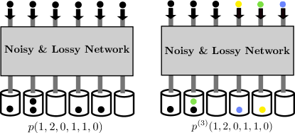
Let us now briefly describe an experimental implementation of boson sampling. We will use the popular example of linear optical setup with single photons, see fig. 1, and focus on two sources of noise: losses of photons and their partial distinguishability. Later on, we will include also the false random (a.k.a. dark) counts of detectors, i.e., the counts which are not triggered by photons. There is an equivalence of the losses compensated by dark counts with noise in the interferometer [VS2019], thus our model takes into account the strongest sources of noise in linear optical experimental setup. The multi-photon component at input is neglected here. It can be a strong source of noise with the photon sources based on the parametric down conversion, e.g., when about sources are used to produce single photons in the boson sampling from a Gaussian state [GBS, E5, 12phBS]. With additional optical multiplexing of the sources one can significantly reduce the multiphoton component noise [S2020].
Figure 1: Noisy boson sampling vs classical approximation. Noisy -boson quantum interference on a -port (left). An adversary (right) tries to approximate the output distribution of -boson quantum interference, , by the output distribution, , from a combination of -boson interference (here ) and distinguishable bosons.
Unitary linear optical interferometer with input and output ports connects the optical mode of input port to the optical modes of the output ports: . Such an interferometer would take a Fock state of photons in the input ports into a superposition of the Fock states of the photons in the output ports according to the corresponding input-output relations between the boson creation operators in the input and output ports:
(1)
where () is the boson creation operator in input (output) port (). The (photon number-resolving) photon detection projects the output state of photons onto one of the Fock states in the output ports. A realistic optical setup, however, suffers from photon losses and not all the photons are detected. Ways to compensate for losses, such as by the post selection on a given number of photons [LossBS], are currently under investigation. For boson sampling one can allow only a constant number of bosons to be lost [Brod]. On the other hand, if we assume that photons are lost independently of each other, there will be, on average, a proportional to number of lost photons. The classical algorithm of Ref. [RSP] can efficiently approximate the output distribution with the proportional losses. The post selection strategy therefore can work only for a small-size boson sampling, since the probability to lose a constant number of photons vanishes exponentially with . Thus photon losses are unavoidable source of noise in an optical realization of boson sampling. The input-output relation in the case of arbitrary lossy interferometer , can be cast in the following form [LossNet]
(2)
where is the boson creation operator in loss mode (e.g., photon absorption due to non-unitarity of an interferometer), and matrix is such that the total unitarity is observed (see more details in appendix B).
Another strong source of noise is partial distinguishability of photons, affecting the output state of photons on a linear interferometer [HOM]. Partial distinguishability can be associated with different internal states of photons (such as temporal profile of a photon in case of Ref. [HOM]), which are unaffected by the input-output relation in Eq. (2) and not resolved in an experiment. In this case, the boson operators in the input-output relations of Eq. (2) refer to the same internal state of boson on the input as well as on the output of the interferometer. Partial distinguishability of bosons can be accounted for by introducing a function on permutations , acting on the internal states of bosons [VS14, PartDist]. This function is defined as follows. For pure internal states of bosons, , , it reads
(3)
For mixed internal states is a convex sum of the products as in Eq. (3). Note that of Eq. (3) factorizes according to the disjoint cycle decomposition of permutation [Stanley], where each cycle ( denotes the cycle length) contributes a factor given by a similar expression as the right hand side of Eq. (3) with replaced by . In general, each cycle-factor accounts for a specific -boson interference process [Ninter] and the factorization of occurs when bosons are uncorrelated, i.e., when their internal state is factorized . For instance, in the famous -photon interference experiment [HOM], for the transposition of the photons (i.e., -cycle ) we have
, with being the temporal shape of photon . This value enters the probability of the coincidence count at the output of a unitary linear -port: , i.e., the Mandel dip in Ref. [HOM] (more on the partial distinguishability can be found in Ref. [PartDist]). Explicit analytical results below are obtained for the uniform partial distinguishability, controlled by a single distinguishability parameter . This model applies when boson with probability is in some pure internal state and with probability in an unique internal state , orthogonal to all other internal states. Either pure or mixed state of boson may correspond to such a case:
For bosons in internal states of Eq. (2), each -cycle for contributes the factor to the distinguishability function in Eq. (3). The sum of all the cycle lengths in a permutation satisfies , where is the number of fixed points (-cycles), hence . If photon detectors do not resolve the internal states of photons, the same distinguishability function corresponds to pure-state or mixed-state model in Eq. (2). In an experiment, there is always noise in photon parameters, such as random fluctuations of photon arrival times, thus the internal states of photons are always mixed. Whatever is the model of photon detection, the distinguishability of photons due to mixed states will persist, since even by completely resolving the internal states of photons one is not able to affect the distinguishability coming from the fluctuations of photon parameters [VS2020]. Thus partial distinguishability of photons is a source of unavoidable noise in boson sampling experiments with photons.
We can now give the output distribution of our noisy boson sampling model with boson losses and partially distinguishable bosons. When bosons, with the distinguishability function , are sent to the input ports of a lossy interferometer , the probability to detect exactly of them, , at the output ports in a configuration , , i.e., when bosons are detected at output port , reads (see appendix B for details)
(7)
where the sum over stands for summation over all -dimensional subsets of , the multi-set contains the output ports with bosons (one for each detected boson) and .
When only bosons are detected at the output, there is still some interference between the lost bosons and the detected ones, reflected in exchange of bosons between the output and the loss modes by permutation in Eq. (7). Only for a diagonal loss matrix no such boson exchange occurs (in this case for all ) and the residual interference disappears. In the latter case, boson losses can be considered to occur, e.g., at the input of the interferometer [PRS] and there is such , , that for some . Parameter in this case is the probability that boson sent to input port actually passes the interferometer (i.e., is the probability that boson is lost). Below, some of our explicit results are given for the uniform loss model with , , where is the uniform transmission of such an interferometer.
Approximations by interfering bosons and classical particles
In the no-collision regime, the output distribution of noisy -boson sampling model can be approximated, to any small error, by a similar noisy model with bosonic particles, where there are only interfering bosons and the rest particles are distinguishable bosons (i.e., classical particles) [R1, RSP, VS2019]. The parameter is chosen according to the required approximation error. Below we adopt such a classical approximation as the classical adversary, see fig. 1.
The simplest way to introduce the above described classical approximation is via the respective distinguishability function , which is equal to for permutations with at least fixed points and to zero otherwise [VS2019]:
(8)
With such a distinguishability function, for , randomly chosen bosons contribute to the output probability in the same way as classical particles, whereas the rest bosons are allowed to interfere. By setting or we get classical particles (since a permutation with fixed points is the identity permutation).
Our goal is to estimate the total variation distance between the output distributions of noisy boson sampling () and a classical approximation (), where both distributions are given by Eq. (7) with the corresponding distinguishability functions and . The total variation distance is defined as follows
(9)
where the sum runs over all possible configurations of bosons in the output ports. The key observation is that for any subset of the configurations of bosons
in the output ports we have
(10)
Observe that the equality is necessarily achieved for a certain subset
depending on and other parameters of the setup.
Analytical analysis below is carried out for the difference in probability, , of all the output bosons to be detected in a subset of output ports, or, equivalently, no particle counts in the complementary subset of the output ports . Let us assume that such a subset is chosen once for a given setup (below we will return to this point in more detail). Since we consider arbitrary (or randomly chosen multiports) we will use in our analytical and numerical considerations below.
At this stage, the dark counts of detectors can be easily accounted for. Dark counts of a detector follow Poisson distribution , where we assume a uniform rate for all detectors. Hence, the dark counts contribute the factor to the the probability of no counts in output ports. Denoting we get from Eqs. (7)-(8) the following expression for the difference in probability of no counts in output ports (see details in appendices A and B)
Conversion to HTML had a Fatal error and exited abruptly. This document may be truncated or damaged.