Characterizing K2 Candidate Planetary Systems Orbiting Low-Mass Stars IV:
Updated Properties for 86 Cool Dwarfs Observed During Campaigns 1–17

Abstract

We present revised stellar properties for 172 K2 target stars that were identified as possible hosts of transiting planets during Campaigns 1–17. Using medium-resolution near-infrared spectra acquired with the NASA Infrared Telescope Facility/SpeX and Palomar/TripleSpec, we found that 86 of our targets were bona fide cool dwarfs, 74 were hotter dwarfs, and 12 were giants. Combining our spectroscopic metallicities with Gaia parallaxes and archival photometry, we derived photometric stellar parameters and compared them to our spectroscopic estimates. Although our spectroscopic and photometric radius and temperature estimates are consistent, our photometric mass estimates are systematically $\Delta M_{\star}=0.11{\rm\,M_{\odot}}$ (34%) higher than our spectroscopic mass estimates for the least massive stars ($M_{\star,phot}<0.4{\rm\,M_{\odot}}$). Adopting the photometric parameters and comparing our results to parameters reported in the Ecliptic Plane Input Catalog, our revised stellar radii are $\Delta R_{\star}=0.15{\rm\,R_{\odot}}$ ($40\%$) larger and our revised stellar effective temperatures are roughly $\Delta T_{\rm eff}=65$K cooler. Correctly determining the properties of K2 target stars is essential for characterizing any associated planet candidates, estimating the planet search sensitivity, and calculating planet occurrence rates. Even though Gaia parallaxes have increased the power of photometric surveys, spectroscopic characterization remains essential for determining stellar metallicities and investigating correlations between stellar metallicity and planetary properties.

1 Introduction

In 2013, the Kepler spacecraft was repurposed for the K2 mission: a survey for transiting planets in a series of observation fields along the ecliptic plane. For each “Campaign,” the K2 Guest Observer office solicited proposals for target stars from the community. The selected targets are therefore a conglomeration of stars chosen for a variety of science programs. Recognizing that the short duration of each K2 campaign (65–90 days) precluded the detection of most small, cool planets transiting Sunlike stars, many K2 proposers interested in those planets nominated stars believed to be cool dwarfs. Despite the short K2 observation periods, the smaller radii and lower temperatures of cool dwarfs permit the detection of multiple transits of potentially habitable planets. As noted by Huber et al. (2016), 41% of stars observed by K2 during Campaigns 1–8 were initially classified as cool dwarfs and K2 has already observed many more cool dwarfs than the primary Kepler mission: during Campaigns 0–14, K2 observed 50,159 potential cool dwarfs.

Due to the fast-paced nature of the K2 mission many of the proposed targets were not well-characterized prior to observation by K2. Accordingly, a variety of teams pursue ground-based characterization of K2 target stars after possible planets are detected. In this paper, we present revised characterizations for 172 K2 Objects of Interest (K2OIs). As in the first paper in this series (Dressing et al., 2017a), we use empirically-based relations (Newton et al., 2014, 2015; Mann et al., 2013a, 2014, 2015) to determine the properties of potential cool dwarfs.

All of our targets have initial characterizations from the K2 Ecliptic Plane Input Catalog (EPIC, Huber et al., 2016), a database containing photometry, kinematics, and stellar properties for stars in and near the fields targeted by K2. For the vast majority of stars, the parameters were estimated from photometry and proper motions by using the Galaxia galactic model (Sharma et al., 2011) and Padova isochrones (Girardi et al., 2000; Marigo & Girardi, 2007; Marigo et al., 2008) to generate mock realizations of each K2 field. Galaxia produces synthetic stellar catalogs based on the adopted galactic conditions and survey parameters. The baseline version uses the Besançon analytical model Robin et al. (2003) for the disk of the Milky Way and N-body models by Bullock & Johnston (2005) for the stellar halo. The Padova ischrones are an established set of models for stars with initial masses of $0.15{\rm\,M_{\odot}}<M_{\star}<7{\rm\,M_{\odot}}$ and a range of metallicities ($0.0004\leq Z\leq 0.03$). For Sun-like stars, the Padova models agree well with other models such as Yonsei-Yale models (Yi et al., 2003, 2004) and Dartmouth models (Dotter et al., 2008), but the Padova models predict lower luminosities for cooler stars.

In the EPIC, a subset of stars have slightly more accurate properties based on Hipparcos parallaxes (van Leeuwen, 2007) and spectroscopy from RAVE DR4 (Kordopatis et al., 2013), LAMOST DR1 (Luo et al., 2015), and APOGEE DR12 (Alam et al., 2015). Due to the reliance on Padova isochrones, Huber et al. (2016) cautioned that radius estimates for cool dwarfs may be up to 20% too small because the Padova isochrones are known to systematically underestimate the radii of cool dwarfs (Boyajian et al., 2012).

In Dressing et al. (2017a), we acquired and analyzed NIR spectra of 144 candidate cool dwarfs observed by K2 during Campaigns 1–7. We found that half of the candidate cool dwarfs were giant stars or hotter dwarfs. For the 72 stars classified as cool dwarfs, we determined their radii to be roughly $0.13{\rm\,R_{\odot}}$ (39%) larger than the estimates provided in the EPIC. Our cool dwarf sample included stars with spectral types of K3 to M4, stellar effective temperatures of 3276–4753K, and stellar radii of $0.19-0.78{\rm\,R_{\odot}}$.

Similarly, in Martinez et al. (2017) we refined the properties of 34 cool dwarfs using NIR spectra acquired using the SOFI spectrograph (Moorwood et al., 1998) at the New Technology Telescope and found a median radius difference of $0.15{\rm\,R_{\odot}}$ compared to the values in the EPIC. We saw no systematic difference between our revised temperatures and those estimated in the EPIC, which suggests that the problem is primarily due to the overly petite model radii. This could result from the underlying model assumptions of the Padova isochrones such as treatment of opacities, convection, magnetic fields, star spots, and other phenomena intrinsic to low-mass stars (e.g., Feiden & Chaboyer, 2012, 2013).

Our work is one of many complementary efforts to improve the characterization of planetary systems and target stars observed by K2. For instance, Wittenmyer et al. (2018) presented revised properties for 46 K2 target stars by obtaining high-resolution spectra with the HERMES multi-object spectrograph on the Anglo-Australian Telescope and Hirano et al. (2018) acquired AO imaging and optical spectra to characterize 16 planets orbiting 12 low-mass K2 target stars.

The overall goals of our multi-semester project are to characterize the set of cool dwarf planetary systems detected by the K2 mission and investigate the overall prevalence and properties of cool dwarf planetary systems. In Paper I (Dressing et al., 2017a), we established the project and characterized the first set of candidate cool dwarfs observed by our program. We then revised the properties of the associated planet candidates by combining our revised stellar characterizations with new fits of the K2 transit photometry (Dressing et al., 2017b, Paper II). In Paper III (Dressing et al., 2018), we focused on K2-55b, a surprisingly massive Neptune-sized planet for which we had refined the orbital ephemerides by observing an additional transit with Spitzer and measured the mass with Keck/HIRES. The next paper in this series (Dressing, Vanderburg et al., in prep) will present updated transit fits, false positive probabilities, and bulk properties for the planet candidates associated with the stars classified in this paper.

This paper is focused on the characterization of the second set of stars observed by our program: 172 candidate cool dwarfs identified as possible planet host stars based on data acquired during K2 campaigns 1–17. We characterize these stars using a combination of archival photometry, new spectroscopic observations obtained by our team, and recently released astrometric data from Gaia DR2 (Gaia Collaboration et al., 2018b, a; Cropper et al., 2018; Evans et al., 2018; Hambly et al., 2018; Luri et al., 2018; Mignard et al., 2018; Riello et al., 2018; Sartoretti et al., 2018; Soubiran et al., 2018). In Section 2, we describe our target sample. We then present our spectroscopic observations in Section 3 and discuss our stellar classification procedure in Section 4. In Section 5 we review the revised properties of the target sample and compare our new parameter estimates to the results of previous studies. We conclude in Section 6.

2 Target Sample

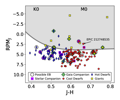
Figure 3: Reduced proper motion in $J$ band vs. $J-H$ color for all of the stars we observed and later classified as giants (yellow squares), hotter dwarfs (blue diamonds), or cool dwarfs (red circles). The gray line marks the dwarf/giant cut suggested by Collier Cameron et al. (2007); stars lying above this line (in the gray shaded region) are more likely to be giants while targets below the line are more likely to be dwarfs. For reference, we note the approximate $J-H$ colors of K0 and M0 stars. Note that some stars do not appear on this plot because they did not have proper motions reported in the EPIC.

The overarching goal of our project is to characterize planetary systems orbiting cool dwarfs observed by K2. Accordingly, we selected our targets from the set of planet candidate host stars. The majority of our targets were the putative hosts of candidate planets discovered by A. Vanderburg and the K2 California Consortium (K2C2), but we also consulted the public repository of K2 candidates provided by the NASA Exoplanet Archive (Akeson et al., 2013). We aimed to characterize all stars with proper motions and colors consistent with those of cool dwarfs (see Figure 3) as well as those for which the planet candidate discoverers estimated host star properties of $T_{\rm eff}\leq 5000$K and $\log g\geq 4.0$.

Over the 37 nights listed in Table 3, we observed 172 possible cool dwarfs that were identified as likely planet host stars. Many of these targets were selected from unpublished lists provided by A. Vanderburg (75 stars, 45%) or from the K2C2 candidate lists (93 stars, 56%) later published by Petigura et al. (2018), Livingston et al. (2018), Yu et al. (2018), and Crossfield et al. (2018). The majority of the targets appear on the K2 Candidates Table on the NASA Exoplanet Archive (109 stars, 65%). Those candidates were previously published by Montet et al. (2015, 7 stars), Adams et al. (2016, 5 stars), Barros et al. (2016, 24 stars), Crossfield et al. (2016, 37 stars), Libralato et al. (2016, 2 stars), Pope et al. (2016, 13 stars), Vanderburg et al. (2016, 56 stars), Schmitt et al. (2016, 2 stars), Mann et al. (2017a, 1 star), Rizzuto et al. (2017, 3 stars), Mayo et al. (2018, 22 stars), and Petigura et al. (2018, 19 stars). Note that there is substantial overlap across K2 candidate lists and that many stars appear on multiple lists.

One of the goals of our overall program is to determine the bulk and atmospheric composition of small planets. Accordingly, we tended to prioritize follow-up observations of candidate planets orbiting bright stars because brighter stars are more amenable to radial velocity mass measurement and subsequent atmospheric characterization. We also investigated candidate reliability by inspecting the K2 photometry of possible targets and consulting the ExoFOP-K2 follow-up website for notes from other observers. We avoided observing candidates already classified as eclipsing binaries and favored targets without nearby stellar companions. See the companion paper for a detailed discussion of the K2 Objects of Interest associated with each target star (Dressing, Vanderburg et al., in prep).

3 Observations

As in Dressing et al. (2017a), we conducted our observations using two medium resolution spectrographs: SpeX on the NASA Infrared Telescope Facility (IRTF) and TripleSpec on the Palomar 200”. Our SpeX observations were acquired during the 2016B - 2018A semesters as part of programs 2016B057, 2017A019, 2017B064, and 2018A073 (PI: Dressing). Our TripleSpec observations were obtained during 2016A - 2017B through programs P08, P03, P11, and P08 (PI: Dressing).

We provide additional details about the weather and targets observed during each run in Table 3. We reserved our faintest targets for the most pristine conditions and observed our brighter targets during poor weather. In all cases, we removed the telluric features from our science spectra by observing nearby A0V stars within one hour of our science observations (Vacca et al., 2003). We strove to find A0V stars at similar airmasses (difference $<0.1$ airmasses) and within $15^{\circ}$ of our target stars.

3.1 IRTF/SpeX

We conducted our SpeX observations in SXD mode using the $0\farcs 3\times 15\arcsec$ slit to acquire moderate resolution ($R\approx 2000$) spectra (Rayner et al., 2003, 2004). All of these observations were obtained after the SpeX upgrade in 2014 and therefore cover a broad wavelength range of 0.7 to 2.55 $\mu$m.

For each set of observations, we used an ABBA nod pattern with the default configuration of $7\farcs 5$ distance between the A and B positions. Each position was $3\farcs 75$ from the respective end of the slit. Unless a target was accompanied by a nearby companion, we aligned the slit to the parallactic angle to reduce systematics. For close binaries, we instead rotated the slit so that both stars could be observed simultaneously or so that the light from the nearby star would not contaminate the spectrum of the target star. We set integration times for each target based on the observing conditions and the stellar magnitude. We repeated the ABBA nod pattern as many times as needed so that the reduced spectra would have S/N $>100$ per resolution element. In order to minimize systematic effects due to hot pixels and alpha-particle decays from the ThF₄ anti-reflective coatings, we repeated the ABBA pattern at least three times regardless of the brightness of the star. We also limited individual exposure times to $<200$ s. The total exposure times varied from a few minutes to an hour depending on target brightness and observing conditions.

Throughout the night, we ran the standardized IRTF calibration sequence to acquire flats and wavelength calibration spectra. Both types of calibration data were taken using lamps; the flats were illuminated by an internal quartz lamp while the wavelength calibration spectra feature lines from an internal thorium-argon lamp. We usually acquired two sets of calibration spectra at the start and end of the night as well as at least one set per region of the sky. On nights when we observed the same part of the sky for many hours, we ran the calibration sequence multiple times per region so that each science spectrum could be reduced using calibration frames acquired within a few hours of the science spectrum.

3.2 Palomar/TripleSpec

We acquired our TripleSpec (TSPEC) observations using the fixed $1\arcsec\times 30\arcsec$ slit and therefore obtained simultaneous coverage between 1.0 and 2.4 $\mu$m at a spectral resolution of 2500-2700 (Herter et al., 2008). We mitigated contamination from bad pixels by conducting our observations using a four-position ABCD nod pattern rather than a two-position ABBA pattern more similar to our SpeX pattern. We adopted the same ABCD nod pattern as Muirhead et al. (2014) and Dressing et al. (2017a). As explained in Dressing et al. (2017a), we left the slit in the east-west orientation unless we were attempting to capture light from two stars simultaneously or avoid contamination from nearby stars. In order to calibrate our TripleSpec data, we obtained dome darks and dome flats at the start and end of each night.

4 Data Analysis &
Stellar Characterization

We reduced the NIR spectra of IRTF/SpeX targets using the publicly available Spextool pipeline (Cushing et al., 2004). For Palomar/TSPEC targets, we used a specialized version of Spextool adapted for using with TripleSpec data (available upon request from M. Cushing). We corrected all of our spectra for telluric contamination using the xtellcor package (Vacca et al., 2003), which is included in both versions of the Spextool pipeline. As in Dressing et al. (2017a), we used the Paschen $\delta$ line at 1.005 $\mu$m to create the convolution kernel needed to correct the Vega model spectrum for the instrumental profile and rotational broadening.

4.1 Initial Classification

After reducing the spectra, we determined the spectral types and luminosity classes of our target stars by comparing the reduced spectra to spectra of stars with known spectral types obtained from the IRTF Spectral Library (Rayner et al., 2009). We display representative SpeX and TSPEC spectra in Figures 1 and 2, respectively. We performed the comparison using the same interactive Python-based plotting interface described in Dressing et al. (2017a). Correcting for differences in stellar radial velocities and treating the $J$, $H$, and $K$ bandpasses individually, we computed the $\chi^{2}$ of a fit of each library spectrum to our data and recorded the best match for each bandpass. We then visually compared our spectra to the library spectra producing the lowest $\chi^{2}$ and selected the best match. We verified these final by-eye assignments by using parallaxes from the second Gaia data release (hereafter Gaia DR2; Gaia Collaboration et al., 2018b) to place our full sample on the Hertzsprung-Russell diagram (see Section 4.3).

As a further cross-check, we also measured the strength of three gravity-sensitive indices: K , Na I, and Ca II. All three indices were used by Mann et al. (2012) to investigate the luminosity classes of Kepler targets that were originally classified as M dwarfs. For our equivalent calculations, we adopted the band and continuum wavelength ranges shown in the final three rows of Table 2 of Mann et al. (2012).

The K I regions were defined in Mann et al. (2012), but the Na I and Ca II regions were chosen by Schiavon et al. (1997) and Cenarro et al. (2001), respectively.  As shown by Torres-Dodgen & Weaver (1993) and Schiavon et al. (1997), the Na I doublet (8172 - 8197Å) and K I (7669 - 7705Å) lines are significantly deeper in the spectra of dwarf stars than in the spectra of giant stars. In contrast, the Ca II triplet (8484-8662Å) is more pronounced in giant spectra than in dwarf spectra (e.g., Jones et al., 1984; Carter et al., 1986; Cenarro et al., 2001). All three of these indices are too blue to be measured in TSPEC data (wavelength range = 1.0 - 2.4 $\mu$m), but the agreement between the indices computed for our SpeX targets and our initial luminosity classifications suggests that our TSPEC targets are also correctly classified. Moreover, both our TSPEC targets and our SpeX targets have positions on the H-R diagram that are consistent with their assigned luminosity classes (see Section 4.3).

Although all of our targets were initially selected because they were believed to be likely cool dwarfs, we found that the sample was contaminated by giant stars and hotter dwarf stars. Overall, 86 (50%) of our targets were classified as cool dwarfs, 74 (43%) as hotter dwarfs (i.e., spectral types earlier than K5, effective temperatures above 4800K, or radii larger than $0.8{\rm\,R_{\odot}}$), and 12 (7%) as giant stars. We list the classifications in Table 4. We exclude the contaminating giants and hotter dwarfs from the detailed analyses in the rest of the paper, but the reduced spectra for all targets are posted on the ExoFOP-K2 website. For reference, Table 1 includes the relevant spectral indices for the seven SpeX targets classified as giant stars. The remaining five giants were observed with TSPEC and therefore lack coverage blueward of 1 $\mu$m. When available, Table 1 also includes proper motions and parallaxes from Gaia DR2.

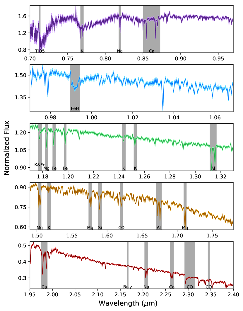
Figure 1: Reduced IRTF/SpeX spectrum (dark lines) of EPIC 206298289, which we classified as a cool dwarf with a spectral type of M1. The errors are depicted by the light shading around the spectrum.

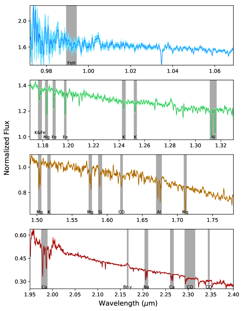
Figure 2: Reduced Palomar/TSPEC spectrum (dark lines) of EPIC 248433930, which we classified as a cool dwarf with a spectral type of M1. The errors are depicted by the light shading around the spectrum.

Compared to the initial stellar sample classified in Dressing et al. (2017a), this sample was slightly less contaminated by giant stars and slightly more contaminated by hotter stars. Of the 146 targets analyzed in Dressing et al. (2017a), 74 (51%) were classified as cool dwarfs, 49 (34%) as hotter dwarfs and 23 (16%) as giant stars. We attribute the reduced giant contamination in this paper to our stricter use of reduced proper motion cuts when selecting targets. The increase in the fraction of hotter dwarfs is likely due to our bias in prioritizing bright targets on nights with relatively poor weather conditions.

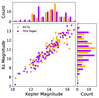
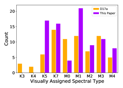
Figure 4: Distribution of magnitudes (top) and spectral types (bottom) for stars classified as cool dwarfs in this paper (purple) and in Dressing et al. (2017a, orange).

We display the magnitude and spectral type distribution for the 86 stars classified as cool dwarfs in Figure 4. Compared to the sample of 146 stars studied in Dressing et al. (2017a), this sample covers a slightly broader magnitude range ($7.2<Ks<13.6$ versus $7.9<Ks<13.1$) and has a brighter median magnitude ($Ks=10.7$ versus $Ks=11.3$). Although the Dressing et al. (2017a) cool dwarf sample included K3 and K4 dwarfs, this sample intentionally excludes stars earlier than K5. Relative to our earlier sample, this sample includes more K5 dwarfs, fewer M0 dwarfs, and more M1 dwarfs. However, our spectral type assignments are only accurate to $\pm 1$ spectral type and some of the stars classified as K7 or M1 may actually be M0 dwarfs.

4.2 Detailed Spectroscopic Classification

We initially estimated the physical properties of the cool dwarfs using the same procedures as in Dressing et al. (2017a) and display the results in Figure 5 and Table 5. Specifically, we used the publicly available, IDL packages tellrv and nirew (Newton et al., 2014, 2015) to implement the empirical relations established by Newton et al. (2015). These relations predict the stellar effective temperatures, radii, and luminosities of cool dwarfs from the equivalent widths of Al and Mg features measured in medium-resolution $H$-band spectra. The relations are valid for cool dwarfs with 3200 K$<T_{\rm eff}<$4800 K, $0.18{\rm\,R_{\odot}}<R_{\star}<0.8{\rm\,R_{\odot}}$, and $-2.5<\log L_{\star}/{\rm\,L_{\odot}}<-0.5$. As in Dressing et al. (2017a), we estimated the masses of the cool dwarfs by using the stellar effective temperature-mass relation from Mann et al. (2013b) to convert our temperature estimates into masses. We then calculated surface gravities from the estimated masses and radii.

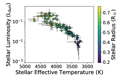
Figure 5: Parameters for the cool dwarf sample inferred from NIR spectroscopy. Left: Stellar luminosity vs. stellar effective temperature with points shaded according to revised stellar radii. Right: Radii and masses with points shaded according to revised stellar effective temperatures.

Our Palomar/TSPEC spectra were obtained at higher resolution than the IRTF/SpeX spectra used to calibrate the Newton et al. (2015) relations, so we downgraded the resolution of the Palomar/TSPEC spectra to that of the IRTF/SpeX data before measuring the equivalent widths. Ignoring the change in resolution could introduce a systematic $0.1{\emph{\AA}}$ difference in the measured equivalent widths (Newton et al., 2015); analyzing either downsampled Palomar/TSPEC data or unaltered IRTF/SpeX data yields consistent results (Dressing et al., 2017a).

In order to determine stellar metallicities, we implemented the relations defined in Mann et al. (2013a) for cool dwarfs with spectral types between K7 and M5. We first calculated metallicities using the $H$-band and $K$-band spectra separately and compared the results. Although the [Fe/H] and [M/H] estimates calculated from the $Ks$-band spectra were well-correlated, we found that the $H$-band [Fe/H] estimates displayed significant scatter relative to the $Ks$-band estimates. The $H$-band [M/H] estimates were consistent with the $Ks$-band [M/H] estimates, suggesting that the $H$-band [Fe/H] estimates are less reliable than the $Ks$-band estimates and more affected by telluric contamination. As shown in Table 3, many of our observations were obtained in partially cloudy conditions. To reduce weather-dependent systematics, we adopt the [Fe/H] and [M/H] estimates calculated from the $Ks$-band spectra instead of averaging the results from both bands. We display the resulting metallicities in Figure 6.

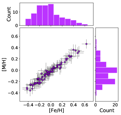
Figure 6: Estimated [Fe/H] and [M/H] for the cool dwarfs with spectral types of K7 or later.

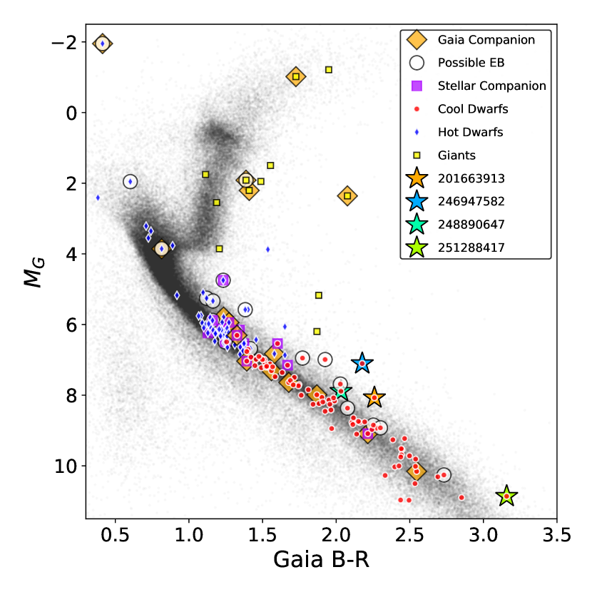
Figure 7: Color-magnitude diagram in $M_{G}$ vs. Gaia $B-R$ for all K2 targets with Gaia parallaxes (translucent black dots). The larger symbols mark K2OIs with Gaia parallaxes that we classify in this paper as giants (yellow squares), hotter dwarfs (blue diamonds), or cool dwarfs (red circles). Stars with nearby stellar companions are marked by purple squares and those suspected to be eclipsing binaries are surrounded by white circles.

4.3 Incorporating Gaia Distance Estimates

Our targets are moderately bright stars and might therefore be expected to have parallaxes reported in the second Gaia data release (Gaia Collaboration et al., 2018b). We checked for Gaia DR2 matches by using the Advanced ADQL tab of the Gaia Archive to create a list of all stars within $20"$ of the positions reported in the EPIC and compute their positions at the same reference epoch. We then selected all stars within $5"$ of our target stars and verified that the matches were genuine by comparing the proper motions and visual magnitudes ($G$ and $Kp$) of the target stars.

Of our 172 targets, 171 (99%) matched with stars in Gaia DR2 and 168 of those stars have reported parallaxes. We also identified 24 possible companion stars within $5"$ of 17 of our target stars. The star without a match in DR2 is the cool dwarf EPIC 204888276 and the stars with Gaia crossmatches but no reported parallaxes are EPIC 211783206 (hotter dwarf), EPIC 220187552 (cool dwarf), and EPIC 249483541 (cool dwarf). In total, 12 giant stars (100%), 73 hotter dwarfs (99%), and 83 cool dwarfs (97%) have parallaxes reported in Gaia DR2.

4.3.1 Possible Stellar Binaries

One cool dwarf (EPIC 210693462) appears to be a close binary because it has two matches within $1"$ of the stellar position reported by Huber et al. (2016) in the EPIC: Gaia DR2 44838019758175488 ($0\farcs 4$ away) and Gaia DR2 44838019756570112 ($0\farcs 3$ away). The two stars have similar parallaxes and proper motions. Based on the multiple Gaia matches and the presence of two stars in follow-up AO images obtained by D. Ciardi with Keck/NIRC2, we classify EPIC 210693462 as a binary and exclude it from the rest of the stellar characterization process in this paper. We performed a detailed characterization of the system in a separate paper (Feinstein et al., 2019).

Seventeen additional cool dwarfs have more distant candidate companions at angular separations of $1\farcs 5-5\farcs 0$. In order to assess whether any of these stars are physically associated with our target stars, we compared the relative proper motions and angular separations of each possible pair to the Lépine & Bongiorno (2007) criterion for likely co-movers. As shown in Table 2, the candidate stellar companions to EPIC 201650711 and EPIC 210693462 have parallaxes and proper motions similar to those of the primary star and are likely to be physically associated. In addition, EPIC 202071401 has one candidate companion that is likely to be physically associated (Gaia DR2 3378104379464943104) and one that is a likely interloper (Gaia DR2 3378104379464943232). The remaining candidate companions either have proper motions that are inconsistent with physical association (13 stars) or unknown proper motions (8 stars). As part of our check for possible stellar binaries, we consulted the ExoFOP-K2 website. Of the 172 stars in the full sample, 15 stars (9%; 7 cool dwarfs, 7 hotter dwarfs, & 1 giant star) were marked as possible eclipsing binaries, 9 stars (5%; 5 cool dwarfs & 4 hotter dwarfs) are in close proximity to stars revealed by follow-up imaging, and 5 stars (3%; 1 cool dwarf & 4 hotter dwarfs) are candidate EBs that also have candidate stellar companions. We include flags in Table 4 to identify possible stellar binaries.

The 5 cool dwarfs with candidate stellar companions are EPIC 206061524, EPIC 220187552, EPIC 220555384, EPIC 201119435, and EPIC 202071401. The candidate companion to EPIC 206061524 is roughly $0\farcs 5$ away from the target and detected in a Palomar/PHARO image obtained by D. Ciardi. EPIC 220187552 is a candidate eclipsing binary and is roughly $0\farcs 3$ away from a star that is approximately $0.68$ mag fainter at 832nm. Those estimates were determined from the WIYN speckle observations acquired by M. Everett but the companion was also detected in AO images obtained by D. Ciardi with Keck/NIRC2 and Palomar/PHARO. EPIC 220555384 also has an extremely close companion (separation $\approx 0.\farcs 2$) revealed by AO imaging at Lick, Gemini-N, and Palomar (images uploaded to ExoFOP by D. Ciardi) as well as speckle imaging at WIYN (image uploaded by M. Everett). The candidate companions to EPIC 201119435 and EPIC 202071401 were detected in Gaia DR2.

There are no posted follow-up images for most of the cool dwarfs with multiple companions in Gaia DR2, but the candidate companions to EPIC 201119435 and EPIC 202071401 are visible in AO images obtained by D. Ciardi with Gemini-N/NIRI, Palomar/PHARO, and Keck/NIRC2. The companion to EPIC 202071401 was not detected in the WIYN speckle image obtained by M. Everett, but the star may have been outside the $2\farcs 8\times 2\farcs 8$ field-of-view.

4.3.2 Absolute Magnitudes

For all stars except EPIC 210693462 (the close binary), we calculated absolute $Ks$ magnitudes from the distance estimates determined by Bailer-Jones et al. (2018). For our full target sample, the parallaxes reported in Gaia DR2 range from 0.07 mas to 35.8 mas (Gaia Collaboration et al., 2018b), which corresponds to a distance range of 28–8546 pc (Bailer-Jones et al., 2018). The 86 cool dwarfs have parallaxes of 1.7–35.8 mas and estimated distances of 28–589 pc with a median distance of 127 pc. Our distance estimates are drawn from Bailer-Jones et al. (2018) and carry a Bayesian transformation of the parallax probability distribution function into a distance probability distribution function, using Bayesian priors selected for each star.

Next, we used the absolute magnitudes to place our targets on the color-magnitude diagram shown in Figure 7 and confirm our stellar classifications. For the cool dwarfs with parallaxes in Gaia DR2, we then used the photometric relations described in Sections 4.3.3–4.3.6 to estimate stellar radii, masses, and effective temperatures. We list the resulting parameters in Table 6.

In Figure 7, we indicate which stars have been flagged as possible EBs on the ExoFOP-K2 website and which stars have possible stellar companions revealed by ground-based follow-up images or Gaia astrometry. The three cool dwarfs that are flagged as possible EBs and are clearly above the main sequence in Figure 7 are EPIC 248527514, EPIC 205996447, and EPIC 212009427. Note that EPIC 220187552 (also flagged as suspected EB) does not appear on Figure 7 because Gaia DR2 does not include a parallax for this star.

The cool dwarfs that fall above the main sequence and are not flagged as likely EBs are EPIC 201663913 (1.2 magnitudes brighter than stars with similar $B_{p}-R_{p}$ colors), EPIC 246947582 (1.8 magnitudes brighter), EPIC 248890647 (0.6 magnitude brighter), and EPIC 251288417 (1.1 magnitude brighter). There are no follow-up images of EPIC 201663913, EPIC 248890647, or EPIC 251288417 on the ExoFOP-K2 website, but EPIC 246947582 ($G=7.10$, $B-R=2.18$) was observed by D. Ciardi using Keck/NIRC2 with a Br-$\gamma$ filter. Ciardi did not detect any nearby companions down to a limit of $\Delta M=6$ at $0\farcs 2$ and $\Delta M=7$ at $0\farcs 7$. EPIC 201663913 is 0.83 magnitudes brighter.

4.3.3 Stellar Luminosities

With the exception of EPIC 210693462 (the close binary), we determined photometric luminosity estimates for all cool dwarfs with adequate photometry. Following Mann et al. (2017b), we began by consulting the Carlsberg Meridian Catalogue (Muiños & Evans, 2014) to find $r$-band magnitudes for each star. We then inferred $L_{\star}$ from the 2MASS $J$ magnitudes reported in the EPIC (Huber et al., 2016; Skrutskie et al., 2006), $J$-band bolometric corrections determined from $r-J$ colors using the relations established by Mann et al. (2015), and the estimated stellar distances reported by Bailer-Jones et al. (2018).

We compare these photometric luminosity estimates to our spectroscopic estimates in the top left panel of Figure 8. We find that the spectroscopic and photometric estimates agree well for single stars with spectroscopic luminosity estimates $L_{\star,spec}<0.025{\rm\,L_{\odot}}$ but that there is a systematic difference between the spectroscopic and photometric estimates for brighter stars. The photometric estimates are brighter than the spectroscopic estimates for stars with intermediate brightness ($0.025{\rm\,L_{\odot}}<L_{\star,spec}<0.13{\rm\,L_{\odot}}$) and fainter than the spectroscopic estimates for the brightest stars ($L_{\star,spec}>0.13{\rm\,L_{\odot}}$).

Gaia DR2 includes luminosity estimates for 50 of the cool dwarfs in our sample. Andrae et al. (2018) determined stellar parameters by using the Final Luminosity Age and Mass Estimator (FLAME) and Priam algorithms to infer stellar luminosities, radii, and effective temperatures from Gaia parallaxes and three-band photometry ($G$, $G_{\rm BP}$, $G_{\rm RP}$). Both modules are part of the larger Gaia astrophysical parameter inference system (Apsis, Bailer-Jones et al., 2013).

As shown in the top middle panel of Figure 8, the Gaia luminosity estimates follow the same trend as the spectroscopic luminosities we estimated from the Newton et al. (2015) relations in Section 4.2. However, the Newton estimates are slightly lower for fainter cool dwarfs and higher for brighter cool dwarfs. Note that Andrae et al. (2018) do not report luminosities or radii for stars smaller than $R_{\star}=0.5{\rm\,R_{\odot}}$. For field-age cool dwarfs, this boundary roughly corresponds to $M_{\star}=0.5{\rm\,M_{\odot}}$, $T_{\rm eff}=3660$ K, and spectral types of M1 – M2.

There are several stars with precise Gaia luminosity estimates that are significantly higher than their spectroscopic luminosity estimates. Many of these stars have already been identified as stellar binaries, some of which are eclipsing and generated transit-like signals in the K2 photometry. Figure 8 demonstrates that combining spectroscopic characterization with photometric characterization is an efficient way to identify close binaries even in the absence of high-resolution follow-up imaging: stars in unresolved binaries appear overly luminous to photometric surveys but stellar spectroscopy enables independent estimates of stellar luminosities. As would be expected for unresolved binaries, the Gaia luminosities calculated for the stars identified as possible EBs are larger than our spectroscopic estimates.

Neglecting the five stars with nearby companions (four of which have Gaia luminosity estimates) and the seven stars flagged as likely eclipsing binaries (five of which have Gaia luminosity estimates), the median difference between the luminosity estimates is $\Delta L_{\star}=L_{\star,spec}-L_{\star,Gaia}=-0.003{\rm\,L_{\odot}}$ and the standard deviation of the difference is $\Delta L_{\star}$ is $0.043{\rm\,L_{\odot}}$. However, while the median difference is small, Figure 8 reveals that the difference between the Gaia luminosity estimates and the spectroscopic luminosity estimates is luminosity-dependent. The Gaia estimates are lower than our spectroscopic estimates for stars with $L_{\star,Gaia}<0.12{\rm\,L_{\odot}}$ and higher for brighter stars. The differences are roughly $0.02{\rm\,L_{\odot}}$ at the low luminosity end ($L_{\star,Gaia}<0.12{\rm\,L_{\odot}}$) and $0.03{\rm\,L_{\odot}}$ at the high luminosity end ($L_{\star,Gaia}>0.12{\rm\,L_{\odot}}$).

The top right panel of Figure 8 reveals that our photometric luminosity estimates are consistent with the Gaia luminosity estimates. All of the stars are tightly near the one-to-one relation but our photometric estimates are slightly lower than the Gaia luminosity estimates. The median difference between the luminosity estimates is $\Delta L_{\star}=L_{\star,phot}-L_{\star,Gaia}=-0.005{\rm\,L_{\odot}}$ and the standard deviation of the difference is $\Delta L_{\star}$ is $0.010{\rm\,L_{\odot}}$. For the closest stars ($d<75$ pc), the Gaia estimates are roughly $0.01{\rm\,L_{\odot}}$ larger than the photometric estimates. This difference decreases with increasing distance for distances between 29 pc and 130 pc. For intermediate distances of 130 – 200 pc, the Gaia estimates are roughly $0.003{\rm\,L_{\odot}}$ smaller than the photometric estimates. Finally, for distances of 200 – 500 pc, the Gaia estimates are roughly $0.008{\rm\,L_{\odot}}$ larger than the photometric estimates.

As discussed in Section 4.4, for our final stellar catalog, we adopt the photometric luminosities when possible and the spectroscopic luminosities for stars without parallaxes in Gaia DR2. We favor the photometric luminosities over the spectroscopic luminosities because the relations from Newton et al. (2015) that we use to calculate spectroscopic luminosities were calibrated using a sample of only 25 stars with interferometrically-determined radii while the photometric luminosities are derived directly from photometry, precisely determined parallaxes from Gaia DR2 (Gaia Collaboration et al., 2018b), and established bolometric corrections (Mann et al., 2015).

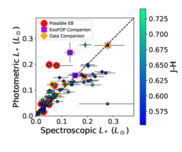
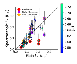
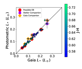
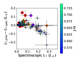
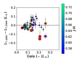
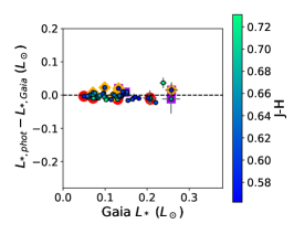
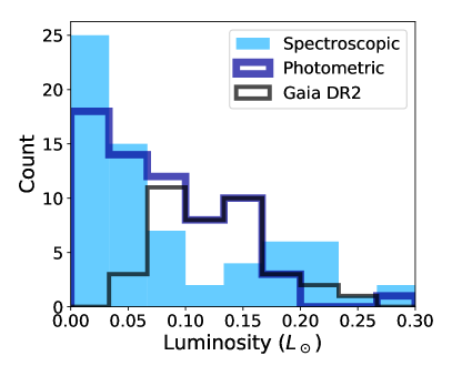
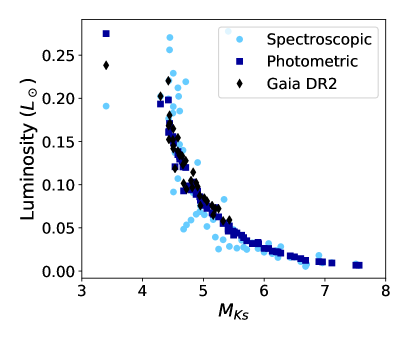
Figure 8: Comparison of stellar luminosities and radii estimated from spectroscopy and photometry. We denote the values estimated in this paper as “spectroscopic” if they are primarily determined from our NIR spectra or “photometric” if they are determined from the combination of broadband photometry and Gaia parallaxes. We also compare our estimates to those determined by the Gaia team; those values are also photometric, but they are marked here as “Gaia” to avoid confusion. The points are color-coded by $J-H$ color. In panels displaying individual stars, we indicate possible EBs by wrapping the points with red circles. We also use orange diamonds to mark stars with companions in Gaia DR2 and purple squares to flag stars with nearby stellar companions detected in AO or speckle images. The black dashed lines mark a 1:1 correlation. Top Left: Photometric luminosity estimates versus spectroscopic luminosity estimates. Top Center: Spectroscopic luminosity estimates versus luminosity estimates from Gaia DR2. Top Right: Photometric luminosity estimates versus Gaia luminosity estimates. Middle Left: Difference between photometric and spectroscopic luminosity estimates versus spectroscopic estimates. Middle Center: Difference between spectroscopic luminosity estimates and those from Gaia DR2 versus Gaia DR2 estimates. Middle Right: Difference between photometric luminosity estimates and those from Gaia DR2 versus Gaia DR2 estimates.Bottom Left: distribution of luminosities for stars in the cool dwarf sample that have not been classified as likely EBs and do not have stellar companions (i.e., “single cool dwarfs”). Bottom Right: Luminosity versus absolute $Ks$ magnitude for single cool dwarfs. The extremely bright star is EPIC 246947582; see Section 4.3.2.

4.3.4 Stellar Radii

We estimated stellar radii using the empirical equations from Table 1 of Mann et al. (2015, 2016). For the 66 cool dwarfs with Gaia parallaxes and spectral types of K7 or later, we calculated stellar radii by employing the $R_{\star}-M_{Ks}-$[Fe/H] relation given in their Equation 5; for the metallicity-dependent term, we used the [Fe/H] values calculated in Section 4.2. For the 17 K5 dwarfs with Gaia parallaxes, we dropped the metallicity dependence because the stars were too hot for our selected metallicity relation and used the simpler $R_{\star}-M_{Ks}$ relation described by their Equation 4. The systematic errors on the $R_{\star}-M_{Ks}-$[Fe/H] and $R_{\star}-M_{Ks}$ relation are 2.70% and 2.89%, respectively (Mann et al., 2015, 2016). Our quoted errors on the stellar radii incorporate both these systematic errors and the uncertainties on $M_{Ks}$ and [Fe/H].

The relations are valid for K7 – M7 dwarfs with $4.6<M_{Ks}<9.8$ and $-0.6<{\rm[Fe/H]}<0.5$. Most of the cool dwarfs with parallaxes fall within those limits (59 stars; 69%), but one is too metal-rich ([Fe/H] = 0.63) and 23 are too bright. We do not report photometric radius estimates for the six brightest stars, but we used the equations from Mann et al. (2015) to extrapolate the relations slightly to cover $4.3<M_{Ks}<9.8$ and $-0.6<{\rm[Fe/H]}<0.65$ so that we can estimate radii for 18 stars that are only slightly outside the calibration range. We have included a flag in Table 6 to indicate which stars have absolute magnitudes or metallicities outside the range recommended by Mann et al. (2015).

As shown in the upper two left panels of Figure 9, the photometric radius estimates agree well with the spectroscopic estimates found in Section 4.2. Considering only the 65 stars that appear to be single and have radius estimates from both methods, the median difference $\Delta R_{\star}=R_{\star,phot}-R_{\star,spec}=0.02{\rm\,R_{\odot}}$ (3%) and the standard deviation in the distribution of $\Delta R_{\star}$ is $\sigma_{\Delta R_{\star}}=0.05{\rm\,R_{\odot}}$. Mann et al. (2017a) previously noted that the spectroscopic radii estimated by Newton et al. (2015) are consistent with the photometric radii estimated by their $R_{\star}-M_{Ks}-$[Fe/H] relation (Mann et al., 2015), so this result is not surprising.

The top two center panels of Figure 9 contrast our spectroscopic radius estimates to those estimated by the Gaia team using Apsis-FLAME (Bailer-Jones et al., 2013; Andrae et al., 2018). Only 50 cool dwarfs have radius estimates in DR2 and all of those stars are at least $0.5{\rm\,R_{\odot}}$ because Andrae et al. (2018) do not report luminosity or radius estimates for smaller stars. The median difference for the 38 supposedly single stars is $\Delta R_{\star}=R_{\star,spec}-R_{\star,Gaia}=-0.01{\rm\,R_{\odot}}$ (-2%) and the standard deviation of the differences is $\sigma_{\Delta R_{\star}}=0.1{\rm\,R_{\odot}}$. Although these differences are small, there is a noticeable trend between the radius discrepancy and the estimated radius. Our spectroscopic estimates tend to be larger than the value estimated by the Gaia team for stars with $R_{\star,Gaia}>0.6{\rm\,R_{\odot}}$ and lower than the Gaia estimates for stars with $R_{\star,Gaia}>0.6{\rm\,R_{\odot}}$ .

Predictably, the possible eclipsing binaries have larger radius estimates from Gaia than from spectroscopy because the added light from a companion star causes them to appear overluminous in Gaia. Two purportedly single stars also have large radius discrepancies: the M1 dwarf EPIC 201663913 has a Gaia radius estimate of $R_{\star,Gaia}=0.84{\rm\,R_{\odot}}$ and a spectroscopic estimate of $R_{\star,spec}=0.53{\rm\,R_{\odot}}$ while the K7 dwarf EPIC 246947582 has $R_{\star,Gaia}=1.25{\rm\,R_{\odot}}$ and $R_{\star,spec}=0.61{\rm\,R_{\odot}}$. These stars were assigned radii of $0.403{\rm\,R_{\odot}}$ and $0.428{\rm\,R_{\odot}}$, respectively, in the Ecliptic Plane Input Catalog (Huber et al., 2016). As noted in Section 4.3.2, there are no follow-up observations of EPIC 201663913 posted to the ExoFOP website, but D. Ciardi acquired a high-resolution image of EPIC 246947582 using NIRC2 on Keck 2 and did not detect any companions.

Finally, the upper two right panels of Figure 9 compare our photometric radius estimates to the Gaia radius estimates (Bailer-Jones et al., 2013; Andrae et al., 2018). Six of the 50 stars with Gaia radius estimates are too bright for the Mann et al. (2015, 2016) relations. The remaining 44 cool dwarfs have both Gaia radius estimates and photometric radius estimates from this paper and 36 are supposedly single. The median difference for those 36 stars is $\Delta R_{\star}=R_{\star,phot}-R_{\star,Gaia}=0.02{\rm\,R_{\odot}}$ (3%) and the standard deviation of the differences is $\sigma_{\Delta R_{\star}}=0.06{\rm\,R_{\odot}}$. As in the center panels, we note that the radius difference is correlated with the radius estimated by the Gaia team. Specifically, our photometric estimates tend to be larger than the Gaia estimates for the 18 stars with $R_{\star,Gaia}>0.64{\rm\,R_{\odot}}$. For the 18 larger stars, there is still scatter in the relation but the median difference is closer to zero ($-0.013{\rm\,R_{\odot}}$ versus $0.049{\rm\,R_{\odot}}$ for smaller stars).

In our stellar catalog, we select the photometric radii when possible and default to spectroscopic radii for the nine stars without photometric estimates. Three of the stars with spectroscopic radius estimates lack parallaxes in Gaia DR2 and the remaining six are too bright for the empirical relations from Mann et al. (2015, 2016). The spectroscopic sample contains a high fraction of likely eclipsing binaries (three stars) and stars with candidate stellar companions (three stars).

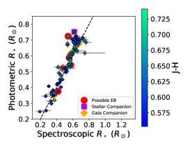
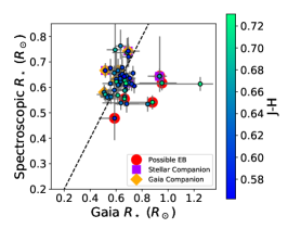
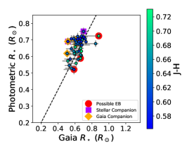
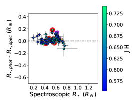
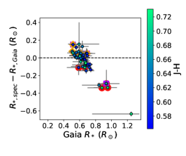
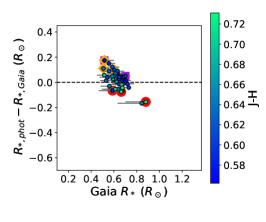
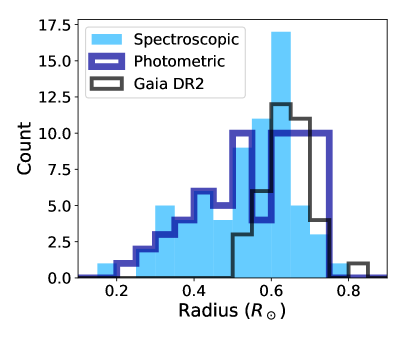
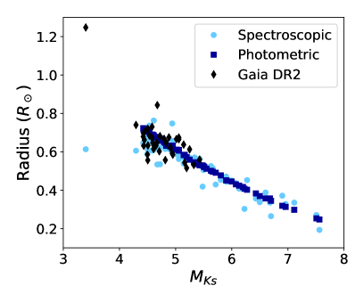
Figure 9: Same as Figure 8, but for stellar radii. The Gaia sample is restricted to stars larger than $0.5{\rm\,R_{\odot}}$.

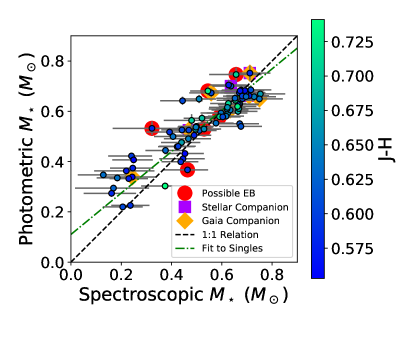
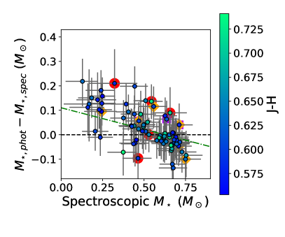
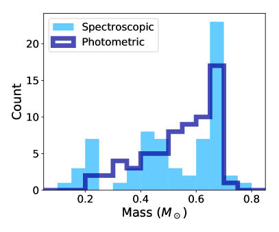
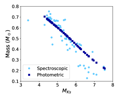
Figure 10: Same as Figure 8, but for stellar masses. The Gaia panels are missing because Gaia DR2 does not include estimates of stellar mass. In the top row,

the green dotted-dash lines are a linear fit to all of the purportedly single stars and the black dashed lines mark a 1:1 correlation.

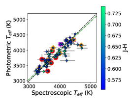
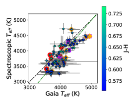
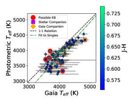
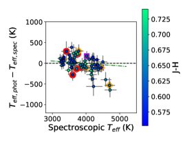
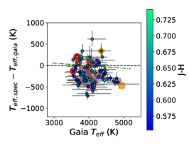
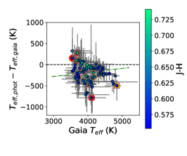
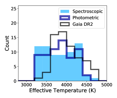
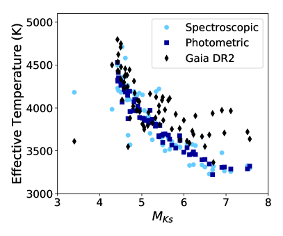
Figure 11: Same as Figure 8, but for stellar effective temperatures.

4.3.5 Stellar Masses

We estimated masses by employing the $M_{\star}-M_{Ks}$ empirical relation from Mann et al. (2019), which was constructed by using parallaxes, imaging, and astrometry to constrain the orbits and masses of 62 nearby stellar binaries. Mann et al. (2019) present six different $M_{\star}-M_{Ks}$ relations ranging in complexity from fourth to sixth order in $M_{Ks}$. Half of the relations incorporate a metallicity-dependent term while the remaining three are independent of metallicity. Following the advice in the paper, we used the fifth order fit and did not incorporate metallicity because the current sample of cool dwarfs with precisely determined masses is too small to warrant the addition of a metallicity-dependent term (Mann et al., 2019).

The new $M_{\star}-M_{Ks}$ relation from Mann et al. (2019) agrees well (within 5%) with the earlier Delfosse et al. (2000) relation for stars with masses $0.15{\rm\,M_{\odot}}<M_{\star}<0.5{\rm\,M_{\odot}}$ and predicts masses that are roughly 10% higher for more massive stars where the Delfosse et al. (2000) sample was sparse. For stellar masses of $0.09{\rm\,M_{\odot}}-0.25{\rm\,M_{\odot}}$, the $M_{\star}-M_{Ks}$relation from Mann et al. (2019) also agrees well with the relation from Benedict et al. (2016), but for stars with $M_{\star}>0.3{\rm\,M_{\odot}}$, Mann et al. (2019) find masses that are 10% lower than those predicted by Benedict et al. (2016) relation. Mann et al. (2019) attribute this discrepancy to the inclusion of eclipsing binaries and stars with poor $M_{Ks}$ estimates in the stellar sample used by (Benedict et al., 2016). For this paper, we opted to use the relation from Mann et al. (2019) because it is the most recent $M_{\star}-M_{Ks}$ relation available in the literature for cool dwarfs and based upon a well-vetted sample of stars with precisely and accurately determined properties.

The $M_{\star}-M_{Ks}$ relation from Mann et al. (2019) is valid for stars with activity levels and metallicities similar to those of nearby stellar neighbors and absolute magnitudes of $4.0<M_{Ks}<11.0$, which corresponds to masses of $0.075{\rm\,M_{\odot}}<M_{\star}<0.75{\rm\,M_{\odot}}$. Our cool dwarf sample includes 80 stars within this absolute magnitude range, three brighter stars with $3.4<M_{Ks}<3.9$, and three stars without parallaxes in Gaia DR2. We do not estimate photometric stellar masses for the three brighter stars. These targets are EPIC 220555384 (which has a nearby stellar companion reported on ExoFOP), EPIC 205947214 (which is flagged as a likely EB on ExoFOP), and EPIC 246947582.

The top left panel of Figure 10 demonstrates that the photometric mass estimates are systematically offset from the spectroscopic mass estimates. Ignoring the stars with nearby companions or those flagged as likely eclipsing binaries, the median mass difference for the 66 purportedly single stars is $\Delta M_{\star}=M_{\star,phot}-M_{\star,spec}=0.002{\rm\,M_{\odot}}$ (0.2%) with a standard deviation of $0.08{\rm\,M_{\odot}}$. Our stellar sample is relatively small, but the offset between the spectroscopic and photometric estimates seems to be larger at the low-mass end. The realization that the discrepancy is largest for the lowest stellar masses is particularly problematic because even a small difference can be a large fraction of the total stellar mass for the coolest stars.

Subdividing the sample by spectroscopic mass estimate, $\Delta M_{\star}=0.11{\rm\,M_{\odot}}$ (34%) for the 11 stars with $M_{\star,phot}<0.4{\rm\,M_{\odot}}$, $\Delta M_{\star}=0.03{\rm\,M_{\odot}}$ (6%) for the 27 stars with $0.4\leq{\rm\,M_{\odot}}<M_{\star}<0.6{\rm\,M_{\odot}}$, and $\Delta M_{\star}=-0.02{\rm\,M_{\odot}}$ (-3%) for the 28 more massive stars. Fitting a line to the apparently single stars and accounting for the errors in both $M_{\star,spec}$ and $M_{\star,phot}$, we find that $M_{\star,phot}$ can be estimated from $M_{\star,spec}$ using a linear fit with slope $m=0.82\pm 0.05$ and y-intercept $b=0.11\pm 0.03$.

For our final stellar catalog, we adopt the photometric mass estimates because those are calculated directly from the absolute magnitudes of our target stars rather than indirectly by applying the older $T_{\rm eff}-M_{\star}$ relation derived by Mann et al. (2013b) to our spectroscopic temperature estimates. The new $M_{\star}-M_{Ks}$ relation from Mann et al. (2019) is based on a larger and more comprehensively scrutinized sample of cool dwarfs than the earlier $T_{\rm eff}-M_{\star}$ relation. For the two stars without parallaxes reported in Gaia DR2, we estimate masses by using the mass-radius relation found for the photometric sample to predict the masses of stars with radii equal to our spectroscopic radius estimates. Adopting this strategy accounts for the discrepancy between photometric and spectroscopic masses (see Figure 10).

4.3.6 Stellar Effective Temperatures

We determined photometric temperature estimates for all cool dwarfs with adequate photometry using the same procedure as Mann et al. (2017b). We began by estimating stellar luminosities as described in Section 4.3.3. We then combined our luminosity estimates with the photometric radii estimated in Section 4.3.4 and calculated stellar effective temperatures from the Stefan-Boltzmann relation.

In the top left two panels of Figure 11, we compare these photometric temperature estimates to the spectroscopic estimates determined in Section 4.2. Overall, the photometric estimates agree well with the spectroscopic estimates. For the 64 presumedly single stars with both spectroscopic and photometric estimates, the median difference $\Delta T_{\rm eff}=T_{{\rm eff},phot}-T_{{\rm eff},spec}=-3$K and the standard deviation of the differences is $\sigma_{\Delta T_{\rm eff}}=172$K.

Mann et al. (2017b) conducted a similar comparison of spectroscopic and photometric temperature estimates. They found that the temperatures estimated via the Stefan-Boltzmann relation were consistent with the spectroscopic estimates determined by Newton et al. (2015), but that the Newton et al. (2015) estimates displayed more scatter. As shown in the bottom right panel of Figure 11, our photometric temperature estimates also exhibit a slightly tighter relation with $M_{Ks}$ than our spectroscopic estimates.

In the top center two panels of Figure 11, we investigate the similarity between our spectroscopic temperature estimates and those estimated by the Gaia team using Apsis-Priam (Bailer-Jones et al., 2013; Andrae et al., 2018). At all spectroscopic temperatures, our estimates tend to be lower than those estimated by the Gaia team. Specifically, we find that the median difference $\Delta T_{\rm eff}=T_{{\rm eff},Gaia}-T_{{\rm eff},spec}=198$K (5%) for the 68 supposedly single stars with temperature estimates in Gaia DR2. The standard deviation of the difference distribution is $\sigma_{\Delta T_{\rm eff}}=266K$.

The top right two panels of Figure 11 compare our photometric temperature estimates to those estimated by the Gaia team using Apsis-Priam (Bailer-Jones et al., 2013; Andrae et al., 2018). In the Apsis-Priam framework, $T{\rm eff}$ is estimated from observed brightness of the target star in the three Gaia photometric bands assuming zero extinction. The estimates are determined using a machine-learning algorithm training on a set of stars with known temperatures and low extinctions. The Gaia temperature estimates are noticeably larger than our own photometric temperature estimates. For the 64 stars with temperature estimates from both methods and no evidence of stellar companions, the median difference $\Delta T_{\rm eff}=T_{{\rm eff},phot}-T_{{\rm eff},Gaia}=-191$K (-5%) and the standard deviation of the differences is $\sigma_{\Delta T_{\rm eff}}=200$K.

Andrae et al. (2018) noted a similar offset between their temperature estimates and literature values for low-mass dwarfs ($\log g\gtrsim 4.8$). They proposed that the discrepancy might be due to temperature errors induced by the presence of strong molecular absorption in the broad-band integrated photometry of cool dwarfs or to the possible tendency of Apsis-Priam to overestimate the extinction and temperatures of cool dwarfs. Apsis-Priam assigns stellar parameters by using a machine learning algorithm trained on observations of real stars, most of which are much farther away than these cool dwarfs and therefore have higher extinction. Accordingly, we provide the Gaia $T_{\rm eff}$ estimates for comparison purposes only; we do not recommend using those values for cool dwarfs.

When compiling our final cool dwarf catalog, we select the photometric temperature estimates for all stars with reported parallaxes. For stars without parallaxes, we instead adopt the spectroscopic estimates. As previously noted by Mann et al. (2017b), our spectroscopic and photometric temperature estimates are in agreement but the spectroscopic estimates display more scatter.

4.4 Overall Comparison of Spectroscopic & Photometric Estimates

In Figure 12, we compare the stellar radii and effective temperatures resulting from the spectroscopic analysis in Section 4.2 and the photometric analysis in Section 4.3. For clarity, we exclude the five stars identified as possible eclipsing binaries (EBs) and the seven stars with detected nearby companions in Gaia DR2 or follow-up images. There are therefore 65 stars included in both the $R_{\star}-M_{\star}$ and the $R_{\star}-T_{\rm eff}$ panels.

Our photometric radius and mass estimates are both primarily determined by $M_{Ks}$, leading the photometric estimates to follow a tight trend on the left panel of Figure 12. In contrast, the spectroscopic estimates are more broadly dispersed. At the more massive end of the cool dwarf sample ($M_{\star}>0.67{\rm\,M_{\odot}}$), there is cluster of stars for which the spectroscopic radius estimates are roughly 10% lower that the photometric estimates, indicating that the spectroscopic relations may systematically underestimate the radii of the most massive cool dwarfs.

The difference between the spectroscopic and photometric estimates is less stark in the $R_{\star}-T_{\rm eff}$ plot displayed in the right panel of Figure 12. Although our photometric estimates incorporate the spectroscopic [Fe/H] constraints when possible, the difference between [Fe/H]-dependent photometric estimates and [Fe/H]-free photometric estimates is much smaller than the overall difference between the photometric and spectrosopic estimates. The [Fe/H]-dependent radius estimates fall nearly on top of the [Fe/H]-free radius estimates: the median $\Delta R_{\star}=R_{\star,{\rm[Fe/H]}}-R_{\star,{no\rm[Fe/H]}}=-0.002{\rm\,R_{\odot}}$ (-0.4%) with a standard deviation of $0.005{\rm\,R_{\odot}}$. (This quoted difference was calculating using the 52 stars with spectral types of K5 or later; the [Fe/H]-based relations are not valid for K7 dwarfs.)

Assuming that the [Fe/H]-dependent photometric estimates are the “true” values, the $M_{Ks}$-based photometric relations employed in Sections 4.3.5–4.3.6 yield remarkably accurate and precise stellar properties even in the absence of [Fe/H] constraints. Accordingly, we are now using the combination of Gaia DR2 data (Gaia Collaboration et al., 2018b) and archival photometry from the KIC (Brown et al., 2011) and EPIC (Huber et al., 2016) to produce catalogs of updated properties for all K2 and Kepler cool dwarfs (Schwab Abrahams, Dressing et al., in prep).

For the remainder of the paper, we restrict the discussion to the 75 stars that have not been classified as likely eclipsing binaries and do not have candidate stellar companions within $1"$. Nearly all of these stars (97%) have parallaxes reported in Gaia DR2. For the 73 stars with Gaia parallaxes, we adopt the photometric estimates as our preferred values for each star. These estimates incorporate our spectroscopic estimates of [Fe/H] for the 56 stars with Gaia parallaxes and spectral types of K7 or later and are agnostic to [Fe/H] for the 17 K5 dwarfs with Gaia parallaxes. For the remaining two stars without Gaia parallaxes, we resort to our spectroscopic estimates, but replace the spectroscopic masses by those found by interpolating the mass - radius relation found for the photometric sample because of the discrepancy between photometric and spectroscopic masses (see Figure 10 and Section 4.3.5). Even though we adopt photometric estimates when possible, our spectroscopic characterization was important for determining spectral types, estimating stellar metallicities, and identifying close stellar binaries.

Accounting for the validity ranges of the various photometric relations, our sample includes 70 cool dwarfs with photometric radius and mass estimates and five with spectroscopic radius estimates based on the Newton et al. (2014, 2015) relations and masses estimated by placing the spectroscopic radii on the photometric mass-radius relation. We adopt the photometric luminosities for 43 cool dwarfs and report spectroscopic estimates based on Newton et al. (2014, 2015) for the remaining 32 cool dwarfs. All stars have photometric temperature estimates based on the relations from Mann et al. (2015).

We list the adopted parameters for all 75 cool dwarfs presumed to be single in Table 7 and display the resulting distribution of stellar radii and effective temperatures in Figure 13. The radii range from $0.24{\rm\,R_{\odot}}$ to $0.74{\rm\,R_{\odot}}$ with a median value of $0.58{\rm\,R_{\odot}}$ and the stellar effective temperatures extend from 3178K to 4531K with a median value of 3851K. Compared to the sample of cool dwarfs we characterized in Dressing et al. (2017a), this sample is shifted toward higher radii and cooler stellar effective temperatures. The offset is partially due to our use of spectroscopic estimates in Dressing et al. (2017a) and predominantly photometric estimates in this paper as well as sample selection effects influencing both the original K2 target lists and the sample of stars for which we obtained follow-up observations.

In summary, we reached the following conclusions from comparing the spectroscopic and photometric stellar parameters calculated in this paper to those reported in Gaia DR2:

• Our photometric estimates of stellar luminosity are consistent with those reported in Gaia DR2 (Gaia Collaboration et al., 2018b).

• Relative to our photometric estimates, our spectroscopic luminosities are roughly $0.03{\rm\,L_{\odot}}$ brighter for the brightest stars ($L_{\star,spec}>0.13{\rm\,L_{\odot}}$).

• Our photometric and spectroscopic estimates of stellar radius agree well. Across our full cool dwarf sample, the median radius difference is only $0.02{\rm\,R_{\odot}}$, with the photometric estimates slightly larger than the spectroscopic estimates.

• The stellar radii reported in Gaia DR2 are systematically offset from our spectroscopic and photometric estimates. Compared to our photometric estimates, the Gaia estimates are roughly $0.04{\rm\,R_{\odot}}$ smaller for stars with $R_{\star,phot}>0.67{\rm\,R_{\odot}}$.

• Our photometric and spectroscopic mass estimates are correlated, but our spectroscopic estimates are smaller than our photometric estimates for the least massive stars and larger than our photometric estimates for the most massive stars. The discrepancy is roughly $M_{\star,phot}-M_{\star,spec}=0.11{\rm\,M_{\odot}}$ for stars with $M_{\star,phot}<0.4{\rm\,M_{\odot}}$ and $-0.02{\rm\,M_{\odot}}$ for stars with $M_{\star,phot}>0.6{\rm\,M_{\odot}}$.

• Our photometric and spectroscopic temperature estimates agree well (median difference of $T_{{\rm eff},phot}-T_{{\rm eff},spec}=-3$K), but the temperatures reported in Gaia DR2 are roughly 200K higher than our estimates.

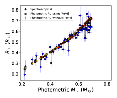
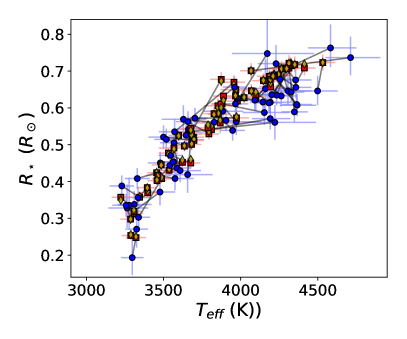
Figure 12: Comparison of stellar parameters estimated from spectroscopy and photometry. Left: Radius versus mass for estimates based on spectroscopy (blue circles), photometry incorporating knowledge of [Fe/H] (red squares), and photometry without [Fe/H] constraints (yellow diamonds). The gray lines connect the spectroscopic and [Fe/H]-free photometric estimates for each star to the [Fe/H]-based photometric estimates. Right: Radius versus stellar effective temperature.

5 Discussion

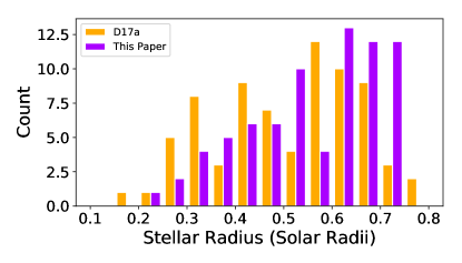
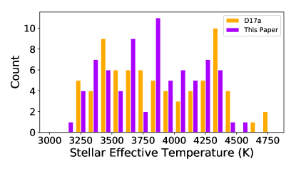
Figure 13: Distribution of radii (top) and effective temperatures (bottom) for the cool dwarfs analyzed in this paper (purple) compared to those previously characterized in Dressing et al. (2017a, orange).

As mentioned in Section 2, we observed these stars because they were initially identified as candidate cool dwarfs. In Figures 14 and 15, we compare our revised stellar parameters to earlier estimates from the Ecliptic Plane Input Catalog (EPIC, Huber et al., 2016) and previous studies. Several of the earlier planet catalogs did not estimate host star parameters (Barros et al., 2016; Pope et al., 2016; Schmitt et al., 2016; Rizzuto et al., 2017). The top and left panels of Figure 14 contrast our new estimates of the stellar effective temperature with those previously estimated by Montet et al. (2015); Adams et al. (2016); Crossfield et al. (2016); Vanderburg et al. (2016); Mann et al. (2017a); Mayo et al. (2018). For the stellar radius comparison (bottom right panel), we include past estimates from those six studies as well as Petigura et al. (2018).

Figure 14 clearly shows that our estimated stellar radii are significantly larger than the radii estimated in previous studies. The $R_{\star}-T_{\rm eff}$ relation traced out by our revised parameters has a similar shape to the relations assumed by Crossfield et al. (2016), Huber et al. (2016), and Vanderburg et al. (2016), but our results are shifted toward larger radii and cooler temperatures. The temperature offset is readily apparent in the $T_{\rm eff}-T_{{\rm eff},pub}$ plot of Figure 14: the majority of the previous estimates are roughly 200K hotter than our revised estimates. The scatter is larger on the accompanying $R_{\star}-R_{\star,pub}$ plot, but there is a clear excess of stars with previously underestimated radii. The tendency for models to underpredict the radii of cool stars has been well-established in past studies (e.g., Boyajian et al., 2012; Zhou et al., 2014; Newton et al., 2015; Mann et al., 2017a) and is unsurprising.

For instance, Boyajian et al. (2012) found that cool dwarf radii predicted by the Dartmouth models are roughly 10% too small at a given temperature and Mann et al. (2017a) found that the model radius of Kepler-42 (a 3269K cool dwarf hosting three transiting planets) was 6% too small. Similarly, Zhou et al. (2014) found tentative evidence that stellar models underpredict the radii of cool dwarfs by roughly 5%. In addition, Newton et al. (2015) measured the radii of Kepler cool dwarfs using the spectroscopic methods employed in Section 4.2. Newton et al. (2015) found that their spectroscopic radius estimates were typically $0.09{\rm\,R_{\odot}}$ larger than the radii determined by Dressing & Charbonneau (2013) by fitting photometry to Dartmouth models.

For the 69 purportedly single stars in our cool dwarf sample, Figure 15 reveals that nearly all of our revised radius estimates are larger than those published by Huber et al. (2016) in the EPIC. Overall, the median change in the estimated stellar radius is $0.15{\rm\,R_{\odot}}$ (40%). In addition, our revised temperature estimates are typically 65K cooler than the EPIC values. The difference between our estimated radii and the EPIC radii is larger than the discrepancy reported in previous studies, but the bottom right panel of Figure 14 reveals that we measure smaller offsets of roughly 5% between our estimates and those reported by other previous studies (e.g., Adams et al., 2016; Vanderburg et al., 2016).

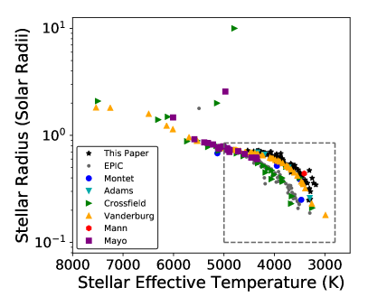
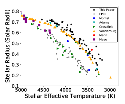
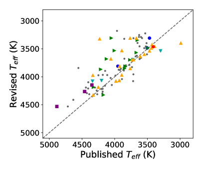
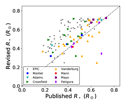
Figure 14: Comparison of our revised stellar parameters to earlier estimates from other studies. Top: Stellar radius versus effective temperature. Solid lines connect our revised estimates (black stars) to the the earlier estimates (colors) for each star. The right panel shows a zoomed-in view of the boxed region shown in the left panel. The errorbars are omitted from this figure for clarity; consult Figure 15 to see the errorbars. Bottom Left: Revised stellar effective temperatures versus previously published values. Bottom Right: Revised stellar radii versus previously published values.

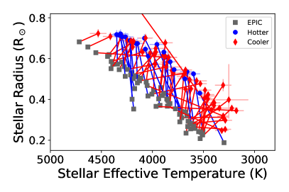
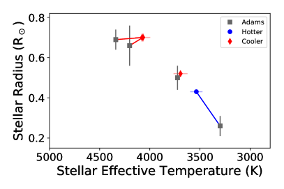
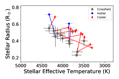
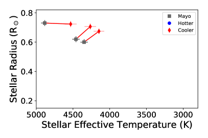
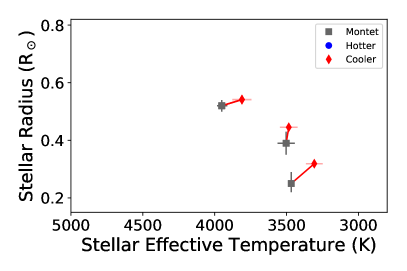
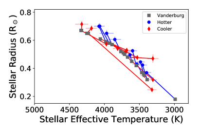
Figure 15: Comparison of our revised stellar parameters to earlier estimates from other studies. Solid lines connect our revised estimates (black stars) to the the earlier estimates (colors) for each star. The revised values are blue if the temperature estimate has increased and red if the temperature estimate has decreased. Top Left: Comparison to values published in the Ecliptic Plane Input Catalog (EPIC Huber et al., 2016). Top Right: Comparison to Adams et al. (2016). Middle Left: Comparison to Crossfield et al. (2016). Middle Right: Comparison to Mayo et al. (2018). Bottom Left: Comparison to Montet et al. (2015). Bottom Right: Comparison to Vanderburg et al. (2016).

For their K2 catalog, Montet et al. (2015) estimated stellar properties by using the isochrones Python module (Morton, 2015) to identify the stellar models in the Dartmouth Stellar Evolution Database (Dotter et al., 2008) that were most consistent with the archival photometry for each star. Dressing et al. (2017a) contained five stars from Montet et al. (2015); this cool dwarf sample includes three stars from Montet et al. (2015). Compared to the values published by Montet et al. (2015), we find that our revised radii are fairly consistent but that our temperature estimates differ by 18–160K. Our estimated $T_{\rm eff}$ are 140 K cooler for EPIC 201367065, 160 K cooler for EPIC 201465501, and 18 K cooler for EPIC 201912552.

Adams et al. (2016) adopted stellar effective temperatures from the K2-TESS Stellar Properties Catalog for most candidates. For candidates identified in Campaign 4, Adams et al. (2016) estimated temperatures from spectra they acquired using the Tull Coudé spectrograph (Tull et al., 1995) at the Harlan J. Smith 2.7-m telescope at McDonald Observatory. They estimated the radii of their targets using the radius-$T_{\rm eff}$ relations established by Boyajian et al. (2012). Four of the stars in our cool dwarf sample were previously published by Adams et al. (2016). Compared to the estimates published by Adams et al. (2016), our estimated stellar effective temperatures are between 240K hotter and 260K cooler with a median temperature difference of 82 K cooler. Our estimated radii are $0.02{\rm\,R_{\odot}}-0.17{\rm\,R_{\odot}}$ larger with a median difference of $0.03{\rm\,R_{\odot}}$ (5%).

For most targets, Crossfield et al. (2016) determined $T_{\rm eff}$, log $g$, and [Fe/H] by using SpecMatch to analyze spectra they obtained using the HIRES echelle spectrometer (Vogt et al., 1994) on the 10-m Keck I telescope, the Levy spectrograph (Vogt et al., 2014) at the Automated Planet Finder, and the FEROS echelle spectrograph (Kaufer & Pasquini, 1998) at the 2.2-m MPG telescope. They then determined masses and radii using by the isochrones Python package (Morton, 2015). A subset of the stars in the Crossfield et al. (2016) catalog did not have SpecMatch parameters. Those stars were assigned the stellar parameters from Huber et al. (2016) if they were included in the EPIC or from isochrones fits to broadband photometry from APASS, 2MASS, and WISE for stars not in the EPIC.

Like Montet et al. (2015), Crossfield et al. (2016) used Dartmouth stellar models (Dotter et al., 2008) for the isochrones analysis and therefore also underestimated the radii of cool dwarfs. In Dressing et al. (2017a), we found that our revised radius estimates were typically 28% ($0.10{\rm\,R_{\odot}}$) larger than the radii reported by Crossfield et al. (2016). The cool dwarf sample in this paper includes 12 stars from Crossfield et al. (2016). As in our 2017 paper, our radius estimates are typically $0.11{\rm\,R_{\odot}}$ (28%) larger. In addition, our temperature estimates are roughly 87K cooler than the Crossfield et al. (2016) estimates. The radius and temperature changes across the sample are relatively uniform, with nearly all stars moving upward and toward the right to larger radii and cooler temperatures.

Vanderburg et al. (2016) report a mix of spectroscopic and photometric parameters for their targets. For stars with spectroscopic estimates, Vanderburg et al. (2016) obtained optical spectra with the Tillinghast Reflector Echelle Spectrograph (TRES) on the 1.5-m telescope at Fred L. Whipple Observatory and analyzed the spectra using the Stellar Parameter Classification (SPC Buchhave et al., 2012, 2014) method. For stars without TRES spectra, Vanderburg et al. (2016) estimated stellar effective temperatures using a variety of color-temperature relations. Their preferred relation was the $V-K$ relation from Boyajian et al. (2013) but they defaulted to the $B-V$ or $g-r$ relations from Boyajian et al. (2013) or the $J-K$ relation from González Hernández & Bonifacio (2009) when necessary. For stars with colors beyond the validity range of those relations, Vanderburg et al. (2016) instead estimated temperatures by consulting the spectral type tables published by Pecaut & Mamajek (2013) or by applying the $V-K$ color-temperature relation from Casagrande et al. (2008) for the reddest stars. For stars cooler than 5778K, Vanderburg et al. (2016) then estimated stellar radii by applying the temperature-radius relationships from Boyajian et al. (2012). Dressing et al. (2017a) contained 9 stars from Vanderburg et al. (2016); we found that our revised radius estimates were 8% ($0.05{\rm\,R_{\odot}}$) larger than the radii reported by Vanderburg et al. (2016).

The cool dwarf sample in this paper contains 22 stars from Vanderburg et al. (2016). The median changes between our revised parameters and those published by Vanderburg et al. (2016) are that our radius estimates are $0.03{\rm\,R_{\odot}}$ (5%) larger and our stellar effective temperatures are 92 K hotter. Although most stars slightly upward to larger radii and moderately different temperatures, three stars (EPIC 201465501 (K2-9), EPIC 206032309, and EPIC 206215704) have extremely different parameter estimates in this paper than in Vanderburg et al. (2016).

The M3 dwarf EPIC 201465501 (K2-9) was previously estimated by Vanderburg et al. (2016) to have $R_{\star,pub}=0.52{\rm\,R_{\odot}}$ and $T_{{\rm eff},pub}=3765$K, but the revised radius is 40% smaller ($R_{\star}=0.32\pm 0.01{\rm\,R_{\odot}}$) and the revised temperature $T_{\rm eff}=3308\pm 58$K is 457K cooler. These revised estimates are consistent with the earlier classification by Schlieder et al. (2016) of K2-9 as an M2.5V$\pm 0.5$ star with $T_{\rm eff}=3390\pm 150$K and $R_{\star}=0.31\pm 0.11{\rm\,R_{\odot}}$ and close to the values of $T_{\rm eff}=3468^{+20}_{-19}$K and $R_{\star}=0.25^{+0.04}_{-0.03}{\rm\,R_{\odot}}$ reported by Montet et al. (2015) in the discovery paper. Our revised estimates are also consistent with the constraints of $T_{\rm eff}=3460\pm 164$K and $R_{\star}=0.366\pm 0.053{\rm\,R_{\odot}}$ published by Martinez et al. (2017).

EPIC 206032309, an M2 dwarf at a distance of $161\pm 1.8$ pc, was initially estimated to have $R_{\star,pub}=0.18{\rm\,R_{\odot}}$ and $T_{{\rm eff},pub}=2989$K, but our analysis suggests that the star is much hotter and larger ($R_{\star}=0.37\pm 0.01{\rm\,R_{\odot}}$, $T_{\rm eff}=3398\pm 66$K). Finally, we found that both the temperature and the radius were significantly overestimated for the M4 dwarf EPIC 206215704: the published values were $R_{\star,pub}=0.65{\rm\,R_{\odot}}$ and $T_{{\rm eff},pub}=4231$K while we find $R_{\star}=0.25\pm 0.01{\rm\,R_{\odot}}$ and $T_{\rm eff}=3321\pm 65$K.

Mann et al. (2017a) classified their target stars by acquiring optical spectra with the SuperNova Integral Field Spectrograph (SNIFS Aldering et al., 2002; Lantz et al., 2004) on the University of Hawai’i 2.2-m telescope on Mauna Kea and near-infrared spectra with SpeX on the IRTF and the Immersion Grating Infrared Spectrometer (IGRINS Park et al., 2014; Mace et al., 2016). They then confirmed that the stars were members of Praesepe and determined stellar effective temperatures by comparing their dereddened spectra to a grid of BT-SETTL CIFIST stellar models (Allard et al., 2012). Next, they estimated bolometric fluxes of by comparing their spectra to archival photometry and determined stellar radii using the Stefan-Boltzmann relation. Finally, Mann et al. (2017a) used the mass-$M_{K}$ relation they established in Mann et al. (2015) to determine stellar masses. EPIC 211916756 (K2-95) is the only star from Mann et al. (2017a) included in this paper. Our estimates of $R_{\star}=0.42\pm 0.01{\rm\,R_{\odot}}$, $T_{\rm eff}=3463\pm 76$K agree well with the previously published estimates of $R_{\star}=0.44\pm 0.02{\rm\,R_{\odot}}$ and $T_{\rm eff}=3410\pm 65$K from Mann et al. (2017a); $R_{\star}=0.402\pm 0.050{\rm\,R_{\odot}}$ and $T_{\rm eff}=3471\pm 124$K from Obermeier et al. (2016); $R_{\star}=0.44\pm 0.03{\rm\,R_{\odot}}$ and $T_{\rm eff}=3325\pm 100$K from Pepper et al. (2017); and $R_{\star}=0.42\pm 0.09{\rm\,R_{\odot}}$ and $T_{\rm eff}=3704\pm 214$K from Martinez et al. (2017).

Like Vanderburg et al. (2016), Mayo et al. (2018) estimated spectroscopic stellar parameters by obtaining TRES spectra and running SPC. Three stars from Mayo et al. (2018) are in our cool dwarf sample. As shown in Figure 15, our radius estimates are significantly larger for two stars (EPIC 201110617 = K2-156 and EPIC 220321605 = K2-212), but our radius estimate for EPIC 201390048 (K2-162) is consistent with that from Mayo et al. (2018). Our temperature estimates for K2-156 and K2-212 are nearly 200K cooler than those estimated by Mayo et al. (2018) and our estimate for K2-162 is roughly 350K cooler.

6 Conclusions

This paper is the fourth in a series of papers about cool dwarfs observed by the K2 mission. We presented NIR spectroscopy and revised classifications for 172 candidate cool dwarfs observed by K2 during campaigns 1 – 17. While 86 (50%) of our target stars were indeed cool dwarfs, our sample also included 74 hotter stars and 12 giant stars.

For the cool dwarfs, we estimated stellar properties from our NIR spectra using empirical relations developed by Newton et al. (2014, 2015) and Mann et al. (2013a, b). We also determine photometric properties by combining parallaxes and inferred distances from Gaia DR2 with archival photometry. We found that the radius and effective temperature estimates from both methods agreed well. However, the stellar effective temperatures reported by the Gaia team were approximately 200K hotter than our photometric or spectroscopics estimates.

The spectroscopic and photometric mass estimates are correlated, but the slope of the relation is shallower than a 1:1 line, which causes the photometric mass estimates to be larger than the spectroscopic mass estimates for the least massive stars and smaller than the spectroscopic mass estimates for the most massive stars. For the eleven stars with photometric mass estimates below $0.4{\rm\,M_{\odot}}$, the photometric estimates were systematically $0.11{\rm\,M_{\odot}}$ (34%) higher than the spectroscopic mass estimates. For stars with photometric masses $0.4{\rm\,M_{\odot}}<M_{\rm phot}<0.6{\rm\,M_{\odot}}$, the offset persists, but the difference is smaller: the photometric masses are roughly $0.03{\rm\,M_{\odot}}$ (6%) higher than the spectroscopic masses. Finally, for the most massive cool dwarfs ($M_{\rm phot}>0.6{\rm\,M_{\odot}}$), we found that the photometric mass estimates were $0.02{\rm\,M_{\odot}}$ (3%) lower than the spectroscopic mass estimates. The offset between the spectroscopic and photometric mass estimates could be partially explained by unresolved binaries.

Our cool dwarf sample extended from K5 to M4. Eleven of the 86 cool dwarfs have candidate stellar companions within $1"$ revealed by AO or speckle imaging (3 stars) or were identified as possible eclipsing binaries (8 stars). For the remaining 75 stars that are presumed to be single or in wide binaries, we found that the distribution of stellar radii extends from $0.24{\rm\,R_{\odot}}-0.74{\rm\,R_{\odot}}$ with a median value of $0.58{\rm\,R_{\odot}}$, the stellar masses range from $0.22{\rm\,M_{\odot}}$ to $0.75{\rm\,M_{\odot}}$ with a median value of $0.58{\rm\,M_{\odot}}$, and the stellar effective temperatures span 3077 – 4730K with a median value of 3693K. The typical star in the sample is slightly metal-poor (median [Fe/H]$=-0.06$), but the sample extends from [Fe/H]$=-0.42$ to [Fe/H]$=0.50$.

Compared to the original stellar radii published in the EPIC, our revised radii tend to be larger. The median increase in the estimated stellar radius is $0.15{\rm\,R_{\odot}}$ (40%). This increase is nearly identical to the difference of $0.13{\rm\,R_{\odot}}$ (39%) we found in Dressing et al. (2017a) between our revised stellar radii and the original EPIC estimates for the first set of stars considered as part of this project. In addition to the change in the radius estimates, we find that the stellar effective temperatures in the EPIC are overestimated by roughly 65K relative to our revised values.

Extending the comparison to previously published K2 planet candidate catalogs (Adams et al., 2016; Crossfield et al., 2016; Mayo et al., 2018; Montet et al., 2015; Vanderburg et al., 2016), we find that other previous studies have also tended to underestimate stellar radii and overestimate stellar effective temperatures. The radii and equilibrium temperatures of transiting planets are derived from their transit depths and the properties of their host stars, so systematic errors in stellar properties will lead to corresponding errors in planetary properties. Ignoring any possible systematic over- or under-estimates of the planet/star radius ratios, we anticipate the radii of any associated planets are also 5–40% larger than previously calculated using catalogs that relied on theoretical models to estimate stellar properties.

Table 1: Spectral Indices and Gaia Crossmatches for Targets Classified as Evolved Stars

EPIC			Gaia DR2					This Work
EPIC	$Kp$	$Ks$	Designation	PM RA	PM Dec	Parallax	Distance	Instrument	EW K I	EW Na I	EW Ca II
201231064	12.358	10.261	3598019894861833856	-0.384758	-16.393264	1.062600	916.318517	TSPEC	$\cdots$	$\cdots$	$\cdots$
201516974	11.238	9.270	3798898062211776256	-5.199212	-37.565546	1.233189	792.410202	TSPEC	$\cdots$	$\cdots$	$\cdots$
203776696	15.037	11.853	6049057713786919936	7.634639	0.802432	0.939381	1038.411156	TSPEC	$\cdots$	$\cdots$	$\cdots$
205084841	15.605	12.612	4131264587452082944	-3.982365	-2.197555	1.159403	843.771463	TSPEC	$\cdots$	$\cdots$	$\cdots$
206311743	12.922	10.701	2616298436668399616	7.075691	-36.846634	1.494429	656.665138	TSPEC	$\cdots$	$\cdots$	$\cdots$
211333233	9.653	5.883	600784874384342400	-1.802325	3.770199	0.774226	1239.495584	SpeX	2.295561	-0.755824	13.595743
214741009	14.012	11.788	4073371142719483264	-3.310084	-0.777168	0.138980	4885.770766	SpeX	-0.434720	-0.465135	5.117540
214741009	14.012	11.788	4073371142719483136	$\cdots$	$\cdots$	$\cdots$	$\cdots$	SpeX	-0.434720	-0.465135	5.117540
214741009	14.012	11.788	4073371142719466624	$\cdots$	$\cdots$	$\cdots$	$\cdots$	SpeX	-0.434720	-0.465135	5.117540
214741009	14.012	11.788	4073371142759019264	2.958019	-12.659866	0.311834	2948.777338	SpeX	-0.434720	-0.465135	5.117540
224588736	9.178	6.405	4110568686336849152	6.335847	-1.498865	2.928539	338.334113	SpeX	0.042580	0.470931	8.354823
224685166	13.504	9.620	4116398537524530816	$\cdots$	$\cdots$	$\cdots$	$\cdots$	SpeX	$\cdots$	$\cdots$	$\cdots$
224685166	13.504	9.620	4116398537524581888	$\cdots$	$\cdots$	$\cdots$	$\cdots$	SpeX	$\cdots$	$\cdots$	$\cdots$
224685166	13.504	9.620	4116398537496365824	2.706530	-6.092524	-0.114821	7127.918387	SpeX	$\cdots$	$\cdots$	$\cdots$
224685166	13.504	9.620	4116398537496365184	-0.112218	-8.934496	0.632351	$\cdots$	SpeX	$\cdots$	$\cdots$	$\cdots$
230731829	12.252	9.567	4128103074906953728	-3.668148	-0.442521	0.853148	1138.334242	SpeX	0.408937	0.304515	5.893129
233511840	12.355	9.899	4134987121538080512	-0.326771	-4.912940	-0.161470	4422.269051	SpeX	0.324789	-0.102504	7.453629
233511840	12.355	9.899	4134987121548634496	-14.137402	-2.961014	0.878995	1105.389257	SpeX	0.324789	-0.102504	7.453629
234563958	13.615	10.578	4122446950889378176	-3.617409	-3.522856	-0.965834	5490.103811	SpeX	-0.140359	1.497482	7.110041
234563958	13.615	10.578	4122446950911274624	-2.114598	-3.068457	0.074967	$\cdots$	SpeX	-0.140359	1.497482	7.110041

Table 2: Candidate Stellar Companions Identified in Gaia DR2

Primary							Secondary						Analysis
		RA	Dec	$\mu_{\rm RA}$	$\mu_{\rm Dec}$	$\pi$		RA	Dec	$\mu_{\rm RA}$	$\mu_{\rm Dec}$	$\pi$	$\Delta\theta$	$\Delta\mu$	Cut	Bound
EPIC	Designation	(∘)	(∘)	mas/yr	mas/yr	mas	Designation	(∘)	(∘)	mas/yr	mas/yr	mas	($"$)	mas/yr	mas/yr	Pair?
201119435	3595791498326534144	180.104930	-6.052428	-28.7	-8.19	1.79	3595791498324496384	180.105224	-6.052890	-27.6	-7.31	-0.08	1.97	1.42	1.0	no
201650711	3812335125095532672	172.044400	2.826726	80.2	-28.8	10.91	3812335125094701056	172.044175	2.827166	80.1	-29.1	10.84	1.78	0.38	65.2	yes
202071401	3378104379464943616	100.378771	20.921884	178.3	-208.6	7.83	3378104379464943104	100.379545	20.922202	177.8	-208.9	7.82	2.93	0.58	3051	yes
202071401	3378104379464943616	100.378771	20.921884	178.3	-208.6	7.83	3378104379464943232	100.378110	20.923489	-0.95	-2.709	0.72	6.22	272.96	107	no
202071635	3373469800514670976	93.571792	18.627016	-0.19	-1.49	0.34	3373469800511625856	93.571783	18.625649	-0.29	-2.036	0.87	4.92	0.55	0.00001	no
202086968	3369361402301215616	97.005609	16.388881	-3.87	-4.41	1.96	3369361406595494016	97.005521	16.388346	-4.20	-4.15	1.94	1.95	0.42	0.002	no
205040048	6245720108744660480	242.168354	-19.696900	-33.3	-237.8	10.96	6245720104449034880	242.167800	-19.695982	3.57	-6.05	0.29	3.83	234.70	124	no
205111664	6245607576304205952	243.680091	-19.346884	-3.95	-67.2	5.36	6245607580597734912	243.679158	-19.346593	$\cdots$	$\cdots$	$\cdots$	3.43	$\cdots$	$\cdots$	unknown
210693462	44838019758175488	55.444208	18.268697	187.1	-69.6	14.28	44838019756570112	55.444286	18.268491	185.5	-74.1	15.22	0.79	4.75	3169	yes
211089792	150054788545735424	62.670422	24.401656	16.5	-22.0	5.57	150054788545735296	62.671157	24.402648	14.9	-22.6	14.01	5.48	1.63	0.3	no
211783206	658478104919190400	130.145810	17.077987	$\cdots$	$\cdots$	$\cdots$	658478036198719360	130.146335	17.076670	4.77	-8.33	19.98	0.46	$\cdots$	0.005	unknown
214741009	4073371142759019264	281.115761	-25.753800	2.96	-12.7	0.31	4073371142719483264	281.115606	-25.752627	-3.31	-0.78	0.14	4.26	13.44	0.003	no
214741009	4073371142759019264	281.115761	-25.753800	2.96	-12.7	0.31	4073371142719483136	281.115795	-25.752758	$\cdots$	$\cdots$	$\cdots$	3.75	$\cdots$	$\cdots$	unknown
214741009	4073371142759019264	281.115761	-25.753800	2.96	-12.7	0.31	4073371142719466624	281.116989	-25.754003	$\cdots$	$\cdots$	$\cdots$	4.26	$\cdots$	$\cdots$	unknown
224685166	4116398537496365184	264.542000	-23.812946	-0.11	-8.93	0.63	4116398537496365824	264.542637	-23.813633	2.71	-6.09	-0.11	3.30	4.00	0.004	no
224685166	4116398537496365184	264.542000	-23.812946	-0.11	-8.93	0.63	4116398537524581888	264.542474	-23.812090	$\cdots$	$\cdots$	$\cdots$	3.49	$\cdots$	$\cdots$	unknown
224685166	4116398537496365184	264.542000	-23.812946	-0.11	-8.93	0.63	4116398537524530816	264.541299	-23.812611	$\cdots$	$\cdots$	$\cdots$	2.70	$\cdots$	$\cdots$	unknown
227560005	4124196681900615040	262.758677	-17.843539	10.9	-85.8	15.45	4124196686196694656	262.759848	-17.843199	-0.74	-4.68	-1.15	4.29	81.95	2.5	no
227560005	4124196681900615040	262.758677	-17.843539	10.9	-85.8	15.45	4124196686190833536	262.757699	-17.842846	$\cdots$	$\cdots$	$\cdots$	4.25	$\cdots$	$\cdots$	unknown
227560005	4124196681900615040	262.758677	-17.843539	10.9	-85.8	15.45	4124196686190833408	262.758317	-17.842985	$\cdots$	$\cdots$	$\cdots$	2.36	$\cdots$	$\cdots$	unknown
230517842	4127572427427088000	255.599743	-21.714297	-106.0	-103.4	10.28	4127572427404873600	255.599677	-21.712924	-5.34	-1.00	0.34	4.95	143.58	13.7	no
233511840	4134987121548634496	260.278659	-17.259871	-14.1	-2.96	0.88	4134987121538080512	260.279300	-17.261058	-0.33	-4.91	-0.16	4.83	13.95	0.005	no
234563958	4122446950911274624	259.838536	-18.563837	-2.11	-3.07	0.07	4122446950889378176	259.839934	-18.563667	-3.62	-3.52	-0.97	4.94	1.57	0.0003	no
247363044	144383232692533248	68.104945	21.094725	-5.08	-17.0	2.38	144383232690201344	68.106230	21.094449	0.69	0.62	0.28	4.58	18.57	0.006	no

Table 3: Observing Conditions

			Date	Seeing
Semester	Instrument	Program	(UT)	(”)	Weather Conditions	K2OIs
2016A	TSPEC	P08	2016 Mar 27	$0\farcs 7-1\farcs 2$	clear	3
	TSPEC	P08	2016 Mar 28	$0\farcs 8-2\farcs 1$	mostly clear	25
2016B	SpeX	057	2016 Aug 7	$0\farcs 5-0\farcs 8$	closed part of night because of high humidity	6
	SpeX	057	2016 Aug 09	$0\farcs 7-1\farcs 3$	clear	9
	SpeX	057	2016 Aug 10	$0\farcs 4-1\farcs 2$	clear	3
	SpeX	057	2016 Sep 05	$0\farcs 3-0\farcs 5$	cirrus	4
	SpeX	057	2016 Sep 27	$0\farcs 3-0\farcs 6$	clear	1
	SpeX	057	2016 Sep 28	$0\farcs 5-0\farcs 7$	humid	3
	SpeX	057	2016 Oct 09	$0\farcs 4-0\farcs 8$	cirrus	3
	SpeX	057	2016 Oct 26	$0\farcs 5-0\farcs 7$	clear	4
	SpeX	057	2016 Oct 27	$0\farcs 4-1\farcs 1$	clear	3
	SpeX	057	2016 Nov 19	$0\farcs 6-0\farcs 9$	cirrus	2
2017A	SpeX	019	2017 Feb 11	$1\farcs 0-1\farcs 4$	cloudy	7
	TSPEC	P11	2017 May 12	$1\farcs 2$	clear	3
	TSPEC	P11	2017 May 13	$1\farcs 4$	clear	7
	TSPEC	P11	2017 May 14	$1\farcs 4$	clear then cloudy	27
	TSPEC	P11	2017 May 15	$1\farcs 3-1\farcs 5$	clear, then foggy; closed early because of high humidity	23
	TSPEC	P11	2017 Jul 06	$1\farcs 2$	mostly clear then partly cloudy	3
	TSPEC	P11	2017 Jul 07	$1\farcs 4$	clear, then mostly clear	4
	SpeX	019	2017 Jul 11	$0\farcs 4-0\farcs 7$	cirrus	4
	SpeX	019	2017 Jul 12	$0\farcs 5-0\farcs 9$	humid	2
	SpeX	019	2017 Jul 13	$0\farcs 5-1\farcs 5$	clear	1
	SpeX	019	2017 Jul 17	$0\farcs 4-0\farcs 7$	thin cirrus	1
	SpeX	019	2017 Jul 24	$0\farcs 4-0\farcs 7$	clear	1
	SpeX	019	2017 Jul 31	$0\farcs 7$ - 1$\farcs$0	clear	10
2017B	TSPEC	P08	2017 Aug 13	$1\farcs 0-1\farcs 2$	clear	10
	SpeX	064	2017 Sep 27	$0\farcs 5-0\farcs 9$	clear	4
	SpeX	064	2017 Sep 28	$0\farcs 9-1\farcs 4$	clear	2
	TSPEC	P08	2017 Oct 09	$1\farcs 0-3\farcs 0$	clear; closed early because of heavy particulates	11
	TSPEC	P08	2017 Dec 01	$1\farcs 6$	partly cloudy	8
	TSPEC	P08	2018 Jan 28	$2\farcs 8-4\farcs 5$	mostly clear	6
2018A	SpeX	073	2018 May 12	$0\farcs 5-0\farcs 6$	cirrus	4
	SpeX	073	2018 May 14	$0\farcs 6$ - 1$\farcs$0	cirrus	2
	SpeX	073	2018 June 3	$0\farcs 4-0\farcs 9$	clear at start then patchy clouds	9

Table 4: Stellar Classifications

				EPIC		Follow-Up Imaging				Gaia
	K2	Spectral						Eclipsing	Nearby			Parallax	Distance	Flags
EPIC	Name	Type	Campaign	$Kp$	$Ks$	Speckle	AO	Binary	Star	Match	Designation	(mas)	(pc)	AF	EF	VF	VP
201110617	K2-156	K5V	10	12.947	10.391	y	y	$\cdots$	$\cdots$	y	3596250888028092160	6.63	150	$\cdots$	$\cdots$	$\cdots$	10
201111557	$\cdots$	K4V	10	11.363	9.220	y	$\cdots$	$\cdots$	$\cdots$	y	3596276829630866432	10.26	97	$\cdots$	$\cdots$	$\cdots$	11
201119435	$\cdots$	K5V	10	15.082	12.714	$\cdots$	y	$\cdots$	y	y	3595791498326534144	1.79	551	$\cdots$	$\cdots$	$\cdots$	11
201119435	$\cdots$	K5V	10	15.082	12.714	$\cdots$	y	$\cdots$	y	close	3595791498324496384	-0.08	1473	$\cdots$	$\cdots$	$\cdots$	10
201127519	$\cdots$	K4V	10	11.558	9.430	y	y	y	y	y	3597255188821238016	8.47	118	$\cdots$	$\cdots$	$\cdots$	11
201155177	K2-42	K5V	1	14.632	12.284	$\cdots$	y	$\cdots$	$\cdots$	y	3599651986730350464	2.49	397	$\cdots$	$\cdots$	$\cdots$	10
201231064	K2-161	K1III	10	12.358	10.261	y	$\cdots$	$\cdots$	$\cdots$	y	3598019894861833856	1.06	916	$\cdots$	$\cdots$	$\cdots$	11
201264302	$\cdots$	M2V	1	13.879	10.357	$\cdots$	$\cdots$	$\cdots$	$\cdots$	y	3790435155572409856	13.88	72	$\cdots$	$\cdots$	$\cdots$	10
201352100	$\cdots$	K2V	10	12.798	10.708	y	y	$\cdots$	y	y	3694587531524362240	5.12	194	$\cdots$	$\cdots$	$\cdots$	12
201367065	K2-3	M1V	1	11.574	8.561	$\cdots$	y	$\cdots$	$\cdots$	y	3796690380302214272	22.66	44	$\cdots$	$\cdots$	y	9
201390048	K2-162	K5V	10	11.961	9.898	y	$\cdots$	$\cdots$	$\cdots$	y	3694878833385971840	8.01	124	$\cdots$	$\cdots$	$\cdots$	12
201427874	K2-163	K3V	10	12.819	10.627	y	y	$\cdots$	$\cdots$	y	3697972721667206144	4.77	209	$\cdots$	$\cdots$	y	7
201445392	K2-8	K3V	1	14.384	12.245	$\cdots$	y	$\cdots$	$\cdots$	y	3797977118144236288	2.45	404	$\cdots$	$\cdots$	y	8
201465501	K2-9	M3V	1	14.957	11.495	$\cdots$	y	$\cdots$	$\cdots$	y	3795633852707093120	12.02	83	$\cdots$	$\cdots$	$\cdots$	10
201516974	$\cdots$	G4III	1	11.238	9.270	$\cdots$	$\cdots$	$\cdots$	$\cdots$	y	3798898062211776256	1.23	792	$\cdots$	$\cdots$	y	9
201596733	$\cdots$	M1V	1	14.284	10.763	$\cdots$	$\cdots$	$\cdots$	$\cdots$	y	3810767049715469056	8.82	113	$\cdots$	$\cdots$	y	9
201650711	$\cdots$	K7V	1	12.254	9.309	$\cdots$	$\cdots$	$\cdots$	$\cdots$	y	3812335125095532672	10.91	91	$\cdots$	$\cdots$	y	9
201650711	$\cdots$	K7V	1	12.254	9.309	$\cdots$	$\cdots$	$\cdots$	$\cdots$	close	3812335125094701056	10.84	92	$\cdots$	$\cdots$	y	9
201663913	$\cdots$	M1V	14	14.451	11.333	$\cdots$	$\cdots$	$\cdots$	$\cdots$	y	3811688440459523456	4.63	215	$\cdots$	$\cdots$	$\cdots$	10
201677835	K2-48	K2V	1	14.019	11.838	y	y	$\cdots$	$\cdots$	y	3799841752426128896	3.16	314	$\cdots$	$\cdots$	$\cdots$	10
201690160	$\cdots$	K5V	14	12.755	10.253	$\cdots$	$\cdots$	$\cdots$	$\cdots$	y	3814764182504124416	7.03	142	$\cdots$	$\cdots$	y	9
201690311	K2-49	K7V	1	15.288	12.729	$\cdots$	$\cdots$	$\cdots$	$\cdots$	y	3895843479901597440	2.16	457	$\cdots$	$\cdots$	$\cdots$	10
201736247	K2-15	K3V	1	14.403	12.495	y	$\cdots$	$\cdots$	$\cdots$	y	3896271842760486272	2.00	494	$\cdots$	$\cdots$	$\cdots$	11
201785059	$\cdots$	M2V	1	14.595	10.854	$\cdots$	$\cdots$	$\cdots$	$\cdots$	y	3813693502991916416	11.34	88	$\cdots$	$\cdots$	$\cdots$	10
201831831	$\cdots$	K4V	14	12.862	10.633	$\cdots$	$\cdots$	$\cdots$	$\cdots$	y	3864275848232907776	5.26	189	$\cdots$	$\cdots$	$\cdots$	10
201833600	K2-50	K5V	1	14.252	11.664	$\cdots$	y	$\cdots$	$\cdots$	y	3817000078053804672	3.86	257	$\cdots$	$\cdots$	y	8
201912552	K2-18	M3V	1	12.473	8.899	$\cdots$	y	$\cdots$	$\cdots$	y	3910747531814692736	26.27	38	$\cdots$	$\cdots$	$\cdots$	10
201928106	$\cdots$	M3V	1	16.733	13.124	$\cdots$	y	$\cdots$	$\cdots$	y	3913913163229896064	3.27	303	$\cdots$	$\cdots$	$\cdots$	10
202071289	$\cdots$	G2V	0	11.000	$\cdots$	$\cdots$	y	$\cdots$	$\cdots$	y	3425807855371050624	3.76	265	$\cdots$	$\cdots$	$\cdots$	10
202071401	$\cdots$	K5V	0	12.900	10.107	y	y	$\cdots$	y	y	3378104379464943616	7.83	127	$\cdots$	$\cdots$	$\cdots$	10
202071401	$\cdots$	K5V	0	12.900	10.107	y	y	$\cdots$	y	close	3378104379464943232	0.72	1364	$\cdots$	$\cdots$	$\cdots$	10
202071401	$\cdots$	K5V	0	12.900	10.107	y	y	$\cdots$	y	close	3378104379464943104	7.82	128	$\cdots$	$\cdots$	$\cdots$	10
202071635	$\cdots$	F2V	0	10.200	$\cdots$	y	$\cdots$	y	$\cdots$	close	3373469800511625856	0.87	1241	$\cdots$	$\cdots$	y	8
202071635	$\cdots$	F2V	0	10.200	$\cdots$	y	$\cdots$	y	$\cdots$	y	3373469800514670976	0.34	2668	$\cdots$	$\cdots$	$\cdots$	11
202071645	$\cdots$	F2V	0	10.400	$\cdots$	$\cdots$	y	$\cdots$	$\cdots$	y	3371227617129676160	2.47	401	$\cdots$	$\cdots$	$\cdots$	10
202072965	$\cdots$	F2V	0	10.300	$\cdots$	y	$\cdots$	y	$\cdots$	y	3432818753826529792	2.09	471	$\cdots$	$\cdots$	$\cdots$	10
202083828	K2-26	M1V	0	14.000	10.530	y	y	$\cdots$	$\cdots$	y	3425691139632545152	10.07	99	$\cdots$	$\cdots$	y	9
202086968	$\cdots$	G2V	0	12.400	$\cdots$	y	$\cdots$	y	$\cdots$	close	3369361406595494016	1.94	509	$\cdots$	$\cdots$	$\cdots$	11
202086968	$\cdots$	G2V	0	12.400	$\cdots$	y	$\cdots$	y	$\cdots$	y	3369361402301215616	1.96	502	$\cdots$	$\cdots$	$\cdots$	11
202088212	$\cdots$	G5V	0	11.600	$\cdots$	y	y	$\cdots$	$\cdots$	y	3368700905049734784	2.36	419	$\cdots$	$\cdots$	$\cdots$	11
202089657	$\cdots$	G5V	10	11.600	$\cdots$	y	y	$\cdots$	$\cdots$	y	3426117131673547392	2.53	391	$\cdots$	$\cdots$	$\cdots$	11
202091388	$\cdots$	G8V	0	13.500	$\cdots$	y	$\cdots$	$\cdots$	$\cdots$	y	3423330522531466112	2.28	434	$\cdots$	$\cdots$	y	9
202093020	$\cdots$	G8V	0	14.800	$\cdots$	$\cdots$	$\cdots$	$\cdots$	$\cdots$	y	3369441018113246976	1.67	604	$\cdots$	$\cdots$	$\cdots$	10
202126888	$\cdots$	G5V	0	13.500	$\cdots$	y	y	$\cdots$	$\cdots$	y	3432489935426363520	0.86	1120	$\cdots$	$\cdots$	$\cdots$	11
203776696	K2-52	F2III	2	15.037	11.853	$\cdots$	y	$\cdots$	$\cdots$	y	6049057713786919936	0.94	1038	$\cdots$	$\cdots$	$\cdots$	10
204576757	$\cdots$	G4V	2	13.668	11.193	$\cdots$	$\cdots$	y	$\cdots$	y	6051922594416652416	2.33	423	$\cdots$	$\cdots$	$\cdots$	11
204658292	$\cdots$	K3V	2	14.421	12.073	$\cdots$	$\cdots$	$\cdots$	$\cdots$	y	6243022938002285568	2.70	367	$\cdots$	$\cdots$	$\cdots$	10
204884005	$\cdots$	K3V	2	11.514	9.417	$\cdots$	$\cdots$	$\cdots$	$\cdots$	y	4130211147935185024	8.58	116	$\cdots$	$\cdots$	$\cdots$	11
204888276	$\cdots$	M2V	2	12.542	9.251	$\cdots$	$\cdots$	$\cdots$	$\cdots$	$\cdots$	$\cdots$	$\cdots$	$\cdots$	$\cdots$	$\cdots$	$\cdots$	$\cdots$
204890128	K2-53	K2V	2	11.888	9.664	$\cdots$	y	$\cdots$	$\cdots$	y	6244643373326639360	7.22	138	$\cdots$	$\cdots$	$\cdots$	10
205040048	$\cdots$	M4V	2	14.989	11.453	$\cdots$	$\cdots$	$\cdots$	$\cdots$	close	6245720104449034880	0.29	3437	$\cdots$	$\cdots$	y	9
205040048	$\cdots$	M4V	2	14.989	11.453	$\cdots$	$\cdots$	$\cdots$	$\cdots$	y	6245720108744660480	10.96	91	$\cdots$	$\cdots$	$\cdots$	10
205084841	$\cdots$	G5III	2	15.605	12.612	$\cdots$	y	$\cdots$	$\cdots$	y	4131264587452082944	1.16	844	$\cdots$	$\cdots$	$\cdots$	13
205111664	$\cdots$	K1V	2	12.129	9.875	$\cdots$	$\cdots$	$\cdots$	$\cdots$	close	6245607580597734912	$\cdots$	$\cdots$	y	y	y	7
205111664	$\cdots$	K1V	2	12.129	9.875	$\cdots$	$\cdots$	$\cdots$	$\cdots$	y	6245607576304205952	5.36	186	$\cdots$	$\cdots$	y	8
205152172	$\cdots$	K5V	2	13.486	10.524	$\cdots$	$\cdots$	$\cdots$	$\cdots$	y	6245213817998911744	6.31	158	$\cdots$	$\cdots$	y	9
205489894	$\cdots$	M3V	2	12.337	8.965	$\cdots$	$\cdots$	$\cdots$	$\cdots$	y	4324010075312779520	21.82	46	$\cdots$	$\cdots$	$\cdots$	11
205947214	$\cdots$	K7V	3	16.121	12.777	$\cdots$	$\cdots$	y	$\cdots$	y	2598609558025174656	1.67	589	$\cdots$	$\cdots$	y	9
205996447	$\cdots$	M1V	3	15.262	12.312	$\cdots$	$\cdots$	y	$\cdots$	y	2597595056685061248	2.19	451	$\cdots$	$\cdots$	y	9
205999468	$\cdots$	K2V	3	12.932	11.011	$\cdots$	y	$\cdots$	$\cdots$	y	2599429694915622912	4.07	244	$\cdots$	$\cdots$	y	9
206026136	K2-57	K5V	3	14.101	11.645	$\cdots$	y	$\cdots$	$\cdots$	y	2603155390066307456	3.76	264	$\cdots$	$\cdots$	$\cdots$	10
206027655	K2-59	K2V	3	13.869	11.838	$\cdots$	y	$\cdots$	$\cdots$	y	2597903091739512320	3.18	311	$\cdots$	$\cdots$	y	6
206029450	$\cdots$	M0V	3	15.504	12.834	$\cdots$	$\cdots$	$\cdots$	$\cdots$	y	2599641660141170816	2.94	337	$\cdots$	$\cdots$	y	8
206032309	$\cdots$	M2V	3	15.782	12.538	$\cdots$	$\cdots$	$\cdots$	$\cdots$	y	2597400855444243840	6.17	161	$\cdots$	$\cdots$	y	8
206042996	$\cdots$	K5V	3	16.061	13.071	$\cdots$	$\cdots$	$\cdots$	$\cdots$	y	2600942622915012608	2.19	452	$\cdots$	$\cdots$	y	8
206055981	$\cdots$	K3V	3	13.418	10.957	y	$\cdots$	$\cdots$	$\cdots$	y	2601048588348190976	5.62	177	$\cdots$	$\cdots$	y	6
206061524	$\cdots$	K7V	3	14.443	11.579	$\cdots$	y	$\cdots$	y	y	2600505429604015872	3.51	283	$\cdots$	$\cdots$	y	8
206065006	$\cdots$	M1V	3	16.473	13.598	$\cdots$	y	$\cdots$	$\cdots$	y	2600521647400551552	2.12	467	$\cdots$	$\cdots$	y	7
206114294	$\cdots$	M1V	3	15.737	12.604	$\cdots$	y	$\cdots$	$\cdots$	y	2613060374924695552	3.07	323	$\cdots$	$\cdots$	y	6
206135682	$\cdots$	K3V	3	13.213	11.042	$\cdots$	$\cdots$	$\cdots$	$\cdots$	y	2613924969021549440	4.81	207	$\cdots$	$\cdots$	y	7
206159027	K2-68	K2V	3	12.597	10.530	$\cdots$	y	$\cdots$	$\cdots$	y	2614734243939231232	5.90	169	$\cdots$	$\cdots$	$\cdots$	10
206162305	K2-69	M1V	3	14.807	11.766	$\cdots$	y	$\cdots$	$\cdots$	y	2614926005638892032	5.51	181	$\cdots$	$\cdots$	y	9
206192813	K2-71	M3V	3	14.875	11.732	$\cdots$	y	$\cdots$	$\cdots$	y	2608279114251674624	6.50	153	$\cdots$	$\cdots$	$\cdots$	10
206215704	$\cdots$	M4V	3	15.598	12.767	$\cdots$	$\cdots$	$\cdots$	$\cdots$	y	2615281560211505408	9.07	110	$\cdots$	$\cdots$	y	9
206298289	$\cdots$	M1V	3	14.688	11.395	$\cdots$	$\cdots$	$\cdots$	$\cdots$	y	2621428856708032256	6.63	150	$\cdots$	$\cdots$	y	7
206311743	$\cdots$	G8III	3	12.922	10.701	$\cdots$	$\cdots$	$\cdots$	$\cdots$	y	2616298436668399616	1.49	657	$\cdots$	$\cdots$	$\cdots$	10
206317286	$\cdots$	K1V	3	13.806	11.635	$\cdots$	$\cdots$	$\cdots$	$\cdots$	y	2621545958991110144	3.15	314	$\cdots$	$\cdots$	y	9
206417197	$\cdots$	K1V	3	13.352	11.394	$\cdots$	$\cdots$	$\cdots$	$\cdots$	y	2622888531408156928	3.36	295	$\cdots$	$\cdots$	y	9
210363145	K2-77	K4V	4	11.896	9.799	y	y	$\cdots$	$\cdots$	y	37619725922094336	7.03	142	$\cdots$	$\cdots$	y	9
210400751	$\cdots$	K4V	4	11.892	9.890	y	y	$\cdots$	$\cdots$	y	37928001494790272	6.78	147	$\cdots$	$\cdots$	$\cdots$	11
210513446	$\cdots$	G4V	4	13.618	11.191	$\cdots$	y	$\cdots$	y	y	40328785134510080	3.12	318	$\cdots$	$\cdots$	$\cdots$	12
210559259	$\cdots$	K3V	4	13.699	11.323	$\cdots$	$\cdots$	$\cdots$	$\cdots$	y	40441583858056576	3.91	254	$\cdots$	$\cdots$	y	9
210659688	$\cdots$	M4V	4	16.499	12.694	$\cdots$	$\cdots$	$\cdots$	$\cdots$	y	44761741139048320	6.02	165	$\cdots$	$\cdots$	$\cdots$	10
210693462	K2-288	M2V	4	13.105	9.724	$\cdots$	y	$\cdots$	y	y	44838019758175488	14.29	70	$\cdots$	$\cdots$	$\cdots$	10
210693462	K2-288	M2V	4	13.105	9.724	$\cdots$	y	$\cdots$	y	close	44838019756570112	15.22	66	$\cdots$	$\cdots$	y	6
211089792	K2-29	K2V	4	12.914	$\cdots$	$\cdots$	y	$\cdots$	y	close	150054788545735296	5.48	182	$\cdots$	$\cdots$	$\cdots$	10
211089792	K2-29	K2V	4	12.914	$\cdots$	$\cdots$	y	$\cdots$	y	y	150054788545735424	5.57	178	$\cdots$	$\cdots$	$\cdots$	10
211333233	$\cdots$	M0III	5	9.653	5.883	$\cdots$	$\cdots$	$\cdots$	$\cdots$	y	600784874384342400	0.77	1239	$\cdots$	$\cdots$	$\cdots$	11
211383821	$\cdots$	K7V	5	14.044	11.506	$\cdots$	$\cdots$	$\cdots$	$\cdots$	y	601848888105730176	4.34	229	$\cdots$	$\cdots$	$\cdots$	12
211399359	$\cdots$	K3V	5	14.424	12.391	$\cdots$	y	y	$\cdots$	y	602466302541172736	2.23	443	$\cdots$	$\cdots$	$\cdots$	11
211529065	K2-270	K3V	5	13.431	11.368	$\cdots$	y	$\cdots$	$\cdots$	y	608395625151767680	3.54	281	$\cdots$	$\cdots$	$\cdots$	13
211541590	$\cdots$	M3V	5	14.336	10.648	$\cdots$	$\cdots$	$\cdots$	$\cdots$	y	606151109602008704	13.03	77	$\cdots$	$\cdots$	$\cdots$	11
211579683	$\cdots$	K3V	5	14.029	11.856	$\cdots$	$\cdots$	$\cdots$	$\cdots$	y	652028782028953856	2.73	363	$\cdots$	$\cdots$	$\cdots$	12
211631538	$\cdots$	K1V	16	14.221	12.173	$\cdots$	$\cdots$	$\cdots$	$\cdots$	y	609727889647633664	2.40	411	$\cdots$	$\cdots$	$\cdots$	13
211642882	$\cdots$	K4V	16	13.788	11.668	$\cdots$	$\cdots$	$\cdots$	$\cdots$	y	606804941063314816	3.20	310	$\cdots$	$\cdots$	$\cdots$	11
211741619	$\cdots$	K7V	16	13.564	10.489	$\cdots$	$\cdots$	$\cdots$	$\cdots$	y	610197278032980992	8.01	124	$\cdots$	$\cdots$	$\cdots$	14
211783206	$\cdots$	K5V	5	14.150	11.961	$\cdots$	$\cdots$	$\cdots$	$\cdots$	close	658478036198719360	0.46	1002	$\cdots$	$\cdots$	$\cdots$	12
211783206	$\cdots$	K5V	5	14.150	11.961	$\cdots$	$\cdots$	$\cdots$	$\cdots$	y	658478104919190400	$\cdots$	$\cdots$	y	y	$\cdots$	12
211797637	$\cdots$	K4V	5	13.713	11.261	$\cdots$	$\cdots$	$\cdots$	$\cdots$	y	658531465592884096	4.49	221	$\cdots$	$\cdots$	$\cdots$	13
211916756	K2-95	M3V	5	15.498	12.474	y	y	$\cdots$	$\cdots$	y	659744295638254336	5.54	180	$\cdots$	$\cdots$	$\cdots$	11
211925595	$\cdots$	K4V	5	14.466	12.427	$\cdots$	$\cdots$	$\cdots$	$\cdots$	y	660635243654126336	2.11	467	$\cdots$	$\cdots$	$\cdots$	14
212008766	K2-274	K1V	5	12.802	10.986	y	y	$\cdots$	$\cdots$	y	664406705976755712	4.35	228	$\cdots$	$\cdots$	$\cdots$	10
212009427	$\cdots$	M1V	5	14.072	10.767	$\cdots$	$\cdots$	y	$\cdots$	y	663140171661012480	5.43	183	$\cdots$	$\cdots$	$\cdots$	13
212048748	$\cdots$	M2V	16	12.771	9.190	$\cdots$	$\cdots$	$\cdots$	$\cdots$	y	684992690384102528	35.78	28	$\cdots$	$\cdots$	$\cdots$	11
212088059	$\cdots$	M1V	5	14.757	11.460	y	$\cdots$	$\cdots$	$\cdots$	y	685979983106267136	6.13	162	$\cdots$	$\cdots$	$\cdots$	14
212130773	K2-276	K3V	5	14.467	12.260	y	y	$\cdots$	$\cdots$	y	677884313351354880	2.02	488	$\cdots$	$\cdots$	$\cdots$	13
212204403	$\cdots$	K2V	16	12.482	10.381	$\cdots$	$\cdots$	$\cdots$	$\cdots$	y	690310993768911104	4.93	202	$\cdots$	$\cdots$	$\cdots$	13
212315941	$\cdots$	K5V	6	14.406	12.175	y	$\cdots$	y	y	y	3603756944672569856	1.15	852	$\cdots$	$\cdots$	$\cdots$	10
212330265	$\cdots$	M1V	6	14.949	11.655	$\cdots$	$\cdots$	$\cdots$	$\cdots$	y	6295480809559200512	5.61	178	$\cdots$	$\cdots$	$\cdots$	10
212354731	$\cdots$	M3V	6	15.805	12.507	y	$\cdots$	y	$\cdots$	y	3604723479817463424	6.19	161	$\cdots$	$\cdots$	y	8
212575828	$\cdots$	K3V	6	15.508	13.392	y	$\cdots$	$\cdots$	$\cdots$	y	3616517223789495424	1.43	688	$\cdots$	$\cdots$	$\cdots$	10
212737443	$\cdots$	K5V	6	14.461	12.160	y	$\cdots$	$\cdots$	$\cdots$	y	3630680754621236096	2.95	336	$\cdots$	$\cdots$	y	8
212748535	$\cdots$	M1V	$\cdots$	13.582	10.530	$\cdots$	$\cdots$	$\cdots$	$\cdots$	y	3632158841846331392	8.02	124	$\cdots$	$\cdots$	$\cdots$	10
212796016	$\cdots$	K7V	6	14.209	11.308	$\cdots$	$\cdots$	$\cdots$	$\cdots$	y	3632595897718444800	5.30	188	$\cdots$	$\cdots$	y	9
214741009	$\cdots$	G5III	7	14.012	11.788	$\cdots$	y	y	$\cdots$	y	4073371142759019264	0.31	2949	$\cdots$	$\cdots$	$\cdots$	11
214741009	$\cdots$	G5III	7	14.012	11.788	$\cdots$	y	y	$\cdots$	close	4073371142719483264	0.14	4886	$\cdots$	$\cdots$	$\cdots$	11
214741009	$\cdots$	G5III	7	14.012	11.788	$\cdots$	y	y	$\cdots$	close	4073371142719483136	$\cdots$	$\cdots$	y	y	y	4
214741009	$\cdots$	G5III	7	14.012	11.788	$\cdots$	y	y	$\cdots$	close	4073371142719466624	$\cdots$	$\cdots$	y	y	y	7
220187552	$\cdots$	M1V	8	12.836	9.886	y	y	y	y	y	2533763149653076352	$\cdots$	$\cdots$	y	y	y	9
220194953	$\cdots$	M1V	8	12.856	10.612	y	$\cdots$	$\cdots$	$\cdots$	y	2536443724641751680	8.03	124	$\cdots$	$\cdots$	y	9
220194974	K2-148	K7V	8	12.975	10.292	y	$\cdots$	$\cdots$	$\cdots$	y	2536443724641751808	8.01	124	$\cdots$	$\cdots$	y	9
220207765	$\cdots$	K2V	8	12.170	10.388	$\cdots$	$\cdots$	$\cdots$	$\cdots$	y	2534280156340927744	5.08	196	$\cdots$	$\cdots$	y	9
220241529	K2-209	K2V	8	10.717	8.613	y	$\cdots$	$\cdots$	$\cdots$	y	2537467988442521600	13.04	76	$\cdots$	$\cdots$	$\cdots$	10
220245303	$\cdots$	K2V	8	11.821	9.962	y	$\cdots$	$\cdots$	$\cdots$	y	2549435893337972352	6.63	150	$\cdots$	$\cdots$	$\cdots$	12
220256496	K2-211	K0V	8	12.872	11.104	y	$\cdots$	$\cdots$	$\cdots$	y	2559203924574351616	3.64	272	$\cdots$	$\cdots$	y	9
220292715	$\cdots$	K1V	8	12.213	10.205	y	$\cdots$	$\cdots$	$\cdots$	y	2538765201709897984	6.31	158	$\cdots$	$\cdots$	y	9
220321605	K2-212	K7V	8	12.588	9.856	y	y	$\cdots$	$\cdots$	y	2538824923230146560	9.13	109	$\cdots$	$\cdots$	y	9
220336320	$\cdots$	M2V	8	15.929	12.824	$\cdots$	y	y	$\cdots$	y	2539599116855026048	3.34	298	$\cdots$	$\cdots$	$\cdots$	11
220448185	$\cdots$	M4V	8	15.976	13.543	$\cdots$	$\cdots$	$\cdots$	$\cdots$	y	2564954125574046336	4.25	234	$\cdots$	$\cdots$	y	9
220481411	K2-216	K3V	8	12.100	9.721	y	y	$\cdots$	$\cdots$	y	2556231154370582400	8.63	115	$\cdots$	$\cdots$	$\cdots$	11
220501947	$\cdots$	K4V	8	13.539	11.135	y	y	y	$\cdots$	y	2564784633279953536	4.27	233	$\cdots$	$\cdots$	$\cdots$	10
220522262	K2-281	K2V	8	14.763	12.523	y	y	$\cdots$	$\cdots$	y	2577432178095422976	2.15	458	$\cdots$	$\cdots$	$\cdots$	11
220555384	$\cdots$	K7V	8	12.395	9.700	y	y	$\cdots$	y	y	2580690168487411840	6.85	147	$\cdots$	y	y	9
220565349	$\cdots$	G4V	8	14.122	12.204	y	y	y	$\cdots$	y	2578666551696182528	1.63	604	$\cdots$	$\cdots$	$\cdots$	10
220621087	K2-151	M2V	8	13.384	10.117	y	y	$\cdots$	$\cdots$	y	2579620343673729408	14.36	69	$\cdots$	$\cdots$	$\cdots$	10
220629489	K2-283	K2V	8	14.119	11.983	y	y	$\cdots$	$\cdots$	y	2581916673708201216	2.45	403	$\cdots$	$\cdots$	$\cdots$	11
220696233	$\cdots$	M0V	8	15.540	12.286	y	y	y	$\cdots$	y	2580505553613124992	3.73	266	$\cdots$	$\cdots$	$\cdots$	10
224588736	$\cdots$	K1III	11	9.178	6.405	$\cdots$	$\cdots$	$\cdots$	$\cdots$	y	4110568686336849152	2.93	338	$\cdots$	$\cdots$	$\cdots$	10
224685166	$\cdots$	M1III	11	13.504	9.620	$\cdots$	$\cdots$	$\cdots$	$\cdots$	close	4116398537524530816	$\cdots$	$\cdots$	y	$\cdots$	y	4
224685166	$\cdots$	M1III	11	13.504	9.620	$\cdots$	$\cdots$	$\cdots$	$\cdots$	close	4116398537524581888	$\cdots$	$\cdots$	y	y	y	4
224685166	$\cdots$	M1III	11	13.504	9.620	$\cdots$	$\cdots$	$\cdots$	$\cdots$	close	4116398537496365824	-0.11	7128	$\cdots$	$\cdots$	y	9
224685166	$\cdots$	M1III	11	13.504	9.620	$\cdots$	$\cdots$	$\cdots$	$\cdots$	y	4116398537496365184	0.63	1516	$\cdots$	$\cdots$	y	8
227560005	$\cdots$	M0V	11	12.039	9.029	y	$\cdots$	$\cdots$	$\cdots$	close	4124196686190833408	$\cdots$	$\cdots$	y	$\cdots$	y	4
227560005	$\cdots$	M0V	11	12.039	9.029	y	$\cdots$	$\cdots$	$\cdots$	y	4124196681900615040	15.45	65	$\cdots$	$\cdots$	$\cdots$	11
227560005	$\cdots$	M0V	11	12.039	9.029	y	$\cdots$	$\cdots$	$\cdots$	close	4124196686196694656	-1.15	5718	$\cdots$	$\cdots$	y	8
227560005	$\cdots$	M0V	11	12.039	9.029	y	$\cdots$	$\cdots$	$\cdots$	close	4124196686190833536	$\cdots$	$\cdots$	y	$\cdots$	y	5
228724232	K2-235	K7V	10	11.243	8.637	y	y	$\cdots$	$\cdots$	y	3578638842054261248	15.42	65	$\cdots$	$\cdots$	$\cdots$	12
228748826	K2-250	K3V	10	13.948	12.016	y	y	y	y	y	3582706794559052160	2.38	415	$\cdots$	$\cdots$	y	9
228845657	$\cdots$	K3V	10	14.040	11.878	y	y	y	y	y	3680925481073923840	3.00	331	$\cdots$	$\cdots$	$\cdots$	10
228974324	K2-257	M1V	10	12.873	9.661	y	$\cdots$	$\cdots$	$\cdots$	y	3695235654973028736	15.59	64	$\cdots$	$\cdots$	y	9
229133720	$\cdots$	K3V	10	11.477	9.362	y	y	$\cdots$	$\cdots$	y	3700298875955340672	9.51	105	$\cdots$	$\cdots$	$\cdots$	12
230517842	$\cdots$	K5V	11	12.261	9.604	$\cdots$	$\cdots$	$\cdots$	$\cdots$	close	4127572427404873600	0.34	3654	$\cdots$	$\cdots$	$\cdots$	10
230517842	$\cdots$	K5V	11	12.261	9.604	$\cdots$	$\cdots$	$\cdots$	$\cdots$	y	4127572427427088000	10.28	97	$\cdots$	$\cdots$	$\cdots$	11
230731829	$\cdots$	K0III	11	12.252	9.567	$\cdots$	$\cdots$	$\cdots$	$\cdots$	y	4128103074906953728	0.85	1138	$\cdots$	$\cdots$	$\cdots$	11
230778501	$\cdots$	K3V	11	12.388	9.874	y	$\cdots$	$\cdots$	$\cdots$	y	4128547488084332160	6.98	143	$\cdots$	$\cdots$	$\cdots$	10
233511840	$\cdots$	K0III	11	12.355	9.899	y	$\cdots$	$\cdots$	$\cdots$	close	4134987121538080512	-0.16	4422	y	y	y	7
233511840	$\cdots$	K0III	11	12.355	9.899	y	$\cdots$	$\cdots$	$\cdots$	y	4134987121548634496	0.88	1105	$\cdots$	$\cdots$	$\cdots$	11
234563958	$\cdots$	K4III	11	13.615	10.578	$\cdots$	$\cdots$	$\cdots$	$\cdots$	close	4122446950889378176	-0.97	5490	$\cdots$	$\cdots$	y	9
234563958	$\cdots$	K4III	11	13.615	10.578	$\cdots$	$\cdots$	$\cdots$	$\cdots$	y	4122446950911274624	0.07	8546	$\cdots$	$\cdots$	$\cdots$	11
245941309	$\cdots$	K3V	12	14.478	12.451	$\cdots$	y	y	$\cdots$	y	2436561167796845184	1.46	673	$\cdots$	$\cdots$	$\cdots$	10
245953291	$\cdots$	M0V	12	14.610	11.403	$\cdots$	y	$\cdots$	$\cdots$	y	2434055415156672384	5.09	195	$\cdots$	$\cdots$	$\cdots$	10
246004726	$\cdots$	K5V	12	12.872	10.253	y	y	$\cdots$	$\cdots$	y	2437219981420474752	7.56	132	$\cdots$	$\cdots$	y	8
246014919	$\cdots$	K7V	12	12.176	9.565	y	$\cdots$	$\cdots$	$\cdots$	y	2435914998557150208	10.04	99	$\cdots$	$\cdots$	$\cdots$	10
246018746	$\cdots$	M1V	12	14.647	11.592	$\cdots$	$\cdots$	$\cdots$	$\cdots$	y	2435825663237339136	5.15	193	$\cdots$	$\cdots$	$\cdots$	10
246074965	$\cdots$	M4V	12	16.278	12.352	$\cdots$	$\cdots$	$\cdots$	$\cdots$	y	2439222638771000448	8.93	112	$\cdots$	$\cdots$	$\cdots$	10
246168225	$\cdots$	K5V	12	12.650	10.145	y	$\cdots$	$\cdots$	$\cdots$	y	2632799490565736576	7.42	134	$\cdots$	$\cdots$	y	9
246178445	$\cdots$	K7V	12	12.886	10.013	y	$\cdots$	$\cdots$	$\cdots$	y	2635222882912877056	9.38	106	$\cdots$	$\cdots$	$\cdots$	10
246208962	$\cdots$	K5V	12	13.229	10.648	$\cdots$	$\cdots$	$\cdots$	$\cdots$	y	2633232874241300224	5.69	175	$\cdots$	$\cdots$	$\cdots$	10
246259341	$\cdots$	K5V	12	14.310	11.916	$\cdots$	$\cdots$	$\cdots$	$\cdots$	y	2635708459031022976	2.96	334	$\cdots$	$\cdots$	y	9
246389858	K2-135	K7V	12	10.277	7.193	y	y	$\cdots$	$\cdots$	y	2643842302456085888	33.69	30	$\cdots$	$\cdots$	$\cdots$	10
246393474	K2-141	K7V	12	10.619	8.401	y	y	$\cdots$	$\cdots$	y	2643952940813536768	16.13	62	$\cdots$	$\cdots$	$\cdots$	10
246741058	$\cdots$	G4V	13	13.168	11.297	$\cdots$	y	$\cdots$	$\cdots$	y	3392793713075476480	2.39	413	$\cdots$	$\cdots$	$\cdots$	11
246891819	$\cdots$	K3V	13	14.168	11.365	$\cdots$	y	$\cdots$	$\cdots$	y	3310124801036651008	3.46	287	$\cdots$	$\cdots$	$\cdots$	11
246947582	$\cdots$	K7V	13	15.012	11.215	$\cdots$	y	$\cdots$	$\cdots$	y	3406279777241638784	2.71	366	$\cdots$	$\cdots$	$\cdots$	13
247227231	$\cdots$	K4V	13	9.087	6.768	$\cdots$	y	$\cdots$	y	y	3413754360367271168	31.28	32	$\cdots$	$\cdots$	$\cdots$	10
247262632	$\cdots$	K2V	13	12.728	$\cdots$	$\cdots$	$\cdots$	$\cdots$	$\cdots$	y	3413781019231466368	1.35	724	$\cdots$	$\cdots$	$\cdots$	11
247267267	K2-284	M0V	13	12.811	10.058	$\cdots$	y	$\cdots$	$\cdots$	y	3413793491812093824	9.29	107	$\cdots$	$\cdots$	$\cdots$	11
247363044	$\cdots$	K2V	13	14.614	12.225	$\cdots$	$\cdots$	$\cdots$	$\cdots$	y	144383232692533248	2.38	416	$\cdots$	$\cdots$	$\cdots$	11
247363044	$\cdots$	K2V	13	14.614	12.225	$\cdots$	$\cdots$	$\cdots$	$\cdots$	close	144383232690201344	0.28	1891	$\cdots$	$\cdots$	$\cdots$	11
247483356	$\cdots$	K1V	13	15.089	12.510	$\cdots$	$\cdots$	$\cdots$	$\cdots$	y	3412266480616909696	1.86	530	$\cdots$	$\cdots$	$\cdots$	11
247589423	K2-136	K5V	13	10.771	8.368	$\cdots$	y	$\cdots$	$\cdots$	y	145916050683920128	16.85	59	$\cdots$	$\cdots$	$\cdots$	10
247830700	$\cdots$	K1V	13	14.373	11.628	$\cdots$	y	$\cdots$	$\cdots$	y	147865729613255296	2.11	467	$\cdots$	$\cdots$	$\cdots$	10
247887989	K2-133	M2V	13	13.327	10.279	$\cdots$	y	$\cdots$	$\cdots$	y	148080473682357376	13.27	75	$\cdots$	$\cdots$	y	9
248433930	$\cdots$	M1V	14	13.765	10.722	$\cdots$	$\cdots$	$\cdots$	$\cdots$	y	3807344819773770752	8.70	115	$\cdots$	$\cdots$	y	9
248435473	K2-266	K5V	14	11.386	8.897	$\cdots$	y	$\cdots$	$\cdots$	y	3855246074629979264	12.86	78	$\cdots$	$\cdots$	y	7
248440276	$\cdots$	M3V	14	13.620	10.079	$\cdots$	$\cdots$	$\cdots$	$\cdots$	y	3855440443374679168	17.30	58	$\cdots$	$\cdots$	y	7
248518307	$\cdots$	M3V	14	14.030	10.405	$\cdots$	$\cdots$	$\cdots$	$\cdots$	y	3859918999047978240	16.00	62	$\cdots$	$\cdots$	y	7
248527514	$\cdots$	K5V	14	13.716	11.106	$\cdots$	$\cdots$	$\cdots$	$\cdots$	y	3860043690538404992	4.95	201	$\cdots$	$\cdots$	y	8
248536375	$\cdots$	M3V	14	13.761	10.307	$\cdots$	y	y	$\cdots$	y	3857277181844151040	10.77	93	$\cdots$	$\cdots$	y	9
248545986	K2-239	M4V	14	13.545	9.971	$\cdots$	$\cdots$	$\cdots$	$\cdots$	y	3857872051994269824	32.14	31	$\cdots$	$\cdots$	y	7
248639411	$\cdots$	K3V	14	13.164	11.011	$\cdots$	y	$\cdots$	$\cdots$	y	3873810881788113280	4.05	245	$\cdots$	$\cdots$	y	7
248771979	$\cdots$	K5V	14	13.820	11.272	$\cdots$	y	$\cdots$	$\cdots$	y	3876314469764754176	4.62	215	$\cdots$	$\cdots$	y	9
248861279	$\cdots$	M1V	14	13.869	10.750	$\cdots$	y	$\cdots$	$\cdots$	y	3884361314332210304	8.19	122	$\cdots$	$\cdots$	y	9
248890647	$\cdots$	M1V	14	14.098	10.902	$\cdots$	$\cdots$	$\cdots$	$\cdots$	y	3872521292088024576	5.78	172	$\cdots$	$\cdots$	$\cdots$	10
249483541	$\cdots$	M4V	15	12.691	9.663	$\cdots$	$\cdots$	$\cdots$	$\cdots$	y	6251760619471942400	$\cdots$	$\cdots$	y	$\cdots$	y	4
251288417	$\cdots$	M4V	16	15.991	11.552	$\cdots$	$\cdots$	$\cdots$	$\cdots$	y	630804084442040960	10.59	94	$\cdots$	$\cdots$	y	9

Table 5: Spectroscopic Parameters for Cool Dwarfs

	K2		$T_{\rm eff}$ (K)			$R_{\star}$ (${\rm\,R_{\odot}}$)			$M_{\star}$ (${\rm\,M_{\odot}}$)			$L_{\star}$ (${\rm\,L_{\odot}}$)			[Fe/H]		[M/H]
EPIC	Name	Type	Val	-Err	+Err	Val	-Err	+Err	Val	-Err	+Err	Val	-Err	+Err	Val	Err	Val	Err
201110617	K2-156	K5V	4307	135	152	0.646	0.037	0.044	0.689	0.079	0.079	0.092	0.026	0.033	-0.167	0.092	-0.060	0.090
201119435	$\cdots$	K5V	4472	121	151	0.743	0.047	0.054	0.712	0.080	0.082	0.278	0.054	0.064	-0.009	0.087	-0.011	0.087
201264302	$\cdots$	M2V	3586	92	95	0.437	0.031	0.031	0.453	0.082	0.075	0.032	0.005	0.006	-0.114	0.086	-0.157	0.085
201367065	K2-3	M1V	4191	118	131	0.571	0.030	0.030	0.671	0.077	0.076	0.083	0.018	0.021	-0.321	0.090	-0.276	0.087
201390048	K2-162	K5V	4499	126	130	0.646	0.038	0.041	0.715	0.081	0.081	0.199	0.026	0.029	-0.362	0.081	-0.263	0.081
201465501	K2-9	M3V	3477	98	99	0.371	0.036	0.035	0.374	0.095	0.083	0.018	0.003	0.004	-0.287	0.084	-0.245	0.083
201596733	$\cdots$	M1V	3568	90	93	0.505	0.032	0.032	0.441	0.082	0.075	0.048	0.009	0.011	0.106	0.090	0.052	0.089
201650711	$\cdots$	K7V	3782	126	141	0.631	0.069	0.104	0.558	0.087	0.080	0.063	0.021	0.027	-0.108	0.102	-0.079	0.098
201663913	$\cdots$	M1V	3681	79	77	0.534	0.029	0.029	0.509	0.072	0.068	0.048	0.008	0.009	0.245	0.083	0.144	0.083
201690160	$\cdots$	K5V	4348	84	87	0.589	0.028	0.028	0.694	0.077	0.077	0.183	0.025	0.029	-0.236	0.082	-0.159	0.081
201690311	K2-49	K7V	4229	118	124	0.720	0.041	0.051	0.677	0.077	0.077	0.177	0.047	0.058	-0.114	0.091	-0.090	0.092
201785059	$\cdots$	M2V	3330	81	80	0.408	0.029	0.028	0.241	0.093	0.082	0.020	0.003	0.004	-0.029	0.083	-0.072	0.083
201833600	K2-50	K5V	4582	145	167	0.763	0.052	0.064	0.728	0.083	0.087	0.185	0.032	0.038	-0.290	0.084	-0.225	0.084
201912552	K2-18	M3V	3479	80	81	0.451	0.030	0.030	0.376	0.080	0.073	0.022	0.003	0.003	0.070	0.083	0.038	0.082
201928106	$\cdots$	M3V	3608	119	135	0.430	0.032	0.031	0.467	0.098	0.089	0.025	0.006	0.008	0.147	0.089	0.096	0.089
202071401	$\cdots$	K5V	4449	81	83	0.666	0.028	0.029	0.708	0.079	0.079	0.187	0.022	0.026	-0.423	0.081	-0.311	0.080
202083828	K2-26	M1V	3499	98	104	0.521	0.033	0.032	0.392	0.092	0.084	0.026	0.007	0.009	-0.095	0.094	-0.066	0.093
204888276	$\cdots$	M2V	3449	80	80	0.470	0.029	0.030	0.352	0.082	0.073	0.021	0.003	0.003	-0.146	0.082	-0.118	0.082
205040048	$\cdots$	M4V	3333	91	93	0.363	0.032	0.032	0.243	0.104	0.092	0.013	0.002	0.002	-0.330	0.086	-0.255	0.086
205152172	$\cdots$	K5V	4712	163	193	0.737	0.048	0.057	0.753	0.088	0.099	0.137	0.028	0.035	-0.065	0.086	-0.037	0.085
205489894	$\cdots$	M3V	3518	77	78	0.515	0.029	0.029	0.406	0.076	0.070	0.028	0.004	0.004	0.015	0.081	-0.027	0.081
206029450	$\cdots$	M0V	3704	80	81	0.572	0.028	0.028	0.521	0.073	0.069	0.039	0.008	0.009	-0.043	0.095	-0.033	0.097
206032309	$\cdots$	M2V	3310	108	113	0.338	0.038	0.037	0.220	0.128	0.112	0.016	0.003	0.004	-0.245	0.092	-0.223	0.091
206042996	$\cdots$	K5V	3980	78	78	0.627	0.028	0.028	0.626	0.073	0.072	0.059	0.012	0.013	0.112	0.093	0.083	0.095
206065006	$\cdots$	M1V	3629	141	148	0.569	0.038	0.038	0.480	0.110	0.092	0.025	0.013	0.028	-0.228	0.135	-0.162	0.136
206114294	$\cdots$	M1V	3884	122	133	0.591	0.033	0.033	0.597	0.081	0.076	0.074	0.028	0.037	0.268	0.107	0.203	0.103
206162305	K2-69	M1V	3656	146	162	0.419	0.050	0.046	0.496	0.110	0.094	0.046	0.018	0.027	0.160	0.107	0.030	0.107
206192813	K2-71	M3V	3566	89	92	0.454	0.030	0.030	0.440	0.082	0.075	0.033	0.006	0.007	0.182	0.087	0.111	0.085
206215704	$\cdots$	M4V	3297	73	73	0.193	0.047	0.055	0.206	0.079	0.079	0.006	0.004	0.004	-0.328	0.093	-0.326	0.096
206298289	$\cdots$	M1V	3683	81	82	0.514	0.028	0.028	0.510	0.073	0.069	0.045	0.007	0.008	-0.006	0.083	-0.025	0.083
210659688	$\cdots$	M4V	3229	79	80	0.388	0.028	0.028	0.129	0.102	0.092	0.011	0.002	0.002	-0.172	0.083	-0.156	0.083
211383821	$\cdots$	K7V	4098	82	84	0.622	0.028	0.029	0.654	0.074	0.074	0.219	0.030	0.034	-0.211	0.082	-0.145	0.082
211541590	$\cdots$	M3V	3338	74	75	0.303	0.028	0.028	0.249	0.085	0.076	0.016	0.002	0.002	-0.172	0.080	-0.156	0.080
211741619	$\cdots$	K7V	4153	141	163	0.587	0.033	0.034	0.664	0.079	0.077	0.065	0.023	0.034	0.176	0.098	0.052	0.094
211916756	K2-95	M3V	3574	109	120	0.408	0.032	0.032	0.446	0.094	0.086	0.024	0.005	0.006	0.115	0.086	0.090	0.087
212048748	$\cdots$	M2V	3264	121	137	0.328	0.054	0.064	0.169	0.153	0.142	0.009	0.002	0.002	-0.202	0.084	-0.241	0.083
212088059	$\cdots$	M1V	3662	79	80	0.542	0.029	0.029	0.499	0.073	0.068	0.056	0.009	0.012	0.271	0.085	0.177	0.086
212330265	$\cdots$	M1V	4221	218	268	0.561	0.047	0.047	0.676	0.086	0.084	0.278	0.110	0.170	-0.086	0.144	-0.005	0.138
212748535	$\cdots$	M1V	3971	143	165	0.562	0.036	0.037	0.624	0.083	0.078	0.052	0.020	0.029	0.436	0.106	0.350	0.103
212796016	$\cdots$	K7V	4172	229	304	0.748	0.123	0.247	0.668	0.090	0.086	0.069	0.033	0.053	-0.062	0.113	-0.047	0.111
220194953	$\cdots$	M1V	3948	79	79	0.539	0.028	0.028	0.617	0.072	0.071	0.066	0.009	0.010	-0.024	0.082	-0.042	0.081
220194974	K2-148	K7V	4192	119	130	0.615	0.032	0.036	0.671	0.077	0.076	0.099	0.023	0.027	0.116	0.088	0.058	0.086
220321605	K2-212	K7V	4263	89	92	0.633	0.029	0.030	0.682	0.076	0.076	0.140	0.020	0.023	0.061	0.082	0.032	0.081
220448185	$\cdots$	M4V	3319	73	73	0.265	0.051	0.057	0.230	0.076	0.076	0.008	0.004	0.004	-0.179	0.095	-0.217	0.096
220621087	K2-151	M2V	3541	79	79	0.444	0.028	0.028	0.422	0.076	0.070	0.029	0.004	0.004	-0.274	0.082	-0.229	0.081
227560005	$\cdots$	M0V	4007	90	91	0.581	0.029	0.029	0.633	0.074	0.073	0.078	0.016	0.020	0.188	0.084	0.138	0.083
228724232	K2-235	K7V	4358	91	100	0.656	0.028	0.029	0.696	0.078	0.078	0.212	0.030	0.033	0.015	0.081	0.021	0.081
228974324	K2-257	M1V	3646	77	77	0.526	0.028	0.028	0.490	0.072	0.068	0.036	0.005	0.005	-0.014	0.081	-0.034	0.081
230517842	$\cdots$	K5V	4694	144	168	0.666	0.039	0.046	0.749	0.086	0.093	0.112	0.018	0.021	-0.202	0.083	-0.180	0.082
245953291	$\cdots$	M0V	3960	77	78	0.656	0.028	0.029	0.621	0.072	0.071	0.076	0.014	0.017	0.496	0.090	0.332	0.093
246004726	$\cdots$	K5V	4092	84	84	0.621	0.028	0.028	0.652	0.074	0.074	0.139	0.024	0.026	-0.152	0.085	-0.123	0.085
246014919	$\cdots$	K7V	4366	113	124	0.607	0.029	0.030	0.697	0.078	0.079	0.107	0.026	0.032	0.032	0.087	0.025	0.086
246018746	$\cdots$	M1V	3905	83	85	0.566	0.029	0.029	0.604	0.073	0.071	0.060	0.011	0.013	0.166	0.085	0.096	0.085
246074965	$\cdots$	M4V	3257	89	89	0.335	0.032	0.031	0.161	0.111	0.098	0.010	0.002	0.002	-0.043	0.098	-0.086	0.101
246168225	$\cdots$	K5V	4356	96	103	0.676	0.034	0.036	0.696	0.078	0.078	0.229	0.031	0.035	-0.239	0.082	-0.151	0.082
246178445	$\cdots$	K7V	4144	84	88	0.616	0.028	0.028	0.663	0.075	0.074	0.066	0.010	0.012	0.032	0.082	0.006	0.082
246208962	$\cdots$	K5V	4233	86	85	0.635	0.028	0.028	0.678	0.076	0.076	0.221	0.037	0.043	-0.058	0.086	-0.021	0.087
246259341	$\cdots$	K5V	3984	84	85	0.606	0.029	0.030	0.627	0.073	0.072	0.202	0.030	0.035	-0.223	0.093	-0.230	0.097
246389858	K2-135	K7V	4160	163	194	0.652	0.056	0.079	0.666	0.081	0.079	0.091	0.026	0.032	-0.295	0.096	-0.248	0.094
246393474	K2-141	K7V	4328	83	85	0.643	0.029	0.030	0.692	0.077	0.077	0.256	0.030	0.033	-0.224	0.080	-0.152	0.080
246947582	$\cdots$	K7V	4183	77	77	0.613	0.027	0.027	0.670	0.075	0.075	0.191	0.023	0.026	0.015	0.080	0.021	0.080
247267267	K2-284	M0V	3966	82	83	0.611	0.028	0.028	0.622	0.073	0.072	0.126	0.021	0.024	0.045	0.083	0.058	0.083
247589423	K2-136	K5V	4183	77	78	0.614	0.027	0.027	0.670	0.075	0.075	0.190	0.023	0.025	0.013	0.080	0.021	0.080
247887989	K2-133	M2V	3546	78	79	0.471	0.029	0.029	0.426	0.076	0.070	0.026	0.003	0.004	-0.420	0.082	-0.334	0.082
248433930	$\cdots$	M1V	3659	79	80	0.563	0.028	0.028	0.497	0.073	0.068	0.029	0.005	0.006	-0.210	0.083	-0.214	0.083
248435473	K2-266	K5V	4202	78	78	0.636	0.027	0.027	0.673	0.075	0.075	0.271	0.033	0.037	0.055	0.080	0.047	0.080
248440276	$\cdots$	M3V	3561	80	80	0.453	0.030	0.030	0.437	0.076	0.070	0.028	0.004	0.004	-0.107	0.082	-0.076	0.082
248518307	$\cdots$	M3V	3335	79	82	0.356	0.029	0.029	0.246	0.090	0.082	0.016	0.002	0.003	0.033	0.081	-0.024	0.081
248527514	$\cdots$	K5V	4255	93	97	0.678	0.031	0.031	0.681	0.076	0.076	0.202	0.031	0.036	-0.036	0.083	-0.035	0.083
248545986	K2-239	M4V	3325	73	73	0.271	0.050	0.056	0.236	0.076	0.076	0.008	0.004	0.004	-0.273	0.081	-0.231	0.081
248771979	$\cdots$	K5V	4363	94	101	0.609	0.028	0.028	0.697	0.078	0.078	0.147	0.023	0.027	-0.362	0.083	-0.252	0.084
248861279	$\cdots$	M1V	3828	83	82	0.561	0.028	0.028	0.577	0.073	0.070	0.036	0.007	0.008	-0.252	0.083	-0.226	0.083
248890647	$\cdots$	M1V	3572	101	104	0.535	0.034	0.035	0.444	0.089	0.080	0.053	0.016	0.020	0.291	0.100	0.204	0.099
249483541	$\cdots$	M4V	3393	191	265	0.398	0.092	0.175	0.303	0.210	0.197	0.010	0.002	0.003	-0.145	0.093	-0.178	0.093
251288417	$\cdots$	M4V	3277	73	73	0.335	0.066	0.075	0.184	0.082	0.082	0.005	0.004	0.004	0.473	0.106	0.304	0.101

Table 6: Photometric Parameters for Cool Dwarfs

	K2	$M_{Ks}$			$T_{\rm eff}$ (K)		$R_{\star}$ (${\rm\,R_{\odot}}$)		$M_{\star}$ (${\rm\,M_{\odot}}$)		$L_{\star}$ (${\rm\,L_{\odot}}$)		Radius
EPIC	Name	Val	-Err	+Err	Val	Err	Val	Err	Val	Err	Val	Err	Flag
201110617	K2-156	4.508	-0.016	-0.016	4265	78	0.706	0.021	0.673	0.017	0.148	0.006	y
201119435	$\cdots$	4.010	-0.056	-0.057	$\cdots$	$\cdots$	$\cdots$	$\cdots$	0.752	0.030	0.273	0.017	$\cdots$
201264302	$\cdots$	6.074	-0.007	-0.008	3536	61	0.431	0.012	0.432	0.010	0.026	0.001	$\cdots$
201367065	K2-3	5.340	-0.005	-0.005	3811	66	0.541	0.015	0.551	0.013	0.055	0.002	$\cdots$
201390048	K2-162	4.423	-0.011	-0.011	4532	81	0.723	0.022	0.685	0.017	0.198	0.008	y
201465501	K2-9	6.901	-0.010	-0.010	3306	58	0.319	0.009	0.303	0.008	0.011	0.000	$\cdots$
201596733	$\cdots$	5.497	-0.015	-0.015	3598	64	0.525	0.015	0.526	0.013	0.042	0.002	$\cdots$
201650711	$\cdots$	4.504	-0.013	-0.013	4078	72	0.700	0.020	0.673	0.017	0.122	0.005	y
201663913	$\cdots$	4.675	-0.022	-0.022	3874	72	0.678	0.020	0.649	0.016	0.093	0.004	$\cdots$
201690160	$\cdots$	4.498	-0.019	-0.019	4312	78	0.708	0.021	0.674	0.017	0.156	0.006	y
201690311	K2-49	4.429	-0.047	-0.048	4325	92	0.715	0.023	0.684	0.019	0.161	0.009	y
201785059	$\cdots$	6.133	-0.010	-0.010	3455	61	0.424	0.012	0.422	0.010	0.023	0.001	$\cdots$
201833600	K2-50	4.611	-0.027	-0.027	4186	80	0.686	0.021	0.658	0.017	0.130	0.006	$\cdots$
201912552	K2-18	5.999	-0.005	-0.005	3485	61	0.445	0.012	0.444	0.010	0.026	0.001	$\cdots$
201928106	$\cdots$	5.714	-0.071	-0.074	3567	99	0.491	0.019	0.491	0.018	0.035	0.003	$\cdots$
202071401	$\cdots$	4.585	-0.016	-0.016	4341	79	0.691	0.021	0.662	0.017	0.152	0.006	y
202083828	K2-26	5.551	-0.011	-0.011	3698	64	0.512	0.014	0.517	0.012	0.044	0.002	$\cdots$
204888276	$\cdots$	$\cdots$	$\cdots$	$\cdots$	$\cdots$	$\cdots$	$\cdots$	$\cdots$	$\cdots$	$\cdots$	$\cdots$	$\cdots$	$\cdots$
205040048	$\cdots$	6.657	-0.012	-0.012	3424	62	0.348	0.010	0.339	0.009	0.015	0.001	$\cdots$
205152172	$\cdots$	4.533	-0.008	-0.008	4067	71	0.701	0.021	0.669	0.016	0.121	0.005	y
205489894	$\cdots$	5.662	-0.006	-0.006	3635	62	0.496	0.014	0.500	0.012	0.039	0.001	$\cdots$
206029450	$\cdots$	5.197	-0.035	-0.035	3973	81	0.573	0.018	0.573	0.015	0.073	0.004	$\cdots$
206032309	$\cdots$	6.499	-0.024	-0.024	3398	66	0.370	0.011	0.363	0.010	0.016	0.001	$\cdots$
206042996	$\cdots$	4.796	-0.064	-0.066	3969	100	0.650	0.023	0.631	0.018	0.094	0.007	$\cdots$
206065006	$\cdots$	5.250	-0.125	-0.132	3867	159	0.559	0.028	0.564	0.025	0.063	0.008	$\cdots$
206114294	$\cdots$	5.058	-0.057	-0.059	3852	90	0.606	0.020	0.593	0.017	0.073	0.005	$\cdots$
206162305	K2-69	5.481	-0.019	-0.019	3681	66	0.529	0.015	0.528	0.013	0.046	0.002	$\cdots$
206192813	K2-71	5.806	-0.017	-0.017	3532	64	0.477	0.014	0.476	0.012	0.032	0.001	$\cdots$
206215704	$\cdots$	7.562	-0.021	-0.021	3321	65	0.248	0.008	0.220	0.006	0.007	0.000	$\cdots$
206298289	$\cdots$	5.511	-0.028	-0.028	3694	70	0.521	0.015	0.524	0.014	0.045	0.002	$\cdots$
210659688	$\cdots$	6.603	-0.039	-0.039	3345	71	0.357	0.012	0.347	0.011	0.014	0.001	$\cdots$
211383821	$\cdots$	4.710	-0.021	-0.021	4194	74	0.657	0.019	0.644	0.016	0.120	0.005	$\cdots$
211541590	$\cdots$	6.227	-0.016	-0.016	3488	63	0.408	0.012	0.407	0.010	0.022	0.001	$\cdots$
211741619	$\cdots$	5.016	-0.007	-0.007	3880	65	0.611	0.017	0.600	0.015	0.076	0.003	$\cdots$
211916756	K2-95	6.199	-0.047	-0.048	3463	76	0.417	0.014	0.411	0.013	0.022	0.001	$\cdots$
212048748	$\cdots$	6.960	-0.003	-0.004	3310	57	0.313	0.009	0.295	0.007	0.011	0.000	$\cdots$
212088059	$\cdots$	5.407	-0.012	-0.012	3677	64	0.544	0.015	0.540	0.013	0.049	0.002	$\cdots$
212330265	$\cdots$	5.409	-0.022	-0.023	3662	67	0.536	0.016	0.540	0.014	0.046	0.002	$\cdots$
212748535	$\cdots$	5.058	-0.008	-0.008	3873	66	0.610	0.017	0.593	0.015	0.075	0.003	$\cdots$
212796016	$\cdots$	4.940	-0.015	-0.015	3979	69	0.618	0.018	0.611	0.015	0.086	0.003	$\cdots$
220194953	$\cdots$	5.144	-0.011	-0.011	3855	67	0.583	0.016	0.581	0.014	0.067	0.003	$\cdots$
220194974	K2-148	4.817	-0.011	-0.011	4070	70	0.646	0.018	0.628	0.016	0.103	0.004	$\cdots$
220321605	K2-212	4.665	-0.018	-0.018	4147	72	0.674	0.019	0.650	0.016	0.121	0.005	$\cdots$
220448185	$\cdots$	6.699	-0.060	-0.061	$\cdots$	$\cdots$	0.345	0.013	0.332	0.013	$\cdots$	$\cdots$	$\cdots$
220621087	K2-151	5.908	-0.005	-0.005	3623	63	0.452	0.013	0.459	0.011	0.032	0.001	$\cdots$
227560005	$\cdots$	4.978	-0.006	-0.006	3895	66	0.618	0.017	0.605	0.015	0.079	0.003	$\cdots$
228724232	K2-235	4.581	-0.009	-0.009	4245	71	0.689	0.019	0.662	0.016	0.138	0.005	y
228974324	K2-257	5.630	-0.009	-0.009	3682	63	0.501	0.014	0.505	0.012	0.041	0.002	$\cdots$
230517842	$\cdots$	4.671	-0.009	-0.009	4160	74	0.674	0.020	0.649	0.016	0.122	0.005	$\cdots$
245953291	$\cdots$	4.950	-0.015	-0.015	3888	68	0.632	0.018	0.609	0.015	0.082	0.003	$\cdots$
246004726	$\cdots$	4.653	-0.015	-0.015	4192	75	0.677	0.020	0.652	0.016	0.127	0.005	$\cdots$
246014919	$\cdots$	4.580	-0.010	-0.010	4216	72	0.690	0.019	0.662	0.016	0.135	0.005	y
246018746	$\cdots$	5.162	-0.021	-0.021	3827	68	0.585	0.017	0.578	0.015	0.066	0.003	$\cdots$
246074965	$\cdots$	7.113	-0.020	-0.020	3287	67	0.298	0.009	0.274	0.008	0.009	0.001	$\cdots$
246168225	$\cdots$	4.504	-0.014	-0.014	4293	75	0.707	0.021	0.673	0.017	0.152	0.006	y
246178445	$\cdots$	4.881	-0.008	-0.008	3966	67	0.632	0.018	0.619	0.015	0.089	0.003	$\cdots$
246208962	$\cdots$	4.433	-0.009	-0.009	4313	75	0.721	0.021	0.684	0.017	0.162	0.006	y
246259341	$\cdots$	4.295	-0.053	-0.054	$\cdots$	$\cdots$	$\cdots$	$\cdots$	0.705	0.021	0.194	0.012	$\cdots$
246389858	K2-135	4.832	-0.004	-0.004	4098	68	0.632	0.018	0.626	0.015	0.101	0.004	$\cdots$
246393474	K2-141	4.443	-0.006	-0.006	4413	73	0.708	0.020	0.682	0.017	0.171	0.006	y
246947582	$\cdots$	3.400	-0.033	-0.034	$\cdots$	$\cdots$	$\cdots$	$\cdots$	$\cdots$	$\cdots$	0.275	0.014	$\cdots$
247267267	K2-284	4.906	-0.010	-0.010	4022	68	0.628	0.018	0.616	0.015	0.093	0.004	$\cdots$
247589423	K2-136	4.505	-0.007	-0.007	4298	74	0.707	0.021	0.673	0.017	0.153	0.005	y
247887989	K2-133	5.899	-0.006	-0.006	3676	62	0.450	0.013	0.461	0.011	0.033	0.001	$\cdots$
248433930	$\cdots$	5.428	-0.008	-0.008	3794	65	0.529	0.015	0.537	0.013	0.052	0.002	$\cdots$
248435473	K2-266	4.449	-0.010	-0.010	4351	77	0.718	0.021	0.681	0.017	0.166	0.006	y
248440276	$\cdots$	6.273	-0.010	-0.010	3457	61	0.402	0.012	0.399	0.010	0.021	0.001	$\cdots$
248518307	$\cdots$	6.430	-0.008	-0.008	3395	60	0.383	0.011	0.374	0.009	0.018	0.001	$\cdots$
248527514	$\cdots$	4.593	-0.016	-0.017	4219	76	0.689	0.021	0.661	0.016	0.135	0.005	y
248545986	K2-239	7.508	-0.006	-0.006	3288	58	0.253	0.007	0.226	0.006	0.007	0.000	$\cdots$
248771979	$\cdots$	4.608	-0.016	-0.016	4210	76	0.686	0.021	0.658	0.016	0.133	0.005	$\cdots$
248861279	$\cdots$	5.325	-0.010	-0.010	3789	64	0.546	0.015	0.553	0.014	0.055	0.002	$\cdots$
248890647	$\cdots$	4.722	-0.023	-0.023	3956	72	0.670	0.019	0.642	0.016	0.099	0.004	$\cdots$
249483541	$\cdots$	$\cdots$	$\cdots$	$\cdots$	$\cdots$	$\cdots$	$\cdots$	$\cdots$	$\cdots$	$\cdots$	$\cdots$	$\cdots$	$\cdots$
251288417	$\cdots$	6.681	-0.019	-0.019	3223	59	0.357	0.010	0.335	0.009	0.012	0.001	$\cdots$

Table 7: Adopted Parameters for Cool Dwarfs

	$T_{\rm eff}$ (K)				$R_{\star}$ (${\rm\,R_{\odot}}$)				$M_{\star}$ (${\rm\,M_{\odot}}$)				$L_{\star}$ (${\rm\,L_{\odot}}$)
EPIC	Val	-Err	+Err	Prov	Val	-Err	+Err	Prov	Val	-Err	+Err	Prov	Val	-Err	+Err	Prov
201110617	4265	78	78	phot	0.706	0.021	0.021	phot	0.673	0.017	0.017	phot	0.145	0.002	0.002	phot
201119435	4331	121	151	spec	0.743	0.047	0.054	spec	0.752	0.030	0.030	phot	0.258	0.015	0.015	phot
201264302	3536	61	61	phot	0.431	0.012	0.012	phot	0.432	0.010	0.010	phot	0.032	0.005	0.006	spec
201367065	3811	66	66	phot	0.541	0.015	0.015	phot	0.551	0.013	0.013	phot	0.083	0.018	0.021	spec
201390048	4532	81	81	phot	0.723	0.022	0.022	phot	0.685	0.017	0.017	phot	0.220	0.002	0.002	phot
201465501	3308	58	58	phot	0.319	0.009	0.009	phot	0.303	0.008	0.008	phot	0.018	0.003	0.004	spec
201596733	3598	64	64	phot	0.525	0.015	0.015	phot	0.526	0.013	0.013	phot	0.048	0.009	0.011	spec
201650711	4078	72	72	phot	0.700	0.020	0.020	phot	0.673	0.017	0.017	phot	0.099	0.001	0.001	phot
201663913	3874	72	72	phot	0.678	0.020	0.020	phot	0.649	0.016	0.016	phot	0.102	0.002	0.002	phot
201690160	4312	78	78	phot	0.708	0.021	0.021	phot	0.674	0.017	0.017	phot	0.152	0.002	0.002	phot
201690311	4325	92	92	phot	0.715	0.023	0.023	phot	0.684	0.019	0.019	phot	0.168	0.008	0.008	phot
201785059	3455	61	61	phot	0.424	0.012	0.012	phot	0.422	0.010	0.010	phot	0.020	0.003	0.004	spec
201833600	4186	80	80	phot	0.686	0.021	0.021	phot	0.658	0.017	0.017	phot	0.134	0.004	0.004	phot
201912552	3485	61	61	phot	0.445	0.012	0.012	phot	0.444	0.010	0.010	phot	0.022	0.003	0.003	spec
201928106	3567	99	99	phot	0.491	0.019	0.019	phot	0.491	0.018	0.018	phot	0.025	0.006	0.008	spec
202071401	4341	79	79	phot	0.691	0.021	0.021	phot	0.662	0.017	0.017	phot	0.132	0.001	0.001	phot
202083828	3698	64	64	phot	0.512	0.014	0.014	phot	0.517	0.012	0.012	phot	0.026	0.007	0.009	spec
204888276	3308	80	80	spec	0.470	0.029	0.030	spec	0.471	0.038	0.038	spec	0.021	0.003	0.003	spec
205040048	3424	62	62	phot	0.348	0.010	0.010	phot	0.339	0.009	0.009	phot	0.013	0.002	0.002	spec
205152172	4067	71	71	phot	0.701	0.021	0.021	phot	0.669	0.016	0.016	phot	0.119	0.001	0.001	phot
205489894	3635	62	62	phot	0.496	0.014	0.014	phot	0.500	0.012	0.012	phot	0.028	0.004	0.004	spec
206029450	3973	81	81	phot	0.573	0.018	0.018	phot	0.573	0.015	0.015	phot	0.072	0.003	0.003	phot
206032309	3398	66	66	phot	0.370	0.011	0.011	phot	0.363	0.010	0.010	phot	0.016	0.003	0.004	spec
206042996	3969	100	100	phot	0.650	0.023	0.023	phot	0.631	0.018	0.018	phot	0.105	0.007	0.007	phot
206065006	3867	159	159	phot	0.559	0.028	0.028	phot	0.564	0.025	0.025	phot	0.072	0.009	0.009	phot
206114294	3852	90	90	phot	0.606	0.020	0.020	phot	0.593	0.017	0.017	phot	0.081	0.005	0.005	phot
206162305	3681	66	66	phot	0.529	0.015	0.015	phot	0.528	0.013	0.013	phot	0.046	0.018	0.027	spec
206192813	3532	64	64	phot	0.477	0.014	0.014	phot	0.476	0.012	0.012	phot	0.033	0.006	0.007	spec
206215704	3321	65	65	phot	0.248	0.008	0.008	phot	0.220	0.006	0.006	phot	0.006	0.004	0.004	spec
206298289	3694	70	70	phot	0.521	0.015	0.015	phot	0.524	0.014	0.014	phot	0.045	0.007	0.008	spec
210659688	3345	71	71	phot	0.357	0.012	0.012	phot	0.347	0.011	0.011	phot	0.011	0.002	0.002	spec
211383821	4194	74	74	phot	0.657	0.019	0.019	phot	0.644	0.016	0.016	phot	0.128	0.003	0.003	phot
211541590	3488	63	63	phot	0.408	0.012	0.012	phot	0.407	0.010	0.010	phot	0.016	0.002	0.002	spec
211741619	3880	65	65	phot	0.611	0.017	0.017	phot	0.600	0.015	0.015	phot	0.085	0.001	0.001	phot
211916756	3463	76	76	phot	0.417	0.014	0.014	phot	0.411	0.013	0.013	phot	0.024	0.005	0.006	spec
212048748	3310	57	57	phot	0.313	0.009	0.009	phot	0.295	0.007	0.007	phot	0.009	0.002	0.002	spec
212088059	3677	64	64	phot	0.544	0.015	0.015	phot	0.540	0.013	0.013	phot	0.056	0.009	0.012	spec
212330265	3662	67	67	phot	0.536	0.016	0.016	phot	0.540	0.014	0.014	phot	0.278	0.110	0.170	spec
212748535	3873	66	66	phot	0.610	0.017	0.017	phot	0.593	0.015	0.015	phot	0.081	0.001	0.001	phot
212796016	3979	69	69	phot	0.618	0.018	0.018	phot	0.611	0.015	0.015	phot	0.087	0.001	0.001	phot
220194953	3855	67	67	phot	0.583	0.016	0.016	phot	0.581	0.014	0.014	phot	0.076	0.001	0.001	phot
220194974	4070	70	70	phot	0.646	0.018	0.018	phot	0.628	0.016	0.016	phot	0.097	0.001	0.001	phot
220321605	4147	72	72	phot	0.674	0.019	0.019	phot	0.650	0.016	0.016	phot	0.123	0.001	0.001	phot
220448185	3178	73	73	spec	0.345	0.013	0.013	phot	0.332	0.013	0.013	phot	0.008	0.004	0.004	spec
220621087	3623	63	63	phot	0.452	0.013	0.013	phot	0.459	0.011	0.011	phot	0.029	0.004	0.004	spec
227560005	3895	66	66	phot	0.618	0.017	0.017	phot	0.605	0.015	0.015	phot	0.071	0.000	0.000	phot
228724232	4245	71	71	phot	0.689	0.019	0.019	phot	0.662	0.016	0.016	phot	0.154	0.001	0.001	phot
228974324	3682	63	63	phot	0.501	0.014	0.014	phot	0.505	0.012	0.012	phot	0.036	0.005	0.005	spec
230517842	4160	74	74	phot	0.674	0.020	0.020	phot	0.649	0.016	0.016	phot	0.122	0.001	0.001	phot
245953291	3888	68	68	phot	0.632	0.018	0.018	phot	0.609	0.015	0.015	phot	0.076	0.001	0.001	phot
246004726	4192	75	75	phot	0.677	0.020	0.020	phot	0.652	0.016	0.016	phot	0.133	0.001	0.001	phot
246014919	4216	72	72	phot	0.690	0.019	0.019	phot	0.662	0.016	0.016	phot	0.139	0.001	0.001	phot
246018746	3827	68	68	phot	0.585	0.017	0.017	phot	0.578	0.015	0.015	phot	0.065	0.001	0.001	phot
246074965	3287	67	67	phot	0.298	0.009	0.009	phot	0.274	0.008	0.008	phot	0.010	0.002	0.002	spec
246168225	4293	75	75	phot	0.707	0.021	0.021	phot	0.673	0.017	0.017	phot	0.142	0.001	0.001	phot
246178445	3966	67	67	phot	0.632	0.018	0.018	phot	0.619	0.015	0.015	phot	0.102	0.001	0.001	phot
246208962	4313	75	75	phot	0.721	0.021	0.021	phot	0.684	0.017	0.017	phot	0.152	0.002	0.002	phot
246259341	3843	84	85	spec	0.606	0.029	0.030	spec	0.705	0.021	0.021	phot	0.202	0.011	0.011	phot
246389858	4098	68	68	phot	0.632	0.018	0.018	phot	0.626	0.015	0.015	phot	0.114	0.000	0.000	phot
246393474	4413	73	73	phot	0.708	0.020	0.020	phot	0.682	0.017	0.017	phot	0.180	0.001	0.001	phot
246947582	4042	77	77	spec	0.613	0.027	0.027	spec	0.603	0.040	0.040	spec	0.238	0.008	0.008	phot
247267267	4022	68	68	phot	0.628	0.018	0.018	phot	0.616	0.015	0.015	phot	0.098	0.001	0.001	phot
247589423	4298	74	74	phot	0.707	0.021	0.021	phot	0.673	0.017	0.017	phot	0.165	0.001	0.001	phot
247887989	3676	62	62	phot	0.450	0.013	0.013	phot	0.461	0.011	0.011	phot	0.026	0.003	0.004	spec
248433930	3794	65	65	phot	0.529	0.015	0.015	phot	0.537	0.013	0.013	phot	0.059	0.000	0.000	phot
248435473	4351	77	77	phot	0.718	0.021	0.021	phot	0.681	0.017	0.017	phot	0.171	0.001	0.001	phot
248440276	3457	61	61	phot	0.402	0.012	0.012	phot	0.399	0.010	0.010	phot	0.028	0.004	0.004	spec
248518307	3395	60	60	phot	0.383	0.011	0.011	phot	0.374	0.009	0.009	phot	0.016	0.002	0.003	spec
248527514	4219	76	76	phot	0.689	0.021	0.021	phot	0.661	0.016	0.016	phot	0.137	0.002	0.002	phot
248545986	3288	58	58	phot	0.253	0.007	0.007	phot	0.226	0.006	0.006	phot	0.008	0.004	0.004	spec
248771979	4210	76	76	phot	0.686	0.021	0.021	phot	0.658	0.016	0.016	phot	0.134	0.002	0.002	phot
248861279	3789	65	65	phot	0.546	0.015	0.015	phot	0.553	0.014	0.014	phot	0.058	0.001	0.001	phot
248890647	3956	72	72	phot	0.670	0.019	0.019	phot	0.642	0.016	0.016	phot	0.095	0.002	0.002	phot
249483541	3252	191	265	spec	0.398	0.092	0.175	spec	0.394	0.093	0.174	spec	0.010	0.002	0.003	spec
251288417	3223	59	59	phot	0.357	0.010	0.010	phot	0.335	0.009	0.009	phot	0.005	0.004	0.004	spec

References

- Adams et al. (2016) Adams, E. R., Jackson, B., & Endl, M. 2016, AJ, 152, 47
- Akeson et al. (2013) Akeson, R. L., Chen, X., Ciardi, D., et al. 2013, PASP, 125, 989
- Alam et al. (2015) Alam, S., Albareti, F. D., Allende Prieto, C., et al. 2015, ApJS, 219, 12
- Aldering et al. (2002) Aldering, G., Adam, G., Antilogus, P., et al. 2002, in Proc. SPIE, Vol. 4836, Survey and Other Telescope Technologies and Discoveries, ed. J. A. Tyson & S. Wolff, 61–72
- Allard et al. (2012) Allard, F., Homeier, D., & Freytag, B. 2012, Philosophical Transactions of the Royal Society of London Series A, 370, 2765
- Andrae et al. (2018) Andrae, R., Fouesneau, M., Creevey, O., et al. 2018, A&A, 616, A8
- Astropy Collaboration et al. (2018) Astropy Collaboration, Price-Whelan, A. M., Sipőcz, B. M., et al. 2018, AJ, 156, 123
- Bailer-Jones et al. (2018) Bailer-Jones, C. A. L., Rybizki, J., Fouesneau, M., Mantelet, G., & Andrae, R. 2018, AJ, 156, 58
- Bailer-Jones et al. (2013) Bailer-Jones, C. A. L., Andrae, R., Arcay, B., et al. 2013, A&A, 559, A74
- Barros et al. (2016) Barros, S. C. C., Demangeon, O., & Deleuil, M. 2016, A&A, 594, A100
- Benedict et al. (2016) Benedict, G. F., Henry, T. J., Franz, O. G., et al. 2016, AJ, 152, 141
- Boyajian et al. (2012) Boyajian, T. S., von Braun, K., van Belle, G., et al. 2012, ApJ, 757, 112
- Boyajian et al. (2013) —. 2013, ApJ, 771, 40
- Brahm et al. (2019) Brahm, R., Espinoza, N., Rabus, M., et al. 2019, MNRAS, 483, 1970
- Brown et al. (2011) Brown, T. M., Latham, D. W., Everett, M. E., & Esquerdo, G. A. 2011, AJ, 142, 112
- Buchhave et al. (2012) Buchhave, L. A., Latham, D. W., Johansen, A., et al. 2012, Nature, 486, 375
- Buchhave et al. (2014) Buchhave, L. A., Bizzarro, M., Latham, D. W., et al. 2014, Nature, 509, 593
- Bullock & Johnston (2005) Bullock, J. S., & Johnston, K. V. 2005, ApJ, 635, 931
- Carter et al. (1986) Carter, D., Visvanathan, N., & Pickles, A. J. 1986, ApJ, 311, 637
- Casagrande et al. (2008) Casagrande, L., Flynn, C., & Bessell, M. 2008, MNRAS, 389, 585
- Cenarro et al. (2001) Cenarro, A. J., Cardiel, N., Gorgas, J., et al. 2001, MNRAS, 326, 959
- Collier Cameron et al. (2007) Collier Cameron, A., Wilson, D. M., West, R. G., et al. 2007, MNRAS, 380, 1230
- Cropper et al. (2018) Cropper, M., Katz, D., Sartoretti, P., et al. 2018, A&A, 616, A5
- Crossfield et al. (2016) Crossfield, I. J. M., Ciardi, D. R., Petigura, E. A., et al. 2016, ApJS, 226, 7
- Crossfield et al. (2018) Crossfield, I. J. M., Guerrero, N., David, T., et al. 2018, ApJS, 239, 5
- Cushing et al. (2004) Cushing, M. C., Vacca, W. D., & Rayner, J. T. 2004, PASP, 116, 362
- Delfosse et al. (2000) Delfosse, X., Forveille, T., Ségransan, D., et al. 2000, A&A, 364, 217
- Dotter et al. (2008) Dotter, A., Chaboyer, B., Jevremović, D., et al. 2008, ApJS, 178, 89
- Dressing & Charbonneau (2013) Dressing, C. D., & Charbonneau, D. 2013, ApJ, 767, 95
- Dressing et al. (2017a) Dressing, C. D., Newton, E. R., Schlieder, J. E., et al. 2017a, ApJ, 836, 167
- Dressing et al. (2017b) Dressing, C. D., Vanderburg, A., Schlieder, J. E., et al. 2017b, AJ, 154, 207
- Dressing et al. (2018) Dressing, C. D., Sinukoff, E., Fulton, B. J., et al. 2018, AJ, 156, 70
- Evans et al. (2018) Evans, D. W., Riello, M., De Angeli, F., et al. 2018, A&A, 616, A4
- Feiden & Chaboyer (2012) Feiden, G. A., & Chaboyer, B. 2012, ApJ, 757, 42
- Feiden & Chaboyer (2013) —. 2013, ApJ, 779, 183
- Feinstein et al. (2019) Feinstein, A. D., Schlieder, J. E., Livingston, J. H., et al. 2019, AJ, 157, 40
- Gaia Collaboration et al. (2018a) Gaia Collaboration, Babusiaux, C., van Leeuwen, F., et al. 2018a, A&A, 616, A10
- Gaia Collaboration et al. (2018b) Gaia Collaboration, Brown, A. G. A., Vallenari, A., et al. 2018b, A&A, 616, A1
- Ginsburg et al. (2016) Ginsburg, A., Parikh, M., Woillez, J., et al. 2016, astroquery v0.3.1, doi:10.5281/zenodo.44961
- Girardi et al. (2000) Girardi, L., Bressan, A., Bertelli, G., & Chiosi, C. 2000, A&AS, 141, 371
- González Hernández & Bonifacio (2009) González Hernández, J. I., & Bonifacio, P. 2009, A&A, 497, 497
- Hambly et al. (2018) Hambly, N. C., Cropper, M., Boudreault, S., et al. 2018, A&A, 616, A15
- Herter et al. (2008) Herter, T. L., Henderson, C. P., Wilson, J. C., et al. 2008, in Proc. SPIE, Vol. 7014, Ground-based and Airborne Instrumentation for Astronomy II, 70140X
- Hirano et al. (2018) Hirano, T., Dai, F., Gandolfi, D., et al. 2018, AJ, 155, 127
- Huber et al. (2016) Huber, D., Bryson, S. T., Haas, M. R., et al. 2016, ApJS, 224, 2
- Hunter (2007) Hunter, J. D. 2007, Computing In Science & Engineering, 9, 90
- Jones et al. (2001) Jones, E., Oliphant, T., Peterson, P., et al. 2001, SciPy: Open source scientific tools for Python
- Jones et al. (1984) Jones, J. E., Alloin, D. M., & Jones, B. J. T. 1984, ApJ, 283, 457
- Kaufer & Pasquini (1998) Kaufer, A., & Pasquini, L. 1998, in Proc. SPIE, Vol. 3355, Optical Astronomical Instrumentation, ed. S. D’Odorico, 844–854
- Kordopatis et al. (2013) Kordopatis, G., Gilmore, G., Steinmetz, M., et al. 2013, AJ, 146, 134
- Lantz et al. (2004) Lantz, B., Aldering, G., Antilogus, P., et al. 2004, in Society of Photo-Optical Instrumentation Engineers (SPIE) Conference Series, Vol. 5249, Optical Design and Engineering, ed. L. Mazuray, P. J. Rogers, & R. Wartmann, 146–155
- Lépine & Bongiorno (2007) Lépine, S., & Bongiorno, B. 2007, AJ, 133, 889
- Libralato et al. (2016) Libralato, M., Nardiello, D., Bedin, L. R., et al. 2016, MNRAS, 463, 1780
- Livingston et al. (2018) Livingston, J. H., Crossfield, I. J. M., Petigura, E. A., et al. 2018, AJ, 156, 277
- Luo et al. (2015) Luo, A.-L., Zhao, Y.-H., Zhao, G., et al. 2015, Research in Astronomy and Astrophysics, 15, 1095
- Luri et al. (2018) Luri, X., Brown, A. G. A., Sarro, L. M., et al. 2018, A&A, 616, A9
- Mace et al. (2016) Mace, G., Kim, H., Jaffe, D. T., et al. 2016, in Proc. SPIE, Vol. 9908, Ground-based and Airborne Instrumentation for Astronomy VI, 99080C
- Mann et al. (2013a) Mann, A. W., Brewer, J. M., Gaidos, E., Lépine, S., & Hilton, E. J. 2013a, AJ, 145, 52
- Mann et al. (2014) Mann, A. W., Deacon, N. R., Gaidos, E., et al. 2014, AJ, 147, 160
- Mann et al. (2015) Mann, A. W., Feiden, G. A., Gaidos, E., Boyajian, T., & von Braun, K. 2015, ApJ, 804, 64
- Mann et al. (2013b) Mann, A. W., Gaidos, E., & Ansdell, M. 2013b, ApJ, 779, 188
- Mann et al. (2012) Mann, A. W., Gaidos, E., Lépine, S., & Hilton, E. J. 2012, ApJ, 753, 90
- Mann et al. (2016) Mann, A. W., Gaidos, E., Mace, G. N., et al. 2016, ApJ, 818, 46
- Mann et al. (2017a) Mann, A. W., Dupuy, T., Muirhead, P. S., et al. 2017a, AJ, 153, 267
- Mann et al. (2017b) Mann, A. W., Gaidos, E., Vanderburg, A., et al. 2017b, AJ, 153, 64
- Mann et al. (2019) Mann, A. W., Dupuy, T., Kraus, A. L., et al. 2019, ApJ, 871, 63
- Marigo & Girardi (2007) Marigo, P., & Girardi, L. 2007, A&A, 469, 239
- Marigo et al. (2008) Marigo, P., Girardi, L., Bressan, A., et al. 2008, A&A, 482, 883
- Martinez et al. (2017) Martinez, A. O., Crossfield, I. J. M., Schlieder, J. E., et al. 2017, ApJ, 837, 72
- Mayo et al. (2018) Mayo, A. W., Vanderburg, A., Latham, D. W., et al. 2018, AJ, 155, 136
- McKinney (2010) McKinney, W. 2010, in Proceedings of the 9th Python in Science Conference, ed. S. van der Walt & J. Millman, 51 – 56
- Mignard et al. (2018) Mignard, F., Klioner, S., Lindegren, L., et al. 2018, arXiv e-prints, arXiv:1804.09377
- Montet et al. (2015) Montet, B. T., Morton, T. D., Foreman-Mackey, D., et al. 2015, ApJ, 809, 25
- Moorwood et al. (1998) Moorwood, A., Cuby, J.-G., & Lidman, C. 1998, The Messenger, 91, 9
- Morton (2015) Morton, T. D. 2015, VESPA: False positive probabilities calculator, Astrophysics Source Code Library, ascl:1503.011
- Muiños & Evans (2014) Muiños, J. L., & Evans, D. W. 2014, Astronomische Nachrichten, 335, 367
- Muirhead et al. (2014) Muirhead, P. S., Becker, J., Feiden, G. A., et al. 2014, ApJS, 213, 5
- Newton et al. (2014) Newton, E. R., Charbonneau, D., Irwin, J., et al. 2014, AJ, 147, 20
- Newton et al. (2015) Newton, E. R., Charbonneau, D., Irwin, J., & Mann, A. W. 2015, ApJ, 800, 85
- Obermeier et al. (2016) Obermeier, C., Henning, T., Schlieder, J. E., et al. 2016, AJ, 152, 223
- Oliphant (2015) Oliphant, T. E. 2015, Guide to NumPy, 2nd edn. (USA: CreateSpace Independent Publishing Platform)
- Park et al. (2014) Park, C., Jaffe, D. T., Yuk, I.-S., et al. 2014, in Proc. SPIE, Vol. 9147, Ground-based and Airborne Instrumentation for Astronomy V, 91471D
- Pecaut & Mamajek (2013) Pecaut, M. J., & Mamajek, E. E. 2013, ApJS, 208, 9
- Pepper et al. (2017) Pepper, J., Gillen, E., Parviainen, H., et al. 2017, AJ, 153, 177
- Perez & Granger (2007) Perez, F., & Granger, B. E. 2007, Computing in Science Engineering, 9, 21
- Petigura et al. (2018) Petigura, E. A., Crossfield, I. J. M., Isaacson, H., et al. 2018, AJ, 155, 21
- Pope et al. (2016) Pope, B. J. S., Parviainen, H., & Aigrain, S. 2016, MNRAS, 461, 3399
- Rayner et al. (2009) Rayner, J. T., Cushing, M. C., & Vacca, W. D. 2009, ApJS, 185, 289
- Rayner et al. (2004) Rayner, J. T., Onaka, P. M., Cushing, M. C., & Vacca, W. D. 2004, in Proc. SPIE, Vol. 5492, Ground-based Instrumentation for Astronomy, ed. A. F. M. Moorwood & M. Iye, 1498–1509
- Rayner et al. (2003) Rayner, J. T., Toomey, D. W., Onaka, P. M., et al. 2003, PASP, 115, 362
- Riello et al. (2018) Riello, M., De Angeli, F., Evans, D. W., et al. 2018, A&A, 616, A3
- Rizzuto et al. (2017) Rizzuto, A. C., Mann, A. W., Vanderburg, A., Kraus, A. L., & Covey, K. R. 2017, AJ, 154, 224
- Robin et al. (2003) Robin, A. C., Reylé, C., Derrière, S., & Picaud, S. 2003, A&A, 409, 523
- Sartoretti et al. (2018) Sartoretti, P., Katz, D., Cropper, M., et al. 2018, A&A, 616, A6
- Schiavon et al. (1997) Schiavon, R. P., Barbuy, B., Rossi, S. C. F., Milone, & A. 1997, ApJ, 479, 902
- Schlieder et al. (2016) Schlieder, J. E., Crossfield, I. J. M., Petigura, E. A., et al. 2016, ApJ, 818, 87
- Schmitt et al. (2016) Schmitt, J. R., Tokovinin, A., Wang, J., et al. 2016, AJ, 151, 159
- Sharma et al. (2011) Sharma, S., Bland-Hawthorn, J., Johnston, K. V., & Binney, J. 2011, ApJ, 730, 3
- Skrutskie et al. (2006) Skrutskie, M. F., Cutri, R. M., Stiening, R., et al. 2006, AJ, 131, 1163
- Soubiran et al. (2018) Soubiran, C., Jasniewicz, G., Chemin, L., et al. 2018, A&A, 616, A7
- Torres-Dodgen & Weaver (1993) Torres-Dodgen, A. V., & Weaver, W. B. 1993, PASP, 105, 693
- Tull et al. (1995) Tull, R. G., MacQueen, P. J., Sneden, C., & Lambert, D. L. 1995, PASP, 107, 251
- Vacca et al. (2003) Vacca, W. D., Cushing, M. C., & Rayner, J. T. 2003, PASP, 115, 389
- van Leeuwen (2007) van Leeuwen, F. 2007, A&A, 474, 653
- Vanderburg et al. (2016) Vanderburg, A., Latham, D. W., Buchhave, L. A., et al. 2016, ApJS, 222, 14
- Vogt et al. (1994) Vogt, S. S., Allen, S. L., Bigelow, B. C., et al. 1994, in Proc. SPIE, Vol. 2198, Instrumentation in Astronomy VIII, ed. D. L. Crawford & E. R. Craine, 362
- Vogt et al. (2014) Vogt, S. S., Radovan, M., Kibrick, R., et al. 2014, PASP, 126, 359
- Wittenmyer et al. (2018) Wittenmyer, R. A., Sharma, S., Stello, D., et al. 2018, AJ, 155, 84
- Yi et al. (2004) Yi, S. K., Demarque, P., & Kim, Y.-C. 2004, Ap&SS, 291, 261
- Yi et al. (2003) Yi, S. K., Kim, Y.-C., & Demarque, P. 2003, ApJS, 144, 259
- Yu et al. (2018) Yu, L., Crossfield, I. J. M., Schlieder, J. E., et al. 2018, AJ, 156, 22
- Zhou et al. (2014) Zhou, G., Bayliss, D., Hartman, J. D., et al. 2014, MNRAS, 437, 2831