Binary Neutron Star (BNS) merger: What we learned from relativistic ejecta of GW/GRB 170817A

Abstract

Gravitational waves from coalescence of a Binary Neutron Star (BNS) and its accompagning short Gamma-Ray Burst GW/GRB 170817A confirmed the presumed origin of these puzzeling transients and opened up the way for relating properties of short GRBs to those of their progenitor stars and their surroundings. Here we review an extensive analysis of the prompt gamma-ray and late afterglows of this event. We show that a fraction of polar ejecta from the merger had been accelerated to ultra-relativistic speeds. This structured jet had an initial Lorentz factor of about $260$ in our direction - $\mathcal{O}(10^{\circ})$ from the jet’s axis - and was a few orders of magnitude less dense than in typical short GRBs. At the time of arrival to circum-burst material the ultra-relativistic jet had a close to Gaussian profile and a Lorentz factor $\gtrsim 130$ in its core. It had retained in some extent its internal collimation and coherence, but had extended laterally to create mildly relativistic lobes - a cocoon. External shocks on the far from center inhomogeneous circum-burst material and low density of colliding shells generated slow rising afterglows. The circum-burst material was somehow correlated with the merger and it is possible that it contained recently ejected material from glitching, which had resumed due to the deformation of neutron stars crust by tidal forces in the latest stages of inspiral but well before their merger. By comparing these findings with the results of relativistic MHD simulations and observed gravitational waves we conclude that progenitor neutron stars were old, had close masses and highly reduced magnetic fields. In addition, they probably had oppositely directed spins due to the encounter and gravitational interaction with other stars.

Keywords: gamma-ray burst, gravitational wave, binary neutron star merger

1 Introduction

As a light dominated species we are usually more confident about nature of objects when we can see them in our very restricted electromagnetic band of $380$ nm to $740$ nm - the visible band. For this reason since the discovery of Gamma-Ray Bursts (GRBs) in 1960’s efforts for understanding these enigmatic transients have relied on detecting their counterparts in optical and other electromagnetic bands with our extended eyes - ground based and space telescopes. Observation of X-ray counterpart of GRB 970228 [14, 15] by BeppoSAX [11] led to its detection in optical by the William Herschel Telescope [42]. For the first time these observations proved that GRBs are extragalactic and in contrast to prediction of some models, have a broad band of electromagnetic emissions. Since then observation of thousands of GRBs and their afterglows in X-ray, for roughly all confirmed GRB detected by the Neil Gehrels Swift [36] and other spatial Gamma-ray observatories such as BATSE [30] and Fermi [25], and in optical/IR and radio for large fraction of them, have clarified many aspects of origin and physical mechanisms involved in their production. Notably, discovery of supernova type Ib and Ic associated to long GRBs confirmed collapsar hypothesis and proved that they are produced by ultra-relativistic jets ejected from exploding massive stars - also called collapsars - at the end of their life. However, no direct evidence of the origin of short GRBs was available until the breakthrough observation of gravitational waves from merger of a binary neutron stars by Ligo [69] and Virgo [119].

In many respects the short GRB 170817A associated to the first detection of gravitation waves from a Binary Neutron Star (BNS) merger [70, 71, 72, 73] was unusual:

• The prompt gamma-ray was intrinsically faint and somehow softer than any other short GRB with known redshift;

• Its X-ray afterglow was not detected - despite several attempts as early as $\sim T+1.6$ days [29, 77], where $T$ is the Fermi trigger time;

• It was finally detected at $\sim T+10$ days [115], but surprisingly rather than fainting, its flux increased and peaked at $\sim T+110$ days;

• The same behaviour was observed in radio bands;

• By contrast, the kilonova emission [79, 92, 53] in UV was brighter than expected [107].

Initially, the simplest explanation seemed to be an off-axis view of an otherwise ordinary short GRB [66, 56] with a uniform (top hat) or structured ultra-relativistic jet [64, 67]. Alternatively, the burst might have been formed by a mildly relativistic magnetized cocoon, i.e. an outflow with a Lorentz factor $\sim 2-3$ at its breakout [86] from the envelop of merged stars [54, 40, 47, 80, 87, 93]. However, further observations and detection of the decline of flux in all 3 observed energy bands, i.e. radio [80, 27, 2, 82], optical [75, 97, 65], and X-ray [78, 46, 116, 19, 88, 45] after $\gtrsim T+200$ days was much earlier than the prediction of a fully off-axis jet, or a cocoon/jet breakout. In addition, detailed modelling of the prompt gamma-ray [129] showed that the most plausible initial Lorentz factor for the jet was $\mathcal{O}(100)$ but significantly less than those of typical short GRBs [127, 129]. Its density along our line of sight was also much less than other short GRBs.

Gradually it became clear that an additional source of X-ray [130] or presence of a highly relativistic component with a Lorentz factor of $\mathcal{O}(10)-\mathcal{O}(100)$ in the outflow at late times is inevitable [78, 65, 131]. This meant that at least a fraction of the initial ultra-relativistic jet had survived internal shocks and energy dissipation up to long distances. These conclusions made from properties of afterglows are consistent with those obtained from analysis of the prompt gamma-ray emission alone. On the other hand, detection of the superluminal motion of the radio afterglow [81, 37] proved off-axis view of the late time jet, and simulations of emissions from such a system led to estimation of a viewing angle $\theta_{v}\sim 10^{\circ}-20^{\circ}$ for its source [2, 81, 131].

In this review we first briefly summarize multi-probe multi-wavelength observations of GW/GRB 170817A in Sec. 2 and compare some of properties of this transient with other short GRBs. Then, in Sec. 3 we use a phenomenological model of relativistic shocks and synchrotron/self-Compton emission [126, 127] (reviewed in [128]) to analyze both prompt gamma-ray and afterglows of this GRB. Interpretation of models and what they teach us about ejecta from the merger and its environment are discussed in Sec. 4. In Sec. 5 we use predictions of GRMHD simulations and physics of neutron stars and compare them with conclusions obtained from multi-wavelength observations of GW/GRB 170817A and their analysis to see what we can learn about progenitor neutron stars, their life history, physical properties, and environment just before their coalescence. Finally, in Sec. 6 as outline we give a qualitative description of this transient and briefly discuss prospectives for deeper understanding of compact objects with increasing data and new probes.

We should remind that this review is concentrated on the GRB component of the merger and does not address other components, namely the ejected disk/torus and its kilonova emission and the merger remnant. They are very important subjects by their own and need separate analyses.

2 Review of multi-probe, multi-wavelength observations of GW/GRB 170817A

GW 170817A was the first gravitation wave source detected in a panoramic range of electromagnetic energy bands. In this section we briefly review its observations and their findings.

2.1 Gravitational waves (GW)

At 12:41:04 UTC on 17 August 2017 the Advanced Ligo and Advanced Virgo gravitational wave detectors registered a low amplitude signal lasting for $\sim 100$ sec, starting at $24$ Hz frequency [70]. These are hallmarks of gravitational wave emission from inspiral of low mass $M\sim\mathcal{O}(1)M_{\odot}$ compact binary objects, where $M_{\odot}$ is the solar mass. Further analysis of gravitational wave data confirmed a chirp mass $\mathcal{M}\equiv(m_{1}m_{2})^{3/5}/(m_{1}+m_{2})^{1/5}\approx 1.1977~{}M_{\odot}$, a total mass $M\approx 2.74~{}M_{\odot}$, and individual masses of $m_{1}\approx(1.36~{}-~{}1.6)~{}M_{\odot}$ and $m_{2}\approx(1.17~{}-~{}1.36)~{}M_{\odot}$ [71]. These masses are in neutron star mass range and led to conclusion that a BNS merger was the source of the observed GW signal.

Due to low resolution of Ligo-Virgo detectors at frequencies $\gtrsim 500$ Hz - necessary for analysing ringdown signal - estimation of radius, tidal deformability, and Equation of States (EoS) of progenitors are model dependent. Two different sets of assumptions in [114, 20, 74] led to following constraints: Radius of the progenitors $R_{1}\sim(10.8~{}-~{}11.9)\pm 2$ km and $R_{2}\sim(10.7~{}-~{}11.9)\pm 2$ km; Tidal deformability parameters $\Lambda_{1}<\Lambda_{2}$, $\Lambda_{1}<500$ and $\Lambda_{1}<1000$; Stiff EoS such as H4 and MPA1 disfavored.

2.2 Prompt gamma-ray

GRB 170817A was detected by the Fermi-GBM [39] and the Integral-IBIS [101] detectors at about $1.7$ sec after the end of inspiral stage of gravitational waves. It lasted for about $2$ sec, had an integrated fluence of $(2.8\pm 0.2)\times 10^{-7}$ erg cm^-2 in the 10 keV to 1 MeV Fermi-GBM band and $(1.4\pm 0.4\pm 0.6)\times 10^{-7}$ erg cm^-2 in the Integral-IBIS 75 keV to 2 MeV band. The peak energy was $E_{peak}=229\pm 78$ keV. Unfortunately at the time of prompt gamma-ray emission the source was not in the field of view of the Swift-BAT. For this reason no early follow-up data from $\lesssim T+1.6$ days is available, except for an upper limit of $>4-$sigma on any excess from background in 10 keV to 10 MeV band from Konus-Wind satellite [111].

Despite lack of early follow up, detection of the gravitational waves by both Ligo and Virgo resulted to an sky-localization area much smaller than previous GW events. This helped confirmation of coincidence between GRB 170817A and GW 170817 and follow up of the event in low energy electromagnetic bands [71]. The host galaxy of the transient was identified to be NGC 4993 [16, 108] at $z=0.0095$, that is at a distance of $\sim 40$ Mpc, making GRB 170817A the closest GRB with known distance so far, see e.g. [7] for a review of properties of short GRBs and their hosts.

2.3 X-ray afterglow

The earliest observation of GW/GRB 170817A in X-ray was at about $T+0.6~{}\text{days}=T+51840$ sec by the Swift-XRT [29]. There is also an upper limit of $\sim 10^{-12}$ erg sec^-1 cm^-2 in 0.3-10 keV band at around $T+0.2$ days on any excess of X-ray flux obtained from observations of the Swift-XRT in the sky area calculated from gravitational wave signal. Upper limit on the early X-ray afterglow from Chandra observations is $3.5\times 10^{-15}$ erg sec^-1 cm^-2 at $\sim T+2$ days [77]. Although this limit is lower than flux of any previous short GRB with known redshift at similar epoch [32], it is higher than early flux of many short GRBs without redshift. Therefore, in an observational sense it is not very restrictive.

A X-ray counterpart was finally found by Chandra observatory [44, 115] at $\sim T+9$ days with a flux of $\sim 2.7\times 10^{-15}$ erg sec^-1 cm^-2 in 0.3-8 keV. Moreover, further observations [78] showed that the afterglow was gradually brightening. Late time brightening in X-ray and optical is claimed in a few other short [31] and long [17, 23] GRBs. However, in contrast to prediction of off-axis models that brightening could last several hundreds of days, X-ray light curve peaked somewhere in the interval of $\sim 110-134$ days [19] and began to decline afterward [46, 116, 88, 45].

2.4 Optical/IR afterglow

Despite low spatial resolution of Ligo-Virgo and Fermi-GBM, follow up of GW/GRB 170817A by a plethora of ground and space based telescopes [72, 73] allowed to find optical/IR counterpart of the transient, known also as AT 2017 gfo [3, 108], SSS17a [16, 13], and DLT17ck [118]. The earliest detection of the optical counterpart was at $\sim 41$ ksec $\sim T+0.5$ days and further observations were performed at $\sim T+1.6$ days onward [108]. Its magnitude was: $r,~{}i\sim 17$, $u\sim 19$ [108, 3] and $B\sim 20$ [16, 13]. Spectroscopy data showed that optical/IR flux was dominated by a kilonova emission [107, 53]. However, the UV emission seemed to be too bright. The initial conclusion was that the afterglow of the GRB might have had contributed, otherwise the mass of slow kilonova ejecta had to be larger than $\sim 0.01-0.03M_{\odot}$ predicted by kilonova models [53, 107].

Later observations [75, 78, 97, 2, 65] showed that as expected, the kilonova/afterglow emission had rapidly declined. Unfortunately between $\sim T+16$ days and $110$ days there was no follow up observation in optical/IR bands. Nonetheless, later observations showed that the decline of the source continued with somehow shallower slope until $\sim T+200$ days and then became steeper. The shallower slope in $\sim T+100~{}-~{}T+200$ can be interpreted as when the decay of isotopes and cooling of kilonova ejecta [78, 75, 79] had reduced its optical/IR flux and contribution of GRB afterglow in visible bands became dominant.

2.5 Radio afterglow

The counterpart of GW/GRB 170817 was also observed in GHz radio band relatively early, that is at $\sim T+16$ days onward  [47, 1]. But, earlier observations at $\sim T+2.4$ days didn’t find any excess in the direction of the source [1]. Thus, similar to the X-ray emission the afterglow had been brightening. This conclusion was indeed confirmed by further observations [78, 80] and was considered as a confirmation of off-axis view of a relativistic jet [78] or a mildly relativistic large opening angle outflow (a cocoon) [80]. The peak and turnover of the light curve was observed at $\sim T+150$ days [27] and confirmed by later observations [2, 81, 82]. They ruled out a highly off-axis/side view of a relativistic jet or break out of a mildly relativistic cocoon as the origin of this weak GRB.

Overall, these observations showed that at late times the jet had to include a relativistic component [78, 2, 81, 82, 65, 131]. In addition, the detection of superluminal motion of the radio source with an estimated apparent velocity of $\beta_{app}=4.1\pm 0.5$ [81, 37] confirmed its oblique view and allowed to obtain a lower limit for source’s Lorentz factor. This information along with simulation of the jet and consistency with other observations led to estimation of viewing angle $\theta_{v}\sim 10^{\circ}-20^{\circ}$ with respect to symmetry axis of the jet [78, 2, 81, 131]. This off-axis angle is consistent with estimation of the orbit inclination $18^{\circ}\lesssim\theta_{in}\lesssim 27^{\circ}$ [76] using only gravitational wave data.

2.6 Comparison with other short GRB-kilonova events

With an isotropic luminosity $E_{iso}\sim 5\times 10^{46}$ erg in 10 keV to 1 MeV band, GRB 170817A is intrinsically the faintest short burst with known redshift, see Fig. 1. Moreover, the peak energy of the burst was close to the lowest peak energy of short bursts observed by Fermi-GBM, see Fig. 31 in [43]. Therefore, it is not a surprise that its afterglows, specially in X-ray, were the faintest among short bursts with known redshift, see e.g. [32]. However, it is not sure that GW/GRB 170817 could be classified as X-ray dark at early times, see Fig. 11 and Sec. 4.2.1 for more discussion. Some short GRB’s such as GRB 070724A [125, 5, 59], GRB 111020A [99], GRB 130912A [21, 124], and GRB 160821B [102, 55] had similar or smaller fluxes at $\sim T+2$ days after trigger. Notably, GRB 111020A is an interesting case because its host galaxy is most probably at redshift 0.02 [117]. It had a flux of $\sim 1.2\times 10^{-11}$ erg sec^-1 cm^-2 in 0.3-10 keV at $\sim T+100$ sec, which had decayed to $\sim 8\times 10^{-15}$ erg sec^-1 cm^-2 at $\sim T+9$ days.

The outline of this section is the importance of early discovery of electromagnetic (EM) counterpart of gravitational wave events for the identification and study of their sources. Specifically, it is crucial to improve angular resolution of gravitational wave detectors by multiplying their number, and gamma-ray telescopes by increasing their surface and resolution. This will help to reduce sky area to be searched for afterglows in lower energies.

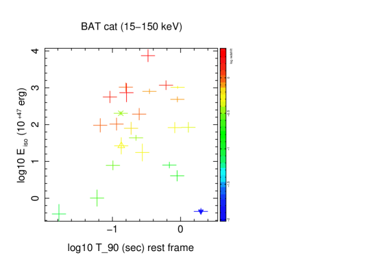
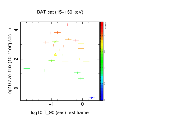
Figure 1: Left: $E_{iso}$ of short GRB’s with known redshift in the Swift-BAT $15-150$ keV energy band. Right: Average flux of the same data. The data is taken from the Swift GRB on-line database https://swift.gsfc.nasa.gov/archive/grb_table/ using as selection criteria $T_{90}\leqslant 2$ sec. Redshift is color coded. As GRB 170817A was not in the FoV of the Swift-BAT, we have used fluence measured in the Fermi-GBM 10 keV-2 MeV band. Thus, $E_{iso}$ and average flux of GRB 170817A shown here are upper limits and shown with an inverse triangle as the symbol of upper limit. Star symbol presents kilonova/GRB 130603B and up-right triangle is GRB 160624A at $z=0.483$, the only GRB with known redshift since 01 September 2015, considered as the beginning of the Advanced LIGO operation, which its GW could be apriori observed if it was at a lower redshift.

3 Analysis and modeling of GW/GRB 170817A data

Observations of thousands of gamma-ray bursts and their afterglows by Swift, Fermi, Konus-wind, and other high energy satellites and ground based robotic telescopes have demonstrated that the main component in the prompt gamma-rays and their afterglows in lower energies is synchrotron emission generated in relativistic or mildly relativistic shocks. In this section we first briefly review a phenomenological shock and synchrotron emission formalism developed in [126, 127]. Then, we use it to analyse both prompt gamma-ray and afterglows of GW/GRB 170817A. A more extensive review of the model can be found in [128]. The advantage of this formalism, despite its simplicity, is that it can be applied to both intern and external shocks, and thereby make it possible to construct a consistent and overall picture about: relativistic ejecta from compact objects such as collapsars, BNS and NS-BH mergers; clarify relations between properties of jets and their progenitors; and characteristics of the environment around progenitors, which influence GRB afterglows.

3.1 Phenomenological formulation of relativistic shocks and synchrotron/self-Compton emission

The phenomenological model of [126, 127] assumes that GRB emissions are synchrotron/self-Compton produced by accelerated charged leptons in a dynamically active region in the head front - wake - of shocks between density shells inside a relativistic jet for prompt and with surrounding material for afterglows in lower energies. In addition to the magnetic field generated by Fermi processes in the active region, an external magnetic field precessing with respect to the jet axis may contribute in the production of synchrotron emission. Origin of this field is not relevant for this simple model. It can be the magnetic field of central object or Poynting flow imprinted into the jet/outflow.

An essential aspect of this model, which distinguishes it from other phenomenological GRB formulations, is the evolution of parameters with time. Moreover, simulation of each burst consists of a few time intervals - regimes - each corresponding to an evolution rule (model) for phenomenological quantities such as fraction of kinetic energy transferred to fields and its variation, variation of the thickness of synchrotron/self-Compton emitting active region, etc. Division of simulated bursts to these intervals allows to change parameters and phenomenological evolution rules which are kept constant during one time interval. Physical motivation for such fine-tuning is the fact that GRB producing shocks are in a highly non-equilibrium and fast varying state. In fact, multiple variation of the slope of afterglows light curves, which presumably are produced by external shocks on the ISM or circumburst material is an evidence that they are not completely uniform and their anisotropies affect the emission. Definition of parameters of the model and phenomenological expressions used for the evolution of active region, which in the framework of the model cannot be calculated from first principles are given in Appendix A.

An important issue, specially when considering the best models for a specific burst, is the fact that parameters of model are not completely independent from each others. For instance, fractions of kinetic energy transferred to induced electric and magnetic fields should depend on the strength of the shock, which in turn is determined by the density difference of colliding shells and their relative Lorentz factor. But there is no simple first principle way to incorporate these dependencies to the model.

Originally, the goal of the shock formalism developed in  [126, 127] was modelling prompt and early afterglow emissions, which are presumably generated by a fast and compact ejecta. For this reason, the model assumes uniform properties for the matter in the colliding shells and treats their evolution self-similarly. In other words, evolution of shocks and their synchrotron emission depend only on time or equivalently distance from the center, rather than to both time and distance as independent variables. Due to these simplifications, the formalism cannot take into account lateral variation of properties in the jet/outflow. However, as suggested in the literature [54, 40, 80, 50, 19] and we give more arguments in its favour in this review, the observed late afterglows of GW/GRB 170817A might have been produced by a continuous flow with a time varying profile of density and Lorentz factor. To take into account these variations we simulate afterglows as being generated by a composite jet with different density and speed for each component. They are simulated separately and can be considered as presenting part of the outflow with corresponding properties. We emphasize that these components are effective presentation of sections of a jet or outflow, which due to the simplicity of the model could not be properly simulated as a single entity. Therefore, it is meaningless to e.g. consider their interaction with each others.

3.2 Prompt emission

The large number of parameters of the model used here does not allow a systematic exploration of the parameter space. To facilitate the search for plausible models for GW/GRB 170817A we use simulations of typical short GRBs in [127] as a departure point and adjust parameters, notably physically most important ones, namely: $r_{0}$, $p$, $\gamma_{cut}$, $\gamma^{\prime}_{0}$, $\Gamma$, $Y_{e}\epsilon_{e}$, $\epsilon_{B}$, $N^{\prime}$, $n^{\prime}_{c}$ and $|B|$ around their prototype values to obtain an acceptable fit to the Fermi-GBM prompt gamma-ray light curve and spectrum. We emphasize that as the exploration of parameter space of the model is not systematic, values of parameters for best models should be considered as order of magnitude estimation.

Giving the unusual characteristics of GRB 170817A, we try 3 range of Lorentz factor to see which one lead to a satisfactory model. Additionally, this exercise allows to explore the well known parameter degeneracy of shock/synchrotron model of gamma-ray bursts. Categories are:

Ultra-relativistic jet with $\Gamma\sim\mathcal{O}(100)$ [122, 123, 28], see also simulations in [127];

Structured relativistic jet with $\Gamma\sim\mathcal{O}(10)$ [115, 92];

Mildly relativistic cocoon with $\Gamma\sim\mathcal{O}(1)$ [86, 85, 54, 40, 56].

Here a cocoon means a mildly relativistic, mildly collimated outflow with a Lorentz factor of $\sim 2-3$. Nonetheless, its angular extension far from the core of the ejecta may have smaller Lorentz factor. This slow part of the outflow is not relevant for the high energy prompt emission but as we show in the next subsection it can be important for the radio afterglow.

Our tests show that a cocoon model cannot reproduce Fermi data. Therefore, we do not discuss such models further in this section. Examples of such models are discussed in [129]. We should also remind that these cocoon models are not exactly the same as cocoon break out model [86] suggested by [40, 87], which is a different mechanism, i.e. not exactly a synchrotron emission. In any case, as we show in Sec. 3.3 a cocoon or cocoon break out or a chocked jet in the cocoon break out alone cannot explain prompt gamma-ray and even afterglows, because X-ray afterglow needs a jet with an ultra-relativistic component.

Fig. 2 shows light curves of 4 simulated bursts with best chi-square fits to the Fermi-GBM’s 10 keV-1 MeV band data. The two peaks in the observed light curve are simulated separately and adjusted in time such that the sum of two peaks minimize the chi-square fit. Fig.3 shows light curves in narrower bands for each peak. Table 1 shows the value of parameters for these simulations. Examples of light curves and spectra of simulations which were explored to find best fits to the data are given in [129] and interested readers can refer to that work. In addition, those simulations were necessary to understand degeneracy of the model and how they might impact interpretation of the results.

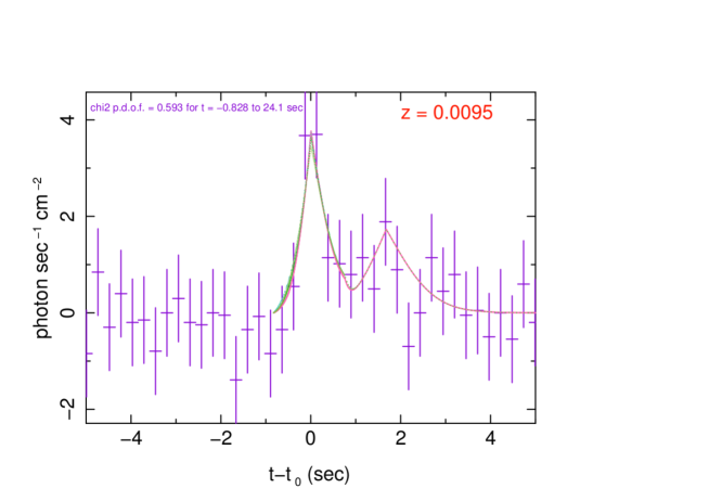
Figure 2: Light curves of 4 best simulations in 10 keV - 1 MeV. The data is from observations of Fermi-GBM [39]. This plot shows that these simulations have very similar light curves. The inset is a zoom on the first peak and shows the slight difference of the amplitude of the first peak in these models. The value of $\chi^{2}$ is for the full line corresponding to model No. 2 in Table 1 for the first peak and model No. 3 for the second peak. Other curves (doted lines) correspond to model No. 1 with and without an external magnetic field (blue and dark green curves, respectively), and an off-axis model with all parameters the same as model No. 2, except column density of ejecta which is $n^{\prime}_{c}=5\times 10^{25}$ cm^-2 (light green). The value of $\chi^{2}$ per degree of freedom of the first two simulations are about $0.02$ larger than model No. 2 and that of the last model is $\sim 0.03$ larger.

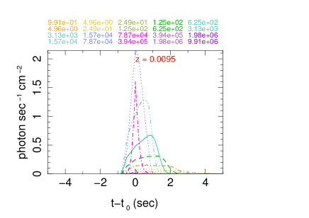
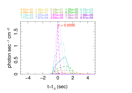
Figure 3: Light curves of simulated models in energy bands covered by Fermi-GBM and Integral SPI-ACS instruments: Left) Simulation No. 2; Center) Simulation No. 1 without external magnetic field; Right) Second peak, that is simulation No. 3. All simulation numbers refer to Table 1. Minimum and maximum of each energy band in eV is written in the corresponding color on the top of each plot. Notice that the second peak is simulated in lower energy bands than the first peak. The lag between highest energy bands is roughly zero and consistent with observation of short GRBs.

Degeneracy of light curve can be partially resolved by fitting the spectrum of the first peak to data, shown in Fig. 4. We do not fit spectrum of the second peak because Fermi spectrum of this peak [39] includes only 2 measured points at lowest energies and the rest are upper limits. It is evident that model d) in Fig. 4 has a weaker fit to data than others. However, in view of uncertainties of the data, their differences are too small to provide a statistically significant criteria in favour of one of these models. Nonetheless, comparison of spectra in 4-a and 4-b, which their only difference is an external magnetic field in the former, may be interpreted as the necessity of a weak magnetic field in addition to the field induced by Fermi processes in the shock front. Indeed, in the next section we show that the remnant of the jet after internal shocks had preserved its collimation and coherence well after prompt shocks. Therefore, it had to have intrinsic magnetic field. As for degeneracies, they can be ultimately removed when the same formalism is used to analyse afterglows of this burst.

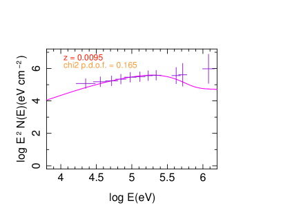
a)	b)
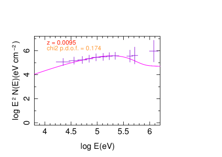
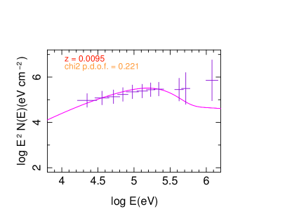
c)	d)

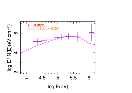
Figure 4: Spectra of simulated models fitted to Fermi-GBM data: a) Model No. 1; b) Model No. 1 without external magnetic field; c) Model No. 2; d) A model with the same parameters as models No. 2 except for $n^{\prime}_{c}=5\times 10^{25}$ cm^-2. As the published spectral data in [39] is in count rate, after changing it to energy flux we used peak energy from [39] to normalize the data such that at $E=E_{peak}=215\pm 54$ keV observed and simulated spectra have the same amplitude. For this reason, spectra of simulated models have much smaller $\chi^{2}$ than their corresponding light curves.

Table 1: Parameter set of simulated prompt emission models

Model Descr.	mod.	$\Gamma$	$r_{0}$ (cm)	$\frac{\Delta r_{0}}{r_{0}}$	$(\frac{r}{r_{0}})_{max}$	$p$	$\gamma_{cut}$	$\kappa$	$\gamma^{\prime}_{0}$	$\tau$	$\delta$
1: GW/GRB 170817: first peak, rel.jet	1	100	$2\times 10^{10}$	$5\times 10^{-5}$	1.5	2.5	10	0	1.5	-	1
	0	-	-	-	1.5	-	10	0	-	0	-
	2	-	-	-	1.5	-	10	0	-	-	3
	2	-	-	-	4	-	10	0	-	-	5
2: GW/GRB 170817: first peak, off-axis	1	10	$2\times 10^{10}$	$5\times 10^{-5}$	1.5	2.5	10	0	1.5	-	1
	0	-	-	-	1.5	-	10	0	-	0	-
	2	-	-	-	1.5	-	10	0	-	-	3
	2	-	-	-	4	-	10	0	-	-	5
3: GW/GRB 170817: second peak	1	30	$6\times 10^{10}$	$5\times 10^{-5}$	1.5	2.5	10	0	1.5	-	1
	0	-	-	-	1.5	-	10	0	-	0	-
	2	-	-	-	1.5	-	10	0	-	-	3
	2	-	-	-	4	-	10	0	-	-	5

Table 1: (continued) Parameter set of simulated prompt emission models

Model Descr.	$\epsilon_{B}$	$\alpha_{B}$	$\epsilon_{e}Y_{e}$	$\alpha_{e}$	$N^{\prime}$ (cm-3)	$n^{\prime}_{c}$ (cm-2)	$|B|$ (kG)	$f$ (Hz)	$\alpha_{x}$	$\phi$(rad.)
1: GW/GRB 170817: first peak, rel.jet	$10^{-4}$	-1	0.01	-1	$2\times 10^{14}$	$10^{25}$	0.8	500	-	-
	-	-2	-	-2	-	-	-	-	1	-
	-	2	-	2	-	-	-	-	2	-
	-	4	-	4	-	-	-	-	3	-
2: GW/GRB 170817: first peak, off-axis	$10^{-4}$	-1	0.03	-1	$2\times 10^{14}$	$5\times 10^{24}$	0.5	500	1	-
	-	-2	-	-2	-	-	-	-	1	-
	-	2	-	2	-	-	-	-	2	-
	-	4	-	4	-	-	-	-	3	-
3: GW/GRB 170817: second peak	$10^{-4}$	-1	0.01	-1	$2\times 10^{13}$	$5\times 10^{23}$	0	-	-	-
	-	-2	-	-2	-	-	-	-	-	-
	-	2	-	2	-	-	-	-	-	-
	-	4	-	4	-	-	-	-	-	-

$\star$ Each data line corresponds to one simulated regime, during which quantities listed here remain constant or evolve dynamically according to fixed rules. A full simulation of a burst usually includes multiple regimes (at least two).

$\star$ Horizontal black lines separate time intervals (regimes) of independent simulations identified by the number shown in the first column.

$\star$ A dash as value for a parameter presents one of the following cases: it is irrelevant for the model; it is evolved from its initial value according to an evolution equations described in [126, 127]; or it is kept constant during all regimes.

Parameters of the best models of the prompt emission show that in comparison with other short GRBs with accompanying kilonova such as GRB 130603B [6, 112] Lorentz factor and densities of colliding shells of GRB 170817 in our direction was at least a few folds smaller, see [129] for details. Although off-axis view of the jet, as we will discuss further in the next subsection, may be somehow responsible for the weakness of this burst, there is evidence for the involvement of intrinsic characteristics. This subject will be more detailed in Sec. 5.

3.3 Late afterglows

As we discussed in Sec. 2 electromagnetic afterglows of GW/GRB 170817A were the most unusual among both short and long GRBs. Notably, long lasting brightening had never been observed in any other GRB. It is however useful to remind that at present no other GRB had follow up observations for as long as this burst. In particular, follow up of other short GRBs have been limited to just a few days. Thus, we ignore how exceptional is the behaviour of afterglows of GW/GRB 170817A.

Although, off-axis view of a structured jet predicts late brightening of afterglows [66, 67, 78, 56], the observed decline of X-ray flux at $\lesssim T+134$ days [19] is inconsistent with simulations of significantly off-axis emission [67], which predict a break after a few hundred days. Other simulations, for instance those reported by [78, 38] predict earlier break, but cannot discriminate between off-axis structured jet and cocoon models [80] and need polarimetry and imaging to discriminate between them [38]. In any case, initially it seemed reasonable to assume that at late times the section of the jet along our line of sight, which even before prompt shocks was not as dense and boosted as in typical short GRBs, had to have dissipated its energy, and its Lorentz factor and density should have been decreased to negligibly small values. In this case the late brightening had to have another origin, for instance MHD instabilities leading to an increase in magnetic energy dissipation [68, 12]; external shock on the ISM/circumburst material of a mildly relativistic thermal cocoon ejected at the same time as the dissipated relativistic GRB making jet [85, 22]; late outflows from an accretion disk [83]; or decay of isotopes in the kilonova [130, 61]. Therefore, it was not certain that late afterglows were directly related to the relativistic jet models concluded from analysis of the prompt emission, see also the commentary of [120] on the issue of finding a reliable explanation for this exceptional discovery.

Here we first discuss simulation of external shocks of a mildly relativistic outflow on the ISM/circum-burst material in the framework of formalism reviewed in Sec. 3.1 and highlight shortcomings of such models for afterglows of GW/GRB 170817A. Then, we discuss models which can explain the data.

3.3.1 Shortcomings of a mildly relativistic outflow

Irrespective of energy dissipation mechanism, most of explanations described in the previous paragraphs predict a mildly relativistic outflow with a Lorentz factor $\Gamma<5$ as the ultimate origin of afterglows. Indeed, even one of the best prompt models shown in Figs. 2 and 4 has a Lorentz factor $\Gamma\sim\mathcal{O}(10)$. Energy dissipation, e.g. through weak internal shocks and interaction with material close to the merger could easily reduce jet’s Lorentz factor to $\Gamma\sim 2-3$, as had been suggested in the early literature on afterglows of GW/GRB 170817A. Fig. 5 shows a few examples of synchrotron emission from external shocks of such outflows. It is clear that none of them can fit all the multi-band data. Although models in Fig. 5-a & b fit well X-ray data, they over-produce both optical and radio emission. By contrast, models c) and d) in this figure have an acceptable fit to radio data, but not enough X-ray and both of them over-produce optical emission by a large amount.

Regarding performance of these simulation, several issues need more clarification. It is well known that synchrotron self-absorption of radio emission can be important. In this case, one can assume that most of radio emission in the model a) which has higher Lorentz factor is absorbed and only radio from a slower and less dense section of outflow, presented by models c) and d), can escape the shocked region. Examples of the effect of self-absorption are presented in [130]. On the other hand, this explanation cannot solve the problem of over-production of optical photons. Although the simulated optical band in Fig. 5 is wider than HST F606W and SDSS r’ filters or equivalents used for acquiring data shown in these plots, it is unlikely that multiple orders of magnitude deviation between these models and data can be due to the wider simulated band. Moreover, it is crucial to remind that optical data is dominated by kilonova mission, which has very different origin and spectrum. Therefore, the optical data must be considered as an upper limit to any contribution from the GRB. This makes models shown in Fig. 5 even more distant from data, unless optical photons is strongly observed. Alternatively, one can make simulations consistent with optical data, but an additional source of X-ray would be necessary to explain these observations.

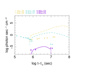
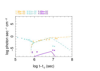
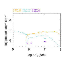
a)	b)	c)	d)

Figure 5: X-ray, optical, and radio light curves of simulated models without taking into account synchrotron self-absorption. Stars present data taken from: [78, 88] (X-ray), [108, 92, 75, 19] (optical), [1, 47, 27] (radio). Model a) has $\Gamma=2.3$ and others have $\Gamma=1.2$. Complete list of parameters for these simulations can be found in [130]. If it is assumed that the centroid of outflow is oblique with respect to the line of sight, the effect of projection must be taken into account and the Lorentz factor should be considered to be larger by a factor of $1/\cos\theta_{c}$, where $\theta_{c}$ is the angle between centroid of outflow and the line of sight.

The outline of this exercise is that the assumption about extreme energy dissipation in the jet after prompt emission is not realistic. Indeed, to increase the contribution of X-ray emission and decrease the number of soft photons the spectrum of synchrotron emission must be harder, i.e. its peak must be pushed to higher energies such that low energy emissions fall on the fast declining side of the spectrum, see examples of synchrotron/self-Compton spectra of GRBs in [127, 128]. On the other hand, realization of this requirement needs larger Lorentz factors. Moreover, the fact that combination of two simulations gives a better fit to data than each component alone reminds us that the formulation of [126] assumes a jet with uniform Lorentz factor and density. But numerical simulations of ejecta from BNS [34, 57, 49, 24, 24] and its further acceleration by transfer of Poynting to kinetic energy [60] shows that both these processes are inhomogeneous. Consequently, the final relativistic jet has a profile with varying $\Gamma$, density and extension. Another crucial property of emissions from a relativistic jet is their beaming for a far observer. Due to this relativistic effect only an angle $\theta_{max}=\arcsin(1/\Gamma)$ around the line of sight is visible to the observer. As we discussed in Sec. 3.2 at the time of prompt emission the jet is ultra-relativistic and $\Gamma\gtrsim\mathcal{O}(100)$. Therefore, beaming allows to see only emission from a small part of the jet along the line of sight. Consequently, anisotropy of the jet is not visible, specially when only a relatively narrow gamma-ray band is observed. By contrast, afterglows are usually observed in broad bands - from gamma and X-rays to radio - and low energy emissions from side lobes - high latitudes - of the jet would be visible and important.

3.3.2 Multi-component models

The shortcoming of models simulated in [126, 127] can be compensated by constructing multi-component models in which each component presents approximately an angular section of the jet profile with different Lorentz factor, density and extension. In addition, as argued in the previous subsection, we allow the presence of an ultra-relativistic component. This strategy, leads to a model and a few of its variants which fit X-ray and optical data well and satisfy the upper limit constraint imposed by observed optical data [131]. Parameters of the components of the model are shown in Table 2. Fig. 6 shows light curves of components of this model and their sum in each band. As this model and some of its variants shown in Fig. 8 fit well radio and X-ray data, we presume that their predictions for optical emission of the GRB afterglow should be reliable. Under this assumption, these models show that after $\sim T+200$ days kilonova emission in optical/IR bands was not anymore significant and the afterglow was dominated by synchrotron emission from external shocks of the relativistic polar outflow from the merger.

Spectra of the components and total spectrum of the model are shown in Fig. 7. They show a good consistency between simulated spectrum and the data, and as expected, amplitude of optical emission at $\sim T+\mathcal{O}(10)$ days is higher than the afterglow model. Moreover, due to the dominance of kilonova contribution, the shape of pseudo-spectrum of energy flux shown in Fig. 4-b at this epoch is significantly different from those of later times. In addition, Fig. 4-c shows a crude broad-band spectral slope, which is determined from radio and X-ray data only and thereby is not contaminated by kilonova emission. Ignoring large uncertainties of calculated slopes, they show a behaviour similar to other GRB afterglows, namely softer spectrum during earliest observations around $T+\mathcal{O}(10)$ days, which gradually becomes harder until the peak of emissions around $T+110$ days, and finally softens at later times. Therefore, despite unusual brightening of afterglows, they have the same spectral trend as other GRBs.

a)	b)

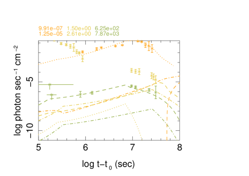
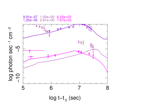
Figure 6: a): Radio, optical/IR, and X-ray light curves of simulated 3-component. Left: Light curves of the 3 components: ultra-relativistic (C1) (dash lines), relativistic (C2) (dash-dot), mildly relativistic (C3) (dotted lines). The energy range for each band is written on the top of each plot in the same colour/gray scale as the curves. Stars present data taken from: [78, 88, 116, 45] (X-ray), [108, 92, 75, 19, 97, 65] (optical), [1, 47, 27, 82] (radio). The upper limit of X-ray flux at $<T+10$ is from Neil Gehrels Swift-XRT [29] and the upper limit at $\sim T+2.2$ is from Chandra observations [115]. b): Sum of the light curves of the 3 components: radio (magenta/light grey), optical (purple/medium grey), X-ray (dark purple/dark grey).

a)	b)	c)

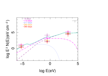
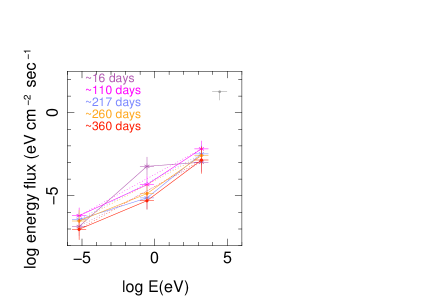
Figure 7: a): Spectra of components and their sum: ultra-relativistic (C1) (dash line), relativistic (C2) (dash-dot), mildly relativistic (C3) (dotted line), sum of 3 components (full line). Crosses present observations at different times in radio, optical/IR, and X-ray, optical and radio bands. When data for a time interval was not available an interpolation has been used. The width of crosses presents the width of the corresponding filter and are much larger than observational uncertainties. The upper limit at $E\sim 16-50$ keV is from the Swift-BAT survey data [63]. To generate a pseudo-spectrum from flux measurements, we have normalized data such that X-ray at $T+217$ days become equal to maximum of simulated spectrum in the simulated energy interval. b): Spectrum of energy flux. The lines connecting the data points are added to facilitate the illustration of spectral variation. c): Evolution of the slope of pseudo-spectrum using only radio and X-ray data, that is slope of dotted lines in b). The shaded region is the estimate of uncertainty of calculated slopes according to variation rule.

Table 2: Parameter set of simulated afterglow components.

Comp.	mod.	$\gamma^{\prime}_{0}$	$r_{0}$ (cm)	$\frac{\Delta r_{0}}{r_{0}}$	$(\frac{r}{r_{0}})_{max}$	$p$	$\gamma_{cut}$	$\kappa$	$\delta$	$\epsilon_{B}$	$\alpha_{B}$	$\epsilon_{e}Y_{e}$	$\alpha_{e}$	$N^{\prime}$ (cm-3)	$n^{\prime}_{c}$ (cm-2)
Ultra. rel. (C1)	1	130	$10^{16}$	$10^{-7}$	1.5	1.8	100	-0.5	0.5	$0.08$	-1	0.1	-1	$0.04$	$5\times 10^{22}$
	2	-	-	-	15	-	100	0.3	0.1	-	0	-	0	-	-
	2	-	-	-	20	-	100	0.4	0.05	-	1	-	1	-	-
Rel. (C2)	1	5	$10^{16}$	$10^{-6}$	2	2.1	100	-0.5	1	$0.08$	-1	0.1	-1	$0.04$	$10^{23}$
	2	-	-	-	40	-	100	0.4	0.1	-	0	-	0	-	-
	2	-	-	-	100	-	100	0.5	1	-	1	-	1	-	-
Mildly rel. (C3)	1	1.06	$1.5\times 10^{16}$	$10^{-2}$	1.5	1.8	100	-0.5	1	$0.08$	-1	0.02	-1	$0.008$	$10^{24}$
	2	-	-	-	10	-	100	0.	0.1	-	0	-	0	-	-
	2	-	-	-	10	-	100	1	1	-	1	-	1	-	-

$\star$ Each data line corresponds to one simulated regime, during which quantities listed here remain constant or evolve dynamically according to fixed rules. A full simulation of a burst usually includes multiple regimes (at least two).

$\star$ Horizontal black lines separate time intervals (regimes) of independent simulations identified by the label shown in the first column.

$\star$ A dash as value for a parameter presents one of the following cases: it is irrelevant for the model; it is evolved from its initial value according to an evolution equations described in [126, 127]; it is kept constant during all regimes.

3.3.3 Degeneracies

Despite the fact that the model described in Table 2 provides a good fit to the data, some issues should be considered before making any conclusion. Notably, as we explained in Sec. 3.1 parameters of the phenomenological formalism of [126, 127] are not completely independent, and thereby they may be degenerate. Thus, before interpreting this model and concluding properties of the jet from it, we must consider implications of these degeneracies. For this purpose, change of the characteristics of the model as a function of their variation is studied in some extent in [131]. Here we summarize them by showing in Fig. 8 a few variants for components of the model which can fit the data as good as those presented in Table 2. Specifically, Fig. 8-a shows an alternative to component C1 with smaller ISM/circum-burst density but longer jet extent. It fits X-ray data as good as C1 in Table 2, but future observations should be able to distinguish between them.

Variant of C3 shown in Fig. 8-b is important because it has a Lorentz factor consistent with superluminal motion of radio counterpart [81, 37]. Alternatively, with slight modification of column densities and/or thicknesses of active regions $\Delta r$ in these models we can consider both of them as components of the full model. Indeed, evidence for a mildly relativistic component with small Lorentz factor - a cocoon - is observed in long GRB 171205A and its associated supernova SN2017uk [52], and has $\beta\sim 0.3$, corresponding to $\Gamma\sim 1.05$, i.e. similar to C3 component in Table 2. Therefore, model C3 and its variant in Fig. 8-b may present sectors further and closer to the jet axis, respectively.

Another important conclusion from the study of parameter degeneracy is the influence of distance between merger and location of external shocks on the slope of the light curve and time of its turnover. See [131] for example of models with shorter distances than $\sim 10^{16}$ cm used in the model of Table 2. The peak light curves in these models are too early and inconsistent with the data.

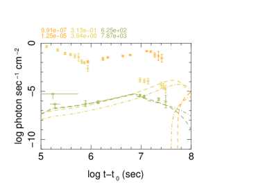
a)	b)
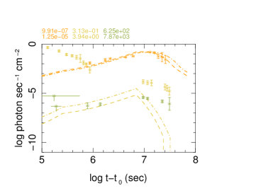
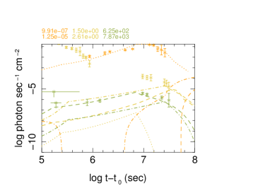
c)	d)

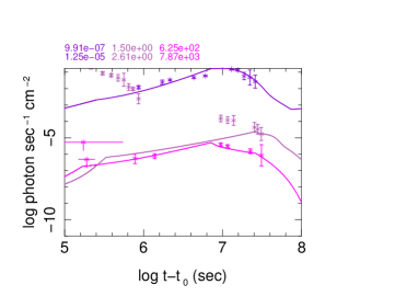
Figure 8: Variants of components of the model of Table 2 which fit the data: a) A variant of component C1 with $\Delta r_{0}/r_{0}=10^{-6}$, $N^{\prime}=0.004$ cm^-3 (dash-dot); b) A variant of C3 with $\gamma^{\prime}_{0}=\Gamma=4$, $r_{0}=10^{16}$ cm, $\Delta r_{0}/r_{0}=10^{-3}$, $N^{\prime}=0.001$ cm^-3, $n^{\prime}_{c}=10^{25}$ cm^-2 (dash-dot); c) Variant of C2 component with $\gamma^{\prime}_{0}=\Gamma=30$, $\Delta r_{0}/r_{0}=10^{-5}$, $n^{\prime}_{c}=10^{22}$ cm^-2, $N^{\prime}=0.008$ cm^-3 (dash-dot); In all these plots dashed lines correspond to the components described in Table Table 2; d) Total light curves for a model with C1 and C2 as in Table 2 and C2 as shown in c).

3.4 Other models and their consistency with data

In our knowledge [129] is the only detailed modeling and analysis of the prompt gamma-ray emission of GW/GRB 170817A. Therefore, here we only compare afterglow models described in Sec. 3.3 with some of the proposed models in the literature.

Fitting afterglow data with a multi-component model in [131] is not unique and some other authors have similarly modelled late afterglows of GW/GRB 170817A in this manner. For instance, [78, 2] consider a two component structured jet model with a top-hat ultra-relativistic component and $\Gamma\sim 100$ in its inner $\theta\lesssim 9^{\circ}$, where $\theta$ is angle with respect to symmetry axis of the outflow, and a component with a decreasing Lorentz factor in the angular interval $10^{\circ}\lesssim\theta\lesssim 60^{\circ}$ with a mean $\Gamma\sim 10$. They use a relativistic jet simulation code to find that a line of sight angle from the jet axis $\theta_{v}\sim 20^{\circ}$. This model is very similar to the model described in the latest version of [67], but Lorentz factor and energy profile of the jet in the two works are different. Authors of [84] also conclude an initially ultra-relativistic jet from their analysis of afterglows. Authors of [65] consider two profiles for the jet, one similar to 2-component model of [78, 2] and the other with Gaussian energy and Lorentz factor profiles. Both models find a small central core opening angle of $\lesssim 5^{\circ}$. In their 2-component model high and low Lorentz factors are $\sim 100$ and $\sim 5$, respectively. However, in the Gaussian model on-axis Lorentz factor can be as large as $900$. A phenomenological function which effectively has two coupled components is used by [82].

It should be pointed out that asymptotic formulation of synchrotron emission from external shock formulation in [100], which is used in all the cited works, considers a uniform spherical ejecta. Therefore, conclusions about viewing angle of the jet in the cited works is based on the value of Lorentz factor and beaming of emissions from a relativistic source [98]. An interpretation of the multi-component model of Table 2 in the framework of [100] formulation can be found in [131].

4 Interpretation of models

In this section we use models of prompt and afterglows described in the previous section to check their consistency, remove degeneracies, and correlate them to properties of progenitor neutron stars, their environment and merger, and its ejecta.

4.1 Selecting between prompt models

Although simulations of prompt gamma-ray emission show that both an ultra-relativistic jet with a Lorentz factor of $\mathcal{O}(100)$ and a relativistic jet with a Lorentz factor of $\mathcal{O}(10)$ are consistent with data, afterglows rule out the latter case. We should remind that the analysis of prompt gamma-ray emission in [129] was performed well before the relatively early turn over of afterglows. Therefore, they could not be used to distinguish between the two possible range of initial Lorentz factor, which might additionally discriminate between a significantly off-axis view of the jet and otherwise. For this reason, in [129] several other arguments were given in favour of an ultra-relativistic jet with $\Gamma\sim\mathcal{O}(100)$. Here we briefly review them because this approach may be useful for analysing future GW/GRB events.

Giving relation between emitted and received power from a relativistic source $(dP_{e}/d\omega d\Omega)/(dP_{r}/d\omega d\Omega)=1/\Gamma^{2}(1+\beta\cos\theta_{v})$, it is clear that off-axis view alone cannot explain intrinsic faintness of the burst, if the jet is uniform. Therefore, GW/GRB 170817 had to have a structured jet. On the other hand, even during prompt internal shocks energy dissipation significantly reduces Lorentz factor, see Fig. 9, and scattering of particles by induced electromagnetic fields generates a lateral expansion. This process should bring dissipated material and its emission to the line of sight [66] and should have been detectable as a tail emission, which is detected in some short bursts, and/or it should have generated bright early afterglows. None of these emissions are observed in GW/GRB 170817A event. Thus, according to this argument even an off-axis view of a structured jet cannot explain the faintness of the prompt gamma-ray and early afterglows and their late and slow brightening.

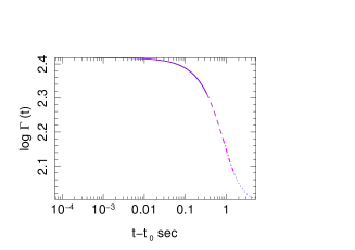
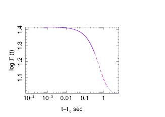
Figure 9: Evolution of Lorentz factor of the fast shell with respect to a far observer at the redshift of the source during internal shocks. Left: ultra-relativistic jet (Model 1 in Table 1); Right: relativistic jet (Model 2 in Table 1). Different line styles present simulation regimes.

Another criteria for choosing between low and high Lorentz factor candidate models of Table 1 is plausibility of parameters which characterize shocks and synchrotron emission. Table 1 shows that in the moderately relativistic Model 2 smaller Lorentz factor is compensated by a higher fraction of energy transferred to electrons (more generally charged leptons), which is $\sim 3$ times larger than in the ultra-relativistic jet Model 1. However, apriori due to the low density of the jet in this model interaction between charged particles and their scattering had to be rarer and induced electric and magnetic fields weaker. Moreover, low electron yield of neutron rich BNS ejecta [96, 58, 57] should have made the transfer of kinetic energy to electrons even harder. Estimation of electron yield $Y_{e}$ for various components of the ejecta of GW 170817 event based on the observation of r-process products [49, 103] are: $Y_{e}\sim 0.1-0.4$ for dynamical component, $Y_{e}\sim 0.3$ for wind, and $Y_{e}\sim 0.25$ in another wind component [92]. Considering the value of $\epsilon_{e}Y_{e}$ in the low Lorentz factor Model 2, the effective fraction of kinetic energy transferred to electrons had to be $\epsilon_{e}\sim 0.1-0.3$, which is much higher than $\epsilon_{e}\lesssim 0.1$ found in Particle In Cell (PIC) simulations [109, 104, 105]. By contrast $\epsilon_{e}$ of Model 1 is comfortably in the PIC range.

In conclusion, Model 1 seems more plausible than Model 2. Considering parameters of Model 1 as approximately presenting properties of the jet before prompt internal shocks, according to simulations of [127] its bulk Lorentz factor in our direction was a few folds smaller than typical short bursts. Additionally, densities of colliding shells were more than one order of magnitude less brighter GRBs. Moreover, these findings demonstrate that most probably in addition to off-axis, intrinsic properties of progenitor neutron stars and dynamics of their merger and ejecta were responsible for the faintness of GRB 170817A. In addition, the lack of bright short GRBs at low redshifts in Fig. 1 is an evidence for the influence of progenitor BNS evolution on the strength of GRBs produced during their merge.

4.2 Kinematic of the jet at late times

The structure of 3-component jet model at late times, that is $>T+10$ days, discussed in Sec. 3.3 is in agreement with our arguments in favour of an ultra-relativistic prompt jet with a Lorentz factor $\Gamma\sim 100$ at the end of internal shocks. As discussed earlier, exploration of the parameter space of external shocks in [130, 131] to find a model with only relativistic or mildly relativistic Lorentz factor was not successful. Apriori Lorentz factor of the jet at the location of external shocks $r_{e}$ should be smaller than its value at the end of internal shocks at $r_{i}$ because weaker internal shocks and cooling of shocked material should reduce its kinetic energy. Therefore, the presence of an ultra-relativistic component with roughly the same Lorentz factor in the afterglow model means that despite all odds, a fraction of ultra-relativistic jet had survived up to long distances. However, comparison of the column density of the prompt jet in Table 1 with that of component C1 in Table 2 show that its column density at the time of external shocks was reduced by a factor of $\sim 200$. If the jet were an adiabatically expanding cone, its column density had to decline by a factor of $(r_{i}/r_{e})^{-2}\sim 10^{12}$. The much smaller dilation factor according to models described here means that the material inside the jet had an internal coherence and collimation - most probably through imprinted electric and magnetic fields in the plasma. Thus, we conclude that its geometry and expansion were closer to a boosted cylinder rather than an adiabatic cone. In addition, in [131] it is shown that non-adiabatic expansion of jet cannot be associate to accretion of material, which could completely extinguish its boost.

4.2.1 Late time jet structure and interpretation of components

As discussed earlier, unusual characteristics of GRB 170817A may be in some extent due to the off-axis view of the jet. Indeed, observation of gravitational waves from this transient indicates an orbital inclination angle of $18^{\circ}\lesssim\theta_{in}\lesssim 27^{\circ}$ [76]. Moreover, superluminal motion of radio afterglow with an apparent speed of $\beta_{app}=4.1\pm 0.5$ [81, 37] is evidence of an oblique view of its source.

Due to relativistic beaming of photons, off-axis view of the jet has significant consequences for observations. A far observer receives synchrotron emission only from a cone with half angle $\theta_{max}\equiv\arcsin(1/\Gamma)$ with respect to the line of sight. For components C1, C2, and C3 of the afterglow model listed in Table 2 these angles are $\theta_{max_{1}}\sim 0.5^{\circ}$, $\theta_{max_{2}}\sim 11.5^{\circ}$ and $\theta_{max_{3}}\sim 65^{\circ}$ or $14.5^{\circ}$ for C3 in Table 2 and the model in Fig. 8-b as its alternative or an additional component, respectively. This leads us to conclude that the 3 (or 4)-component model of the jet at the time of external shocks presents a structured jet and components of the model approximately present its angular structure and characteristics of its shock on the surrounding material from our line of sight up to its outer boundary. In particular, their Lorentz factors and column densities present azimuthal variation of material load of the polar outflow and its velocity up to a $\cos\theta$ factor, that is $\Gamma_{simul,i}=\Gamma_{i}(\theta_{i})\cos\theta_{i}$, where $\theta_{i}$ is angle between centroid of component $i$ of the model and the line of sight.

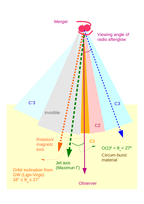
Figure 10: Schematic description of polar outflow of merger at the time of its encounter with circum-burst material. C1, C2, C3 refer to components of the simulated model. Grey shaded region on the opposite side of the jet with respect to observer’s line of sight is approximately invisible because of its large Lorentz factor and off-axis angle. Nonetheless, C’3 region which has even larger off-axis may be visible if its Lorentz factor is sufficiently low. Therefore, there can be a contribution to component C3 of the model from emission of this region. In any case, due to its large off-axis contribution of C3’ would be subdominant. For the sake of simplicity here we have assumed that magnetic field direction and rotation axis coincide. This may not be true.

Fig. 10 shows a schematic presentation of this interpretation, components of the model, and their positions with respect to our line of sight. We remind that jet axis may be inclined with respect to rotation axis of the merger [60]. Considering this possibility and estimated inclination of orbit, viewing angle is constraint to $\mathcal{O}(1^{\circ})\lesssim\theta_{v}\lesssim 27^{\circ}$. This is consistent with estimations of [78, 2, 81], but not very restrictive. Moreover, it does not provide any information about Lorentz factor of the invisible core of the jet. Additionally, the maximum off-axis of components according to their Lorentz factor does not fix their centroid. To estimate these quantities we assume a Gaussian profile for the jet and apply constraints on the centroid angles and on the parameters of the profile, see [131] for details. From this analytical approximation we find: $\theta_{2}\sim 9^{\circ}-11^{\circ}$, $\theta_{3}\sim 12^{\circ}-15^{\circ}$, assuming on-axis Lorentz factor $\Gamma_{max}<1000$. In [131] it is shown that the range of allowed values for the viewing angle $\theta_{v}$ is strongly correlated with $\Gamma_{max}$ and is restricted to $5^{\circ}\lesssim\theta_{v}\lesssim 7^{\circ}$ for $\Gamma_{max}\sim 250$ and to $14^{\circ}\lesssim\theta_{v}\lesssim 18^{\circ}$ for $\Gamma_{max}\sim 1000$. For alternative C3 model in Fig. 8-b the range of allowed angles is even more restricted: $\theta_{v}\sim 7.5^{\circ}-8^{\circ}$, for $\Gamma_{max}\sim 250$ and $\theta_{v}\sim 8^{\circ}-15^{\circ}$, for $\Gamma_{max}\lesssim 1000$, and $\theta_{2}\sim 10.5^{\circ}$, $\theta_{3}\sim 11.5^{\circ}$, for any standard deviation of the Gaussian profile as long as $\Gamma_{max}<1000$. Marginalizing over other parameters, the angle between jet axis and rotation axis is constraint to $\sim[7^{\circ}-15^{\circ}]$. An exponential profile does not lead to acceptable values for the parameters and is ruled out.

Although above constraints are more restrictive than those only based on the orbit inclination, due to degeneracies in the parameter space it is still impossible to judge whether the core of the jet had a typical Lorentz factor of $\sim 500$ [127] or had a smaller boost. The latter case means that off-axis viewing angle was only partially responsible for unusual properties of GRB 170817A. We remind that the probability of viewing a jet exactly on axis is very small and a deviation is always expected. Moreover, prompt gamma-ray emission of GRB 170817A is somehow similar to dark short bursts - those without an X-ray counterpart at $\lesssim T+\mathcal{O}(10)$ ksec, see Fig. 11. Although some of these GRB candidates may be faint flares from Soft Gamma-ray Repeaters (SGR) in nearby galaxies, others - specially those with longer $T_{90}$ - might be related to BNS mergers similar to GW/GRB 170817A and two other BNS merger gravitational wave candidate events Ligo/Virgo 190425z and Ligo/Virgo 190510g at redshift $z\sim 0.06$ and $z\sim 0.05$, respectively. For latter events, which were about 6 times further than GW/GRB 170817A only upper limits on any electromagnetic emission is available. Additionally, the host of the faint X-ray dark short GRB 080121 [18] may belong to a galaxy group at redshift $z=0.046$ [91]. If true, this burst was intrinsically only 2 times brighter than GRB 170817A, which its $E_{iso}$ was a few orders of magnitude fainter than typical short bursts, see Fig. 1.

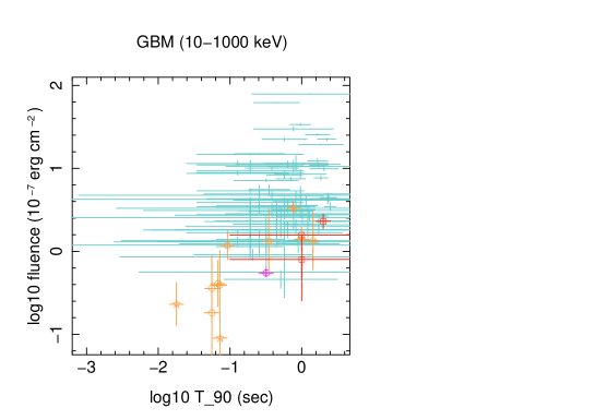
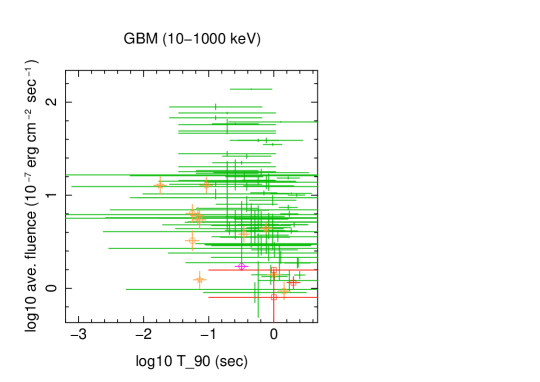
Figure 11: Fluence and flux of nearby Swift short GRBs, GW-BNS events and Swift X-ray dark short GRBs. Left: Fluence in $15-350$ keV band; Right: Average flux. Symbols: Nearby $z<0.2$ short GRBs (star), X-ray dark (circle), GW events (square), Fermi-GBM short GRBs (data without symbol). GRB 080121 is distinguished by its color/grey level from other X-ray dark GRBs. For Ligo/Virgo 190425z and Ligo/Virgo 190510g only upper limit on gamma-ray is available and a $T_{90}=1$ sec is used to calculate average flux.

The faintness or absence of GRB in gravitation wave events associated to BNS may be interpreted as a natural consequence of jets directionality. However, it does not explain the absence of optical emission from ejected disk/torus, which its emission is roughly spherical - presumably due to its faintness. Therefore, despite the impact of off-axis view of GW/GRB 170817A, intrinsic properties of the progenitor BNS, in particular magnetic field of neutron stars, their spin, and their age, might have been involved in its weakness. In [129] this subject is discussed in detail and we summarize its conclusions in Sec. 5.

4.2.2 Delayed brightening

In the literature, along with its intrinsic faintness, the late brightening of GW/GRB 170817A afterglows is usually considered as an exceptional characteristic of this bursts.

Afterglows of GRBs up to few thousands of seconds are most probably a superposition of weak internal shocks in what remains from the relativistic jet after the main prompt shock, and emission from external shocks [121]. Assuming a narrow prompt spike, the delay between the prompt and onset of afterglow emission is $\Delta t\sim r_{e}/2c\Gamma^{2}$, where $c$ is the speed of light. For the model of Table 2 $\Delta t\sim 4$ sec. This delay is much shorter than any automatic follow up and practically unobservable. Thus, the shape of X-ray light curve depends on relative importance of decreasing emission from internal shocks and increasing emission from external shocks. The absence of early brightening or even a plateau in many short GRBs means that their early X-ray is dominated by what we call tail emission of internal shocks. Thus, as pointed out earlier, in absence of long follow up observation of short GRBs we do not usually detect the second component and ignore how its light curve look like at late times. Short GRB’s with a plateau in their X-ray light curve may be those in which the afterglow takes off quickly and peaks a few days after prompt gamma-ray.

The initial suggestions about brightening of afterglows due to the reduction of off-axis view when the jet become dissipated and its content scatter to our line of sight, is not consistent with relatively early break of light curves in all three energy bands after $\sim T+110$ days. Therefore, viewing angle cannot be the only reason for the late brightening of afterglows. On the other hand, our simulations show that in the case of GW/GRB170817A the slow rise of the afterglow was due to the long distance of ISM/circum-burst material from center, its low density and low column density of the jet. Dilution of the jet was partially due to the intrinsically low density and low Lorentz factor of polar ejecta - at least in our direction - and partially the result of large distance of surrounding material from center, that is $\sim 1000$ AU (see Table 2) rather than e.g. $\sim 200$ AU for recently detected NIR emitting material around the isolated neutron star RXJ0806.4-4123 [94]. Consequently, jet’s column density was extensively reduced by lateral expansion.

It is however cautious to consider that our conclusion about the effect of distance may be somehow biased and correlated to spatial resolution of our simulations. Nonetheless, estimation of shock distance for this GRB in the literature and for other GRBs with various methods, such as cooling of thermal emission [89] show that the range of distances obtained from simulation of GRBs by the formalism used here [127] are realistic.

5 Properties of GW/GRB 170817 progenitors and their environment

If the unusual properties of GW/GRB 170817A and presumed faintness of other nearby candidate BNS mergers are merely due to an off-axis view, they tell little about properties of their progenitor neutron stars. By contrast, if the faintness is at least in some extent intrinsic, it may be an evidence for evolution of BNS population. Assuming an intrinsic origin, in this section we use results of GRMHD simulations of BNS merger and observed properties of neutron stars and pulsar, which present a relatively young population with an age less than $\mathcal{O}(1)$ Myr, to understand properties of the nearby, i.e. $z\lesssim 0.1$ BNS and their merger.

5.1 Equation of state, magnetic field and spin

In addition to the relation between mass and radius, the Equation of State (EoS) of neutron stars determines core and crust density and buoyancy, and thereby their tidal deformability [35] which affects high frequency ringdown of gravitational waves at the end of binary’s inspiral. Although resolution of LIGO-Virgo at high frequency is not sufficient for detailed discrimination between equations of states, it is sufficient for distinguishing between stiff, that is high pressure, and soft EoS. In the case of GW 170817 stiff equations of state are disfavored [70]. For close mass NS progenitors - as it was the case of GW 170817 - the density of inner part of the accretion disk and poloidal magnetic field of the merger are smaller in soft EoS [57, 110, 10].

Simulations of [57] show that in equal mass BNS merger, if the initial magnetic fields of progenitors are aligned with each other and anti-aligned with the rotation axis of the BNS, average poloidal magnetic field of the polar ejecta is about 5 times weaker than when both initial fields are aligned with the rotation axis. Additionally, if the initial fields are anti-aligned with each other, the average poloidal field is even smaller by a factor of few. Anti-alignment may happen through interaction of magnetized material surrounding progenitors before the last stages of inspiral. In this case, reduction of the field further from rotation axis is larger. These characteristics have direct impact on attainable Lorentz factor when ejected polar material is accelerated by transfer of magnetic to kinetic energy [60]. On the other hand, star population of the host galaxy NGC 4993 is relatively old [8, 51, 4]. Therefore, magnetic fields of the progenitor neutron stars of GW 170817 might have been as low as $10^{8}-10^{9}$ G and fast precessing, if the progenitors were recycled millisecond pulsars or even smaller if they had evolved in isolation [48, 62].

Initial spins of progenitor neutron stars, which carry a fingerprint of their evolution history, have a crucial role in the dynamics of their merging. In particular, they affect the amount of ejecta, density and extent of accretion disk/torus, and spin of the short living High Mass Neutron Star (HMNS) and the final black hole. Unfortunately, GW 170817 event was too faint and spin of progenitors could not be determined from gravitational waves.

When spin axes are aligned with orbital rotation, binding energy of BNS is weaker, inspiral regime is longer and amount of ejected mass is larger too. However, the latter depends on the mass ratio of progenitors and is smaller for equal mass binaries [9]. It is clear that direction of these differences are similar to those of magnetic field. However, spin effect on the amount of ejected material is subdominant with respect to other processes and can modify it by only a few percents [9].

In summary, the observed properties of GW and electromagnetic emissions of GW 170817 event are consistent with each others and point to a reduced ejecta and magnetic field, and thereby a weak GRB.

5.2 Environment of progenitor BNS

The afterglow model described in Sec. 3.3 requires that density of external material depend on the azimuthal angle with respect to jet axis. Despite degeneracy of the parameters, the directional anisotropy of ISM/circum-burst material may be real because we could not find consistent model without it. This means that circum-burst material was not only the ISM. Moreover, origin of additional material and its properties were somehow correlated with progenitors.

In young neutron stars and pulsars the distance to wind Termination Shock (TS) $R_{TS}$ depends on the rate of mass loss and wind pressure inside wind nebular, which is balanced by the ISM pressure, and its typical value is $R_{TS}\sim\mathcal{O}(0.1)$ pc $\sim\mathcal{O}(10^{17})$ cm  [106]. In old neutrons it is expected that the reduction of glitching activities due to the solidification of crust and dissipation of magnetic field gradually decreases mass loss and $R_{TS}$. However, detection of this population is very difficult and information about their properties is extremely rare. An exception is the isolated neutron star RXJ0806.4-4123 with an age of $\sim 10$ Myr for which thermal material at a relatively short distance of $\sim 200$ AU$~{}\sim 3\times 10^{15}$ cm is detected [94].

Our simulations of the afterglows estimates $R_{TS}\sim 10^{16}$ cm, which is between the above values. The reason may be an age larger than most observed neutron stars and pulsars, estimated to be $\lesssim\mathcal{O}(10^{4})$ yr, and younger than $\sim 10$ Myr age of RXJ0806.4-4123. It is also plausible that the progenitor neutron stars were even older, but during early stages of inspiral, that is well before generation of detectable gravitational waves, strong tidal forces had induced crustal faults and resumed glitching and mass loss. If this explanation is correct, ejected material had to also persist at shorter distances and inside the wind bubble. To estimate their average column density we employ distribution used in the afterglow model for ISM/circum-burst material, that is $N^{\prime}(r)=N^{\prime}(r_{0})(r/r_{0})^{-\kappa}$ and extend it to $r<r_{0}$. For model C1 this estimation gives a column density of $\sim 4\times 10^{14}$ cm^-2, which is much smaller than column density of the components of model. It is also smaller than swept material in the first $\sim 3\times 10^{5}$ sec after the onset of the external shocks, and therefore completely negligible. On the other hand, if we consider much denser circum-burst material at shorter distances, much higher X-ray flux generated by the shocks violates upper limits at $\sim T+2$ days, see additional simulations in [131]. Using these two extreme cases, we conclude that the column density of material inside $r_{e}\sim 10^{16}$ cm bubble was $<\mathcal{O}(1)\times 10^{15}$ cm^-2 or equivalently its average density was $<0.4$ cm^-3.

6 Outline and prospectives for future

In summary, from analysis of prompt and afterglows of GW/GRB170817A along with information acquired from gravitational wave observation we can draw the following consistent picture for the first BNS merger event extensively followed up in multi-wavelength by multi-probe instruments:

- Progenitors were old and cool neutron stars with close masses;

- They had soft equations of state and small initial magnetic fields of $\lesssim 10^{9}$ G. Their fields were anti-aligned with respect to orbital rotation axis and each other.

- For dynamical and/or historical reasons such as encounter with similar mass objects, their spins before final inspiral were anti-aligned.

- The merger produced a HMNS with a moderate magnetic field of $\lesssim 10^{10}$ G. This value is in the lowest limit of what is obtained in typical GRMHD simulations.

- The HMNS eventually collapsed to a black hole and created a moderately magnetized disk/torus and a low density, low magnetized outflow.

- A total amount of $\sim 0.03-0.05~{}M_{\odot}$ material, including $10^{-3}-10^{-2}~{}M_{\odot}$ of tidally stripped pre-merger and a post-merger wind were ejected to high latitudes. They were subsequently collimated and accelerated by transfer of Poynting to kinetic energy. The same process increased electron yield by segregation of charged particles.

- A small mass fraction of the polar ejecta was accelerated to ultra-relativistic velocities and made a relatively weak GRB. The reason for low Lorentz factor, density, and extent of this component was the weakness of the magnetic field.

- For the same reasons, the ultra-relativistic section of the jet was narrow and our off-axis view of $\sim 10^{\circ}$ was enough to reduce the emission of high energy photons in our direction.

- After prompt internal shocks the jet had a wide angular distribution with varying density and Lorentz factor. But despite significant energy dissipation in its core, a tiny fraction of the jet had preserved its coherence and boost up to its collision with circum-burst material at $\sim 10^{16}$ cm from merger.

- In addition to the ISM, circum-burst material included a component which its origin was correlated with the BNS.

- The late brightening of afterglows was due to the relatively long distance of circum-burst material and low density of material inside the wind bubble surrounding the BNS.

- Angular variation in the jet was also responsible for domination of emission in lower energies from high latitude side lobes and thereby observation of a superluminal motion of the radio afterglow.

This qualitative picture and redshift distribution of short GRBs point to an evolutionary effect on their properties. This conclusion is somehow strengthen by failure of finding an electromagnetic counterpart for two recent candidate BNS merger gravitational wave events. Although the absence of a GRB may be due to our off-axis viewing angle, it does not explain the failure of kilonova detection. In any case, number of such events is still too small to make any statistically meaningful conclusion. Nonetheless, this analysis demonstrates the importance of multi-probe observation of this and other categories of transients detected through their gravitational waves.

A highly desired capability is to detect compact object collisions well before their merger such that the evolution of the source can be followed by other probes. This needs gravitational wave detectors working at lower frequencies, such as LISA. On the other hand, higher frequency bands are necessary for studying ringdown regime. They enable us to follow deformation of merging objects, which can be then related to a state of quantum matter and QCD interaction impossible to reproduce in laboratory. They are also important for testing gravity and quantum gravity models, for instance by detecting gravitational wave echos generated by quantum process, see e.g. [113, 90]. Additionally, improving angular resolution of GW detectors is crucial for accelerating follow up by other probes and increasing the chance of detecting electromagnetic counterparts. Synchronized and automatic wide field observations in UV/optical/IR are important because apriori they do not have the issue of directionality of high energy emission from a narrow jet.

Gravitational wave detectors have opened a whole new channel by which we can see events and phenomena completely hidden from us until now. Nonetheless, complementary observations of electromagnetic emission, neutrinos and cosmic rays from these events are necessary for achieving a full understanding of underlying physical processes.

Appendix A Definition of parameters and models of active region

Table 3 summarizes parameters of this model. Despite their long list, simulations of typical long and short GRBs in [127] show that the range of values which lead to realistic bursts are fairly restricted.

Table 3: Parameters of the phenomenological prompt model

Model (mod.)	Model for evolution of active region with distance from central engine; See Appendix A and [126, 127] for more details.
$r_{0}$ (cm)	Initial distance of shock front from central engine.
$\Delta r_{0}$	Initial (or final, depending on the model) thickness of active region.
$p$	Slope of power-law spectrum for accelerated electrons; See eq. (3.8) of [127].
$p_{1},~{}p_{2}$	Slopes of double power-law spectrum for accelerated electrons; See eq. (3.14) of [127].
$\gamma_{cut}$	Cut-off Lorentz factor in power-law with exponential cutoff spectrum for accelerated electrons; See eq. (3.11) of [127].
$\gamma^{\prime}_{0}$	Initial Lorentz factor of fast shell with respect to slow shell.
$\tau$	Index in the model defined in eq. (3.28) of [127].
$\delta$	Index in the model defined in eq. (3.29) of [127].
$Y_{e}$	Electron yield defined as the ratio of electron (or proton) number density to baryon number density.
$\epsilon_{e}$	Fraction of the kinetic energy of falling baryons of fast shell transferred to leptons in the slow shell (defined in the slow shell frame).
$\alpha_{e}$	Power index of $\epsilon_{e}$ as a function of $r$.
$\epsilon_{B}$	Fraction of baryons kinetic energy transferred to induced magnetic field in the active region.
$\alpha_{B}$	Power index of $\epsilon_{B}$ as a function of $r$.
$N^{\prime}$	Baryon number density of slow shell.
$\kappa$	Power-law index for N’ dependence on $r^{\prime}$.
$n^{\prime}_{c}$	Column density of fast shell at $r^{\prime}_{0}$.
$\Gamma^{\dagger}$	Lorentz factor of slow shell with respect to far observer.
$|B|$	Magnetic flux at $r_{0}$.
$f$	Precession frequency of external field with respect to the jet.
$\alpha_{x}$	Power-law index of external magnetic field as a function of $r$.
$\phi$	Initial phase of precession, see  [127] for full description.

$\star$ The phenomenological model discussed in [126] and its simulation [127] depends only on the combination $Y_{e}\epsilon_{e}$. For this reason only the value of this combination is given for simulations.

$\star$ The model neglects variation of physical properties along the jet or active region. They only depend on the average distance from center $r$, that is $r-r_{0}\propto t-t_{0}$.

$\star$ Quantities with prime are defined with respect to rest frame of slow shell, and without prime with respect to central object, which is assumed to be at rest with respect to a far observer. Power indices do not follow this rule.

$\dagger$ According to this definition for external shocks $\Gamma_{e}\approx 1$ (index $e$ for external shock)and $\gamma^{\prime}_{0}=\Gamma_{i}\equiv\Gamma$ (index $i$ for internal shock.

In the phenomenological model of [126] the evolution of $\Delta r^{\prime}(r^{\prime})$ cannot be determined from first principles. For this reason we consider the following phenomenological models:

$$\Delta r^{\prime}=\Delta r^{\prime}_{0}\biggl{(}\frac{\gamma^{\prime}_{0}\beta^{\prime}}{\beta^{\prime}_{0}\gamma^{\prime}}\biggr{)}^{\tau}\Theta(r^{\prime}-r^{\prime}_{0})\quad\text{dynamical model, Model = 0}$$ (A.1)

$$\Delta r^{\prime}=\Delta r^{\prime}_{\infty}\bigg{[}1-\biggl{(}\frac{r^{\prime}}{r^{\prime}_{0}}\biggr{)}^{-\delta}\biggr{]}\Theta(r^{\prime}-r^{\prime}_{0})\quad\text{Steady state model, Model = 1}$$ (A.2)

$$\Delta r^{\prime}=\Delta r^{\prime}_{0}\biggl{(}\frac{r^{\prime}}{r^{\prime}_{0}}\biggr{)}^{-\delta}\Theta(r^{\prime}-r^{\prime}_{0})\quad\text{Power-law model, Model = 2}$$ (A.3)

$$\Delta r^{\prime}=\Delta r_{\infty}\bigg{[}1-\exp(-\frac{\delta(r^{\prime}-r^{\prime}_{0})}{r^{\prime}_{0}})\biggr{]}\Theta(r-r^{\prime}_{0})\quad\text{Exponential model, Model = 3}$$ (A.4)

$$\Delta r^{\prime}=\Delta r^{\prime}_{0}\exp\biggl{(}-\delta\frac{r^{\prime}}{r^{\prime}_{0}}\biggr{)}\Theta(r^{\prime}-r^{\prime}_{0})\quad\text{Exponential decay model, Model = 4}$$ (A.5)

The initial width $\Delta r^{\prime}(r^{\prime}_{0})$ in Model = 1 & 3 is zero. Therefore, they are suitable for description of initial formation of an active region in internal or external shocks. Other models are suitable for describing more moderate growth or decline of the active region. In tables of models the column $mod.$ corresponds to numbers given in A.1-A.5 and indicates which evolution rule is used in a simulation regime.

References

- Alexander, et al. [2017] Alexander, K.D., Berger, E., Fong, W., Williams, P.K.G., Guidorzi, C., Margutti, R., Metzger, B.D., Annis, J., et al., 2017, ApJ.Lett., 848, L21 [arXiv:1710.05457].
- Alexander, et al. [2018] Alexander, K.D., Margutti, R., Blanchard, P.K., Fong, W., Berger, E., Hajela, A., Eftekhari, T., Chornock, R., et al., (2018) [arXiv:1805.02870].
- Arcav, et al. [2017] Arcavi, I., Hosseinzadeh, G., Howell, D.A., McCully, C., Poznanski, D., Kasen, D., Barnes, J., Zaltzman, M., Vasylyev, S., Maoz, D., Valenti, S., 2017, Nature, 551, 64 [arXiv:1710.05843].
- Belczynski, et al. [2017] Belczynski, K., Askar, A., Arca-Sedda, M., Chruslinska, M., Donnari, M., Giersz, M., Benacquista, M., Spurzem, R., Jin, D., Wiktorowicz, G., Belloni, D., (2017) [arXiv:1712.00632].
- Berger, et al. [2009] Berger, E., Cenko, S.B., Fox, D.B., Cucchiara, A., 2009, ApJ., 704, 877 [arXiv:0908.0940].
- Berger, et al. [2013] Berger, E., Fong, W., Chornock, R., 2013, ApJ.Lett., 774, L23 [arXiv:1306.3960].
- Berger [2014] Berger, E., 2014, Annu.Rev.A&A, 52, 43 [arXiv:1311.2603].
- Blanchard, et al. [2017] Blanchard, P.K., Berger, E., Fong, W., Nicholl, M., Leja, J., Conroy, C., D.Alexander, K., Margutti, R., et al., 2017, ApJ.Lett., 848, L22 [arXiv:1710.05458].
- Bernuzzi, et al. [2014] Bernuzzi, S., Dietrich, T., Tichy, W., Bruegmann, B., 2014, Phys. Rev. D, 89, 104021 [arXiv:1311.4443].
- Blandford & Znajek [1977] Blandford, R.D., Znajek, R.L., 1977, MNRAS, 179, 433.
- Boella, et al. [1997] , Boella, G., et al., 1997, A.& A. Suppl., 122, 299.
- Bromberg & Tchekhovskoy [2016] Bromberg, O., Tchekhovskoy, A., 2016, MNRAS, 456, 1739 [arXiv:1508.02721].
- Buckley, et al. [2017] Buckley, D.A.H., Andreoni, I., Barway, S., Cooke, J., Crawford, S.M., Gorbovskoy, E., Gromadski, M., Lipunov, V., et al., 2018, MNRAS, 474, L71 [arXiv:1710.05855].
- Costa, et al. [1997a] Costa, E., et al.(1997) ”IAU Circular 6572: GRB 970228; 1997aa”. International Astronomical Union.
- Costa, et al. [1997b] Costa, E., Frontera, F., Heise, J., Feroci, M., In’t Zand, J., Fiore, F., Cinti, M.N., Dal Fiume, D., et al., 1997, Nature, 387, 783 astro-ph/9706065.
- Coulter, et al. [2017] Coulter, D.A., Foley, R.J., Kilpatrick, C.D., Drout, M.R., Piro, A.L., Shappee, B.J., Siebert, M.R., Simon, J.D., et al., 2017, Science, 358, 1556 [arXiv:1710.05452].
- Cummings, et al. [2006] Cummings, J.R., Barthelmy, S.D., Gronwall, C., Holland, S.T., Kennea, J.A., Marshall, F.E., Palmer, D.M., Perri, et al., M., (2006) GCN Circ. 5301.
- Cummings & Palmer [2008] Cummings, J.R., Palmer, D.M., (2008) GCN Circ. 7209.
- D’Avanzo, et al. [2018] D’Avanzo, P., Campana, S., Ghisellini, G., Melandri, A., Bernardini, M.G., Covino, S., D’Elia, V., Nava, L., et al., 2018, A.& A., 613, L1 [arXiv:1801.06164].
- De, et al. [2018] , , , [arXiv:1804.08583].
- D’Elia, et al. [2013] D’Elia, V., Chester, M.M., Cummings, J.R., Malesani, D., Markwardt, C.B., Page, K.L., Palmer, D.M., (2013) GCN Circ. 15212.
- De Colle, et al. [2017] De Colle, F., Lu, W., Kumar, P., Ramirez-Ruiz, E., Smoot, G., (2017) [arXiv:1701.05198].
- De Pasquale, et al. [2006] De Pasquale, M., Barthelmy, S.D., Campana, S., Cummings, J.R., Godet, O., Guidorzi, C., Hill, J.E., Holland, S.T., Kennea, J.A., et al., (2006) GCN Circ. 5409
- Dietrich, et al. [2017] Dietrich, T., Bernuzzi, S., Ujevic, M., Tichy, W., 2017, Phys. Rev. D, 95, 044045 [arXiv:1611.07367].
- Dingus [1995] Dingus B.L., 1995, Space Sci., 231, 187.
- Dionysopoulou, et al. [2015] Dionysopoulou, K., Alic, D., Rezzolla, L., 2015, Phys. Rev. D, 92, 084064 [arXiv:1502.02021].
- Dobie, et al. [2018] Dobie, D., Kaplan, D.L., Murphy, T., Lenc, E., Mooley, K.P., Lynch, C., Corsi, A., Frail, D., Kasliwal, M., Hallinan, G., 2018, ApJ., 858, L15 [arXiv:1803.06853].
- Evans, et al. [2011] Evans, P.A., Osborne, J.P., Willingale, R., O’Brien, P.T., 2011, AIP Conf.Proc., 1358, 117 [arXiv:1101.5923].
- Evans, et al. [2017] Evans, P.A., Cenko, S.B., Kennea, J.A., Emery, S.W.K., Kuin, N.P.M., Korobkin, O., Wollaeger, R.T., Fryer, C.L., et al., 2017, Science, 358, 1565 [arXiv:1710.05437].
- Fishman, et al. [1989] Fishman, G.J., et al., in Proc. GRO Science Workshop, ed. W.N. Johnson (Greebelt: NASA/GSFC), 2-29.
- Fong, et al. [2013] Fong, W.F., Berger, E., Metzger, B.D., Margutti, R., Chornock, R., Migliori, G., Foley, R.J., Zauderer, B.A., et al., 2013, ApJ., 780, 118 [arXiv:1309.7479].
- Fong, et al. [2018] Fong, W.F., Berger, E., Blanchard, P.K., Margutti, R., Cowperthwaite, P.S., Chornock, R., Alexander, K.D., M
- Gill & Granot [2018] Gill, R., Granot, J., 2018, MNRAS, sty1214, [arXiv:1803.05892].etzger, B.D., Villar, V.A., et al., 2017, ApJ.Lett., 848, L29 [arXiv:1710.05438].
- Foucart, et al. [2016] Foucart, F., Desai, D., Brege, W., Duez, M.D., Kasen, D., Hemberger, D.A., Kidder, L.E., Pfeiffer, H.P., Scheel, M.A., 2017, Class.Quant.Grav., 34, 044002 [arXiv:1611.01159].
- Freire [2016] Özel, F., Freire, P., 2016, Annu.Rev.A&A, 54, 401 [arXiv:1603.02698].
- Gehrels, et al. [2004] Gehrels, N., Chincarini, G., Giommi, P., Mason, K.O., Nousek, J.A., Wells, A.A., White, N.E., Barthelmy, S.D., et al., 2004, ApJ., 611, 1005 astro-ph/0405233.
- Ghirlanda, et al. [2019] Ghirlanda, G., Salafia, O.S., Paragi, Z., Giroletti, M., Yang, J., Marcote, B., Blanchard, J., Agudo, I., et al., 2019, Science, 363, 968 [arXiv:1808.00469].
- Gill & Granot [2018] Gill, R., Granot, J., 2018, MNRAS, sty1214, [arXiv:1803.05892].
- Goldstein, et al. [2017] A. Goldstein, P. Veres, E. Burns, M. S. Briggs, R. Hamburg, D. Kocevski, C. A. Wilson-Hodge, R. D. Preece, 2017, ApJ.Lett., 848, L14 [arXiv:1710.05446].
- Gottlieb, et al. [2017] Gottlieb, O., Nakar, E., Piran, T., Hotokezaka, K., (2017) [arXiv:1710.05896].
- Groot, et al. [1997a] Groot, P.J., et al., (12 March 1997) ”IAU Circular 6584: GRB 970228”. International Astronomical Union.
- Groot, et al. [1997b] Groot, P.J., et al., (14 March 1997) ”IAU Circular 6588: GRB 970228”. International Astronomical Union.
- Gruber, et al. [2014] Gruber, D., Goldstein, A., von Ahlefeld, V.W., Bhat, P.N., Bissaldi, E., Briggs, M.S., Byrne, D., Cleveland, W.H., et al., 2014, ApJ.Suppl., 211, 27 [arXiv:1401.5069].
- Haggard, et al. [2017] Haggard, D., Nynka, M., Ruan, J.J., Kalogera, V., Cenko, S.B., Evans, P.A., Kennea, J.A., 2017, ApJ.Lett., 848, L25 [arXiv:1710.05852].
- Haggard, et al. [2018] Haggard, D., Nynka, M, Ruan, J.J., (2018) GCN Circ. 23137, Correction: GCN Circ. 23140.
- Hajela, et al. [2018] Hajela, A., Alexander, K.D., Eftekhari, T., Margutti, R., Fong, W., Berger, E., (2018) GCN Circ. 22692.
- Hallinan, et al. [2017] Hallinan, G., Corsi, A., P.Mooley, K., Hotokezaka, K., Nakar, E., Kasliwal, M.M., Kaplan, D.L., Frail, D.A., et al., 2017, Science, 358, 1579 [arXiv:1710.05435].
- Harding [2006] Harding, A.K., Lai, D., 2006, Rept. Prog. Phys., 69, 2631 [astro-ph/0606674].
- Hotokezaka, et al. [2013] Hotokezaka, K., Kiuchi, K., Kyutoku, K., Okawa, H., Sekiguchi, Y.I., Shibata, M., Taniguchi, K., 2013, Phys. Rev. D, 87, 024001 [arXiv:1212.0905].
- Hotokezaka, et al. [2018] Hotokezaka, K., Kiuchi, K., Shibata, M., Nakar, E., Piran, T., (2018) [arXiv:1803.00599].
- Im, et al. [2017] Im, M., Yoon, Y., Lee, S.K., Lee, H.M., Kim, J., Lee, C.U., Kim, S.L., Troja, E., et al., 2017, ApJ.Lett., 849, L16 [arXiv:1710.05861].
- Izzo, et al. [2017] Izzo, L., de Ugarte Postigo, A., Maeda, K., Thöne, C.C., Kann, D.A., Della Valle, M., Sagues Carracedo, A., Michałowski, M.J., et al., 2019, Nature, 565, 324 [arXiv:1901.05500].
- Kasen, et al. [2017] Kasen, D., Metzger, B., Barnes, J., Quataert, E., Ramirez-Ruiz, E., 2017, Nature, 551, 80 [arXiv:1710.05463].
- Kasliwal, et al. [2017a] Kasliwal, M.M., Nakar, E., Singer, L.P., Kaplan, D.L., Cook, D.O., Van Sistine, A., Lau, R.M., et al., 2017, Science, 358, 1559 [arXiv:1710.05436].
- Kasliwal, et al. [2017b] Kasliwal, M.M., Korobkin, O., Lau, R.M., Wollaeger, R., Fryer, C.L., 2017, ApJ.Lett., 843, L34 [arXiv:1706.04647].
- Kathirgamaraju, et al. [2018] Kathirgamaraju, A., Barniol Duran, R., Giannios, D., 2018, MNRAS, 473, L121 [arXiv:1708.07488].
- Kawamura, et al. [2016] Kawamura, T., Giacomazzo, B., Kastaun, W., Ciolfi, R., Endrizzi, A., Baiotti, L., Perna, R., 2016, Phys. Rev. D, 94, 064012 [arXiv:1607.01791].
- Kiuchi, et al. [2014] Kiuchi, K., Kyutoku, K., Sekiguchi, Y., Shibata, M., Wada, T., 2014, Phys. Rev. D, 90, 041502 [arXiv:1407.2660].
- Kocevski, et al. [2010] Kocevski, D., , C.C Thone, Ramirez-Ruiz, E., Bloom, J.S., Granot, J., Butler, N.R., Perley, D.A., Modjaz, M., 2010, MNRAS, 404, 963 [arXiv:0908.0030].
- Komissarov, et al. [2009] Komissarov, S., Vlahakis, N., Konigl, A., Barkov, M., 2009, MNRAS, 394, 1182 [arXiv:0811.1467].
- Korobkin, et al. [2019] Oleg Korobkin, Aimee M. Hungerford, Christopher L. Fryer, Matthew R. Mumpower, G. Wendell Misch, Trevor M. Sprouse, Jonas Lippuner, Rebecca Surman, et al., (2019) [arXiv:1905.05089].
- Krastev [2010] Krastev, P.G., Li, B.A., 2010, APS , CAL, C3001 [arXiv:1001.0353].
- Krimm [2018] Krimm, H.A., Swift Science Team, private communication (2018).
- Lamb & Kobayashi [2017] Lamb, G.P., Kobayashi, S., 2017, MNRAS, 472, 4953 [arXiv:1706.03000].
- Lamb, et al. [2018] [arXiv:1811.11491].
- Lazzati, et al. [2016] Lazzati, D., Deich, A., Morsony, B.J., Workman, J.C., 2017, MNRAS, 471, 1652 [arXiv:1610.01157].
- Lazzati, et al. [2017] Lazzati, D., Perna, R., Morsony, B.J., López-Cámara, D., Cantiello, M., Ciolfi, R., Giacomazzo, B., Workman, J.C., (2017) [arXiv:1712.03237].
- Levinson & Begelman [2013] Levinson, A., Begelman, M.C., 2013, ApJ., 764, 148 [arXiv:1209.5261].
- LIGO, et al. [2011] , LIGO Scientific Collaboration, 2011, Nature Phys., 7, 962, [arXiv:1109.2295].
- LIGO & Virgo [2017a] , LIGO Scientific Collaboration, , Virgo Scientific Collaboration, 2017, Phys. Rev. Lett., 119, 161101 [arXiv:1710.05832].
- LIGO & Virgo [2017b] , LIGO Scientific Collaboration, , Virgo Collaboration, 2017, ApJ.Lett., 850, L40 [arXiv:1710.05838].
- LIGO, et al. [2017a] , LIGO Scientific Collaboration, , Virgo Collaboration, , Fermi GBM, , INTEGRAL, , IceCube Collaboration, , AstroSat Cadmium Zinc Telluride Imager Team, , IPN Collaboration, , The Insight-Hxmt Collaboration, et al., 2017, ApJ.Lett., 848, L12 [arXiv:1710.05833].
- LIGO, et al. [2017b] , LIGO Scientific Collaboration, , Virgo Collaboration, , Fermi Gamma-Ray Burst Monitor Collaboration, , INTEGRAL Collaboration, 2017, ApJ.Lett., 848, L13 [arXiv:1710.05834].
- LIGO & Virgo [2018] , LIGO Scientific Collaboration, , Virgo Collaboration, , , , [arXiv:1805.11581].
- Lyman, et al. [2018] Lyman, J.D., Lamb, G.P., Levan, A.J., Mandel, I., Tanvir, N.R., Kobayashi, S., Gompertz, B., Hjorth, et al., J., (2017) [arXiv:1801.02669].
- Mandel [2018] Mandel, I., 2018, ApJ., 853, L12 [arXiv:1712.03958].
- Margutti, et al. [2017] Margutti, R., Berger, E., Fong, W., Guidorzi, C., Alexander, K.D., Metzger, B.D., Blanchard, P.K., Cowperthwaite, P.S., et al., 2017, ApJ.Lett., 848, L20 [arXiv:1710.05431].
- Margutti, et al. [2018] Margutti, R., Alexander, K.D., Xie, X., Sironi, L., Metzger, B.D., Kathirgamaraju, A., Fong, W., Blanchard, P.K., Berger, et al., E., (2017) [arXiv:1801.03531].
- Metzger [2017] Metzger, B.D., (2017) [arXiv:1710.05931].
- Mooley, et al. [2017] Mooley, K.P., Nakar, E., Hotokezaka, K., Hallinan, G., Corsi, A., Frail, D.A., Horesh, A., Murphy, T., Lenc, E., et al., 2018, Nature, 554, 207 [arXiv:1711.11573].
- Mooley, et al. [2018a] Mooley, K.P., Deller, A.T., Gottlieb, O., Nakar, E., Hallinan, G., Bourke, S., Frail, D.A., Horesh, A., et al., 2018, Nature, 561, 355 [arXiv:1806.09693]
- Mooley, et al. [2018b] Mooley, K.P., Frail, D.A., Dobie, D., Lenc, E., Corsi, A., De, K., Nayana, A.J., Makhathini, S., Heywood, I., et al., 2018, ApJ.Lett., 868, L11 [arXiv:1810.12927].
- Murase, et al. [2017] Murase, K., Toomey, M.W., Fang, K., Oikonomou, F., Kimura, S.S., Hotokezaka, K., Kashiyama, K., Ioka, K., Meszaros, P., (2017) [arXiv:1710.10757].
- Murguia-Berthier, et al. [2017] Murguia-Berthier, A., Ramirez-Ruiz, E., Kilpatrick, C.D., Foley, R.J., Kasen, D., Lee, W.H., Piro, A.L., Coulter, D.A., 2017, ApJ.Lett., 848, L34 [arXiv:1710.05453].
- Nakar & Piran [2016] Nakar, E., Piran, T., 2016, ApJ., 834, 28 [arXiv:1610.05362].
- Nakar & Sari [2012] Nakar, E., Sari, R., 2012, ApJ., 747, 88 [arXiv:1106.2556].
- Nakar, et al. [2018] Nakar, E., Gottlieb, O., Piran, T., Kasliwal, M.M., Hallinan G., (2018) [arXiv:1803.07595].
- Nynka, et al. [2018] Nynka, M., Ruan, J.J., Haggard, D., (2018) arXiv:1805.04093.
- Olivares, et al. [2012] Olivares, F., Greiner, J., Schady, P., Rau, A., Klose, S., Krühler, T., Afonso, P.M.J., Updike, A.C., et al., 2012, A.& A., 539, A76 [arXiv:1110.4109].
- Oshita & Afshordi [2019] Oshita, N., Afshordi, N., 2019, Phys. Rev. D, 99, 044002 [arXiv:1807.10287].
- Perley, et al. [2008] Perley, D.A., Foley, R.J., Bloom, J.S., (2008) GCN Circ. 7210.
- Pian, et al. [2017] Pian, E., D’Avanzo, P., Benetti, S., Branchesi, M., Brocato, E., Campana, S., Cappellaro, E., Covino, S., et al., 2017, Nature, 551, 67 [arXiv:1710.05858].
- Piro & Kollmeier [2017] Piro, L., Kollmeier, J., 2018, ApJ., 855, 103 [arXiv:1710.05822].
- Posselt, et al. [2018] Posselt, B., Pavlov, G.G., Ertan, Ü., Çalışkan, S., Luhman, K.L., Williams, C.C., 2018, ApJ., 865, 1 [arXiv:1809.08107].
- Read, et al. [2009] Read, J.S., Lackey, B.D., Owen, B.J., Friedman, J.L., 2009, Phys. Rev. D, 79, 124032 [arXiv:0812.2163].
- Rezzolla, et al. [2011] Rezzolla, L., Giacomazzo, B., Baiotti, L., Granot, J., Kouveliotou, C., Aloy, M.A., 2011, ApJ.Lett., 732, L6 [arXiv:1101.4298].
- Rossi, et al. [2018] Rossi, A., Cantiello, M., Testa, V., Paris, D., Melandri, A., Covino, S., Salafia, O.S., D’Avanzo, P., et al., (2018) GCN Circ. 22763.
- Rybicki & Lightman [2004] Rybicki, G.B., Lightman, A.P., ”Radiative Processes in Astrophysics”, Wieley-VCH verlag GmbH & Co.KGaA (2004).
- Sakamoto, et al. [2011] Sakamoto, T., Chester, M.M., Cummings, J.R., Evans, P.A., Guidorzi, C., Mangano, V., Page, K.L., Palmer, D.M., Romano, P., (2011) GCN Circ. 12460.
- Sari et al. [1998] Sari, R., Piran, T., & Narayan, R., 1998, ApJ., 497, 17 astro-ph/9712005.
- Savchenko, et al. [2017] Savchenko, V., Ferrigno, C., Kuulkers, E., Bazzano, A., Bozzo, E., Brandt, S., Chenevez, J., Courvoisier, T.J.-L., et al., 2017, ApJ.Lett., 848, L15 [arXiv:1710.05449].
- Siegel, et al. [2016] Siegel, M.H., Barthelmy, S.D., Burrows, D.N., Lien, A.Y., Marshall, F.E., Palmer, D.M., Sbarufatti, B., (2016) GCN Circ. 19833.
- Siegel & Metzger [2017] Siegel, D.M., Metzger, B.D., 2017, Phys. Rev. Lett., 119, 231102 [arXiv:1705.05473], (2017) [arXiv:1711.00868].
- Sironi & Spitkovsky [2011] Sironi, L., Spitkovsky, A., 2011, ApJ., 726, 75 [arXiv:1009.0024].
- Sironi & Spitkovsky [2011] Sironi, L., Spitkovsky, A., 2011, ApJ., 741, 39 [arXiv:1107.0977].
- Slane [2017] Slane P., in “Handbook of Supernovae” (2017), 2159, Eds. A.W. Alsabti, P. Murdin, Springer, Cham [arXiv:1703.09311].
- Smartt, et al. [2017] Smartt, S.J., Chen, T.W., Jerkstrand, A., Coughlin, M., Kankare, E., Sim, S.A., Fraser, M., Inserra, C., et al., 2017, Nature, 551, 75 [arXiv:1710.05841].
- Soares-Santos, et al. [2017] Soares-Santos, M., Holz, D.E., Annis, J., Chornock, R., Herner, K., Berger, E., Brout, D., Chen, H., et al., 2017, ApJ.Lett., 848, L16 [arXiv:1710.05459].
- Spitkovsky [2008] Spitkovsky, A., 2008, ApJ., 682, 5 [arXiv:0802.3216].
- Stepanovs & Fendt, et al. [2016] Stepanovs, D., Fendt, C., 2016, ApJ., 825, 14 [arXiv:1604.07313].
- Svinkin, et al. [2017] Svinkin, D., Golenetskii, S., , R.Aptekar, Frederiks, D., Oleynik, P., Ulanov, M., Tsvetkova, A., Lysenko, et al., A., (2017) GCN Circ. 21746.
- Tanvir, et al. [2013] Tanvir, N.R., Levan, A.J., Fruchter, A.S., Hjorth, J., Hounsell, R.A., Wiersema, K., Tunnicliffe, R., 2013, Nature, 500, 547 [arXiv:1306.4971].
- Testa & Pani [2018] Testa, A., Pani, P., 2018, Phys. Rev. D, 98, 044018 [arXiv:1806.04253].
- Tews, et al. [2018] , , , , [arXiv:1804.02783].
- Troja, et al. [2017] Troja, E., Piro, L., van Eerten, H., Wollaeger, R.T., Im, M., Fox, O.D., Butler, N.R., Cenko, S.B., et al., 2017, Nature, 551, 71 [arXiv:1710.05433].
- Troja, et al. [2018] Troja, E., Piro, L., Ryan, G., (2018) GCN Circ. 22693.
- Tunnicliffe, et al. [2014] Tunnicliffe, R.L., Levan, A.J., Tanvir, N.R., Rowlinson, A., Perley, D.A., Bloom, J.S., Cenko, S.B., O’Brien, P.T., et al., 2014, MNRAS, 437, 1495 [arXiv:1402.0766].
- Valenti, et al. [2017] Valenti, S., Sand, D.J., Yang, S., Cappellaro , E., Tartaglia, L., Corsi, A., Jha, S.W., Reichart, D.E., Haislip, J., Kouprianov, V., 2017, ApJ.Lett., 848, L24 [arXiv:1710.05854].
- Virgo [2015] , Virgo Collaboration, 2015, Class.Quant.Grav., 32, 024001 [arXiv:1408.3978].
- Wijers [2018] Wijers, R., 2018, Nature, 554, 178.
- Willingale, et al. [2006] Willingale, R., O’Brien, P., Osborne, J.P., Godet, O., Page, K.L., Goad, M.R., Burrows, D.N., Zhang, B., Rol, E., Gehrels, N., Chincarini, G., 2007, ApJ., 662, 1093 [astro-ph/0612031].
- Zhang & Qin [2005] Zhang, B.B., Qin, Y.P., (2005) [astro-ph/0504070].
- Zhao, et al. [2010] Zhao, X.H., Li, Z., Bai, J., 2010, ApJ., 726, 87 [arXiv:1005.5229].
- Zhu, et al. [2015] Zhu, B., Zhang, F.W., Zhang, S., Jin, Z.P., Wei, D.M., 2015, A.& A., 576, A71 [arXiv:1501.05025].
- Ziaeepour, et al. [2007] Ziaeepour, H., Barthelmy, S.D., Parsons, A., Page, K.L., De Pasquale, M., Schady, P., et al., (2007) GCN Rep. 74.2.
- Ziaeepour [2009] Ziaeepour, H., 2009, MNRAS, 397, 361 [arXiv:0812.3277].
- Ziaeepour & Gardner [2011] Ziaeepour, H., Gardner, B., 2011, J. Cosmol. Astrop. Phys., 12, 001 [arXiv:1101.3909].
- Ziaeepour [2015] Ziaeepour, H., “Prompt gamma-ray emission in GRBs and its simulation”, in “Horizons in World Physics”, vol. 286, Nova Science Inc. New York (2015).
- Ziaeepour [2018a] Ziaeepour H., 2018, MNRAS, 478, 3233 [arXiv:1801.06124].
- Ziaeepour [2018b] Ziaeepour H., (2018) [arXiv:1806.11161].
- Ziaeepour [2019] Ziaeepour H., (2019) [arXiv:1901.10792].