The proton charge radius extracted from the Initial State Radiation experiment at MAMI

Abstract

We report on a comprehensive reinterpretation of the existing cross-section data for elastic electron-proton scattering obtained by the initial-state radiation technique, resulting in a significantly improved accuracy of the extracted proton charge radius. By refining the external energy corrections we have achieved an outstanding description of the radiative tail, essential for a detailed investigation of the proton finite-size effects on the measured cross-sections. This development, together with a novel framework for determining the radius, based on a regression analysis of the cross-sections employing a polynomial model for the form factor, led us to a new value for the charge radius, which is $(0.870\pm 0.014_{\mathrm{stat.}}\pm 0.024_{\mathrm{sys.}}\pm 0.003_{\mathrm{mod.}})\,\mathrm{fm}$.

1 Introduction

The problem of the proton charge radius persists. The difference between the CODATA [1] value of $0.8751(61)\,\mathrm{fm}$, compiled from electron scattering, and the old atomic Lamb shift measurements differ significantly from the very precise Lamb shift measurements in muonic hydrogen [2, 3], which give a value of $0.84087(39)\,\mathrm{fm}$. Even with new measurements, the discrepancy remains unresolved. Although the measurement of the $2S$-$4P$ transition in Hydrogen [4] yields a value of $0.8335(95)\,\mathrm{fm}$, which is in concordance with the smaller radius, the measurement of the $1S$-$3S$ transition [5] gives a value of $0.877(13)\,\mathrm{fm}$, consistent with the CODATA value. Therefore, additional experiments, both scattering and spectroscopic, have the potential to make valuable contributions to the proton size problem [6, 7].

In scattering experiments the charge radius of the proton is traditionally determined by measuring the cross section for elastic scattering of electrons from hydrogen, which depends on $G_{E}^{p}$ and carries information about the charge distribution of the proton. The proton charge radius, $r_{p}$, is given by

$$r_{p}^{2}\equiv\left.-6\hbar^{2}\frac{\mathrm{d}G_{E}^{p}}{\mathrm{d}Q^{2}}\right|_{Q^{2}=0}\,,$$ (1)

where $Q^{2}$ is the negative square of the four-momentum transfer to the proton. The accuracy of the radius obtained in this manner is limited by the extent of existing data sets ($Q^{2}>0.004\,\mathrm{GeV}^{2}/c^{2}$), which governs the level of extrapolation of $G_{E}^{p}$ needed to determine the slope at $Q^{2}=0$. Hence, to further improve the existing results, measurements of $G_{E}^{p}$ need to be extended into the previously unmeasured region of $Q^{2}\lesssim 0.004\,\mathrm{GeV}^{2}/c^{2}$.

Efforts to perform such measurements with the standard approaches are limited by the minimum $Q^{2}$ accessible with the experimental apparatus at hand, predominantly due to the restrictions in the available electron beam energy and the minimum scattering angle. Therefore, a new experimental approach based on initial state radiation has been introduced to extend the currently accessible $Q^{2}$ range, and allow for cross section measurements below $0.004\,\mathrm{GeV^{2}}/c^{2}$ with sub-percent precision by using information about the charge form factor that is implicit in the radiative tail of the elastic peak.

2 Initial-state radiation experiment

The radiative tail of an elastic peak is dominated by the coherent sum of two Bethe-Heitler diagrams [8] shown in Figure 1. The initial state radiation diagram (BH-i) describes the process where the incident electron emits a real photon before interacting with the proton. Since the emitted photon carries away part of the incident energy, the momentum transfer to the proton is decreased. Hence, this process probes the proton structure at values of $Q^{2}$ smaller than the value fixed by the experimental kinematics and is thus sensitive to the form-factors at $Q^{2}$ smaller than those corresponding to the elastic setting. On the other hand, the final state radiation diagram (BH-f) corresponds to the reaction where the real photon is emitted after the interaction with the nucleon. Consequently, $Q^{2}$ at the vertex remains constant, while the detected four-momentum transfer changes.

Figure 1: Measured and simulated elastic peak with the corresponding radiative tail for the first kinematic setting at $495\,\mathrm{MeV}$. See [9] for details. The radiative tail is dominated by the two Bethe-Heitler diagrams (BH-i and BH-f), where electrons emit real photons before or after the interaction with the protons. The grey band marks the position and width of the elastic line inside the spectrometer acceptance.

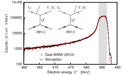
In an inclusive experiment $Q^{2}$ can not be measured directly, which means that looking only at data the initial state radiation processes can not be distinguished from the final state radiation. Hence, in order to get information on $G_{E}^{p}$ at $Q^{2}$ smaller than the elastic setting, the data must be studied in conjunction with a Monte-Carlo simulation, which includes a detailed description of the radiative corrections and considers $G_{E}^{p}$ as its free parameter. This is the basic idea of the MAMI experiment, which opened the door of obtaining $G_{E}^{p}$ down to $Q^{2}\simeq 10^{-4}\,\mathrm{GeV^{2}}/c^{2}$ [9].

The measurement of the radiative tail has been performed at the Mainz Microtron (MAMI) in 2013 using the spectrometer setup of the A1-Collaboration [10]. A rastered electron beam with energies of $E_{0}=195$, $330$ and $495\,\mathrm{MeV}$ was used in combination with a hydrogen target, which consisted of a $5\,\mathrm{cm}$-long cigar-shaped Havar cell filled with liquid hydrogen and placed in an evacuated scattering chamber. For the cross section measurements the single-dipole magnetic spectrometer B was employed at a fixed angle of $15.21^{\circ}$, while its momentum settings were adjusted to scan the complete radiative tail for each beam energy. The central momentum of each setting was measured with an NMR probe to a relative accuracy of $8\times 10^{-5}$. The spectrometer was equipped with the standard detector package consisting of two layers of vertical drift chambers (VDCs) for tracking, two layers of scintillation detectors for triggering, and a threshold Cherenkov detector for particle identification. The kinematic settings of the experiment were chosen such that the radiative tails scanned at three beam energies overlap.

The beam current was between $10\,\mathrm{nA}$ and $1\,\mu\mathrm{A}$ and was limited by the maximum rate allowed in the VDCs ($\approx 1\,\mathrm{kHz/wire}$), resulting in raw rates up to $20\,\mathrm{kHz}$. The beam current was determined by a non-invasive fluxgate-magnetometer and from the collected charge of the beam stopped in a Faraday cup. At low beam currents and low beam energies the accuracy of both approaches is not better than $2\,\mathrm{\%}$, which is insufficient for precise cross section measurements. Hence Spectrometer A was used at a fixed momentum and angular setting for precise monitoring of the relative luminosity.

The analysis of the data, presented in [9], revealed inconsistencies between data and simulation on the order of $10\,\mathrm{\%}$ at the top of the elastic peak, see Fig. 2, which led to the omission of the most statistically relevant, elastic data points in the sample. We believed that the inconsistency arose due to the incomplete theoretical description of the external radiative corrections in the target material in the limit of very small photon energies, which were not considered to the same order of precision as the internal corrections. To be able to incorporate the elastic data in the analysis and ensure a more precise extraction of the proton charge radius, the sensitivity of the results to the applied external radiative corrections and collisional energy losses has been investigated in detail and is shown in Fig. 2.

Figure 2: Relative differences between the data and simulations for the first experimental setup at $495\,\mathrm{MeV}$, including data at the elastic peak and first part of the radiative tail. The blue line shows the original comparison considered in  [9], when the simulation assumes a uniform layer of cryogens around the target cell. The red line corresponds to the result with the artificially amplified external radiative correction given by Mo-Tsai [11]. The green line shows the result achieved with the simulation with enhanced collisional corrections described by the Landau distribution. The black line shows the result with the simulation using an unmodified description of the external corrections but considering that away from the beam, the layer of cryogens is approximately 200 times thicker than along the beam. The red (green) arrow indicates the position of the surplus (deficiency) of events, when using modified radiative (collisional) losses. The systematic uncertainty of all the points is $0.4\,\mathrm{\%}$. The grey band marks the position and width of the elastic line inside the spectrometer acceptance.

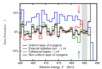
First, the external radiative correction, given by Mo and Tsai [11], were artificially amplified by a factor of $1.44$. This modification brought the simulation into agreement with the data at the elastic peak and below $E^{\prime}=480\,\mathrm{MeV}$, but caused a reduction of simulated events in the first $5\,\mathrm{MeV}$ of the radiative tail. A similar result was observed with the artificial enhancement of collisional corrections described by the Landau distribution, but this time with an excess of simulated events just below the elastic peak. Hence, if both corrections are changed simultaneously, a consistent description of the radiative tail and a correspondingly small relative difference over the whole momentum range are observed. This finding suggests that the observed inconsistency is a consequence of an unaccounted for material traversed by the scattered electrons and is not due to an incomplete description of the applied external corrections. This was confirmed by the dedicated followup experiment, using the same experimental setup but different targets. Data were collected using plastic ($[\mathrm{CH_{2}}]_{n}$) targets with different thicknesses, which created a perfect testbed for validating the applied corrections. The analysis of the elastic peak shapes demonstrated a good agreement between the data and simulations and exhibited the correct scaling of the corrections with the thickness of the target.

In spite of the good vacuum conditions inside the scattering chamber ($10^{-6}\,\mathrm{mbar}$), the experiment was sensitive to traces of cryogenic deposits on the target walls, consisting mostly of residual nitrogen and oxygen present in the scattering chamber [12]. To determine the amount of cryogenic deposits, spectrometer A was positioned such that the nitrogen/oxygen elastic lines were inside its acceptance. The collected spectra, together with the known elastic cross-sections for these elements were used to determine the thickness of the deposited layer. However, the analysis assumed that the layer has the same thickness in all parts of the target cell, disregarding that the depositions on the side walls can be much thicker than those on the end caps, because the former are not heated by the electron beam. Since the material on the side walls is not detectable by the spectrometers, the amount of cryogens was estimated by matching the functional dependence of the simulation to the measured elastic spectra. See Fig. 2. This showed that the layer of cryogens on the side can be as much as $200$ times thicker (roughly $4\cdot 10^{-3}\,\mathrm{g/cm^{2}}$) than at the end caps. This new insight significantly improved the agreement between the data and simulation and allowed us to include the elastic data in a new analysis.

3 Experimental uncertainties

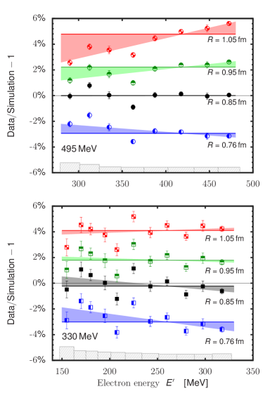
Although the ISR experiment provides remarkable control over the systematic uncertainties, a few ambiguities remain and limit the precision of the results [9]. The contributions relevant for the extraction of the proton charge radius include the uncertainty in the relative luminosity ($0.17\,\mathrm{\%}$), the ambiguity in the detector efficiencies $(0.2\,\mathrm{\%})$ and the contamination coming from the target support frame and the spectrometer entrance flange $(0.4\,\mathrm{\%})$. The portion of the spectrum containing contributions from the pion electroproduction is $0.5\,\mathrm{\%}$, but is significant only for the $495\,\mathrm{MeV}$ setting. The combined point-wise systematic uncertainties are presented in Fig. 3.

4 Extraction of the radius

Following the approach described in [9] the full set of $25$ data points was used to extract the proton-charge form factors for $0.001\leq Q^{2}\leq 0.017\,\mathrm{GeV}^{2}/c^{2}$. The values and the details of the extraction are presented in [13]. These were then compared to the polynomial function

$$G(Q^{2})=n_{E_{0}}\left[1-\frac{r_{p}^{2}\,Q^{2}}{6\,\hbar^{2}}+\frac{a\,Q^{4}}{120\,\hbar^{4}}-\frac{b\,Q^{6}}{5040\,\hbar^{6}}\right]\,,$$ (2)

where parameters $a=(2.59\pm 0.194)\,\mathrm{fm}^{4}$ and $b=(29.8\pm 14.71)\,\mathrm{fm}^{6}$, which determine the curvature of the fit, were taken from Ref. [14]. The three data sets were fit with a common parameter for the radius, $r_{p}$, but with different renormalisation factors, $n_{E_{0}}$, for each energy. In terms of this fit with $21$ degrees of freedom and $\chi^{2}$ of $95.4$, the normalisations and the radius were determined to be:

$$n_{195} = 1.002\pm 0.002_{\mathrm{stat}}\pm 0.007_{\mathrm{syst}}\,,$$

$$n_{330} = 1.000\pm 0.001_{\mathrm{stat}}\pm 0.003_{\mathrm{syst}}\,,$$

$$n_{495} = 0.999\pm 0.001_{\mathrm{stat}}\pm 0.004_{\mathrm{syst}}\,,$$

$$r_{p} = (0.836\pm 0.017_{\mathrm{stat}}\pm 0.059_{\mathrm{syst}}\pm 0.003_{mod})\,\mathrm{fm}\,.$$

The value of $\chi^{2}$ has almost doubled with respect to the previous dataset [9], but this is due to the addition of three statistically very precise points at $Q^{2}=0.017\,\mathrm{GeV^{2}}/c^{2}$, $0.008\,\mathrm{GeV^{2}}/c^{2}$ and $0.003\,\mathrm{GeV^{2}}/c^{2}$. On the other hand, even by including these points and improving the analysis in the above manner, the extracted radius remains governed by the systematic uncertainty and still critically depends on the available $Q^{2}$ range and the number of fitting parameters.

To improve these results within the scope of available data, an alternative approach was considered, applicable at the level of measured cross-sections. To first order the $E^{\prime}$ evolution of the ratio between the data and the simulation, $R_{i}(r_{p})$, at each energy setting depends only on the proton charge radius. Here, index $i$ denotes the kinematic setting with energy $E^{\prime}$. Furthermore, since all points for a single energy configuration are strongly correlated due to the nature of the experimental approach the effect of changing the radius appears as a change of the slope of the ratio. Hence, focusing on the slopes of the cross-section ratios effectively eliminates normalisations from the minimisation procedure and offers more accurate determination of the radius. To evaluate the sensitivity of the data to the proton charge radius, the simulation with the same form-factor model (2) was run for 10 different values of $r_{p}$ between $0.76\,\mathrm{fm}$ and $1.05\,\mathrm{fm}$. The results of the comparison have demonstrated that only at the highest two energy settings ($330\,\mathrm{MeV}$ and $495\,\mathrm{MeV}$) the $Q^{2}$ is large enough for the measurements to be sensitive to small changes in the proton radius. See Fig. 3. The data at $195\,\mathrm{MeV}$ exhibit no detectable dependence on the proton charge radius and, within the measured uncertainties, could be used only for the absolute calibration of the measured cross-sections.

Relying on the chosen model (2), the best estimate for the proton charge radius should return a flat ratio between the data and the simulation as a function of $E^{\prime}$. The ratios obtained with different values of the parameter, presented in Fig. 3, demonstrate that the $495\,\mathrm{MeV}$ setting favours a radius of $\approx 0.85\,\mathrm{fm}$, while the $330\,\mathrm{MeV}$ data suggest $\approx 0.95\,\mathrm{fm}$. To quantify the level of agreement between the data and the simulation performed with a particular value of $r_{p}$, the following function was considered:

$$S(r_{p})=\sum_{i=1}^{N_{495}}\frac{\left(R_{i}(r_{p})-\overline{R}_{495}(r_{p})\right)^{2}}{{\sigma_{R}}_{i}^{2}}+\sum_{j=1}^{N_{330}}\frac{\left(R_{j}(r_{p})-\overline{R}_{330}(r_{p})\right)^{2}}{{\sigma_{R}}_{j}^{2}}\,.$$

For a given value of $r_{p}$ the $\overline{R}_{330}(r_{p})$ and $\overline{R}_{495}(r_{p})$ represent weighted averages of ratios $R_{i}$ and $R_{j}$, while $N_{330}$ and $N_{495}$ correspond to the number of measured points for $330\,\mathrm{MeV}$ and $495\,\mathrm{MeV}$ configuration, respectively. The ${\sigma_{R}}_{i(j)}$ represent the total uncertainties of the measured ratios. The values of $S(r_{p})$ obtained for the selected radii are shown in Fig. 4. Finding a radius that best matches both data sets amounts to finding the minimum of the function $S(r_{p})$ . Unfortunately, the full numerical minimisation of the function could not be performed, because it would require numerous repetitions of the full simulation, which is computationally very intensive. Instead, the simulated points were fitted by a parabola and the radius was determined by finding its vertex at $r_{p}=0.870\,\mathrm{fm}$ and $S=14.89$.

Figure 3: Relative differences between the data and simulations $R_{i(j)}(r_{p})$ for $495\,\mathrm{MeV}$ (top) and $330\,\mathrm{MeV}$ (bottom) settings. Each set of ratios corresponds to simulations with a different value of the proton charge radius $r_{p}=0.76\,\mathrm{fm}$ (blue), $0.85\,\mathrm{fm}$ (black), $0.95\,\mathrm{fm}$ (green) and $1.05\,\mathrm{fm}$ (red). The weighted averages $\overline{R}_{330}(r_{p})$ and $\overline{R}_{495}(r_{p})$ are shown with full lines and are offset from zero for clarity. The sizes of the corresponding triangular shapes denote the magnitude of the inconsistency between the data and simulation. Gray boxes demonstrate the systematic uncertainties.

Figure 4: Top: The blue circles show $S(r_{p})$ corresponding to the comparison of the data to the simulations ran with $r_{p}=0.76$, $0.78$, $0.80$, $0.84$, $0.85$, $0.88$, $0.90$, $0.95$, $0.99$, and $1.05\,\mathrm{fm}$. The red curve represents the parabola fitted to the blue points. The horizontal line marks the number of degrees of freedom and should ideally agree with the minimal value of the fit function. The green curves represent parabolas, when data points are randomly smeared by their uncertainties. Bottom: The histogram shows the distribution of minima of the parabolas shown in the upper panel. The extracted radius presented with the black point corresponds to the minimum of the red parabola in the upper panel. Its uncertainty is determined by the width of the distribution of minima.

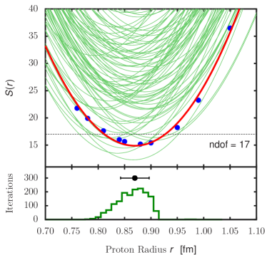
Furthermore, $S(r_{p})$ can be recognized as a $\chi^{2}$ estimator of the quality of the fit. One expects $N_{330}+N_{495}-2=17$ number of degrees of freedom, indicating that the fit reliably describes the data.

The uncertainty of the extracted radius was determined by means of a Monte-Carlo simulation. In each iteration the extracted ratios $R_{i(j)}$ were changed randomly following a Gaussian distribution with a width given by ${\sigma_{R}}_{i(j)}$. Additionally, since only one set of data is available and only the simulation is changing in the study, the points at the same energy (or index $i,j$) simulated with different radii are correlated. Hence, they need to be offset simultaneously by the same amount. The applied changes result in a different minimisation parabola and different radius. Repeating the simulation many times, considering both statistical and systematic uncertainties, results in a distribution of radii, see Fig. 4 (bottom), whose width serves as an estimation of the uncertainty of the extracted proton charge radius. The best value for the proton charge radius becomes:

$$r_{p}=\left(0.870\pm 0.014_{\mathrm{stat.}}\pm 0.024_{\mathrm{sys.}}\pm 0.003_{\mathrm{mod.}}\right)\,\mathrm{fm}\,.$$

The presented result contains a small model dependence on the function (2) used to describe $G_{E}^{p}$. The model uncertainty arises from the uncertainties of the parameters $a$ and $b$, which are robust and based on the data of Bernauer et al. [15]. While our data are not precise enough for independent extraction of $a$ and $b$, the radius extraction procedure is sensitive to their specific value. Replacing $a$ and $b$ by those obtained from the ChPT calculations of Alarcon and Weiss [16], for instance would increase the function $S$, while the resulting radius would shift by about $-0.015\,\mathrm{fm}$ towards a smaller value.

5 Conclusions

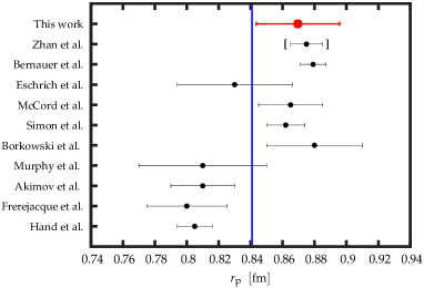
The initial state radiation experiment at MAMI [9] established a new method for precise investigations of the electromagnetic structure of the nucleon and underlying electromagnetic processes at extremely small $Q^{2}$. In this paper we present our findings on the improved data analysis, which revealed the necessity of a complete consideration of cryogens deposited on the liquid hydrogen cell and their influence on the $e$-$p$ scattering results. The analysis also demonstrated the precision with which these effects could be studied and offered new, improved values of the $G_{E}^{p}$ not accessible in the original work. Furthermore, by studying the slopes of the measured radiative tails relative to the simulated ones, an alternative approach for the extraction of the proton charge radius was developed, which yielded a competitive new value (see Fig. 5) and improved the precision of our initial result [9] by almost a factor of $3$.

Figure 5: The proton charge radius extracted from the ISR experiment together with previous electron scattering measurements [17, 18, 19, 20, 21, 22, 23, 24, 25], where the data point of Zhan et al., enclosed by square brackets, is not an independent measurement of the radius [26]. The value obtained from the Lamb shift measurements in muonic hydrogen is shown by the blue line for the comparison.

References

- [1] P. J. Mohr, D. B. Newell, B. N. Taylor, Codata recommended values of the fundamental physical constants: 2014, Rev. Mod. Phys. 88 (2016) 035009. doi:10.1103/RevModPhys.88.035009.
- [2] R. Pohl, et al., The size of the proton, Nature 466 (2010) 213–216.
- [3] A. Antognini, et al., Proton structure from the measurement of 2s-2p transition frequencies of muonic hydrogen, Science 339 (2013) 417–420. doi:10.1126/science.1230016.
-
[4]
A. Beyer, L. Maisenbacher, A. Matveev, R. Pohl, K. Khabarova, A. Grinin,
T. Lamour, D. C. Yost, T. W. Hänsch, N. Kolachevsky, T. Udem,
The rydberg constant
and proton size from atomic hydrogen, Science 358 (2017) 79–85.
arXiv:http://science.sciencemag.org/content/358/6359/79.full.pdf,
doi:10.1126/science.aah6677.
URL http://science.sciencemag.org/content/358/6359/79 -
[5]
H. Fleurbaey, S. Galtier, S. Thomas, M. Bonnaud, L. Julien, F. m. c. Biraben,
F. m. c. Nez, M. Abgrall, J. Guéna,
New
measurement of the transition frequency of hydrogen:
Contribution to the proton charge radius puzzle, Phys. Rev. Lett. 120 (2018)
183001.
doi:10.1103/PhysRevLett.120.183001.
URL https://link.aps.org/doi/10.1103/PhysRevLett.120.183001 - [6] R. Pohl, R. Gilman, G. A. Miller, K. Pachucki, Muonic hydrogen and the proton radius puzzle, Ann. Rev. Nucl. Part. Sci. 63 (2013) 175–204. doi:10.1146/annurev-nucl-102212-170627.
- [7] C. E. Carlson, The proton radius puzzle, Prog. Part. Nucl. Phys. 82 (2015) 59–77. doi:http://dx.doi.org/10.1016/j.ppnp.2015.01.002.
- [8] M. Vanderhaeghen, J. M. Friedrich, D. Lhuillier, D. Marchand, L. Van Hoorebeke, J. Van de Wiele, Qed radiative corrections to virtual compton scattering, Phys. Rev. C 62 (2000) 025501. doi:10.1103/PhysRevC.62.025501.
- [9] M. Mihovilovič, et al., First measurement of proton’s charge form factor at very low with initial state radiation, Phys. Lett. B 771 (2017) 194–198. arXiv:1612.06707, doi:10.1016/j.physletb.2017.05.031.
- [10] K. Blomqvist, et al., The three-spectrometer facility at the mainz microtron {MAMI}, Nucl. Instr. and Meth. A 403 (1998) 263–301. doi:http://dx.doi.org/10.1016/S0168-9002(97)01133-9.
- [11] L. W. Mo, Y. S. Tsai, Radiative corrections to elastic and inelastic and scattering, Rev. Mod. Phys. 41 (1969) 205–235. doi:10.1103/RevModPhys.41.205.
- [12] M. Mihovilovič, et al., Initial state radiation experiment at MAMI, EPJ Web Conf. 72 (2014) 00017. doi:10.1051/epjconf/20147200017.
- [13] M. Mihovilovic, et al., See supplemental material for more details.
- [14] M. O. Distler, J. C. Bernauer, T. Walcher, The {RMS} charge radius of the proton and zemach moments, Phys. Lett. B 696 (2011) 343–347. doi:http://dx.doi.org/10.1016/j.physletb.2010.12.067.
[15]
J. C. Bernauer, M. O. Distler, J. Friedrich, T. Walcher, P. Achenbach,
C. Ayerbe Gayoso, R. Böhm, D. Bosnar, L. Debenjak, L. Doria, A. Esser,
H. Fonvieille, M. Gómez Rodríguez de la Paz, J. M. Friedrich,
M. Makek, H. Merkel, D. G. Middleton, U. Müller, L. Nungesser,
J. Pochodzalla, M. Potokar, S. Sánchez Majos, B. S. Schlimme,
S. Širca, M. Weinriefer,
Electric and
magnetic form factors of the proton, Phys. Rev. C 90 (2014) 015206.
doi:10.1103/PhysRevC.90.015206.
URL https://link.aps.org/doi/10.1103/PhysRevC.90.015206 -
[16]
J. M. Alarcón, C. Weiss,
Nucleon form
factors in dispersively improved chiral effective field theory. ii.
electromagnetic form factors, Phys. Rev. C 97 (2018) 055203.
doi:10.1103/PhysRevC.97.055203.
URL https://link.aps.org/doi/10.1103/PhysRevC.97.055203 -
[17]
L. N. Hand, D. G. Miller, R. Wilson,
magnetic form factors of the nucleon, Rev. Mod. Phys. 35 (1963) 335–349.
doi:10.1103/RevModPhys.35.335.
URL https://link.aps.org/doi/10.1103/RevModPhys.35.335 -
[18]
D. Frèrejacque, D. Benaksas, D. Drickey,
Proton form factors
from observation of recoil protons, Phys. Rev. 141 (1966) 1308–1312.
doi:10.1103/PhysRev.141.1308.
URL https://link.aps.org/doi/10.1103/PhysRev.141.1308 - [19] Yu. K. Akimov, et al., Small angle scattering of electrons by protons, Sov. Phys. JETP 35 (1972) 651–654, [Zh. Eksp. Teor. Fiz. 62, 1231 (1972)].
[20]
J. J. Murphy, Y. M. Shin, D. M. Skopik,
Proton form factor
from 0.15 to 0.79 , Phys. Rev. C 9 (1974)
2125–2129.
doi:10.1103/PhysRevC.9.2125.
URL https://link.aps.org/doi/10.1103/PhysRevC.9.2125 - [21] F. Borkowski, G. G. Simon, V. H. Walther, R. D. Wendling, On the determination of the proton RMS-radius from electron scattering data, Z. Phys. A275 (1975) 29–31. doi:10.1007/BF01409496.
- [22] G. Simon, C. Schmitt, F. Borkowski, V. Walther, Absolute electron-proton cross sections at low momentum transfer measured with a high pressure gas target system, Nucl. Phys. A 333 (1980) 381–391. doi:http://dx.doi.org/10.1016/0375-9474(80)90104-9.
- [23] M. McCord, H. Crannell, L. W. Fagg, J. T. O’Brien, D. I. Sober, J. W. Lightbody, X. K. Maruyama, P. A. Treado, Preliminary results of a new determination of the rms charge radius of the proton, Nucl. Instrum. Meth. B 56-57 (1991) 496–499. doi:10.1016/0168-583X(91)96079-Z.
[24]
I. Eschrich, et al., Physics Letters B 522 (2001) 233–239.
doi:https://doi.org/10.1016/S0370-2693(01)01285-0,
[link].
URL http://www.sciencedirect.com/science/article/pii/S0370269301012850 - [25] J. C. Bernauer, et al., High-precision determination of the electric and magnetic form factors of the proton, Phys. Rev. Lett. 105 (2010) 242001. doi:10.1103/PhysRevLett.105.242001.
- [26] X. Zhan, et al., High-precision measurement of the proton elastic form factor ratio at low, Physics Letters B 705 (2011) 59–64. doi:http://dx.doi.org/10.1016/j.physletb.2011.10.002.