Four electron spin qubits with exchange interaction

H.W.L. Naus Quantum Technology, TNO, P.O. Box 155, 2600 AD Delft and QuTech, Delft University of Technology, P.O. Box 5046, 2600 GA Delft, The Netherlands
Abstract

Four electron spin qubits in quantum dots are studied by means of an exchange interaction Hamiltonian. The time-independent SchrΓΆdinger equation is exactly analytically solved for the symmetric case, that is equal qubit frequencies and equal couplings. The spin system can be used as two data-qubits and two ancillas, thereby realizing a X𝑋X and Z𝑍Z stabilizing circuit exploited in error correction and surface codes. The unitary evolution of corresponding stable states is calculated and consequences for error syndromes and fidelities are assessed. It is also shown that applying the evolution operator for a prescribed duration and subsequent measurement of the ancillas lead to a β€˜verifiable’ two-qubit phase gate.

I Introduction

In this study, we consider four electron spin qubits in quantum dots, which interact via an exchange Hamiltonian. Such a few-qubit system can serve as a simple stabilizing circuit exploited in error correction for fault-tolerant quantum computing. It also may be used as unit cell in a scalable many spin qubit quantum processor.

The reviews Engel ; Hanson , the thesis Kawa and references therein introduce the basics of electron spins in quantum dots. The essential ingredient is the description of the low-energy physics of electrons in quantum dots by the exchange Hamiltonian, as argued in the seminal papers Loss98 ; Loss00 . The Heisenberg interaction for two confined electrons takes their Coulomb interaction and the Pauli exclusion principle effectively into account Ash . For electrons in quantum dots the possible tunneling process is included in Meun ; Watson by enlarging the 4D two-spin Hilbert space to a 6D space. In Meun the effective exchange interaction is rederived. Note that turning the tunneling on and off results in a time-dependent exchange coupling Loss98 ; Loss00 . Here we restrict ourselves to constant coupling; if it is taken to be equal for the interacting pairs of spin, the problem can be analytically exactly solved in the resonant case. Slightly different qubit frequencies may be taken into account perturbatively; we also present the explicit form of this perturbation.

After solving the model Hamiltonian, we address the unitary evolution of the stable states used in the X𝑋X and Z𝑍Z stabilizer circuits as introduced in Fowler . Two qubits are considered as data qubits, whereas the other two are ancillas which are supposed to be measured. It is completely analogous to the recent analysis Naus-stab of a coupled qubit-resonator system. Of course, the degrees of freedom and their dynamics are different. Therefore, we refer to Naus-stab for further discussion and motivation of the followed approach. Our calculations have also demonstrated the possible implementation of phase gates for the data-qubits. They may be called β€˜checkable’ or β€˜verifiable’ gates because of concomitant ancilla measurements.

The outline of this paper is as follows. First, the exchange Hamiltonian of four interacting spins in a magnetic field is presented and solved for equal couplings and frequencies. In section III, the general final state of the stabilizing circuit is rewritten in terms of singlet-triplet states. Subsequent unitary evolution and consequences for probabilities and fidelities are calculated in section IV. The next section V demonstrates the concept of verifiable gates. The final section presents conclusions.

II Four interacting spins

In order to analyze a simple stabilizer Fowler , we consider a spin system consisting out of two data qubits Q1,Q2subscript𝑄1subscript𝑄2Q_{1},Q_{2} and and two ancillas Qa,Qbsubscriptπ‘„π‘Žsubscript𝑄𝑏Q_{a},Q_{b}. They are arranged as shown in the figure and only nearest neighbour interaction, indicated by the dashed red lines, is included.

Q1subscript𝑄1Q_{1}Qasubscriptπ‘„π‘ŽQ_{a}Qbsubscript𝑄𝑏Q_{b}Q2subscript𝑄2Q_{2}

The model Hamiltonian incorporating the exchange interaction is taken as

H𝐻\displaystyle H =\displaystyle= H0+Hintsubscript𝐻0subscript𝐻int\displaystyle H_{0}+H_{\text{int}} (1)
=\displaystyle= ω​(Sz[1]+Sz[2])+Ο‰~​(Sz[a]+Sz[b])πœ”superscriptsubscript𝑆𝑧delimited-[]1superscriptsubscript𝑆𝑧delimited-[]2~πœ”superscriptsubscript𝑆𝑧delimited-[]π‘Žsuperscriptsubscript𝑆𝑧delimited-[]𝑏\displaystyle\omega(S_{z}^{[1]}+S_{z}^{[2]})+\tilde{\omega}(S_{z}^{[a]}+S_{z}^{[b]})
+\displaystyle+ π’₯​(Sβ†’[1]β‹…Sβ†’[a]+Sβ†’[1]β‹…Sβ†’[b]+Sβ†’[2]β‹…Sβ†’[a]+Sβ†’[2]β‹…Sβ†’[b])π’₯β‹…superscript→𝑆delimited-[]1superscript→𝑆delimited-[]π‘Žβ‹…superscript→𝑆delimited-[]1superscript→𝑆delimited-[]𝑏⋅superscript→𝑆delimited-[]2superscript→𝑆delimited-[]π‘Žβ‹…superscript→𝑆delimited-[]2superscript→𝑆delimited-[]𝑏\displaystyle\mathcal{J}(\vec{S}^{[1]}\cdot\vec{S}^{[a]}+\vec{S}^{[1]}\cdot\vec{S}^{[b]}+\vec{S}^{[2]}\cdot\vec{S}^{[a]}+\vec{S}^{[2]}\cdot\vec{S}^{[b]})
=\displaystyle= ω​(Sz[1]+Sz[2])+Ο‰~​(Sz[a]+Sz[b])πœ”superscriptsubscript𝑆𝑧delimited-[]1superscriptsubscript𝑆𝑧delimited-[]2~πœ”superscriptsubscript𝑆𝑧delimited-[]π‘Žsuperscriptsubscript𝑆𝑧delimited-[]𝑏\displaystyle\omega(S_{z}^{[1]}+S_{z}^{[2]})+\tilde{\omega}(S_{z}^{[a]}+S_{z}^{[b]})
+\displaystyle+ π’₯​(Sβ†’[1]+Sβ†’[2])β‹…(Sβ†’[a]+Sβ†’[b]).β‹…π’₯superscript→𝑆delimited-[]1superscript→𝑆delimited-[]2superscript→𝑆delimited-[]π‘Žsuperscript→𝑆delimited-[]𝑏\displaystyle\mathcal{J}(\vec{S}^{[1]}+\vec{S}^{[2]})\cdot(\vec{S}^{[a]}+\vec{S}^{[b]}).

The β€˜free’ Hamiltonian represents the energy of the electron spins in a homogeneous magnetic field in the z𝑧z-direction. The electron spin operators are related to the Pauli matrices

Sk=12​ℏ​σk,k=x,y,z.formulae-sequencesubscriptπ‘†π‘˜12Planck-constant-over-2-pisubscriptπœŽπ‘˜π‘˜π‘₯𝑦𝑧S_{k}=\tfrac{1}{2}\hbar\sigma_{k},\quad k=x,y,z. (2)

The constant π’₯π’₯\mathcal{J} is is commonly known as the exchange interaction strength. After introducing the total four-spin operator J→→𝐽\vec{J} as

Jβ†’=Sβ†’[1]+Sβ†’[2]+Sβ†’[a]+Sβ†’[b],→𝐽superscript→𝑆delimited-[]1superscript→𝑆delimited-[]2superscript→𝑆delimited-[]π‘Žsuperscript→𝑆delimited-[]𝑏\vec{J}=\vec{S}^{[1]}+\vec{S}^{[2]}+\vec{S}^{[a]}+\vec{S}^{[b]}, (3)

the interaction Hamiltonian can be rewritten as

Hint=12​π’₯​(Jβ†’2βˆ’(Sβ†’[1]+Sβ†’[2])2βˆ’(Sβ†’[a]+Sβ†’[b])2).subscript𝐻int12π’₯superscript→𝐽2superscriptsuperscript→𝑆delimited-[]1superscript→𝑆delimited-[]22superscriptsuperscript→𝑆delimited-[]π‘Žsuperscript→𝑆delimited-[]𝑏2H_{\text{int}}=\tfrac{1}{2}\mathcal{J}\left(\vec{J}^{2}-\left(\vec{S}^{[1]}+\vec{S}^{[2]}\right)^{2}-\left(\vec{S}^{[a]}+\vec{S}^{[b]}\right)^{2}\right). (4)

It suggests the following construction of basis states. First, the data qubits are combined as singlet and triplet states; the same is done for the ancillas. Thus we have defined the respective two-qubit bases

|S[12]⟩,|T+[12]⟩,|T0[12]⟩,|Tβˆ’[12]⟩andketsuperscript𝑆delimited-[]12ketsuperscriptsubscript𝑇delimited-[]12ketsuperscriptsubscript𝑇0delimited-[]12ketsuperscriptsubscript𝑇delimited-[]12and\displaystyle|S^{[12]}\rangle,|T_{+}^{[12]}\rangle,|T_{0}^{[12]}\rangle,|T_{-}^{[12]}\rangle\quad\text{and}
|S[a​b]⟩,|T+[a​b]⟩,|T0[a​b]⟩,|Tβˆ’[a​b]⟩.ketsuperscript𝑆delimited-[]π‘Žπ‘ketsuperscriptsubscript𝑇delimited-[]π‘Žπ‘ketsuperscriptsubscript𝑇0delimited-[]π‘Žπ‘ketsuperscriptsubscript𝑇delimited-[]π‘Žπ‘\displaystyle|S^{[ab]}\rangle,|T_{+}^{[ab]}\rangle,|T_{0}^{[ab]}\rangle,|T_{-}^{[ab]}\rangle. (5)

Four-qubit basis states are now constructed by combining the two singlets, one singlet with a triplet yielding spin 1 β€˜particles’ and the two triplets yielding a spin 0, a spin 1 and a spin 2 β€˜particle’. We explicitly obtain for the singlets

|e1⟩=|S[12]βŸ©βŠ—|S[a​b]⟩(j,mj)=(0,0)formulae-sequenceketsubscript𝑒1tensor-productketsuperscript𝑆delimited-[]12ketsuperscript𝑆delimited-[]π‘Žπ‘π‘—subscriptπ‘šπ‘—00|e_{1}\rangle=|S^{[12]}\rangle\otimes|S^{[ab]}\rangle\qquad(j,m_{j})=(0,0) (6)

and for the singlet triplet combinations

|e2⟩ketsubscript𝑒2\displaystyle|e_{2}\rangle =\displaystyle= |S[12]βŸ©βŠ—|T+[a​b]⟩(j,mj)=(1,1),tensor-productketsuperscript𝑆delimited-[]12ketsuperscriptsubscript𝑇delimited-[]π‘Žπ‘π‘—subscriptπ‘šπ‘—11\displaystyle|S^{[12]}\rangle\otimes|T_{+}^{[ab]}\rangle\qquad(j,m_{j})=(1,1),
|e3⟩ketsubscript𝑒3\displaystyle|e_{3}\rangle =\displaystyle= |S[12]βŸ©βŠ—|T0[a​b]⟩(j,mj)=(1,0),tensor-productketsuperscript𝑆delimited-[]12ketsuperscriptsubscript𝑇0delimited-[]π‘Žπ‘π‘—subscriptπ‘šπ‘—10\displaystyle|S^{[12]}\rangle\otimes|T_{0}^{[ab]}\rangle\qquad(j,m_{j})=(1,0),
|e4⟩ketsubscript𝑒4\displaystyle|e_{4}\rangle =\displaystyle= |S[12]βŸ©βŠ—|Tβˆ’[a​b]⟩(j,mj)=(1,βˆ’1),tensor-productketsuperscript𝑆delimited-[]12ketsuperscriptsubscript𝑇delimited-[]π‘Žπ‘π‘—subscriptπ‘šπ‘—11\displaystyle|S^{[12]}\rangle\otimes|T_{-}^{[ab]}\rangle\qquad(j,m_{j})=(1,-1),
|e5⟩ketsubscript𝑒5\displaystyle|e_{5}\rangle =\displaystyle= |T+[12]βŸ©βŠ—|S[a​b]⟩(j,mj)=(1,1),tensor-productketsuperscriptsubscript𝑇delimited-[]12ketsuperscript𝑆delimited-[]π‘Žπ‘π‘—subscriptπ‘šπ‘—11\displaystyle|T_{+}^{[12]}\rangle\otimes|S^{[ab]}\rangle\qquad(j,m_{j})=(1,1),
|e6⟩ketsubscript𝑒6\displaystyle|e_{6}\rangle =\displaystyle= |T0[12]βŸ©βŠ—|S[a​b]⟩(j,mj)=(1,0),tensor-productketsuperscriptsubscript𝑇0delimited-[]12ketsuperscript𝑆delimited-[]π‘Žπ‘π‘—subscriptπ‘šπ‘—10\displaystyle|T_{0}^{[12]}\rangle\otimes|S^{[ab]}\rangle\qquad(j,m_{j})=(1,0),
|e7⟩ketsubscript𝑒7\displaystyle|e_{7}\rangle =\displaystyle= |Tβˆ’[12]βŸ©βŠ—|S[a​b]⟩(j,mj)=(1,βˆ’1).tensor-productketsuperscriptsubscript𝑇delimited-[]12ketsuperscript𝑆delimited-[]π‘Žπ‘π‘—subscriptπ‘šπ‘—11\displaystyle|T_{-}^{[12]}\rangle\otimes|S^{[ab]}\rangle\qquad(j,m_{j})=(1,-1). (7)

We have indicated the quantum numbers of the total spin of the states. Combining the triplets yields Cohen2 the scalar

|e8⟩=13​3​{|T+[12]βŸ©βŠ—|Tβˆ’[a​b]βŸ©βˆ’|T0[12]βŸ©βŠ—|T0[a​b]⟩+|Tβˆ’[12]βŸ©βŠ—|T+[a​b]⟩}(j,mj)=(0,0)formulae-sequenceketsubscript𝑒8133tensor-productketsuperscriptsubscript𝑇delimited-[]12ketsuperscriptsubscript𝑇delimited-[]π‘Žπ‘tensor-productketsuperscriptsubscript𝑇0delimited-[]12ketsuperscriptsubscript𝑇0delimited-[]π‘Žπ‘tensor-productketsuperscriptsubscript𝑇delimited-[]12ketsuperscriptsubscript𝑇delimited-[]π‘Žπ‘π‘—subscriptπ‘šπ‘—00|e_{8}\rangle=\tfrac{1}{3}\sqrt{3}\left\{|T_{+}^{[12]}\rangle\otimes|T_{-}^{[ab]}\rangle-|T_{0}^{[12]}\rangle\otimes|T_{0}^{[ab]}\rangle+|T_{-}^{[12]}\rangle\otimes|T_{+}^{[ab]}\rangle\right\}\qquad(j,m_{j})=(0,0) (8)

and the spin 1 states

|e9⟩ketsubscript𝑒9\displaystyle|e_{9}\rangle =\displaystyle= 12​2​{|T+[12]βŸ©βŠ—|T0[a​b]βŸ©βˆ’|T0[12]βŸ©βŠ—|T+[a​b]⟩}(j,mj)=(1,1),122tensor-productketsuperscriptsubscript𝑇delimited-[]12ketsuperscriptsubscript𝑇0delimited-[]π‘Žπ‘tensor-productketsuperscriptsubscript𝑇0delimited-[]12ketsuperscriptsubscript𝑇delimited-[]π‘Žπ‘π‘—subscriptπ‘šπ‘—11\displaystyle\tfrac{1}{2}\sqrt{2}\left\{|T_{+}^{[12]}\rangle\otimes|T_{0}^{[ab]}\rangle-|T_{0}^{[12]}\rangle\otimes|T_{+}^{[ab]}\rangle\right\}\quad(j,m_{j})=(1,1),
|e10⟩ketsubscript𝑒10\displaystyle|e_{10}\rangle =\displaystyle= 12​2​{|T+[12]βŸ©βŠ—|Tβˆ’[a​b]βŸ©βˆ’|Tβˆ’[12]βŸ©βŠ—|T+[a​b]⟩}(j,mj)=(1,0),122tensor-productketsuperscriptsubscript𝑇delimited-[]12ketsuperscriptsubscript𝑇delimited-[]π‘Žπ‘tensor-productketsuperscriptsubscript𝑇delimited-[]12ketsuperscriptsubscript𝑇delimited-[]π‘Žπ‘π‘—subscriptπ‘šπ‘—10\displaystyle\tfrac{1}{2}\sqrt{2}\left\{|T_{+}^{[12]}\rangle\otimes|T_{-}^{[ab]}\rangle-|T_{-}^{[12]}\rangle\otimes|T_{+}^{[ab]}\rangle\right\}\quad(j,m_{j})=(1,0),
|e11⟩ketsubscript𝑒11\displaystyle|e_{11}\rangle =\displaystyle= 12​2​{|T0[12]βŸ©βŠ—|Tβˆ’[a​b]βŸ©βˆ’|Tβˆ’[12]βŸ©βŠ—|T0[a​b]⟩}(j,mj)=(1,βˆ’1).122tensor-productketsuperscriptsubscript𝑇0delimited-[]12ketsuperscriptsubscript𝑇delimited-[]π‘Žπ‘tensor-productketsuperscriptsubscript𝑇delimited-[]12ketsuperscriptsubscript𝑇0delimited-[]π‘Žπ‘π‘—subscriptπ‘šπ‘—11\displaystyle\tfrac{1}{2}\sqrt{2}\left\{|T_{0}^{[12]}\rangle\otimes|T_{-}^{[ab]}\rangle-|T_{-}^{[12]}\rangle\otimes|T_{0}^{[ab]}\rangle\right\}\quad(j,m_{j})=(1,-1). (9)

Finally, we get the resulting spin 2 states

|e12⟩ketsubscript𝑒12\displaystyle|e_{12}\rangle =\displaystyle= |T+[12]βŸ©βŠ—|T+[a​b]⟩(j,mj)=(2,2),tensor-productketsuperscriptsubscript𝑇delimited-[]12ketsuperscriptsubscript𝑇delimited-[]π‘Žπ‘π‘—subscriptπ‘šπ‘—22\displaystyle|T_{+}^{[12]}\rangle\otimes|T_{+}^{[ab]}\rangle\qquad(j,m_{j})=(2,2),
|e13⟩ketsubscript𝑒13\displaystyle|e_{13}\rangle =\displaystyle= 12​2​{|T+[12]βŸ©βŠ—|T0[a​b]⟩+|T0[12]βŸ©βŠ—|T+[a​b]⟩}(j,mj)=(2,1),122tensor-productketsuperscriptsubscript𝑇delimited-[]12ketsuperscriptsubscript𝑇0delimited-[]π‘Žπ‘tensor-productketsuperscriptsubscript𝑇0delimited-[]12ketsuperscriptsubscript𝑇delimited-[]π‘Žπ‘π‘—subscriptπ‘šπ‘—21\displaystyle\tfrac{1}{2}\sqrt{2}\left\{|T_{+}^{[12]}\rangle\otimes|T_{0}^{[ab]}\rangle+|T_{0}^{[12]}\rangle\otimes|T_{+}^{[ab]}\rangle\right\}\qquad(j,m_{j})=(2,1),
|e14⟩ketsubscript𝑒14\displaystyle|e_{14}\rangle =\displaystyle= 16​6​{|T+[12]βŸ©βŠ—|Tβˆ’[a​b]⟩+2​|T0[12]βŸ©βŠ—|T0[a​b]⟩+|Tβˆ’[12]βŸ©βŠ—|T+[a​b]⟩}(j,mj)=(2,0),166tensor-productketsuperscriptsubscript𝑇delimited-[]12ketsuperscriptsubscript𝑇delimited-[]π‘Žπ‘tensor-product2ketsuperscriptsubscript𝑇0delimited-[]12ketsuperscriptsubscript𝑇0delimited-[]π‘Žπ‘tensor-productketsuperscriptsubscript𝑇delimited-[]12ketsuperscriptsubscript𝑇delimited-[]π‘Žπ‘π‘—subscriptπ‘šπ‘—20\displaystyle\tfrac{1}{6}\sqrt{6}\left\{|T_{+}^{[12]}\rangle\otimes|T_{-}^{[ab]}\rangle+2|T_{0}^{[12]}\rangle\otimes|T_{0}^{[ab]}\rangle+|T_{-}^{[12]}\rangle\otimes|T_{+}^{[ab]}\rangle\right\}\quad(j,m_{j})=(2,0),
|e15⟩ketsubscript𝑒15\displaystyle|e_{15}\rangle =\displaystyle= 12​2​{|T0[12]βŸ©βŠ—|Tβˆ’[a​b]⟩+|Tβˆ’[12]βŸ©βŠ—|T0[a​b]⟩}(j,mj)=(2,βˆ’1),122tensor-productketsuperscriptsubscript𝑇0delimited-[]12ketsuperscriptsubscript𝑇delimited-[]π‘Žπ‘tensor-productketsuperscriptsubscript𝑇delimited-[]12ketsuperscriptsubscript𝑇0delimited-[]π‘Žπ‘π‘—subscriptπ‘šπ‘—21\displaystyle\tfrac{1}{2}\sqrt{2}\left\{|T_{0}^{[12]}\rangle\otimes|T_{-}^{[ab]}\rangle+|T_{-}^{[12]}\rangle\otimes|T_{0}^{[ab]}\rangle\right\}\qquad(j,m_{j})=(2,-1),
|e16⟩ketsubscript𝑒16\displaystyle|e_{16}\rangle =\displaystyle= |Tβˆ’[12]βŸ©βŠ—|Tβˆ’[a​b]⟩(j,mj)=(2,βˆ’2).tensor-productketsuperscriptsubscript𝑇delimited-[]12ketsuperscriptsubscript𝑇delimited-[]π‘Žπ‘π‘—subscriptπ‘šπ‘—22\displaystyle|T_{-}^{[12]}\rangle\otimes|T_{-}^{[ab]}\rangle\qquad(j,m_{j})=(2,-2). (10)

If all qubits have the same frequency Ο‰πœ”\omega then the Hamiltonian H0subscript𝐻0H_{0} reduces to

H0=ω​Jz,subscript𝐻0πœ”subscript𝐽𝑧H_{0}=\omega J_{z}, (11)

i.e., proportional to the z𝑧z-component of the total spin. Recall that we have presupposed equal exchange couplings from the onset. In this highly symmetric case, the complete Hamiltonian is diagonal in the defined basis |ek⟩,k=1,2​…​16formulae-sequenceketsubscriptπ‘’π‘˜π‘˜12…16|e_{k}\rangle,k=1,2\dots 16. This is due to the fact the basis states are eigenstates of Jβ†’2superscript→𝐽2\vec{J}^{2} and Jzsubscript𝐽𝑧J_{z} but also of (Sβ†’[1]+Sβ†’[2])2superscriptsuperscript→𝑆delimited-[]1superscript→𝑆delimited-[]22(\vec{S}^{[1]}+\vec{S}^{[2]})^{2} and (Sβ†’[a]+Sβ†’[b])2superscriptsuperscript→𝑆delimited-[]π‘Žsuperscript→𝑆delimited-[]𝑏2(\vec{S}^{[a]}+\vec{S}^{[b]})^{2}; these operators commute with H𝐻H for Ο‰=Ο‰~πœ”~πœ”\omega=\tilde{\omega}. In other words, we have solved the time-independent SchrΓΆdinger equation for this case. The diagonal elements, these are the resonant eigenenergies, are found as Hk​k=hksubscriptπ»π‘˜π‘˜subscriptβ„Žπ‘˜H_{kk}=h_{k}, with

h1subscriptβ„Ž1\displaystyle h_{1} =\displaystyle= 0,h2=ℏ​ω,h3=0,h4=βˆ’β„β€‹Ο‰,formulae-sequence0subscriptβ„Ž2Planck-constant-over-2-piπœ”formulae-sequencesubscriptβ„Ž30subscriptβ„Ž4Planck-constant-over-2-piπœ”\displaystyle 0,\quad h_{2}=\hbar\omega,\quad h_{3}=0,\quad h_{4}=-\hbar\omega,
h5subscriptβ„Ž5\displaystyle h_{5} =\displaystyle= ℏ​ω,h6=0,h7=βˆ’β„β€‹Ο‰,h8=βˆ’2​ℏ2​π’₯,formulae-sequencePlanck-constant-over-2-piπœ”subscriptβ„Ž60formulae-sequencesubscriptβ„Ž7Planck-constant-over-2-piπœ”subscriptβ„Ž82superscriptPlanck-constant-over-2-pi2π’₯\displaystyle\hbar\omega,\quad h_{6}=0,\quad h_{7}=-\hbar\omega,\quad h_{8}=-2\hbar^{2}\mathcal{J},
h9subscriptβ„Ž9\displaystyle h_{9} =\displaystyle= β„β€‹Ο‰βˆ’β„2​π’₯,h10=βˆ’β„2​π’₯,h11=βˆ’β„β€‹Ο‰βˆ’β„2​π’₯,formulae-sequencePlanck-constant-over-2-piπœ”superscriptPlanck-constant-over-2-pi2π’₯subscriptβ„Ž10superscriptPlanck-constant-over-2-pi2π’₯subscriptβ„Ž11Planck-constant-over-2-piπœ”superscriptPlanck-constant-over-2-pi2π’₯\displaystyle\hbar\omega-\hbar^{2}\mathcal{J},\quad h_{10}=-\hbar^{2}\mathcal{J},\quad h_{11}=-\hbar\omega-\hbar^{2}\mathcal{J},
h12subscriptβ„Ž12\displaystyle\quad h_{12} =\displaystyle= 2​ℏ​ω+ℏ2​π’₯,h13=ℏ​ω+ℏ2​π’₯,h14=ℏ2​π’₯,formulae-sequence2Planck-constant-over-2-piπœ”superscriptPlanck-constant-over-2-pi2π’₯subscriptβ„Ž13Planck-constant-over-2-piπœ”superscriptPlanck-constant-over-2-pi2π’₯subscriptβ„Ž14superscriptPlanck-constant-over-2-pi2π’₯\displaystyle 2\hbar\omega+\hbar^{2}\mathcal{J},h_{13}=\hbar\omega+\hbar^{2}\mathcal{J},\quad h_{14}=\hbar^{2}\mathcal{J},
h15subscriptβ„Ž15\displaystyle h_{15} =\displaystyle= βˆ’β„β€‹Ο‰+ℏ2​π’₯,h16=βˆ’2​ℏ​ω+ℏ2​π’₯.Planck-constant-over-2-piπœ”superscriptPlanck-constant-over-2-pi2π’₯subscriptβ„Ž162Planck-constant-over-2-piπœ”superscriptPlanck-constant-over-2-pi2π’₯\displaystyle-\hbar\omega+\hbar^{2}\mathcal{J},\quad h_{16}=-2\hbar\omega+\hbar^{2}\mathcal{J}. (12)

This result can be verified by explicit calculation.

For nonequal frequencies Ο‰,Ο‰~πœ”~πœ”\omega,\tilde{\omega} the free Hamiltonian gets an additional term

H0=ω​Jzβˆ’Ξ΄β€‹Ο‰β€‹(Sz[a]+Sz[b]),subscript𝐻0πœ”subscriptπ½π‘§π›Ώπœ”superscriptsubscript𝑆𝑧delimited-[]π‘Žsuperscriptsubscript𝑆𝑧delimited-[]𝑏H_{0}=\omega J_{z}-\delta\omega(S_{z}^{[a]}+S_{z}^{[b]}), (13)

with frequency difference δ​ω=Ο‰βˆ’Ο‰~π›Ώπœ”πœ”~πœ”\delta\omega=\omega-\tilde{\omega}. Some diagonal matrix elements get modified, hkβ†’h~kβ†’subscriptβ„Žπ‘˜subscript~β„Žπ‘˜h_{k}\rightarrow\tilde{h}_{k}:

h~2subscript~β„Ž2\displaystyle\tilde{h}_{2} =\displaystyle= ℏ​(Ο‰βˆ’Ξ΄β€‹Ο‰),h~4=βˆ’β„β€‹(Ο‰βˆ’Ξ΄β€‹Ο‰),Planck-constant-over-2-piπœ”π›Ώπœ”subscript~β„Ž4Planck-constant-over-2-piπœ”π›Ώπœ”\displaystyle\hbar(\omega-\delta\omega),\quad\tilde{h}_{4}=-\hbar(\omega-\delta\omega),
h~9subscript~β„Ž9\displaystyle\tilde{h}_{9} =\displaystyle= ℏ​(Ο‰βˆ’12​δ​ω)βˆ’β„2​π’₯,h~11=βˆ’β„β€‹(Ο‰βˆ’12​δ​ω)βˆ’β„2​π’₯,Planck-constant-over-2-piπœ”12π›Ώπœ”superscriptPlanck-constant-over-2-pi2π’₯subscript~β„Ž11Planck-constant-over-2-piπœ”12π›Ώπœ”superscriptPlanck-constant-over-2-pi2π’₯\displaystyle\hbar(\omega-\tfrac{1}{2}\delta\omega)-\hbar^{2}\mathcal{J},\quad\tilde{h}_{11}=-\hbar(\omega-\tfrac{1}{2}\delta\omega)-\hbar^{2}\mathcal{J},
h~12subscript~β„Ž12\displaystyle\tilde{h}_{12} =\displaystyle= 2β€‹β„β€‹Ο‰βˆ’β„β€‹Ξ΄β€‹Ο‰+ℏ2​π’₯,h~13=ℏ​(Ο‰βˆ’12​δ​ω)+ℏ2​π’₯,2Planck-constant-over-2-piπœ”Planck-constant-over-2-piπ›Ώπœ”superscriptPlanck-constant-over-2-pi2π’₯subscript~β„Ž13Planck-constant-over-2-piπœ”12π›Ώπœ”superscriptPlanck-constant-over-2-pi2π’₯\displaystyle 2\hbar\omega-\hbar\delta\omega+\hbar^{2}\mathcal{J},\tilde{h}_{13}=\hbar(\omega-\tfrac{1}{2}\delta\omega)+\hbar^{2}\mathcal{J}, (14)
h~15subscript~β„Ž15\displaystyle\tilde{h}_{15} =\displaystyle= βˆ’(β„β€‹Ο‰βˆ’12​δ​ω)+ℏ2​π’₯,h~16=βˆ’2​ℏ​ω+ℏ​δ​ω+ℏ2​π’₯.Planck-constant-over-2-piπœ”12π›Ώπœ”superscriptPlanck-constant-over-2-pi2π’₯subscript~β„Ž162Planck-constant-over-2-piπœ”Planck-constant-over-2-piπ›Ώπœ”superscriptPlanck-constant-over-2-pi2π’₯\displaystyle-(\hbar\omega-\tfrac{1}{2}\delta\omega)+\hbar^{2}\mathcal{J},\quad\tilde{h}_{16}=-2\hbar\omega+\hbar\delta\omega+\hbar^{2}\mathcal{J}.

We furthermore obtain the following non-diagonal terms

H8βˆ’10subscript𝐻810\displaystyle H_{8-10} =\displaystyle= 13​6​ℏ​δ​ω,H9βˆ’13=12​ℏ​δ​ω,136Planck-constant-over-2-piπ›Ώπœ”subscript𝐻91312Planck-constant-over-2-piπ›Ώπœ”\displaystyle\tfrac{1}{3}\sqrt{6}\hbar\delta\omega,\quad H_{9-13}=\tfrac{1}{2}\hbar\delta\omega,
H10βˆ’14subscript𝐻1014\displaystyle H_{10-14} =\displaystyle= 13​3​ℏ​δ​ω,H11βˆ’15=12​ℏ​δ​ω133Planck-constant-over-2-piπ›Ώπœ”subscript𝐻111512Planck-constant-over-2-piπ›Ώπœ”\displaystyle\tfrac{1}{3}\sqrt{3}\hbar\delta\omega,\quad H_{11-15}=\tfrac{1}{2}\hbar\delta\omega (15)

and the identical transposed matrix elements. The consequence is mixing between the three states |e8⟩,|e10⟩,|e14⟩ketsubscript𝑒8ketsubscript𝑒10ketsubscript𝑒14|e_{8}\rangle,|e_{10}\rangle,|e_{14}\rangle, between the two states |e9⟩,|e13⟩ketsubscript𝑒9ketsubscript𝑒13|e_{9}\rangle,|e_{13}\rangle and between |e11⟩,|e15⟩ketsubscript𝑒11ketsubscript𝑒15|e_{11}\rangle,|e_{15}\rangle.

III Stabilizing circuit

In analogy to Naus-stab , we analyze the stabilizing four-qubit circuit presented in Fowler , which is used in error correction surface codes. In particular, we study the consequences of unitary evolution governed by the Hamiltonian describing the interacting spins. To this end, we first rewrite the final state of the stabilizer circuit after putting in a general two-data qubit state with the ancillas in the ground state as given in Fowler ; Naus-stab as

|ψ⟩ketπœ“\displaystyle|\psi\rangle =\displaystyle= A+|Ξ¦+βŸ©βŠ—|β†“β†“βŸ©+B+|Ξ¨+βŸ©βŠ—|β†“β†‘βŸ©\displaystyle A_{+}|\Phi^{+}\rangle\otimes|\downarrow\,\downarrow\,\rangle+B_{+}|\Psi^{+}\rangle\otimes|\downarrow\,\uparrow\,\rangle (16)
+\displaystyle+ Aβˆ’|Ξ¦βˆ’βŸ©βŠ—|β†‘β†“βŸ©+Bβˆ’|Ξ¨βˆ’βŸ©βŠ—|β†‘β†‘βŸ©\displaystyle A_{-}|\Phi^{-}\rangle\otimes|\,\uparrow\,\downarrow\,\rangle+B_{-}|\Psi^{-}\rangle\otimes|\,\uparrow\,\uparrow\,\rangle
=\displaystyle= 122A+(|T+[12]⟩+|Tβˆ’[12]⟩)βŠ—|β†“β†“βŸ©\displaystyle\tfrac{1}{2}\sqrt{2}A_{+}(|T_{+}^{[12]}\rangle+|T_{-}^{[12]}\rangle)\otimes|\downarrow\,\downarrow\,\rangle
+\displaystyle+ B+|T0[12]βŸ©βŠ—|β†“β†‘βŸ©βˆ’Bβˆ’|S[12]βŸ©βŠ—|β†‘β†‘βŸ©\displaystyle B_{+}|T_{0}^{[12]}\rangle\otimes|\downarrow\,\uparrow\,\rangle-B_{-}|S^{[12]}\rangle\otimes|\,\uparrow\,\uparrow\,\rangle
+\displaystyle+ 122Aβˆ’(|Tβˆ’[12]βŸ©βˆ’|T+[12]⟩)βŠ—|β†‘β†“βŸ©.\displaystyle\tfrac{1}{2}\sqrt{2}A_{-}(|T_{-}^{[12]}\rangle-|T_{+}^{[12]}\rangle)\otimes|\,\uparrow\,\downarrow\,\rangle.

Here we have introduced the data-qubit Bell states

|Φ±⟩ketsuperscriptΞ¦plus-or-minus\displaystyle|\Phi^{\pm}\rangle =\displaystyle= 12(|β†“β†“βŸ©Β±|β†‘β†‘βŸ©),\displaystyle\tfrac{1}{2}(|\downarrow\,\downarrow\,\rangle\pm|\,\uparrow\,\uparrow\,\rangle),
|Ψ±⟩ketsuperscriptΞ¨plus-or-minus\displaystyle|\Psi^{\pm}\rangle =\displaystyle= 12(|β†“β†‘βŸ©Β±|β†‘β†“βŸ©).\displaystyle\tfrac{1}{2}(|\downarrow\,\uparrow\,\rangle\pm|\,\uparrow\,\downarrow\,\rangle). (17)

Expressing the ancilla states in singlet-triplet states yields

|ψ⟩ketπœ“\displaystyle|\psi\rangle =\displaystyle= 12​2​A+​(|T+[12]⟩+|Tβˆ’[12]⟩)βŠ—|Tβˆ’[a​b]⟩tensor-product122subscript𝐴ketsuperscriptsubscript𝑇delimited-[]12ketsuperscriptsubscript𝑇delimited-[]12ketsuperscriptsubscript𝑇delimited-[]π‘Žπ‘\displaystyle\tfrac{1}{2}\sqrt{2}A_{+}(|T_{+}^{[12]}\rangle+|T_{-}^{[12]}\rangle)\otimes|T_{-}^{[ab]}\rangle (18)
+\displaystyle+ 12​2​B+​|T0[12]βŸ©βŠ—(|T0[a​b]βŸ©βˆ’|S[a​b]⟩)tensor-product122subscript𝐡ketsuperscriptsubscript𝑇0delimited-[]12ketsuperscriptsubscript𝑇0delimited-[]π‘Žπ‘ketsuperscript𝑆delimited-[]π‘Žπ‘\displaystyle\tfrac{1}{2}\sqrt{2}B_{+}|T_{0}^{[12]}\rangle\otimes(|T_{0}^{[ab]}\rangle-|S^{[ab]}\rangle)
+\displaystyle+ 12​Aβˆ’β€‹(|Tβˆ’[12]βŸ©βˆ’|T+[12]⟩)βŠ—(|S[a​b]⟩+|T0[a​b]⟩)tensor-product12subscript𝐴ketsuperscriptsubscript𝑇delimited-[]12ketsuperscriptsubscript𝑇delimited-[]12ketsuperscript𝑆delimited-[]π‘Žπ‘ketsuperscriptsubscript𝑇0delimited-[]π‘Žπ‘\displaystyle\tfrac{1}{2}A_{-}(|T_{-}^{[12]}\rangle-|T_{+}^{[12]}\rangle)\otimes(|S^{[ab]}\rangle+|T_{0}^{[ab]}\rangle)
βˆ’\displaystyle- Bβˆ’β€‹|S[12]βŸ©βŠ—|T+[a​b]⟩.tensor-productsubscript𝐡ketsuperscript𝑆delimited-[]12ketsuperscriptsubscript𝑇delimited-[]π‘Žπ‘\displaystyle B_{-}|S^{[12]}\rangle\otimes|T_{+}^{[ab]}\rangle.

Measuring the ancillas projects this state onto the product of a data-qubit state and the ancilla state corresponding to the obtained result. Re-inserting such a state into the circuit, including re-initialization of the ancillas in the ground state, yields the same state. It means that the measurement result is again found with probability one. The state is therefore called stable. Unitary evolution, however, may reduce the probability to obtain the desired result. This would be interpreted as an error detection Fowler ; Naus-stab . Apart from the changed, that is non-zero and not one probabilities, the fidelity of the state after some elapsed time is a measure for the unwanted effects of evolution.

IV Unitary evolution and its consequences

Here we consider the unitary evolution for the case of zero detuning, i.e., Ο‰=Ο‰~πœ”~πœ”\omega=\tilde{\omega}. As shown above, it implies that the introduced basis states |ek⟩ketsubscriptπ‘’π‘˜|e_{k}\rangle are the eigenstates of the Hamiltonian with eigenenergies Ek=hksubscriptπΈπ‘˜subscriptβ„Žπ‘˜E_{k}=h_{k}. The evolution operator therefore follows as

U​(t)=βˆ‘k=116exp⁑(βˆ’i​Ek​t)​|ekβŸ©β€‹βŸ¨ek|,π‘ˆπ‘‘superscriptsubscriptπ‘˜116𝑖subscriptπΈπ‘˜π‘‘ketsubscriptπ‘’π‘˜brasubscriptπ‘’π‘˜U(t)=\sum_{k=1}^{16}\exp{(-iE_{k}t)}|e_{k}\rangle\langle e_{k}|, (19)

where we have adopted ℏ=1Planck-constant-over-2-pi1\hbar=1. The ancilla measurement operators are given by

P↓↓subscript𝑃↓absent↓\displaystyle P_{\downarrow\downarrow} =\displaystyle= ℐ12βŠ—|β†“β†“βŸ©βŸ¨β†“β†“|=ℐ12βŠ—|Tβˆ’[a​b]⟩⟨Tβˆ’[a​b]|,\displaystyle\mathcal{I}^{12}\otimes|\downarrow\,\downarrow\,\rangle\langle\,\downarrow\,\downarrow|=\mathcal{I}^{12}\otimes|T_{-}^{[ab]}\rangle\langle T_{-}^{[ab]}|,
P↓↑subscript𝑃↓absent↑\displaystyle P_{\downarrow\uparrow} =\displaystyle= ℐ12βŠ—|β†“β†‘βŸ©βŸ¨β†“β†‘|\displaystyle\mathcal{I}^{12}\otimes|\downarrow\,\uparrow\,\rangle\langle\,\downarrow\,\uparrow|
=\displaystyle= 12​ℐ12βŠ—(|T0[a​b]βŸ©βˆ’|S[a​b]⟩)​(⟨T0[a​b]|βˆ’βŸ¨S[a​b]|),tensor-product12superscriptℐ12ketsuperscriptsubscript𝑇0delimited-[]π‘Žπ‘ketsuperscript𝑆delimited-[]π‘Žπ‘brasuperscriptsubscript𝑇0delimited-[]π‘Žπ‘brasuperscript𝑆delimited-[]π‘Žπ‘\displaystyle\tfrac{1}{2}\mathcal{I}^{12}\otimes(|T_{0}^{[ab]}\rangle-|S^{[ab]}\rangle)(\langle T_{0}^{[ab]}|-\langle S^{[ab]}|),
P↑↓subscript𝑃↑absent↓\displaystyle P_{\uparrow\downarrow} =\displaystyle= ℐ12βŠ—|β†‘β†“βŸ©βŸ¨β†‘β†“|\displaystyle\mathcal{I}^{12}\otimes|\,\uparrow\,\downarrow\,\rangle\langle\,\uparrow\,\downarrow|
=\displaystyle= 12​ℐ12βŠ—(|T0[a​b]⟩+|S[a​b]⟩)​(⟨T0[a​b]|+⟨S[a​b]|),tensor-product12superscriptℐ12ketsuperscriptsubscript𝑇0delimited-[]π‘Žπ‘ketsuperscript𝑆delimited-[]π‘Žπ‘brasuperscriptsubscript𝑇0delimited-[]π‘Žπ‘brasuperscript𝑆delimited-[]π‘Žπ‘\displaystyle\tfrac{1}{2}\mathcal{I}^{12}\otimes(|T_{0}^{[ab]}\rangle+|S^{[ab]}\rangle)(\langle T_{0}^{[ab]}|+\langle S^{[ab]}|),
P↑↑subscript𝑃↑absent↑\displaystyle P_{\uparrow\uparrow} =\displaystyle= ℐ12βŠ—|β†‘β†‘βŸ©βŸ¨β†‘β†‘|=ℐ12βŠ—|T+[a​b]⟩⟨T+[a​b]|.\displaystyle\mathcal{I}^{12}\otimes|\,\uparrow\,\uparrow\,\rangle\langle\,\uparrow\,\uparrow|=\mathcal{I}^{12}\otimes|T_{+}^{[ab]}\rangle\langle T_{+}^{[ab]}|. (20)

In the following we calculate the consequences of evolution for the four different β€˜initial’ states. We denote them as in Fowler ; Naus-stab . The shown numerical results are calculated with the parameter values: Ο‰=18.5πœ”18.5\omega=18.5 GHz and π’₯=80π’₯80\mathcal{J}=80 MHz, π’₯=800π’₯800\mathcal{J}=800 MHz.

IV.1 Bell state |Φ+⟩ketsuperscriptΦ|\Phi^{+}\rangle

The corresponding four qubit state |Ο•+⟩ketsuperscriptitalic-Ο•|\phi^{+}\rangle follows from (18) by taking A+=1,Aβˆ’=B+=Bβˆ’=0formulae-sequencesubscript𝐴1subscript𝐴subscript𝐡subscript𝐡0A_{+}=1,A_{-}=B_{+}=B_{-}=0. We expand this state in terms of the basis states and find

|Ο•+⟩=16​6​|e8⟩+12​|e10⟩+16​3​|e14⟩+12​2​|e16⟩.ketsuperscriptitalic-Ο•166ketsubscript𝑒812ketsubscript𝑒10163ketsubscript𝑒14122ketsubscript𝑒16|\phi^{+}\rangle=\tfrac{1}{6}\sqrt{6}|e_{8}\rangle+\tfrac{1}{2}|e_{10}\rangle+\tfrac{1}{6}\sqrt{3}|e_{14}\rangle+\tfrac{1}{2}\sqrt{2}|e_{16}\rangle. (21)

Its time evolution is easily obtained as

|Ο•+​(t)⟩ketsuperscriptitalic-ϕ𝑑\displaystyle|\phi^{+}(t)\rangle =\displaystyle= 16​6​eβˆ’i​E8​t​|e8⟩+12​eβˆ’i​E10​t​|e10⟩166superscript𝑒𝑖subscript𝐸8𝑑ketsubscript𝑒812superscript𝑒𝑖subscript𝐸10𝑑ketsubscript𝑒10\displaystyle\tfrac{1}{6}\sqrt{6}e^{-iE_{8}t}|e_{8}\rangle+\tfrac{1}{2}e^{-iE_{10}t}|e_{10}\rangle (22)
+\displaystyle+ 16​3​eβˆ’i​E14​t​|e14⟩+12​2​eβˆ’i​E16​t​|e16⟩.163superscript𝑒𝑖subscript𝐸14𝑑ketsubscript𝑒14122superscript𝑒𝑖subscript𝐸16𝑑ketsubscript𝑒16\displaystyle\tfrac{1}{6}\sqrt{3}e^{-iE_{14}t}|e_{14}\rangle+\tfrac{1}{2}\sqrt{2}e^{-iE_{16}t}|e_{16}\rangle.

By means of (20) we then get

P↓↓​|Ο•+​(t)⟩=12​2​{α​(t)​|T+[12]⟩+eβˆ’i​E16​t​|Tβˆ’[12]⟩}βŠ—|Tβˆ’[a​b]⟩,subscript𝑃↓absent↓ketsuperscriptitalic-ϕ𝑑tensor-product122𝛼𝑑ketsuperscriptsubscript𝑇delimited-[]12superscript𝑒𝑖subscript𝐸16𝑑ketsuperscriptsubscript𝑇delimited-[]12ketsuperscriptsubscript𝑇delimited-[]π‘Žπ‘P_{\downarrow\downarrow}|\phi^{+}(t)\rangle=\tfrac{1}{2}\sqrt{2}\left\{\alpha(t)|T_{+}^{[12]}\rangle+e^{-iE_{16}t}|T_{-}^{[12]}\rangle\right\}\otimes|T_{-}^{[ab]}\rangle, (23)

where we have defined

α​(t)=13​eβˆ’i​E8​t+12​eβˆ’i​E10​t+16​eβˆ’i​E14​t.𝛼𝑑13superscript𝑒𝑖subscript𝐸8𝑑12superscript𝑒𝑖subscript𝐸10𝑑16superscript𝑒𝑖subscript𝐸14𝑑\alpha(t)=\tfrac{1}{3}e^{-iE_{8}t}+\tfrac{1}{2}e^{-iE_{10}t}+\tfrac{1}{6}e^{-iE_{14}t}. (24)

The probability of indeed measuring ↓↓↓absent↓\downarrow\downarrow therefore reads

p↓↓=12​(1+Ξ±βˆ—β€‹(t)​α​(t)).subscript𝑝↓absent↓121superscript𝛼𝑑𝛼𝑑p_{\downarrow\downarrow}=\tfrac{1}{2}\left(1+\alpha^{*}(t)\alpha(t)\right). (25)

After factoring out the ancillas we obtain as normalized final two-qubit state

|Φ​(t)⟩=12​p↓↓​{α​(t)​|T+[12]⟩+eβˆ’i​E16​t​|Tβˆ’[12]⟩}.ketΦ𝑑12subscript𝑝↓absent↓𝛼𝑑ketsuperscriptsubscript𝑇delimited-[]12superscript𝑒𝑖subscript𝐸16𝑑ketsuperscriptsubscript𝑇delimited-[]12|\Phi(t)\rangle=\frac{1}{\sqrt{2p_{\downarrow\downarrow}}}\left\{\alpha(t)|T_{+}^{[12]}\rangle+e^{-iE_{16}t}|T_{-}^{[12]}\rangle\right\}. (26)

This leads to the fidelity

F=|⟨Φ+|Φ​(t)⟩|𝐹inner-productsuperscriptΦΦ𝑑\displaystyle F=|\langle\Phi^{+}|\Phi(t)\rangle| (27)
=\displaystyle= 12​[1+11+Ξ±βˆ—β€‹(t)​α​(t)​(α​(t)​ei​E16​t+Ξ±βˆ—β€‹(t)​eβˆ’i​E16​t)]1/2.12superscriptdelimited-[]111superscript𝛼𝑑𝛼𝑑𝛼𝑑superscript𝑒𝑖subscript𝐸16𝑑superscript𝛼𝑑superscript𝑒𝑖subscript𝐸16𝑑12\displaystyle\frac{1}{2}\left[1+\frac{1}{1+\alpha^{*}(t)\alpha(t)}\left(\alpha(t)e^{iE_{16}t}+\alpha^{*}(t)e^{-iE_{16}t}\right)\right]^{1/2}.

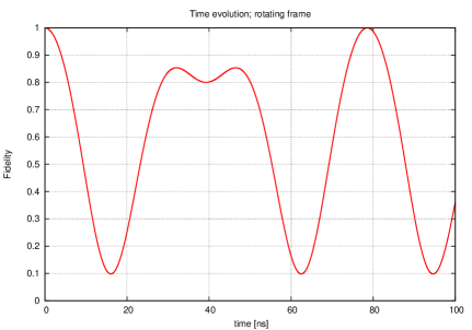
It turns out that is a very fast oscillating quantity, governed by the frequency 2​ω2πœ”2\omega. This less interesting β€˜free’ evolution can be eliminated exploiting the rotating frame, cf. Naus-stab . The fidelity in this rotating frame is obtained by replacing E16subscript𝐸16E_{16} by π’₯π’₯\mathcal{J} in (IV.1) and is depicted in figure (1) for two values of the exchange constant π’₯π’₯\mathcal{J}.

Refer to caption
Refer to caption
Figure 1: Fidelities: top π’₯=π’₯absent\mathcal{J}= 80 MHz; low π’₯=π’₯absent\mathcal{J}= 800 MHz; note the timescales.

Changing the vales of π’₯π’₯\mathcal{J} merely changes the timescale: stronger coupling causes a faster decrease in fidelity.

Analogous computations yield the probabilities to obtain the other possible measurement results:

p↓↑=p↑↓=118​[1βˆ’cos⁑{(E14βˆ’E8)​t}]subscript𝑝↓absent↑subscript𝑝↑absent↓118delimited-[]1subscript𝐸14subscript𝐸8𝑑p_{\downarrow\uparrow}=p_{\uparrow\downarrow}=\tfrac{1}{18}\left[1-\cos{\left\{(E_{14}-E_{8})t\right\}}\right] (28)

and

p↑↑=Ξ²βˆ—β€‹(t)​β​(t),subscript𝑝↑absent↑superscript𝛽𝑑𝛽𝑑p_{\uparrow\uparrow}=\beta^{*}(t)\beta(t), (29)

with

β​(t)=12​2​(13​eβˆ’i​E8​tβˆ’12​eβˆ’i​E10​t+16​eβˆ’i​E14​t).𝛽𝑑12213superscript𝑒𝑖subscript𝐸8𝑑12superscript𝑒𝑖subscript𝐸10𝑑16superscript𝑒𝑖subscript𝐸14𝑑\beta(t)=\tfrac{1}{2}\sqrt{2}\left(\tfrac{1}{3}e^{-iE_{8}t}-\tfrac{1}{2}e^{-iE_{10}t}+\tfrac{1}{6}e^{-iE_{14}t}\right). (30)

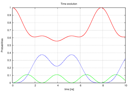
Note that the sum of the probabilities indeed is equal to one for all t𝑑t. They are shown in figure (2).

Refer to caption
Refer to caption
Figure 2: Probabilities: p↓↓subscript𝑝↓absent↓p_{\downarrow\downarrow} red, p↑↓=p↓↑subscript𝑝↑absent↓subscript𝑝↓absent↑p_{\uparrow\downarrow}=p_{\downarrow\uparrow} green, p↑↑subscript𝑝↑absent↑p_{\uparrow\uparrow} blue; top π’₯=π’₯absent\mathcal{J}= 80 MHz; low π’₯=π’₯absent\mathcal{J}= 800 MHz; note the timescales.

Again we note that altering the value of π’₯π’₯\mathcal{J} changes the timescale; in this case for the varying probabilities.

IV.2 Bell state |Ψ+⟩ketsuperscriptΨ|\Psi^{+}\rangle

We repeat these computations for the other Bell states as well. First, we consider |Ξ¨+⟩ketsuperscriptΞ¨|\Psi^{+}\rangle which corresponds to B+=1,A+=Aβˆ’=Bβˆ’=0formulae-sequencesubscript𝐡1subscript𝐴subscript𝐴subscript𝐡0B_{+}=1,A_{+}=A_{-}=B_{-}=0 in (18). Initial and time-evolved state follow respectively as

|ψ+⟩=βˆ’12​2​|e6βŸ©βˆ’16​6​|e8⟩+13​3​|e14⟩ketsuperscriptπœ“122ketsubscript𝑒6166ketsubscript𝑒8133ketsubscript𝑒14|\psi^{+}\rangle=-\tfrac{1}{2}\sqrt{2}|e_{6}\rangle-\tfrac{1}{6}\sqrt{6}|e_{8}\rangle+\tfrac{1}{3}\sqrt{3}|e_{14}\rangle (31)

and

|ψ+​(t)⟩ketsuperscriptπœ“π‘‘\displaystyle|\psi^{+}(t)\rangle =\displaystyle= βˆ’12​2​eβˆ’i​E6​t​|e6βŸ©βˆ’16​6​eβˆ’i​E8​t​|e8⟩122superscript𝑒𝑖subscript𝐸6𝑑ketsubscript𝑒6166superscript𝑒𝑖subscript𝐸8𝑑ketsubscript𝑒8\displaystyle-\tfrac{1}{2}\sqrt{2}e^{-iE_{6}t}|e_{6}\rangle-\tfrac{1}{6}\sqrt{6}e^{-iE_{8}t}|e_{8}\rangle (32)
+\displaystyle+ 13​3​eβˆ’i​E14​t​|e14⟩.133superscript𝑒𝑖subscript𝐸14𝑑ketsubscript𝑒14\displaystyle\tfrac{1}{3}\sqrt{3}e^{-iE_{14}t}|e_{14}\rangle.

Using the measurement operator corresponding to the β€˜correct result’ yields

P↓↑​|ψ+​(t)⟩=γ​(t)​|T0[12]βŸ©βŠ—(|T0[a​b]βŸ©βˆ’|S[a​b]⟩),subscript𝑃↓absent↑ketsuperscriptπœ“π‘‘tensor-product𝛾𝑑ketsuperscriptsubscript𝑇0delimited-[]12ketsuperscriptsubscript𝑇0delimited-[]π‘Žπ‘ketsuperscript𝑆delimited-[]π‘Žπ‘P_{\downarrow\uparrow}|\psi^{+}(t)\rangle=\gamma(t)|T_{0}^{[12]}\rangle\otimes(|T_{0}^{[ab]}\rangle-|S^{[ab]}\rangle), (33)

a product state, with time dependence

γ​(t)=12​eβˆ’i​E6​t+16​eβˆ’i​E8​t+13​eβˆ’i​E14​t.𝛾𝑑12superscript𝑒𝑖subscript𝐸6𝑑16superscript𝑒𝑖subscript𝐸8𝑑13superscript𝑒𝑖subscript𝐸14𝑑\gamma(t)=\tfrac{1}{2}e^{-iE_{6}t}+\tfrac{1}{6}e^{-iE_{8}t}+\tfrac{1}{3}e^{-iE_{14}t}. (34)

This leads to the probability

p↓↑=Ξ³βˆ—β€‹(t)​γ​(t).subscript𝑝↓absent↑superscript𝛾𝑑𝛾𝑑p_{\downarrow\uparrow}=\gamma^{*}(t)\gamma(t). (35)

The resulting two-qubit state

|Ψ​(t)⟩=γ​(t)p↓↑​|T012]⟩|\Psi(t)\rangle=\frac{\gamma(t)}{\sqrt{p_{\downarrow\uparrow}}}|T_{0}^{12]}\rangle (36)

has fidelity one with respect to the target state |Ψ+⟩ketsuperscriptΨ|\Psi^{+}\rangle.

The probabilities for obtaining the results which would be interpreted as error detection follow as

p↓↓=p↑↑=19​[1βˆ’cos⁑{(E14βˆ’E8)​t}]subscript𝑝↓absent↓subscript𝑝↑absent↑19delimited-[]1subscript𝐸14subscript𝐸8𝑑p_{\downarrow\downarrow}=p_{\uparrow\uparrow}=\tfrac{1}{9}\left[1-\cos{\left\{(E_{14}-E_{8})t\right\}}\right] (37)

and

p↑↓=ΞΌβˆ—β€‹(t)​μ​(t),subscript𝑝↑absent↓superscriptπœ‡π‘‘πœ‡π‘‘p_{\uparrow\downarrow}=\mu^{*}(t)\mu(t), (38)

with

μ​(t)=βˆ’12​eβˆ’i​E6​t+16​eβˆ’i​E8​t+13​eβˆ’i​E14​t.πœ‡π‘‘12superscript𝑒𝑖subscript𝐸6𝑑16superscript𝑒𝑖subscript𝐸8𝑑13superscript𝑒𝑖subscript𝐸14𝑑\mu(t)=-\tfrac{1}{2}e^{-iE_{6}t}+\tfrac{1}{6}e^{-iE_{8}t}+\tfrac{1}{3}e^{-iE_{14}t}. (39)

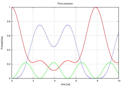
The various probabilities, indeed adding up to one, are shown in figure (3). Once more, we see time-scaling with the coupling strength.

Refer to caption
Refer to caption
Figure 3: Probabilities: p↓↑subscript𝑝↓absent↑p_{\downarrow\uparrow} red, p↑↑=p↓↓subscript𝑝↑absent↑subscript𝑝↓absent↓p_{\uparrow\uparrow}=p_{\downarrow\downarrow} green, p↑↓subscript𝑝↑absent↓p_{\uparrow\downarrow} blue; top π’₯=π’₯absent\mathcal{J}= 80 MHz; low π’₯=π’₯absent\mathcal{J}= 800 MHz; note the timescales.

IV.3 Bell state |Ξ¦βˆ’βŸ©ketsuperscriptΞ¦|\Phi^{-}\rangle

Next, we take Aβˆ’=1,A+=Bβˆ’=B+=0formulae-sequencesubscript𝐴1subscript𝐴subscript𝐡subscript𝐡0A_{-}=1,A_{+}=B_{-}=B_{+}=0 in (18) corresponding to the two-qubit state |Ξ¦βˆ’βŸ©ketsuperscriptΞ¦|\Phi^{-}\rangle. We immediately proceed to the state after time-evolution:

|Ο•βˆ’β€‹(t)⟩ketsuperscriptitalic-ϕ𝑑\displaystyle|\phi^{-}(t)\rangle =\displaystyle= βˆ’12​eβˆ’i​E5​t​|e5⟩+12​eβˆ’i​E7​t​|e7βŸ©βˆ’14​2​eβˆ’i​E9​t​|e9⟩12superscript𝑒𝑖subscript𝐸5𝑑ketsubscript𝑒512superscript𝑒𝑖subscript𝐸7𝑑ketsubscript𝑒7142superscript𝑒𝑖subscript𝐸9𝑑ketsubscript𝑒9\displaystyle-\tfrac{1}{2}e^{-iE_{5}t}|e_{5}\rangle+\tfrac{1}{2}e^{-iE_{7}t}|e_{7}\rangle-\tfrac{1}{4}\sqrt{2}e^{-iE_{9}t}|e_{9}\rangle (40)
βˆ’\displaystyle- 14​2​eβˆ’i​E11​t​|e11βŸ©βˆ’14​2​eβˆ’i​E13​t​|e13⟩142superscript𝑒𝑖subscript𝐸11𝑑ketsubscript𝑒11142superscript𝑒𝑖subscript𝐸13𝑑ketsubscript𝑒13\displaystyle\tfrac{1}{4}\sqrt{2}e^{-iE_{11}t}|e_{11}\rangle-\tfrac{1}{4}\sqrt{2}e^{-iE_{13}t}|e_{13}\rangle
+\displaystyle+ 14​2​eβˆ’i​E14​t​|e14⟩.142superscript𝑒𝑖subscript𝐸14𝑑ketsubscript𝑒14\displaystyle\tfrac{1}{4}\sqrt{2}e^{-iE_{14}t}|e_{14}\rangle.

Operating with the appropriate measurement operator for the β€˜correct result’ gives

P↑↓​|Ο•βˆ’β€‹(t)⟩subscript𝑃↑absent↓ketsuperscriptitalic-ϕ𝑑\displaystyle P_{\uparrow\downarrow}|\phi^{-}(t)\rangle =\displaystyle= βˆ’18​2​{Ο‡+​(t)​|T+[12]βŸ©βˆ’Ο‡βˆ’β€‹(t)​|Tβˆ’[12]⟩}182subscriptπœ’π‘‘ketsuperscriptsubscript𝑇delimited-[]12subscriptπœ’π‘‘ketsuperscriptsubscript𝑇delimited-[]12\displaystyle-\tfrac{1}{8}\sqrt{2}\left\{\chi_{+}(t)|T_{+}^{[12]}\rangle-\chi_{-}(t)|T_{-}^{[12]}\rangle\right\} (41)
βŠ—tensor-product\displaystyle\otimes (|T0[a​b]⟩+|S[a​b]⟩),ketsuperscriptsubscript𝑇0delimited-[]π‘Žπ‘ketsuperscript𝑆delimited-[]π‘Žπ‘\displaystyle\left(|T_{0}^{[ab]}\rangle+|S^{[ab]}\rangle\right),

with the functions

Ο‡+​(t)subscriptπœ’π‘‘\displaystyle\chi_{+}(t) =\displaystyle= 2​eβˆ’i​E5​t+eβˆ’i​E9​t+eβˆ’i​E13​t,2superscript𝑒𝑖subscript𝐸5𝑑superscript𝑒𝑖subscript𝐸9𝑑superscript𝑒𝑖subscript𝐸13𝑑\displaystyle 2e^{-iE_{5}t}+e^{-iE_{9}t}+e^{-iE_{13}t},
Ο‡βˆ’β€‹(t)subscriptπœ’π‘‘\displaystyle\chi_{-}(t) =\displaystyle= 2​eβˆ’i​E7​t+eβˆ’i​E11​t+eβˆ’i​E15​t.2superscript𝑒𝑖subscript𝐸7𝑑superscript𝑒𝑖subscript𝐸11𝑑superscript𝑒𝑖subscript𝐸15𝑑\displaystyle 2e^{-iE_{7}t}+e^{-iE_{11}t}+e^{-iE_{15}t}. (42)

The probability to get the measurement result ↑,↓↑↓\uparrow,\downarrow follows as

p↑↓=132​(Ο‡+βˆ—β€‹(t)​χ+​(t)+Ο‡βˆ’βˆ—β€‹(t)β€‹Ο‡βˆ’β€‹(t)).subscript𝑝↑absent↓132subscriptsuperscriptπœ’π‘‘subscriptπœ’π‘‘subscriptsuperscriptπœ’π‘‘subscriptπœ’π‘‘p_{\uparrow\downarrow}=\tfrac{1}{32}\left(\chi^{*}_{+}(t)\chi_{+}(t)+\chi^{*}_{-}(t)\chi_{-}(t)\right). (43)

After factoring out the ancilla states we obtain for the corresponding fidelilty

F=18​[(Ο‡+​(t)+Ο‡βˆ’β€‹(t))​(Ο‡+βˆ—β€‹(t)+Ο‡βˆ’βˆ—β€‹(t))/p↑↓]1/2.𝐹18superscriptdelimited-[]subscriptπœ’π‘‘subscriptπœ’π‘‘subscriptsuperscriptπœ’π‘‘subscriptsuperscriptπœ’π‘‘subscript𝑝↑absent↓12F=\tfrac{1}{8}\left[\left(\chi_{+}(t)+\chi_{-}(t)\right)\left(\chi^{*}_{+}(t)+\chi^{*}_{-}(t)\right)/p_{\uparrow\downarrow}\right]^{1/2}. (44)

This fidelity also oscillates very fast. This is a result of the interference terms Ο‡+βˆ—β€‹Ο‡βˆ’superscriptsubscriptπœ’subscriptπœ’\chi_{+}^{*}\chi_{-} and Ο‡βˆ’βˆ—β€‹Ο‡+superscriptsubscriptπœ’superscriptπœ’\chi_{-}^{*}\chi^{+} which have a frequency of 2​ω2πœ”2\omega. In the rotating frame of the qubits it vanishes. The resulting fidelity in this frame is equal one for all times since in the rotating frame

χ±​(t)β†’Ο‡~±​(t)=eΒ±i​ω​t​χ±​(t)β†’subscriptπœ’plus-or-minus𝑑subscript~πœ’plus-or-minus𝑑superscript𝑒plus-or-minusπ‘–πœ”π‘‘subscriptπœ’plus-or-minus𝑑\chi_{\pm}(t)\rightarrow\tilde{\chi}_{\pm}(t)=e^{\pm i\omega t}\chi_{\pm}(t) (45)

and Ο‡~+​(t)=Ο‡~βˆ’β€‹(t)subscript~πœ’π‘‘subscript~πœ’π‘‘\tilde{\chi}_{+}(t)=\tilde{\chi}_{-}(t). As a consequence, we obtain

F=18​[64​p↑↓/p↑↓]1/2=1,𝐹18superscriptdelimited-[]64subscript𝑝↑absent↓subscript𝑝↑absent↓121F=\tfrac{1}{8}\left[64p_{\uparrow\downarrow}/p_{\uparrow\downarrow}\right]^{1/2}=1, (46)

which may be somewhat surprising.

The other, β€˜error detection’ probabilities can be calculated analogously. We get the results

p↓↓subscript𝑝↓absent↓\displaystyle p_{\downarrow\downarrow} =\displaystyle= 18​[1βˆ’cos⁑{(E15βˆ’E11)​t}],18delimited-[]1subscript𝐸15subscript𝐸11𝑑\displaystyle\tfrac{1}{8}\left[1-\cos{\left\{(E_{15}-E_{11})t\right\}}\right],
p↑↑subscript𝑝↑absent↑\displaystyle p_{\uparrow\uparrow} =\displaystyle= 18​[1βˆ’cos⁑{(E13βˆ’E9)​t}],18delimited-[]1subscript𝐸13subscript𝐸9𝑑\displaystyle\tfrac{1}{8}\left[1-\cos{\left\{(E_{13}-E_{9})t\right\}}\right],
p↓↑subscript𝑝↓absent↑\displaystyle p_{\downarrow\uparrow} =\displaystyle= 132​(Ξ½+βˆ—β€‹(t)​ν+​(t)+Ξ½βˆ’βˆ—β€‹(t)β€‹Ξ½βˆ’β€‹(t)),132subscriptsuperscriptπœˆπ‘‘subscriptπœˆπ‘‘subscriptsuperscriptπœˆπ‘‘subscriptπœˆπ‘‘\displaystyle\tfrac{1}{32}\left(\nu^{*}_{+}(t)\nu_{+}(t)+\nu^{*}_{-}(t)\nu_{-}(t)\right), (47)

where we have defined

Ξ½+​(t)subscriptπœˆπ‘‘\displaystyle\nu_{+}(t) =\displaystyle= 2​eβˆ’i​E5​tβˆ’eβˆ’i​E9​tβˆ’eβˆ’i​E13​t,2superscript𝑒𝑖subscript𝐸5𝑑superscript𝑒𝑖subscript𝐸9𝑑superscript𝑒𝑖subscript𝐸13𝑑\displaystyle 2e^{-iE_{5}t}-e^{-iE_{9}t}-e^{-iE_{13}t},
Ξ½βˆ’β€‹(t)subscriptπœˆπ‘‘\displaystyle\nu_{-}(t) =\displaystyle= 2​eβˆ’i​E7​tβˆ’eβˆ’i​E11​tβˆ’eβˆ’i​E15​t.2superscript𝑒𝑖subscript𝐸7𝑑superscript𝑒𝑖subscript𝐸11𝑑superscript𝑒𝑖subscript𝐸15𝑑\displaystyle 2e^{-iE_{7}t}-e^{-iE_{11}t}-e^{-iE_{15}t}. (48)

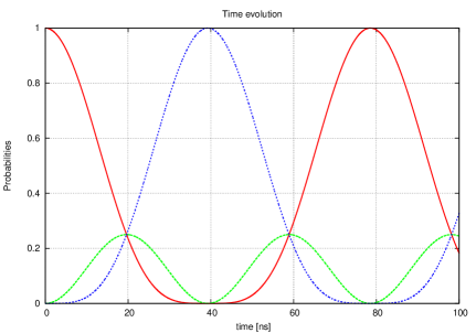
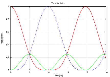
From the eigenenergies (II) it becomes clear that p↓↓=p↑↑subscript𝑝↓absent↓subscript𝑝↑absent↑p_{\downarrow\downarrow}=p_{\uparrow\uparrow}. Figure (4) depicts the calculated probabilities. We again get time-scaling with the coupling strength.
Refer to caption
Refer to caption
Figure 4: Probabilities: p↑↓subscript𝑝↑absent↓p_{\uparrow\downarrow} red, p↑↑=p↓↓subscript𝑝↑absent↑subscript𝑝↓absent↓p_{\uparrow\uparrow}=p_{\downarrow\downarrow} green, p↓↑subscript𝑝↓absent↑p_{\downarrow\uparrow} blue; top π’₯=π’₯absent\mathcal{J}= 80 MHz; low π’₯=π’₯absent\mathcal{J}= 800 MHz; note the timescales.

IV.4 Bell state |Ξ¨βˆ’βŸ©ketsuperscriptΞ¨|\Psi^{-}\rangle

This last case corresponds to Bβˆ’=1,A+=Aβˆ’=B+=0formulae-sequencesubscript𝐡1subscript𝐴subscript𝐴subscript𝐡0B_{-}=1,A_{+}=A_{-}=B_{+}=0 in (18); it actually is the simplest one because the initial four qubit state equals a basis state. Explicity we obtain

|Οˆβˆ’βŸ©ketsubscriptπœ“\displaystyle|\psi_{-}\rangle =\displaystyle= βˆ’|e2⟩,ketsubscript𝑒2\displaystyle-|e_{2}\rangle,
|Οˆβˆ’β€‹(t)⟩ketsubscriptπœ“π‘‘\displaystyle|\psi_{-}(t)\rangle =\displaystyle= βˆ’eβˆ’i​E2​t​|e2⟩,superscript𝑒𝑖subscript𝐸2𝑑ketsubscript𝑒2\displaystyle-e^{-iE_{2}t}|e_{2}\rangle,
P↑↑​|Οˆβˆ’β€‹(t)⟩subscript𝑃↑absent↑ketsubscriptπœ“π‘‘\displaystyle P_{\uparrow\uparrow}|\psi_{-}(t)\rangle =\displaystyle= βˆ’eβˆ’i​E2​t​|S[12]βŸ©βŠ—|T+[a​b]⟩tensor-productsuperscript𝑒𝑖subscript𝐸2𝑑ketsuperscript𝑆delimited-[]12ketsuperscriptsubscript𝑇delimited-[]π‘Žπ‘\displaystyle-e^{-iE_{2}t}|S^{[12]}\rangle\otimes|T_{+}^{[ab]}\rangle (49)

and the concomitant trivial probabilities

p↑↑=1,p↑↓=p↓↑=p↓↓=0.formulae-sequencesubscript𝑝↑absent↑1subscript𝑝↑absent↓subscript𝑝↓absent↑subscript𝑝↓absent↓0p_{\uparrow\uparrow}=1,\quad p_{\uparrow\downarrow}=p_{\downarrow\uparrow}=p_{\downarrow\downarrow}=0. (50)

After factoring out the ancillas state, the two-qubit state is -up to a phase- equal to the target state. As a consequence, the fidelity is equal to one. The unitary evolution has no negative impact on the ideal probabilities and fidelity for this particular Bell state.

V Quantum gates by unitary evolution

The obtained results show that the probabilities which were initially one, first decrease but after a time t~~𝑑\tilde{t} again become equal to one. For the Bell state |Ξ¦βˆ’βŸ©ketsuperscriptΞ¦|\Phi^{-}\rangle, we note that for t=t~/2𝑑~𝑑2t=\tilde{t}/2 the up-down probability (initially one) becomes zero, whereas the down-up probability equals one. This opens the possibility for two-qubit gates, that is an operation on the data qubits, which can be verified by measuring the ancillas without affecting the state of the data qubits. The time t~~𝑑\tilde{t} follows from

π’₯​t~=2​πast~=2​ππ’₯.formulae-sequenceπ’₯~𝑑2πœ‹as~𝑑2πœ‹π’₯\mathcal{J}\tilde{t}=2\pi\quad\text{as}\quad\tilde{t}=\frac{2\pi}{\mathcal{J}}. (51)

In order to address two-qubit gates in the four-qubit system we continue the analysis started above. To this end, we also need the computational basis. For two qubits we define the basis states |ck⟩,k=1,2,3,4formulae-sequenceketsubscriptπ‘π‘˜π‘˜1234|c_{k}\rangle,k=1,2,3,4 as the common computational states

|c1⟩=|β†“β†“βŸ©,|c2⟩=|β†“β†‘βŸ©,|c3⟩=|β†‘β†“βŸ©,|c4⟩=|β†‘β†‘βŸ©.|c_{1}\rangle=|\downarrow\,\downarrow\,\rangle,|c_{2}\rangle=|\downarrow\,\uparrow\,\rangle,|c_{3}\rangle=|\,\uparrow\,\downarrow\,\rangle,|c_{4}\rangle=|\,\uparrow\,\uparrow\,\rangle. (52)

The computational states for four qubits are the product states

|ck​l⟩=|ck[12]βŸ©βŠ—|cl[a​b]⟩,k,l=1,2,3,4.formulae-sequenceketsubscriptπ‘π‘˜π‘™tensor-productketsuperscriptsubscriptπ‘π‘˜delimited-[]12ketsuperscriptsubscript𝑐𝑙delimited-[]π‘Žπ‘π‘˜π‘™1234|c_{kl}\rangle=|c_{k}^{[12]}\rangle\otimes|c_{l}^{[ab]}\rangle,\quad k,l=1,2,3,4. (53)

We relabel the ancilla measurement operators (20) also as Plsubscript𝑃𝑙P_{l} and rewrite these as

Pl[a​b]=ℐ12βŠ—|cl[a​b]βŸ©β€‹βŸ¨cl[a​b]|=βˆ‘j=14|cj​lβŸ©β€‹βŸ¨cj​l|.superscriptsubscript𝑃𝑙delimited-[]π‘Žπ‘tensor-productsuperscriptℐ12ketsuperscriptsubscript𝑐𝑙delimited-[]π‘Žπ‘brasuperscriptsubscript𝑐𝑙delimited-[]π‘Žπ‘superscriptsubscript𝑗14ketsubscript𝑐𝑗𝑙brasubscript𝑐𝑗𝑙P_{l}^{[ab]}=\mathcal{I}^{12}\otimes|c_{l}^{[ab]}\rangle\langle c_{l}^{[ab]}|=\sum_{j=1}^{4}|c_{jl}\rangle\langle c_{jl}|. (54)

The initial state is assumed to be the product state of a computational basis state of the ancillas, say |cn[a​b]⟩ketsuperscriptsubscript𝑐𝑛delimited-[]π‘Žπ‘|c_{n}^{[ab]}\rangle with fixed n𝑛n and a general two-data qubit state:

|ψ0⟩={βˆ‘m=14Ξ±m​|cm[12]⟩}βŠ—|cna​b⟩=βˆ‘m=14Ξ±m​|cm​n⟩.ketsubscriptπœ“0tensor-productsuperscriptsubscriptπ‘š14subscriptπ›Όπ‘šketsuperscriptsubscriptπ‘π‘šdelimited-[]12ketsuperscriptsubscriptπ‘π‘›π‘Žπ‘superscriptsubscriptπ‘š14subscriptπ›Όπ‘šketsubscriptπ‘π‘šπ‘›|\psi_{0}\rangle=\left\{\sum_{m=1}^{4}\alpha_{m}|c_{m}^{[12]}\rangle\right\}\otimes|c_{n}^{ab}\rangle=\sum_{m=1}^{4}\alpha_{m}|c_{mn}\rangle. (55)

After unitary evolution governed by the operator (19), the state is given by

|Οˆβ€‹(t)⟩=βˆ‘k=116βˆ‘m=14Ξ±mβ€‹βŸ¨ek|cm​nβŸ©β€‹eβˆ’i​Ek​t​|ek⟩.ketπœ“π‘‘superscriptsubscriptπ‘˜116superscriptsubscriptπ‘š14subscriptπ›Όπ‘šinner-productsubscriptπ‘’π‘˜subscriptπ‘π‘šπ‘›superscript𝑒𝑖subscriptπΈπ‘˜π‘‘ketsubscriptπ‘’π‘˜|\psi(t)\rangle=\sum_{k=1}^{16}\sum_{m=1}^{4}\alpha_{m}\langle e_{k}|c_{mn}\rangle e^{-iE_{k}t}|e_{k}\rangle. (56)

Applying the ancilla measurement operator Pl[a​b]subscriptsuperscript𝑃delimited-[]π‘Žπ‘π‘™P^{[ab]}_{l} to this state yields

Pl[a​b]​|Οˆβ€‹(t)⟩subscriptsuperscript𝑃delimited-[]π‘Žπ‘π‘™ketπœ“π‘‘\displaystyle P^{[ab]}_{l}|\psi(t)\rangle =\displaystyle= βˆ‘j=14βˆ‘m=14Ξ±m​Wj​lβˆ’m​n​(t)​|cj​l⟩superscriptsubscript𝑗14superscriptsubscriptπ‘š14subscriptπ›Όπ‘šsubscriptπ‘Šπ‘—π‘™π‘šπ‘›π‘‘ketsubscript𝑐𝑗𝑙\displaystyle\sum_{j=1}^{4}\sum_{m=1}^{4}\alpha_{m}W_{jl-mn}(t)|c_{jl}\rangle
=\displaystyle= {βˆ‘j=14βˆ‘m=14Ξ±m​Wj​lβˆ’m​n​(t)​|cj[12]⟩}βŠ—|cl[ab⟩,\displaystyle\left\{\sum_{j=1}^{4}\sum_{m=1}^{4}\alpha_{m}W_{jl-mn}(t)|c_{j}^{[12]}\rangle\right\}\otimes|c_{l}^{[ab}\rangle,

where we have defined

Wj​lβˆ’m​n​(t)=βˆ‘k=116⟨ek|cm​nβŸ©β€‹βŸ¨cj​l|ekβŸ©β€‹eβˆ’i​Ek​t.subscriptπ‘Šπ‘—π‘™π‘šπ‘›π‘‘superscriptsubscriptπ‘˜116inner-productsubscriptπ‘’π‘˜subscriptπ‘π‘šπ‘›inner-productsubscript𝑐𝑗𝑙subscriptπ‘’π‘˜superscript𝑒𝑖subscriptπΈπ‘˜π‘‘W_{jl-mn}(t)=\sum_{k=1}^{16}\langle e_{k}|c_{mn}\rangle\langle c_{jl}|e_{k}\rangle e^{-iE_{k}t}. (58)

Since the coefficients ⟨ek|cm​n⟩inner-productsubscriptπ‘’π‘˜subscriptπ‘π‘šπ‘›\langle e_{k}|c_{mn}\rangle are real, Wπ‘ŠW is symmetric: Wj​lβˆ’m​n​(t)=Wm​nβˆ’j​l​(t)subscriptπ‘Šπ‘—π‘™π‘šπ‘›π‘‘subscriptπ‘Šπ‘šπ‘›π‘—π‘™π‘‘W_{jl-mn}(t)=W_{mn-jl}(t). The measurement probabilities for obtaining the result l𝑙l follow as

pl​n​(t)=βˆ‘m=14βˆ‘mβ€²=14βˆ‘j=14Ξ±mβ€²βˆ—β€‹Ξ±m​Wj​lβˆ’m′​nβˆ—β€‹(t)​Wj​lβˆ’m​n​(t),subscript𝑝𝑙𝑛𝑑superscriptsubscriptπ‘š14superscriptsubscriptsuperscriptπ‘šβ€²14superscriptsubscript𝑗14subscriptsuperscript𝛼superscriptπ‘šβ€²subscriptπ›Όπ‘šsubscriptsuperscriptπ‘Šπ‘—π‘™superscriptπ‘šβ€²π‘›π‘‘subscriptπ‘Šπ‘—π‘™π‘šπ‘›π‘‘p_{ln}(t)=\sum_{m=1}^{4}\sum_{m^{\prime}=1}^{4}\sum_{j=1}^{4}\alpha^{*}_{m^{\prime}}\alpha_{m}W^{*}_{jl-m^{\prime}n}(t)W_{jl-mn}(t), (59)

where we have explicitly indicated the dependence on the initial ancillas state. Note the implicit dependence on the initial data qubit states. The corresponding amputated and normalized final data qubit state is obtained as

|ψl​n[12]​(t)⟩ketsuperscriptsubscriptπœ“π‘™π‘›delimited-[]12𝑑\displaystyle|\psi_{ln}^{[12]}(t)\rangle =\displaystyle= 1pl​nβ€‹βˆ‘j=14βˆ‘m=14Ξ±m​Wj​lβˆ’m​n​(t)​|cj[12]⟩1subscript𝑝𝑙𝑛superscriptsubscript𝑗14superscriptsubscriptπ‘š14subscriptπ›Όπ‘šsubscriptπ‘Šπ‘—π‘™π‘šπ‘›π‘‘ketsuperscriptsubscript𝑐𝑗delimited-[]12\displaystyle\frac{1}{\sqrt{p_{ln}}}\sum_{j=1}^{4}\sum_{m=1}^{4}\alpha_{m}W_{jl-mn}(t)|c_{j}^{[12]}\rangle (60)
=\displaystyle= βˆ‘j=14Ξ²j[l​n]​(t)​|cj[12]⟩,superscriptsubscript𝑗14subscriptsuperscript𝛽delimited-[]𝑙𝑛𝑗𝑑ketsuperscriptsubscript𝑐𝑗delimited-[]12\displaystyle\sum_{j=1}^{4}\beta^{[ln]}_{j}(t)|c_{j}^{[12]}\rangle,

with the functions

Ξ²j[l​n]​(t)=1pl​nβ€‹βˆ‘m=14Ξ±m​Wj​lβˆ’m​n​(t).subscriptsuperscript𝛽delimited-[]𝑙𝑛𝑗𝑑1subscript𝑝𝑙𝑛superscriptsubscriptπ‘š14subscriptπ›Όπ‘šsubscriptπ‘Šπ‘—π‘™π‘šπ‘›π‘‘\beta^{[ln]}_{j}(t)=\frac{1}{\sqrt{p_{ln}}}\sum_{m=1}^{4}\alpha_{m}W_{jl-mn}(t). (61)

Comparison of this final state and the initial one (55) suggest a linear relation between these states. Because of the abovementioned dependence of the probabilities on the coefficients Ξ±msubscriptπ›Όπ‘š\alpha_{m} this is, however, in general not true. The dependence only vanishes for zero probability which is not interesting and for the relevant case of probability one. If for an instant of time t~~𝑑\tilde{t} and a specific combination of l,n𝑙𝑛l,n

βˆ‘j=14Wj​lβˆ’m′​nβˆ—β€‹(t~)​Wj​lβˆ’m​n​(t~)=Ξ΄m​mβ€²,superscriptsubscript𝑗14subscriptsuperscriptπ‘Šπ‘—π‘™superscriptπ‘šβ€²π‘›~𝑑subscriptπ‘Šπ‘—π‘™π‘šπ‘›~𝑑subscriptπ›Ώπ‘šsuperscriptπ‘šβ€²\sum_{j=1}^{4}W^{*}_{jl-m^{\prime}n}(\tilde{t})W_{jl-mn}(\tilde{t})=\delta_{mm^{\prime}}, (62)

the probability becomes one

pl​n​(t~)=βˆ‘m=14βˆ‘mβ€²=14Ξ±mβ€²βˆ—β€‹Ξ±m​δm​mβ€²=βˆ‘m=14Ξ±mβˆ—β€‹Ξ±m=1.subscript𝑝𝑙𝑛~𝑑superscriptsubscriptπ‘š14superscriptsubscriptsuperscriptπ‘šβ€²14subscriptsuperscript𝛼superscriptπ‘šβ€²subscriptπ›Όπ‘šsubscriptπ›Ώπ‘šsuperscriptπ‘šβ€²superscriptsubscriptπ‘š14subscriptsuperscriptπ›Όπ‘šsubscriptπ›Όπ‘š1p_{ln}(\tilde{t})=\sum_{m=1}^{4}\sum_{m^{\prime}=1}^{4}\alpha^{*}_{m^{\prime}}\alpha_{m}\delta_{mm^{\prime}}=\sum_{m=1}^{4}\alpha^{*}_{m}\alpha_{m}=1. (63)

In fact, in the numerical implementation described below, we have found that the specific l,n𝑙𝑛l,n combinations are l=n𝑙𝑛l=n. Thus the latter two equations actually read

βˆ‘j=14Wj​lβˆ’m′​nβˆ—β€‹(t~)​Wj​lβˆ’m​n​(t~)=Ξ΄m​m′​δl​n,superscriptsubscript𝑗14subscriptsuperscriptπ‘Šπ‘—π‘™superscriptπ‘šβ€²π‘›~𝑑subscriptπ‘Šπ‘—π‘™π‘šπ‘›~𝑑subscriptπ›Ώπ‘šsuperscriptπ‘šβ€²subscript𝛿𝑙𝑛\sum_{j=1}^{4}W^{*}_{jl-m^{\prime}n}(\tilde{t})W_{jl-mn}(\tilde{t})=\delta_{mm^{\prime}}\delta_{ln}, (64)

and

pl​n​(t~)=Ξ΄l​nβ€‹βˆ‘m=14βˆ‘mβ€²=14Ξ±mβ€²βˆ—β€‹Ξ±m​δm​mβ€²=Ξ΄l​nβ€‹βˆ‘m=14Ξ±mβˆ—β€‹Ξ±m=Ξ΄l​n.subscript𝑝𝑙𝑛~𝑑subscript𝛿𝑙𝑛superscriptsubscriptπ‘š14superscriptsubscriptsuperscriptπ‘šβ€²14subscriptsuperscript𝛼superscriptπ‘šβ€²subscriptπ›Όπ‘šsubscriptπ›Ώπ‘šsuperscriptπ‘šβ€²subscript𝛿𝑙𝑛superscriptsubscriptπ‘š14subscriptsuperscriptπ›Όπ‘šsubscriptπ›Όπ‘šsubscript𝛿𝑙𝑛p_{ln}(\tilde{t})=\delta_{ln}\sum_{m=1}^{4}\sum_{m^{\prime}=1}^{4}\alpha^{*}_{m^{\prime}}\alpha_{m}\delta_{mm^{\prime}}=\delta_{ln}\sum_{m=1}^{4}\alpha^{*}_{m}\alpha_{m}=\delta_{ln}. (65)

It indeed implies that the coefficients Ξ²j[n​n]​(t~)superscriptsubscript𝛽𝑗delimited-[]𝑛𝑛~𝑑\beta_{j}^{[nn]}(\tilde{t}) depend linearly on the initial ones Ξ±msubscriptπ›Όπ‘š\alpha_{m}. Consequently, we obtain a final two-qubit state which follows as a gate operation on the initial one

|ψn​n[12]​(t~)⟩ketsuperscriptsubscriptπœ“π‘›π‘›delimited-[]12~𝑑\displaystyle|\psi_{nn}^{[12]}(\tilde{t})\rangle =\displaystyle= βˆ‘j=14Ξ²j[n​n]​(t~)​|cj[12]⟩superscriptsubscript𝑗14subscriptsuperscript𝛽delimited-[]𝑛𝑛𝑗~𝑑ketsuperscriptsubscript𝑐𝑗delimited-[]12\displaystyle\sum_{j=1}^{4}\beta^{[nn]}_{j}(\tilde{t})|c_{j}^{[12]}\rangle (66)
=\displaystyle= βˆ‘j=14βˆ‘m=14Ξ±m​Wj​nβˆ’m​n​(t~)​|cj[12]⟩.superscriptsubscript𝑗14superscriptsubscriptπ‘š14subscriptπ›Όπ‘šsubscriptπ‘Šπ‘—π‘›π‘šπ‘›~𝑑ketsuperscriptsubscript𝑐𝑗delimited-[]12\displaystyle\sum_{j=1}^{4}\sum_{m=1}^{4}\alpha_{m}W_{jn-mn}(\tilde{t})|c_{j}^{[12]}\rangle.

In matrix form, the gate is explicitly given by

Ξ²j[n​n]​(t~)=βˆ‘m=14Wj​nβˆ’m​n​(t~)​αm.subscriptsuperscript𝛽delimited-[]𝑛𝑛𝑗~𝑑superscriptsubscriptπ‘š14subscriptπ‘Šπ‘—π‘›π‘šπ‘›~𝑑subscriptπ›Όπ‘š\beta^{[nn]}_{j}(\tilde{t})=\sum_{m=1}^{4}W_{jn-mn}(\tilde{t})\alpha_{m}. (67)

Unitarity of the gate, or matrix, is guaranteed by the constraints (62,64). Note that, for an arbitrary initial data qubit state, the probability only becomes one for obtaining the same ancilla spin values as initialized. In situations where the data qubits are initialized in a specific computational state, other measurement results, e.g. ↓↑↓absent↑\downarrow\uparrow instead of ↑↓↑absent↓\uparrow\downarrow, with probability one also have appeared. It does not simultaneously happen, however, for all four initial computational data qubit states and, consequently, no unitary operation is effectuated.

In the way described above, four unitary gates are in principle obtained by evolution and projection at t=t~𝑑~𝑑t=\tilde{t}:

Uj​mn​(t~)=Wj​nβˆ’m​n​(t~),n=1,2,3,4.formulae-sequencesuperscriptsubscriptπ‘ˆπ‘—π‘šπ‘›~𝑑subscriptπ‘Šπ‘—π‘›π‘šπ‘›~𝑑𝑛1234U_{jm}^{n}(\tilde{t})=W_{jn-mn}(\tilde{t}),\quad n=1,2,3,4. (68)

It will further be analyzed numerically as well as analytically; these methods have turned out to be complementary for obtaining the results.

V.1 Implementation

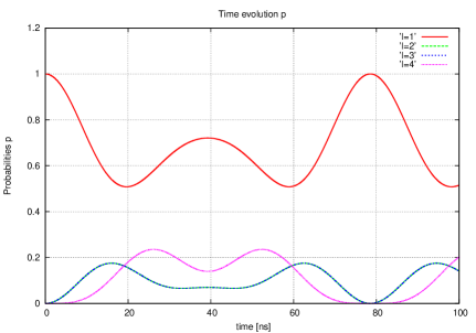
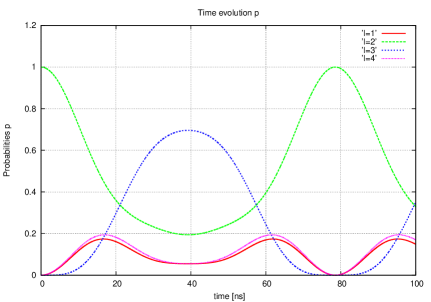
We have implemented the formalism in a computer program. To compute the quantities Wj​lβˆ’m​n​(t)subscriptπ‘Šπ‘—π‘™π‘šπ‘›π‘‘W_{jl-mn}(t), all the necessary ingredients have been obtained analytically. These are the eigenstates |ek⟩ketsubscriptπ‘’π‘˜|e_{k}\rangle and the concomitant energy eigenvalues EksubscriptπΈπ‘˜E_{k} presented in section II. Additionally, the basis transformation ⟨ek|cm​n⟩inner-productsubscriptπ‘’π‘˜subscriptπ‘π‘šπ‘›\langle e_{k}|c_{mn}\rangle is needed. Since the eigenstates are expressed in singlet-triplet basis states -for data and ancilla qubits- it can be computed using the transformation between singlet-triplet and computational basis. Next the measurement probabilities (59) are calculated for given initial data qubit state, i.e., given coefficients Ξ±msubscriptπ›Όπ‘š\alpha_{m}. They can be chosen by hand or randomly generated by a random-number generator for a given probability density function. We have chosen a uniform distribution around zero for real as well as imaginary parts. Of course, the state has then to be normalized. The resulting measurement probabilities for all l,n𝑙𝑛l,n combinations are plotted as a function of time and the instant of time where a probability becomes one is identified. Indeed we find that for l=n𝑙𝑛l=n this instant of time is given by t~=2​ππ’₯~𝑑2πœ‹π’₯\tilde{t}=\frac{2\pi}{\mathcal{J}}. Figure (5) shows the measurement probabilities for n=1𝑛1n=1 and n=2𝑛2n=2 and all l=1,2,3,4𝑙1234l=1,2,3,4. It explicitly illustrates the already mentioned results. The initial data qubit state is randomly selected in this example.
Refer to caption
Refer to caption
Figure 5: Probabilities: π’₯=π’₯absent\mathcal{J}= 80 MHz; top n=1𝑛1n=1, low n=2𝑛2n=2

The resulting gates explicitly read

U1superscriptπ‘ˆ1\displaystyle U^{1} =\displaystyle= (e4​π​i​ωπ’₯0000e2​π​i​ωπ’₯0000e2​π​i​ωπ’₯00001),matrixsuperscript𝑒4πœ‹π‘–πœ”π’₯0000superscript𝑒2πœ‹π‘–πœ”π’₯0000superscript𝑒2πœ‹π‘–πœ”π’₯00001\displaystyle\begin{pmatrix}e^{\frac{4\pi i\omega}{\mathcal{J}}}&0&0&0\\ 0&e^{\frac{2\pi i\omega}{\mathcal{J}}}&0&0\\ 0&0&e^{\frac{2\pi i\omega}{\mathcal{J}}}&0\\ 0&0&0&1\end{pmatrix},
U2superscriptπ‘ˆ2\displaystyle U^{2} =\displaystyle= eβˆ’2​π​i​ωπ’₯​U1,U3=eβˆ’2​π​i​ωπ’₯​U2,superscript𝑒2πœ‹π‘–πœ”π’₯superscriptπ‘ˆ1superscriptπ‘ˆ3superscript𝑒2πœ‹π‘–πœ”π’₯superscriptπ‘ˆ2\displaystyle e^{-\frac{2\pi i\omega}{\mathcal{J}}}U^{1},\quad U^{3}=e^{-\frac{2\pi i\omega}{\mathcal{J}}}U^{2},
U4superscriptπ‘ˆ4\displaystyle U^{4} =\displaystyle= eβˆ’2​π​i​ωπ’₯​U3.superscript𝑒2πœ‹π‘–πœ”π’₯superscriptπ‘ˆ3\displaystyle e^{-\frac{2\pi i\omega}{\mathcal{J}}}U^{3}. (69)

These are four, phase-equivalent phase gates.

V.2 Analytical construction

With some effort, these gates can be obtained analytically as well. The inititial state is completely specified as a product state of a computational data qubit state and a computational ancilla qubit state. It is rewritten in terms of eigenstates of the Hamiltonian in order to construct the time-evoluted state. Next the time is identified upon a measurement yields a result with probability one and the resulting two-data-qubit state is identified. Let is explicitly demonstrate this for the initial state

|Ο•0⟩=|β†“β†“βŸ©βŠ—|β†“β†‘βŸ©,|\phi_{0}\rangle=|\downarrow\,\downarrow\,\rangle\otimes|\downarrow\,\uparrow\,\rangle, (70)

which reads in terms of singlet-triplet basis states as

|Ο•0⟩=12​2​|Tβˆ’[12]βŸ©β€‹(|T0[a​b]βŸ©βˆ’|S[a​b]⟩).ketsubscriptitalic-Ο•0122ketsuperscriptsubscript𝑇delimited-[]12ketsuperscriptsubscript𝑇0delimited-[]π‘Žπ‘ketsuperscript𝑆delimited-[]π‘Žπ‘|\phi_{0}\rangle=\tfrac{1}{2}\sqrt{2}|T_{-}^{[12]}\rangle\left(|T_{0}^{[ab]}\rangle-|S^{[ab]}\rangle\right). (71)

Rewriting it as a linear combination of eigenstates yields

|Ο•0⟩=βˆ’12​(|e11βŸ©βˆ’|e15⟩+2​|e7⟩).ketsubscriptitalic-Ο•012ketsubscript𝑒11ketsubscript𝑒152ketsubscript𝑒7|\phi_{0}\rangle=-\tfrac{1}{2}\left(|e_{11}\rangle-|e_{15}\rangle+\sqrt{2}|e_{7}\rangle\right). (72)

As a consequence, after time evolution we get

|ϕ​(t)⟩=βˆ’12​(eβˆ’i​E11​t​|e11βŸ©βˆ’eβˆ’i​E15​t​|e15⟩+2​ei​E7​t​|e7⟩).ketitalic-ϕ𝑑12superscript𝑒𝑖subscript𝐸11𝑑ketsubscript𝑒11superscript𝑒𝑖subscript𝐸15𝑑ketsubscript𝑒152superscript𝑒𝑖subscript𝐸7𝑑ketsubscript𝑒7|\phi(t)\rangle=-\tfrac{1}{2}\left(e^{-iE_{11}t}|e_{11}\rangle-e^{-iE_{15}t}|e_{15}\rangle+\sqrt{2}e^{iE_{7}t}|e_{7}\rangle\right). (73)

Now it is readily checked that

|ϕ​(t~)⟩ketitalic-Ο•~𝑑\displaystyle|\phi(\tilde{t})\rangle =\displaystyle= βˆ’12​(ei​ω​t~​|e11βŸ©βˆ’ei​ω​t~​|e15⟩+2​ei​ω​t~​|e7⟩)12superscriptπ‘’π‘–πœ”~𝑑ketsubscript𝑒11superscriptπ‘’π‘–πœ”~𝑑ketsubscript𝑒152superscriptπ‘’π‘–πœ”~𝑑ketsubscript𝑒7\displaystyle-\tfrac{1}{2}\left(e^{i\omega\tilde{t}}|e_{11}\rangle-e^{i\omega\tilde{t}}|e_{15}\rangle+\sqrt{2}e^{i\omega\tilde{t}}|e_{7}\rangle\right) (74)
=\displaystyle= ei​ω​t~​|Ο•0⟩,superscriptπ‘’π‘–πœ”~𝑑ketsubscriptitalic-Ο•0\displaystyle e^{i\omega\tilde{t}}|\phi_{0}\rangle,

which implies p↓,↑=1subscript𝑝↓↑1p_{\downarrow,\uparrow}=1 for t=t~𝑑~𝑑t=\tilde{t}. Thus the resulting change in the data two qubit state can be identified as

|β†“β†“βŸ©β†’e2​π​i​ωπ’₯|β†“β†“βŸ©=U112|β†“β†“βŸ©.|\downarrow\,\downarrow\,\rangle\rightarrow e^{\frac{2\pi i\omega}{\mathcal{J}}}|\downarrow\,\downarrow\,\rangle=U^{2}_{11}|\downarrow\,\downarrow\,\rangle. (75)

At this point it also follows that U1​m2=0subscriptsuperscriptπ‘ˆ21π‘š0U^{2}_{1m}=0 for m=2,3,4π‘š234m=2,3,4. In this way, all four gates given in (V.1) can be constructed.

V.3 Universality

Naturally the question arises whether the Uksuperscriptπ‘ˆπ‘˜U^{k} are universal gates. Since they are phase-equivalent, we just consider U2superscriptπ‘ˆ2U^{2}. The unitary matrix U2superscriptπ‘ˆ2U^{2} acts non-trivially on two vector components because it is diagonal with two elements equal to one. Consequently, it is a two-level unitary matrix NC . Any unitary matrix can be decomposed in terms of two-level unitary matrices. In NC , this fact is used to prove universality of CNOT-gates and single qubit gates. The reasoning is that with these gates one may construct a arbitrary two-level unitary operation and these, in turn, can be used to build any unitary operation. However, generally a number of two-level unitary matrices is necessary. Thus the fact that U2superscriptπ‘ˆ2U^{2} is two-level unitary operation does not imply that U2superscriptπ‘ˆ2U^{2} (and single qubit gates) is indeed sufficient universal for quantum computing.

It is actually easy to see that U2superscriptπ‘ˆ2U^{2} can be written as a product of single qubit rotations:

Rz[1]​(Ξ²)βŠ—Rz[2]​(Ξ²)=(eβˆ’i​β00001000010000ei​β),tensor-productsubscriptsuperscript𝑅delimited-[]1𝑧𝛽subscriptsuperscript𝑅delimited-[]2𝑧𝛽matrixsuperscript𝑒𝑖𝛽00001000010000superscript𝑒𝑖𝛽R^{[1]}_{z}(\beta)\otimes R^{[2]}_{z}(\beta)=\begin{pmatrix}e^{-i\beta}&0&0&0\\ 0&1&0&0\\ 0&0&1&0\\ 0&0&0&e^{i\beta}\end{pmatrix}, (76)

which is equal to U2superscriptπ‘ˆ2U^{2} for Ξ²=βˆ’2​π​i​ω/π’₯𝛽2πœ‹π‘–πœ”π’₯\beta=-2\pi i\omega/\mathcal{J}.

Nevertheless we believe it to be elucidating to demonstrate that U2superscriptπ‘ˆ2U^{2} can be written in terms of CNOT-like operations and a controlled single qubit rotation (as is done in NC for a different example). Instead of the standard CNOT we need the controlled operation with the NOT gate being performed on the second qubit, conditional on the first qubit being in the ground state, cf. NC Figure (4.11). Denoting this gate C0superscript𝐢0C^{0}, we explicitly have in the computational basis

C0=(0100100000100001).superscript𝐢0matrix0100100000100001C^{0}=\begin{pmatrix}0&1&0&0\\ 1&0&0&0\\ 0&0&1&0\\ 0&0&0&1\end{pmatrix}. (77)

Next we use the single qubit operation U~~π‘ˆ\tilde{U} which is applied to the first qubit conditional on the second qubit (being excited); the 2-qubit operation is denoted by CU~subscript𝐢~π‘ˆC_{\tilde{U}}. These matrices read

U~=(e2​π​i​ωπ’₯00eβˆ’2​π​i​ωπ’₯),CU~=(10000e2​π​i​ωπ’₯000010000eβˆ’2​π​i​ωπ’₯).formulae-sequence~π‘ˆmatrixsuperscript𝑒2πœ‹π‘–πœ”π’₯00superscript𝑒2πœ‹π‘–πœ”π’₯subscript𝐢~π‘ˆmatrix10000superscript𝑒2πœ‹π‘–πœ”π’₯000010000superscript𝑒2πœ‹π‘–πœ”π’₯\tilde{U}=\begin{pmatrix}e^{\frac{2\pi i\omega}{\mathcal{J}}}&0\\ 0&e^{-\frac{2\pi i\omega}{\mathcal{J}}}\end{pmatrix},\quad C_{\tilde{U}}=\begin{pmatrix}1&0&0&0\\ 0&e^{\frac{2\pi i\omega}{\mathcal{J}}}&0&0\\ 0&0&1&0\\ 0&0&0&e^{-\frac{2\pi i\omega}{\mathcal{J}}}\end{pmatrix}. (78)

By matrix multiplication it can easily be verified that

U2=C0​CU~​C0,superscriptπ‘ˆ2superscript𝐢0subscript𝐢~π‘ˆsuperscript𝐢0U^{2}=C^{0}\,C_{\tilde{U}}\,C^{0}, (79)

thereby having achieved the desired decomposition. Note that CU~subscript𝐢~π‘ˆC_{\tilde{U}} is a controlled rotation around z𝑧z-axis.

V.4 Discussion

The ancilla measurement at t=t~𝑑~𝑑t=\tilde{t} should yield with probability one the same spin values for the ancillas as in the initialization. Therefore it serves as a check whether the gate operation on data qubits has been performed correctly without affecting this data qubit state. A different ancilla measurement result indicates an error. In this way β€˜verifiable’ phase gates are effectuated. In practice, an error can nevertheless not be excluded.

In an actual application, it is of course not necessary to measure the ancillas at t=t~𝑑~𝑑t=\tilde{t}. At that moment, the complete four-qubit state is a product state of the state of the ancillas and a two data-qubit state which is predictable. Moreover, its evolution starting from an arbitrary state is described by a unitary phase gate. Switching off the interaction π’₯π’₯\mathcal{J} at t=t~𝑑~𝑑t=\tilde{t} ensures that data qubits and ancillas then remain decoupled and the subsequent dynamics is only governed by free evolution.

Above, we have already addressed the topic of universality of the constructed Uksuperscriptπ‘ˆπ‘˜U^{k} gates. For universal quantum computing, we would need to express the CNOT-gate or the CZ gate in terms of the considered gate and single qubit operations. Since the U2superscriptπ‘ˆ2U^{2} phase gate can be written as the product of two single qubit rotations, this is not possible. Nevertheless, the found gates may be applicable in quantum computation if complemented by additional operations. The controlled Z𝑍Z-rotation CU~subscript𝐢~π‘ˆC_{\tilde{U}} can actually be useful in the quantum Fourier transformation.

Suppose one measures the ancillas at another moment where there are generally four non-zero probabilities for the possible outcomes. The resulting state is again a product state of the two data qubit-state and the computational two ancilla state corresponding to the measurement result. In other words, data-qubits and ancillas are disentangled and therefore a two-data qubit state can once more be identified. Its coefficients, however, do not depend linearly on the initial amplitudes. Therefore, the change cannot be interpreted as a unitary data-qubit gate. This is due to the projective measurement of the ancillas. As we have seen, such an interpretation is valid for a measurement with probability one.

Another observation concerning the gate construction is the necessity of the ancillas being initialized in one of the computational states. If the initial state of the ancillas is a superposition, we cannot identify an instant of time where a specific measurement result is certain. Once more, this prohibits a unitary two-data qubit gate interpretation.

VI Conclusion

Four electron spin qubits in quantum dots subject to a magnetic field have been modelled by a standard exchange Hamiltonian. Two data qubits and two ancilla qubits are considered; the exchange interaction is only present between a data-qubit and an ancilla. The time-independent symmetric case is solved by constructing the eigenbasis of the Hamiltonian and computing the corresponding energy eigenvalues.

As an application, the resulting evolution operator is exploited to obtain the time evolution of selected states. These states are product states of data-qubit Bell states and specific ancilla basis states. They are known to be the stable output states of the X𝑋X and Z𝑍Z stabilizing circuit Fowler . Unitary evolution of the stable states before the measurement of the ancillas is calculated. Resulting probabilities for the error syndrome and fidelities can be obtained. They are seen to differ substantially from the non-evolving case. As extensively discussed in Naus-stab , it may lead to reconsideration of the proposed error correction and surface codes for fault-tolerant computation.

The present study, however, indicates that this possible problem is less serious for electron spin qubits than for superconducting qubits coupled to resonators considered in Naus-stab . We have shown for the considered model that Hamiltonian unitary evolution scales with the exchange coupling. Hence, it suggests to tune down the exchange interaction in the idle periods of time, i.e., if it is not required. For coupling π’₯=800π’₯800\mathcal{J}=800 MHz, we have obtained a typical time interval of 4 ns for probabilities to change from zero to one and vice versa. Decreasing the coupling to π’₯β‰ˆπ’₯absent\mathcal{J}\approx 200 kHz, a realistic minimum value Syp , yields for that time interval 16​μ16πœ‡16\mus, which excludes unwanted rapid changes in probabilities and fidelities.

The possibility of verifiable two-qubit phase gates due to unitary evolution is shown. The verification is done by means of ancilla measurement. After the prescribed elapsed evolution time, the probabilities for finding the respective ancilla measurement results are one and zero. Consequently, obtaining the correct measurement result confirms the realization of the two-qubit operation without disturbing the final data-qubit state. An explicit decomposition of the found phase gate in terms of a CNOT and controlled single qubit rotations is given. It can also be written as product of two single qubit rotations and is therefore no alternative for controlled two-qubit operations in quantum computing.

Nevertheless, the verifiable two-qubit gate may have some benefits as its verifiability. Furthermore, the unitary gate governed by Hamiltonian evolution is equivalent to two single qubit operations induced by microwave pulses. These possible merits have to be assessed in future experiments with electron spin devices.

Large scale fault-tolerant quantum computation is the long-term goal of ongoing research for developing quantum computers using various qubits. The considered four electron spin qubit system may be used as building block, or unit cell, in such an extended electron spin quantum device. Of course, these unit cells need to be eventually coupled by, for example, electromagnetic resonators. The symmetry of the unit cells, characterized by their total spin, appears to be advantageous for analyzing such possible developments.

Acknowledgments

The author would like to thank G.J.N. Alberts, A.-J. de Jong, T. Last, L.M.K. Vandersypen and R. Versluis for stimulating discussions and/or a critical reading of the manuscript. This research is supported by the Early Research Programme of the Netherlands Organisation for Applied Scientific Research (TNO). Additional support from the Top Sector High Tech Systems and Materials is highly appreciated.

References

  • (1) H.-A. Engel, L.P. Kouwenhoven, D. Loss, and C.M. Marcus, Spins in few-electron quantum dots, Quant. Infor. Proc. 3, 115 (2004).
  • (2) R. Hanson, L.P. Kouwenhoven, J.R. Petta, S. Tarucha and L.M.K. Vandersypen, Spins in few-electron quantum dots, Rev. Mod. Phys. 79, 1217 (2007).
  • (3) E. Kawamaki, Characterization of an electron spin qubit in a Si/SiGe quantum dot, Ph. D. thesis, TUDelft (2016).
  • (4) D. Loss and D.P. DiVincenzo, Quantum computation with quantum dots, Phys. Rev. A 57, 120 (1998).
  • (5) D. Loss, G. Burkard and D.P. DiVincenzo, Electron spins in quantum dots as quantum bits, Journal of Nanoparticle Research 2, 401 (2000).
  • (6) N.W. Ashcroft and N.D. Mermin, Solid State Physics, International Edition, Saunders College HRW (1976).
  • (7) T. Meunier, V.E. Calado and L.M.K. Vandersypen, Efficient controlled-phase gate for single-spin qubits in quantum dots, Phys. Rev. B 83, 121403(R) (2011).
  • (8) T.F. Watson et al., A programmable two-qubit quantum processor in silicon, Letter Nature 555, 633 (2018).
  • (9) A.G. Fowler, M. Mariantoni, J.M. Martinis, and A.N. Cleland, Surface codes: Towards practical large-scale quantum computation, Phys. Rev. A 86, 032324 (2012).
  • (10) H.W.L. Naus and R. Versluis, Consequences of unitary evolution of coupled qubit-resonator systems for stabilizing circuits in surface codes arXiv:1811.09832 [quant-ph] (2018).
  • (11) C. Cohen-Tannoudji, B. Diu, F. LaloΓ«, Quantum Mechanics, Volume 2, Hermann, Paris, and Wiley-VCH (2005).
  • (12) M.A. Nielsen and I.L. Chuang, Quantum Computation and Quantum Information, Cambridge University Press, Cambridge, UK (2000).
  • (13) L.M.K. Vandersypen, private communication.