Optimal efficiency and power and their trade-off in three-terminal quantum thermoelectric engines with two output electric currents

Abstract

We establish a theory of optimal efficiency and power for three-terminal thermoelectric engines which have two independent output electric currents and one input heat current. This set-up goes beyond the conventional heat engines with only one output electric current. For such a set-up, we derive the optimal efficiency and power and their trade-off for three-terminal heat engines with and without time-reversal symmetry. The formalism goes beyond the known optimal efficiency and power for systems with or without time-reversal symmetry, showing interesting features that have not been revealed before. A concrete example of quantum-dot heat engine is studied to show that the current set-up can have much improved efficiency and power compared with previous set-ups with only one output electric current. Our analytical results also apply for thermoelectric heat engines with multiple output electric currents, providing an alternative scheme toward future high-performance thermoelectric materials.

I Introduction

Thermoelectric phenomena have attracted lots of research attention because of their relevance to fundamental physics and the state-of-art energy applications Butcher (1990); Dubi and Di Ventra (2011); Li et al. (2012); Sothmann et al. (2015); Jiang and Imry (2016); Benenti et al. (2017). The understanding of fundamental thermodynamic constraints on the efficiency and power of nanoscale thermoelectric devices is a subject of wide-spread interest in the past decades Entin-Wohlman et al. (2014); Jiang (2014a); Bauer et al. (2016); Proesmans et al. (2016a); Pietzonka and Seifert (2018); Whitney (2014, 2015); Verley et al. (2014); Polettini et al. (2015); Jiang et al. (2015); Proesmans et al. (2016b). Recent theoretical Entin-Wohlman et al. (2014); Jiang (2014a); Bauer et al. (2016); Proesmans et al. (2016a); Pietzonka and Seifert (2018); Whitney (2014, 2015); Verley et al. (2014); Polettini et al. (2015); Jiang et al. (2015); Proesmans et al. (2016b); Sánchez and Serra (2011); Sánchez and Büttiker (2011); Jiang et al. (2012); Sothmann et al. (2012); Jiang et al. (2013a); Simine and Segal (2013); Sothmann et al. (2013); Jiang et al. (2013b); Mazza et al. (2015); Brandner and Seifert (2013); Agarwalla et al. (2015); Li and Jiang (2016); Yamamoto et al. (2016); Agarwalla et al. (2017); Macieszczak et al. (2018); Jiang and Imry (2018); Polettini et al. (2015); Shiraishi et al. (2016a); Macieszczak et al. (2018); Lu et al. (2019) and experimental Petersson et al. (2012); Hwang et al. (2013); Matthews et al. (2014); Thierschmann et al. (2015); Roche et al. (2015); Cui et al. (2018) studies on thermoelectric phenomena in mesoscopic systems have renewed the fundamental understanding on thermoelectric transport and energy conversion. Several concepts, such as reversal thermoelectric energy conversion Humphrey et al. (2002); Humphrey and Linke (2005), inelastic thermoelectric transport Sánchez and Serra (2011); Sánchez and Büttiker (2011); Jiang et al. (2012); Sothmann et al. (2012); Jiang et al. (2013a); Simine and Segal (2013); Sothmann et al. (2013); Jiang et al. (2013b); Jiang and Imry (2016), fundamental bounds on the optimal efficiency and power Entin-Wohlman et al. (2014); Jiang (2014a); Bauer et al. (2016); Proesmans et al. (2016a); Pietzonka and Seifert (2018); Whitney (2014, 2015); Iyyappan and Ponmurugan (2018), universal fluctuations of energy efficiency Verley et al. (2014); Polettini et al. (2015); Jiang et al. (2015); Proesmans et al. (2016b), cooperative effects Jiang (2014a, b); Lu et al. (2017), and nonlinear effects Jiang and Imry (2017) were proposed. In particular, with the seminal works by Benenti et al. Benenti et al. (2011) and later by Brandner et al. Brandner et al. (2013) mesoscopic thermoelectric heat engines with broken time-reversal symmetry have gained much interest, particularly in multi-terminal transport configurations Saito et al. (2011); Balachandran et al. (2013); Brandner and Seifert (2013, 2015); Stark et al. (2014); Benenti et al. (2017) where thermoelectric engines with asymmetric Onsager transport coefficients are studied in the set-up with one heat current input and one electric current output.

In the linear-response regime, the transport property of a thermoelectric engine is described by the following equation,

$$\left(\begin{array}[]{c}I_{e}\\ I_{Q}\end{array}\right)=\left(\begin{array}[]{cccc}G&L_{1}\\ L_{2}&K\end{array}\right)\left(\begin{array}[]{c}V\\ \frac{T_{h}-T_{c}}{T_{h}}\end{array}\right).$$ (7)

where $I^{e}$ and $I^{Q}$ are the charge and heat currents, $G$ and $K$ are the charge and heat conductivity, respectively. $L_{1}$ and $L_{2}$ describe the Seebeck and Peltier effects, respectively, $V$ is the voltage bias across the device, $T_{h}$ and $T_{c}$ are the temperatures of the hot and cold reservoirs, respectively. In time-reversal broken multi-terminal systems the two coefficients $L_{1}$ and $L_{2}$ can be different Benenti et al. (2011), though they are often identical for time-reversal symmetric thermoelectric devices. Thermoelectric efficiency is defined as $\eta=-I_{e}V/I_{Q}$ with $I_{e}V<0$ (power output) and $I_{Q}>0$ (heat consumption). As shown in Ref. Benenti et al. (2011), for a thermoelectric heat engine described by the above equation, the maximal efficiency and efficiency at maximal power of the thermoelectric heat engine are given by

$$\eta_{\max}=\eta_{C}r_{12}\frac{\sqrt{ZT+1}-1}{\sqrt{ZT+1}+1},\quad\eta(W_{\max})=\frac{\eta_{C}}{2}\frac{r_{12}ZT}{2+ZT}$$ (8)

respectively, where $\eta_{C}=\frac{T_{h}-T_{c}}{T_{h}}$ is the Carnot efficiency and

$$ZT=\frac{L_{1}L_{2}}{GK-L_{1}L_{2}},\quad r_{12}=\frac{L_{1}}{L_{2}},$$ (9)

are the thermoelectric figure-of-merit and the partition ratio between the two off-diagonal elements. For a time-reversal symmetric macroscopic system (length $l$ and cross-section area ${\cal A}$), the above equations comes back to the more familiar form, $r_{12}=1$ and the figure-of-merit $ZT=\frac{\sigma S^{2}T}{\kappa}$ where $\sigma=Gl/{\cal A}$ is the conductivity, $S=L/(TG)$ is the Seebeck coefficient, $\kappa=(K-L_{1}L_{2}/G)l/({\cal A}T)$ is the thermal conductivity. Eq. (8) also gives guidance to exceed the so-called Curzon-Ahlborn limit Curzon and Ahlborn (1975) $\eta_{CA}$ for the efficiency at maximal power (in the linear-response regime $\eta_{CA}=\frac{\eta_{C}}{2}$).

However, the existing studies on thermoelectric energy conversion in time-reversal broken systems are restricted to the situation with only one output electric current Stark et al. (2014); Brandner and Seifert (2015). Even in multi-terminal systems, other electric currents are suppressed by tuning the electrochemical potentials and temperatures Brandner and Seifert (2013). Such artificial constraints limit the study of thermoelectric energy conversion in generic multi-terminal mesoscopic systems. In this work, we go beyond such constraints by studying multi-terminal mesoscopic systems connected with two heat baths while there can be multiple output electric currents using multiple electrodes. For concreteness, we study a three-terminal thermoelectric heat engine with two output electric currents. We find that by going beyond previous limitation of only one output electric current, the efficiency and power can be significantly improved. We derive the analytical expressions for the optimal efficiency and power for the set-up with multiple output electric currents and find their trade-off relations Jiang (2014a); Brandner and Seifert (2015); Proesmans et al. (2016a); Pietzonka and Seifert (2018); Whitney (2014) in the linear-response regime. Our study shows that multi-terminal mesoscopic systems have the potential of achieving higher energy efficiency and larger output power than two-terminal systems, particularly in the set-ups with multiple output electric currents.

The main part of the paper is organized as follows. In Sec. II, we introduce the mesoscopic transport model. In Sec. III, we obtain the optimal efficiency and power, and derive the relations between the maximum efficiency, maximum power, efficiency at maximal power and power at maximal efficiency in the linear-response regime. In Sec. IV, we deduce the bounds for the optimal efficiency and power in the linear-response regime. In Sec. V, we analyze the efficiency and power of a triple-quantum-dot three-terminal mesoscopic system. We conclude and remark for future studies in Sec. VI.

II Theoretical model and formulation

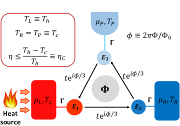
Figure 1: (Color online) Schematic of a triple-quantum-dot thermoelectric heat engine with a magnetic flux $\Phi$. Three quantum dots (energy levels are denoted as $E_{i}$, $i=L,R,P$) are connected to three electrodes. The electrochemical potentials and temperatures of the electrodes labeled in the figure. The tunneling rate between the dots and the electrodes is denoted by $\Gamma$. We consider the situation when both the $R$ and $P$ electrodes are in contact with a cold heat bath with temperature $T_{c}$, while the $L$ electrode is connected to a hot heat bath with temperature $T_{h}$.

As shown in Fig. 1, we consider a nanoscale thermoelectric device consisting of three quantum dots (QDs) coupled to three electrodes. This is a minimal model to demonstrate the set-up with two output electric currents. Although this model has been studied before Saito et al. (2011); Balachandran et al. (2013); Brandner and Seifert (2013); Stark et al. (2014), the configuration with two output electric currents has never been studied in the time-reversal symmetry broken regime. This model is valid when the Coulomb interaction in the QDs can be neglected Buttiker (1988). Each QD is coupled to the nearby reservoir and we thus employ the indices $1/2/3$ to label the leads $L/R/P$, respectively Jiang et al. (2015).

Hoppings between QDs are affected by the magnetic flux $\Phi$ piercing through the device at the center with the phase $\phi/3$ assigned to each of the hoppings ($\phi=2\pi\Phi/\Phi_{0}$ where $\Phi_{0}$ is flux quantum). The system is described by the Hamiltonian Saito et al. (2011)

$$\hat{H}=\hat{H}_{qd}+\hat{H}_{lead}+\hat{H}_{tun},$$ (10)

where

$$\hat{H}_{qd}=\sum_{i=1,2,3}E_{i}d_{i}^{\dagger}d_{i}+(te^{i\phi/3}d_{i+1}^{\dagger}d_{i}+{\rm H.c.}),$$ (11)

$$\hat{H}_{lead}=\sum_{i=1,2,3}\sum_{k}\varepsilon_{k}c^{\dagger}_{ik}c_{ik},$$ (12)

$$\hat{H}_{tun}=\sum_{i,k}V_{ik}d^{\dagger}_{i}c_{ik}+{\rm H.c.}.$$ (13)

Here, $d_{i}^{{\dagger}}$ and $d_{i}$ create and annihilate an electron in the $i$th QD with an energy $E_{i}$, respectively, $t$ is the tunneling amplitude between the QDs. $c_{ik}^{{\dagger}}$ and $c_{ik}$ create and annihilate an electron in the $i$-th electrode with the energy $E_{i}$ ($i=1,2,3$).

The chemical potential and temperature of three reservoirs are denoted by $\mu_{i}$ and $T_{i}$ ($i=L,R,P$), respectively. For each reservoir, there are an electric and a heat currents flowing out of the reservoir. In total there are six currents. However, only four of them are independent, due to charge and energy conservation Saito et al. (2011). We choose the charge and heat currents flowing out of the $L$ and $P$ reservoirs as the independent currents which are denoted as $I_{e}^{i}$ and $I_{Q}^{i}$ ($i=L,P$), respectively. The corresponding thermodynamic forces are

$$F_{e}^{i}=\frac{\mu_{i}-\mu_{R}}{e},\quad F_{Q}^{i}=\frac{T_{i}-T_{R}}{T_{i}}\quad(i=L,P).$$ (14)

where $e<0$ is the electronic charge. We focus on the set-up where $L$ reservoir is connected to the hot bath and the $R$ and $P$ reservoirs are connected to the cold bath, i.e., $T_{L}=T_{h}$ and $T_{P}=T_{R}=T_{c}$. There are two independent output electric currents, $I_{e}^{L}$ and $I_{e}^{P}$ (i.e., the charge currents flowing out of the $L$ and $P$ reservoirs), whereas there is only one input heat current $I_{Q}\equiv I_{Q}^{L}$ (i.e., the heat current flowing out of the hot reservoir $L$) with the corresponding force $F_{Q}\equiv F_{Q}^{L}$.

With such a set-up, the phenomenological Onsager transport equation is written in the linear-response regime as

$$\begin{pmatrix}\vec{I}_{e}\\ {I}_{Q}\\ \end{pmatrix}=\begin{pmatrix}\hat{\mathcal{M}}_{ee}&\hat{\mathcal{M}}_{eQ}\\ \hat{\mathcal{M}}_{Qe}&{\mathcal{M}}_{QQ}\\ \end{pmatrix}\begin{pmatrix}\vec{F}_{e}\\ {F}_{Q}\\ \end{pmatrix},$$ (15)

where the symbols $e$ and $Q$ are used to abbreviate the indices of forces and currents for charge and heat, respectively (i.e., $\vec{I}_{e}=(I_{e}^{L},I_{e}^{P})^{T}$, $\vec{F}_{e}=(F_{e}^{L},F_{e}^{P})^{T}$, $I_{Q}\equiv I_{Q}^{L}$, and $F_{Q}\equiv F_{Q}^{L}$; here the superscript $T$ stands for vector/matrix transpose). $\hat{\mathcal{M}}_{ee}$ denotes the $2\times 2$ charge conductivity tensor, the $2\times 1$ matrix $\hat{\mathcal{M}}_{eQ}$ describes the Seebeck effect, while the matrix $\hat{\mathcal{M}}_{Qe}$ describes the Peltier effect. The $1\times 1$ matrix (scalar) ${\mathcal{M}}_{QQ}$ represents the heat conductivity. For systems with time-reversal symmetry (e.g., $\phi=0,\pi$), Onsager’s reciprocal relation gives $\hat{\mathcal{M}}_{eQ}=\hat{\mathcal{M}}_{Qe}^{T}$. In contrast, for time-reversal broken systems, they are not equal to each other.

The output power and energy efficiency of the thermoelectric heat engine are written respectively as

$$W=-\vec{I}_{e}^{T}\vec{F}_{e}=-(\vec{F}_{e}^{T}\hat{\mathcal{M}}_{ee}\vec{F}_{e}+\vec{F}_{e}^{T}\hat{\mathcal{M}}_{eQ}{F}_{Q})>0,$$ (16)

and

$$\eta=\frac{W}{{I}_{Q}}=-\frac{\vec{F}_{e}^{T}\hat{\mathcal{M}}_{ee}\vec{F}_{e}+\vec{F}_{e}^{T}\hat{\mathcal{M}}_{eQ}{F}_{Q}}{\hat{\mathcal{M}}_{Qe}\vec{F}_{e}+{\mathcal{M}}_{QQ}{F}_{Q}}\leq\eta_{C}.$$ (17)

Here $\eta_{C}=1-T_{c}/T_{h}={\mathcal{F}}_{Q}$ is the Carnot efficiency which is the absolute upper bound for the attainable energy efficiency due to the second-law of thermodynamics of thermodynamics.

III Maximal efficiency and power for time-reversal broken systems

We note that in the linear-response regime the energy efficiency is invariant under the scaling transformation $\vec{F}_{e}\to a\vec{F}_{e}$ and $F_{Q}\to aF_{Q}$ with $a$ being an arbitrary constant. In comparison, the output power scales as $W\to a^{2}W$. We can then fix $F_{Q}$ and obtain the maximal energy efficiency by solving the following differential equation,

$$\frac{\partial\eta}{\partial\vec{F}_{e}}=0.$$ (18)

We obtain that

$$\vec{F}_{e}=-\frac{1}{2}\left[\eta_{\max}\left(\overline{\hat{\mathcal{M}}_{ee}}\right)^{-1}\hat{\mathcal{M}}^{T}_{Qe}{F}_{Q}+\left(\overline{\hat{\mathcal{M}}_{ee}}\right)^{-1}\hat{\mathcal{M}}_{eQ}{F}_{Q}\right].$$ (19)

Here we define

$$\overline{\hat{\mathcal{M}}_{ee}}\equiv\frac{1}{2}(\hat{\mathcal{M}}_{ee}+\hat{\mathcal{M}}^{T}_{ee})$$ (20)

as the symmetric charge conductivity tensor. Inserting Eq. (19) into Eq. (17), we arrive at

$$\eta_{\max}=\eta_{C}\frac{\lambda_{1}-\lambda_{2}(\eta_{\max}/\eta_{C})^{2}}{4-2(\lambda_{2}(\eta_{\max}/\eta_{C})+\lambda_{3})}.$$ (21)

Solving the above quadratic equation, we obtain the maximal efficiency as

$$\eta_{\max}=\eta_{C}\frac{2-\lambda_{3}-\sqrt{(2-\lambda_{3})^{2}-\lambda_{1}\lambda_{2}}}{\lambda_{2}}.~{}$$ (22)

Here,

$$\lambda_{1}\equiv\hat{\mathcal{M}}^{T}_{eQ}\left(\overline{\hat{\mathcal{M}}_{ee}}\right)^{-1}\hat{\mathcal{M}}_{eQ}{\mathcal{M}}^{-1}_{QQ},$$ (23a)

$$\lambda_{2}\equiv\hat{\mathcal{M}}_{Qe}\left(\overline{\hat{\mathcal{M}}_{ee}}\right)^{-1}\hat{\mathcal{M}}^{T}_{Qe}{\mathcal{M}}^{-1}_{QQ},$$ (23b)

$$\lambda_{3}\equiv\hat{\mathcal{M}}_{Qe}\left(\overline{\hat{\mathcal{M}}_{ee}}\right)^{-1}\hat{\mathcal{M}}_{eQ}{\mathcal{M}}^{-1}_{QQ}.$$ (23c)

are three dimensionless parameters that characterize the thermoelectric transport properties of the system. The output power at maximum efficiency is

$$W(\eta_{\max})=W_{0}\left[\lambda_{1}-\lambda_{2}\left(\frac{\eta_{\max}}{\eta_{C}}\right)^{2}\right],\quad W_{0}\equiv\frac{1}{4}{\mathcal{M}}_{QQ}{F}^{2}_{Q}.~{}$$ (24)

Similarly, we can obtain the maximal output power with fixed $F_{Q}$ by solving the following equation

$$\frac{\partial W}{\partial\vec{F}_{e}}=0,$$ (25)

which yields

$$W_{\max}=\lambda_{1}W_{0}.~{}$$ (26)

Meanwhile, the efficiency at maximum output power is Van den Broeck (2005); Golubeva and Imparato (2012)

$$\eta(W_{\max})=\eta_{C}\frac{\lambda_{1}}{4-2\lambda_{3}}.~{}$$ (27)

Comparing the energy efficiency and output power for the above two optimization schemes, we find that

$$\frac{\eta_{\max}}{\eta(W_{\max})}=1+\frac{\lambda_{2}}{\lambda_{1}}\left(\frac{\eta_{\max}}{\eta_{C}}\right)^{2},~{}$$ (28)

and

$$\frac{W(\eta_{\max})}{W_{\max}}=1-\frac{\lambda_{2}}{\lambda_{1}}\left(\frac{\eta_{\max}}{\eta_{C}}\right)^{2}.~{}$$ (29)

The above trade-off relations between the optimization of the efficiency and power is presented graphically in Fig. 2. These relations also reveal two important properties: First, the performance of the thermoelectric engine is better when $\lambda_{2}<\lambda_{1}$ compared with the situation with $\lambda_{2}>\lambda_{1}$. In addition, when $\lambda_{2}<\lambda_{1}$, the efficiency at maximal output power can possibly exceed the Curzon-Ahlborn limit Curzon and Ahlborn (1975) in the linear-response $\eta_{CA}=\eta_{C}/2$. Second, for $\lambda_{2}<\lambda_{1}$, the second-law of thermodynamics does not forbid the Carnot efficiency at finite output power. Although there have been many debates on such a possibility Benenti et al. (2011); Shiraishi et al. (2016b); Raz et al. (2016); Allahverdyan et al. (2013); Benenti et al. (2013); Holubec and Ryabov (2018), our study here opens a regime for further investigation of such an issue in quantum heat engines without the limitation of having only one electric and one heat currents.

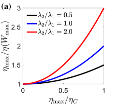
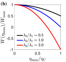
Figure 2: (Color online) Trade-off relations for optimal efficiency and power, Eqs. (28) and (29). (a) $\eta_{\max}/\eta(W_{\max})$ and (b) $W(\eta_{\max})/W_{\max}$ as functions of $\eta_{\max}/\eta_{C}$ for various $\lambda_{2}/\lambda_{1}$.

We now make two important remarks. First, the above results are valid for the situation with multiple output electric currents. This can be readily verified through the vectorial (matrix) formulation used in the above discussions. Second, the second-law of thermodynamics imposes the following constraints on the dimensionless parameters,

$$\lambda_{1}\geq 0,\quad\lambda_{2}\geq 0,\quad\lambda_{1}+\lambda_{2}+2\lambda_{3}\leq 4.~{}$$ (30)

The derivation of the above constraints goes as follows. The entropy production rate associated with the thermoelectric transport is Entin-Wohlman et al. (2014)

$$T_{R}\dot{\mathcal{S}} =\vec{I}_{e}^{T}\vec{F}_{e}+{I}_{Q}{F}_{Q}$$ (31)

$$=\begin{pmatrix}\vec{F}_{e}\,\,\,{F}_{Q}\end{pmatrix}\begin{pmatrix}\hat{\mathcal{M}}_{ee}&\hat{\mathcal{M}}_{eQ}\\ \hat{\mathcal{M}}_{Qe}&{\mathcal{M}}_{QQ}\\ \end{pmatrix}\begin{pmatrix}\vec{F}_{e}\\ {F}_{Q}\\ \end{pmatrix}$$

The second-law of thermodynamics requires $\dot{\mathcal{S}}\geq 0$ for all values of $\vec{F}_{e}$ and ${F}_{Q}$, which is equivalent to require the following matrix to be positive semi-definite,

$$\begin{pmatrix}\overline{\hat{\mathcal{M}}_{ee}}&\frac{\hat{\mathcal{M}}^{T}_{eQ}+\hat{\mathcal{M}}_{Qe}}{2}\\ \frac{\hat{\mathcal{M}}^{T}_{Qe}+\hat{\mathcal{M}}_{eQ}}{2}&{\mathcal{M}}_{QQ}\\ \end{pmatrix}.$$ (32)

Therefore, ${\mathcal{M}}_{QQ}\geq 0$ and the matrix $\overline{\hat{\mathcal{M}}_{ee}}$ is positive semi-definite. In addition, the determinant of the above matrix is positive semi-definite which yields

$$\left|\overline{\hat{\mathcal{M}}_{ee}}\right|\left|{\mathcal{M}}_{QQ}-\frac{\hat{\mathcal{M}}^{T}_{eQ}+\hat{\mathcal{M}}_{Qe}}{2}\left(\overline{\hat{\mathcal{M}}_{ee}}\right)^{-1}\frac{\hat{\mathcal{M}}^{T}_{Qe}+\hat{\mathcal{M}}_{eQ}}{2}\right|\geq 0,$$ (33)

where $|\,|$ is the determinant of the matrix. From these positive semi-definite properties, one can deduce Eq. (30) straightforwardly.

We now compare our results with previous studies on thermoelectric energy conversion in time-reversal broken mesoscopic systems. In all previous studies, the charge and heat currents flowing out of the $P$ terminal are tuned to vanish by adjusting the chemical potential and temperature at the $P$ terminal (often called as a probe-terminal in mesoscopic physics). Under such constraints, there are effectively only one heat current and one electric current in the system. Thermoelectric transport is then described by a $2\times 2$ Onsager matrix Saito et al. (2011); Balachandran et al. (2013); Brandner and Seifert (2013, 2015); Stark et al. (2014); Benenti et al. (2017). In this limit, the matrices $\hat{\mathcal{M}}_{ee}$, $\hat{\mathcal{M}}_{eQ}$ and $\hat{\mathcal{M}}_{Qe}$ become scalar quantities. From the definition in Eq. (23), one finds that for such a set-up

$$\lambda_{3}^{2}=\lambda_{1}\lambda_{2}.~{}$$ (34)

The above constraint is the main limitation of previous studies, which is overcome in this work. As a consequence, the maximum efficiency in our set-up can exceed that in previous set-ups, as shown in Fig. 3(a). In the figure, the black dot represent the limit (34) considered in previous studies. It is seen that the maximum efficiency can be improved by going beyond such a limit when $\lambda_{1}<\lambda_{2}$. Because of the power-efficiency trade-off, the higher efficiency is achieved at lower output power, as shown in Fig. 3(b). Figs. 3(c) and 3(d) show the maximal efficiency and the output power at such an efficiency. It is seen that large efficiency and power can be simultaneous obtained when $\lambda_{1}>\lambda_{2}$.

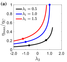
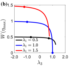
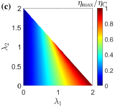
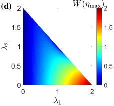
Figure 3: (Color online) (a) $\eta_{\max}/\eta_{C}$ and (b) $W(\eta_{\max})$ as functions of $\lambda_{3}$ for different $\lambda_{1}$, where $\lambda_{2}=1$. The black dots represent the limit given by Eq. (34). (c) $\eta_{\max}$ and (d) $\eta(W_{\max})$ as functions of $\lambda_{1}$ and $\lambda_{2}$ for $\lambda_{3}=1$. The white region is forbidden by the second-law of thermodynamics. The unit of the output power is $W_{0}$.

IV Upper bounds for efficiency and power

The bounds for the maximal efficiency $\eta_{max}$ and efficiency at the maximum power $\eta(W_{max})$ are reached at the reversible limit with $\lambda_{1}+\lambda_{2}+2\lambda_{3}=4$, leading to

$$\eta_{\max}|_{\rm{bound}}=\left\{\begin{aligned} &\eta_{C}\frac{\lambda_{1}}{\lambda_{2}},\quad\rm{if}\quad\lambda_{1}<\lambda_{2},\\ &\eta_{C},\quad\quad\,\rm{if}\quad\lambda_{1}\geq\lambda_{2}.\end{aligned}\right.~{}$$ (35)

The above results are presented graphically in Fig. 4(a) for various $\lambda_{1}$ and $\lambda_{2}$. The upper bound for the efficiency at the maximum output power is

$$\eta(W_{\max})|_{\rm{bound}}=\eta_{C}\frac{\lambda_{1}}{\lambda_{1}+\lambda_{2}}.~{}$$ (36)

From the above, the Curzon-Ahlborn limit Curzon and Ahlborn (1975); Seifert (2012) for the energy efficiency at maximum power $\eta=\eta_{C}/2$ can in principle be overcome for $\lambda_{1}>\lambda_{2}$. A particularly interesting regime is when $\lambda_{1}\gg\lambda_{2}$ where both the maximal efficiency and the efficiency at maximum power are bounded by the Carnot efficiency.

Combining Eq. (35) and Eq. (36), we find the ratio between those bounds for energy efficiency,

$$\frac{\eta_{\max}}{\eta(W_{\max})}|_{\rm{bound}}=\left\{\begin{aligned} &1+\frac{\lambda_{1}}{\lambda_{2}},\quad\rm{if}\quad\lambda_{1}<\lambda_{2},\\ &1+\frac{\lambda_{2}}{\lambda_{1}},\quad\rm{if}\quad\lambda_{1}\geq\lambda_{2}.\end{aligned}\right.$$ (37)

Meanwhile, the ratio between those bounds for output power is given by

$$\frac{W(\eta_{\max})}{W_{\max}}|_{\rm{bound}}=\left\{\begin{aligned} &1-\frac{\lambda_{1}}{\lambda_{2}},\quad\rm{if}\quad\lambda_{1}<\lambda_{2},\\ &1-\frac{\lambda_{2}}{\lambda_{1}},\quad\rm{if}\quad\lambda_{1}\geq\lambda_{2}.\end{aligned}\right.$$ (38)

As presented graphically in Figs. 4(c) and 4(d) for various $\lambda_{1}$ and $\lambda_{2}$, the trade-off between the optimal efficiency and power is significantly reduced when $\lambda_{1}\gg\lambda_{2}$, which implies that in this regime, large energy efficiency and power can be obtained simultaneously.

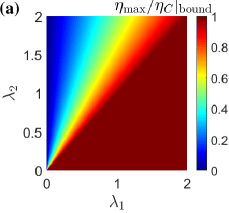
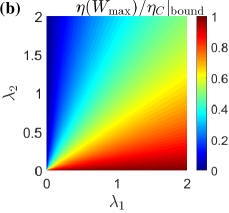
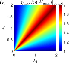
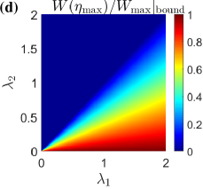
Figure 4: (Color online) Bounds on efficiency and power. (a) $\eta_{\max}|_{\rm{bound}}$, (b) $\eta(W_{\max})|_{\rm{bound}}$, (c) $\eta_{\max}/\eta(W_{\max})|_{\rm{bound}}$ and (d) $W(\eta_{\max})/W_{\max}|_{\rm{bound}}$ as functions of $\lambda_{1}$ and $\lambda_{2}$.

V Linear-response coefficients in a noninteracting QD system

We now investigate the optimal efficiency and power with a concrete model. The model adopted here is the three QDs model illustrated in Fig. 1, which has been studied extensively for the situations with only one electric and one heat currents. By releasing such a constraint, the charge and heat transport are described by the following equation,

$$\begin{pmatrix}I^{L}_{e}\\ I^{P}_{e}\\ I_{Q}\\ \end{pmatrix}=\begin{pmatrix}M_{11}&M_{12}&M_{13}\\ M_{21}&M_{22}&M_{23}\\ M_{31}&M_{32}&M_{33}\\ \end{pmatrix}\begin{pmatrix}F^{L}_{e}\\ F^{P}_{e}\\ F_{Q}\\ \end{pmatrix},$$ (39)

The coherent flow of charge and heat through a noninteracting QD system can be described using the Landauer-Bütiker theory. The charge and heat currents flowing out of the left reservoir are given by Sivan and Imry (1986); Butcher (1990)

$$I^{L}_{e} =\frac{2e}{h}\int dE\sum_{i}[({\mathcal{T}}_{iL}(E)f_{L}(E)-{\mathcal{T}}_{Li}(E)f_{R}(E))],$$ (40a)

$$I_{Q} =\frac{2}{h}\int dE\sum_{i}(E-\mu_{L})[{\mathcal{T}}_{iL}(E)f_{L}(E)-{\mathcal{T}}_{Li}(E)f_{R}(E)],$$ (40b)

where $f_{i}(E)=\{\exp[(E-\mu_{i})/k_{B}T_{i}]+1\}^{-1}$ is the Fermi function and ${\mathcal{T}}_{ij}$ is the transmission probability from terminal $j$ to terminal $i$, $h$ is the Planck constant. The factor of two comes from the spin degeneracy of electrons. Analogous expression can be written for $I^{P}_{e}$, provided the label $L$ is substituted by $P$ in (40a).

The Onsager coefficients $M_{ij}$ are obtained from the linear expansion of the electronic currents $I_{e}^{i}$ ($i=L,P$) and the heat current $I_{Q}$ in terms of the thermodynamic forces Sivan and Imry (1986); Butcher (1990),

$$M_{11} =\frac{2e^{2}}{hk_{B}T}\int_{-\infty}^{\infty}dE\sum_{i\neq L}{\mathcal{T}}_{Li}(E)F(E),$$ (41)

$$M_{12} =-\frac{2e^{2}}{hk_{B}T}\int_{-\infty}^{\infty}dE{\mathcal{T}}_{LP}(E)F(E),$$

$$M_{13} =M_{31}=\frac{2e}{hk_{B}T}\int_{-\infty}^{\infty}dE(E-\mu)\sum_{i\neq L}{\mathcal{T}}_{Li}(E)F(E),$$

$$M_{21} =-\frac{2e^{2}}{hk_{B}T}\int_{-\infty}^{\infty}dE{\mathcal{T}}_{PL}(E)F(E),$$

$$M_{22} =\frac{2e^{2}}{hk_{B}T}\int_{-\infty}^{\infty}dE\sum_{i\neq P}{\mathcal{T}}_{Pi}(E)F(E),$$

$$M_{23} =-\frac{2e}{hk_{B}T}\int_{-\infty}^{\infty}dE(E-\mu){\mathcal{T}}_{PL}(E)F(E),$$

$$M_{32} =-\frac{2e}{hk_{B}T}\int_{-\infty}^{\infty}dE(E-\mu){\mathcal{T}}_{LP}(E)F(E),$$

$$M_{33} =\frac{2}{hk_{B}T}\int_{-\infty}^{\infty}dE(E-\mu)^{2}\sum_{i\neq L}{\mathcal{T}}_{Li}(E)F(E).$$

where $F(E)\equiv\{4\cosh^{2}[(E-\mu)/k_{B}T]\}^{-1}$.

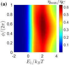
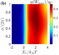
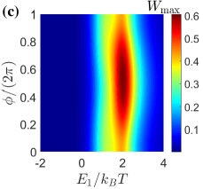
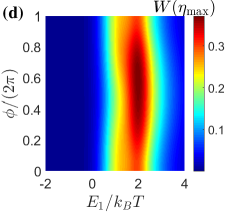
Figure 5: (Color online) Optimal efficiency and power in a triple-QD thermoelectric engine. (a) $\eta_{\max}$, (b) $\eta(W_{\max})$, (c) $W_{\max}$, and (d) $W(\eta_{\max})$ as the functions of $E_{1}$ and $\phi$. The other parameters are $t=-0.2k_{B}T$, $\Gamma=0.5k_{B}T$, $\mu=0$, $E_{2}=1.0k_{B}T$ and $E_{3}=2.0k_{B}T$.

The transmission probability ${\mathcal{T}}_{ij}(E)$ is calculated as  Balachandran et al. (2013)

$${\mathcal{T}}_{ij}={\rm Tr}[\Gamma_{i}(E)G(E)\Gamma_{j}(E)G^{\dagger}(E)],$$ (42)

where the (retarded) Green’s function for the QD system is $G(E)\equiv(E-H_{qd}-i\Gamma/2)^{-1}$, the damping rate $\Gamma=2\pi\sum_{k}|V_{ik}|^{2}\delta(\omega-\varepsilon_{ik})$ is assumed to be a constant for all three leads.

When an external magnetic field $\Phi$ is applied to the system, the laws of physics remain unchanged if time $t$ is replaced by $-t$, provided that simultaneously the magnetic field ${\Phi}$ is replaced by $-{\Phi}$. In this case, the transport coefficients meet the Onsager-Casimir relations Datta (1995)

$$M_{ij}({\phi})=M_{ji}(-{\phi}).$$ (43)

It is seen from Fig. 5 that the optimal efficiency and power vary strongly with the QD energy $E_{1}$ and the magnetic flux $\phi$. For these cases, the dependence on the QD energy is stronger than that on the magnetic flux. The efficiency and power are large when $E_{1}\approx 2k_{B}T$. The maximum efficiency $\eta_{\max}$ can reach $0.6\eta_{C}$. The results here reveal that a small external magnetic field can improve both the power and efficiency, when starting from the time-reversal limit of $\phi=\pi$.

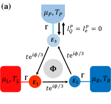
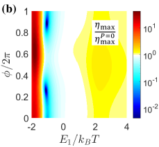
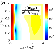
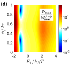
Figure 6: (Color online) (a) Schematic of the triple-QD thermoelectric engine when the electric current $I_{e}^{P}$ and heat current $I_{Q}^{P}$ vanish (denoted as $P=0$ briefly). (b)-(d) Comparing the optimal efficiency and power for the $P=0$ limit and the case with two output electric currents for various QD energy $E_{1}$ and magnetic flux $\phi$: (b) the maximal efficiency, (c) the efficiency at maximum power, and (d) the maximum output power. The other parameters are $t=-0.2k_{B}T$, $\mu=0$, $E_{2}=1.0k_{B}T$ and $E_{3}=2.0k_{B}T$.

In Fig. 6, we compare explicitly the performance of our three-terminal quantum heat engine with the previously studied limit. The latter is illustrated in Fig. 6(a), where the heat and electric currents flowing out of the $P$ terminal vanish by adjusting the chemical potential $\mu_{P}$ and temperature $T_{P}$. In this limit (denoted as $P=0$ briefly) there are only one electric and one heat currents, yielding the relation in Eq. (34). As shown in Figs. 6(b), Fig. 6(c) and Fig. 6(d), the maximal efficiency, the efficiency at maximum power, and the maximum output power can be significantly improved by releasing the limit of $P=0$. Our quantum heat engine with two output electric currents demonstrate superior efficiency and power for a large range of parameters.

VI Conclusion

In conclusion, we derived the optimal efficiency and power, and their trade-off relations for a three-terminal thermoelectric engine with two output electric currents. These results go beyond previous studies with time-reversal symmetry Jiang (2014a), and the time-reversal broken systems Benenti et al. (2011); Brandner et al. (2013) with only one electric current, revealing universalities in multi-terminal thermoelectric energy conversion differing from the existing theories. Numerical calculations for a triple-QD thermoelectric engine show that the efficiency and power can be substantially improved for the set-ups with two output electric currents compared with previous set-ups with only one electric current. We also find regimes where the energy efficiency and output power can be optimized at close conditions. Our results offer useful guidelines for the search of high-performance thermoelectric systems in the mesoscopic regime, with particular emphasizes on multi-terminal set-ups with multiple output electric currents.

References

- Butcher (1990) PN Butcher, “Thermal and electrical transport formalism for electronic microstructures with many terminals,” J. Phys.: Condens. Matter 2, 4869 (1990).
- Dubi and Di Ventra (2011) Y. Dubi and Massimiliano Di Ventra, “Colloquium: Heat flow and thermoelectricity in atomic and molecular junctions,” Rev. Mod. Phys. 83, 131–155 (2011).
- Li et al. (2012) Nianbei Li, Jie Ren, Lei Wang, Gang Zhang, Peter Hänggi, and Baowen Li, “Colloquium: Phononics: Manipulating heat flow with electronic analogs and beyond,” Rev. Mod. Phys. 84, 1045–1066 (2012).
- Sothmann et al. (2015) Björn Sothmann, Rafael Sánchez, and Andrew N Jordan, “Thermoelectric energy harvesting with quantum dots,” Nanotechnology 26, 032001 (2015).
- Jiang and Imry (2016) Jian-Hua Jiang and Yoseph Imry, “Linear and nonlinear mesoscopic thermoelectric transport with coupling with heat baths,” C. R. Phys. 17, 1047 – 1059 (2016).
- Benenti et al. (2017) Giuliano Benenti, Giulio Casati, Keiji Saito, and Robert S. Whitney, “Fundamental aspects of steady-state conversion of heat to work at the nanoscale,” Phys. Rep. 694, 1 – 124 (2017).
- Entin-Wohlman et al. (2014) O. Entin-Wohlman, J.-H. Jiang, and Y. Imry, “Efficiency and dissipation in a two-terminal thermoelectric junction, emphasizing small dissipation,” Phys. Rev. E 89, 012123 (2014).
- Jiang (2014a) Jian-Hua Jiang, “Thermodynamic bounds and general properties of optimal efficiency and power in linear responses,” Phys. Rev. E 90, 042126 (2014a).
- Bauer et al. (2016) Michael Bauer, Kay Brandner, and Udo Seifert, “Optimal performance of periodically driven, stochastic heat engines under limited control,” Phys. Rev. E 93, 042112 (2016).
- Proesmans et al. (2016a) Karel Proesmans, Bart Cleuren, and Christian Van den Broeck, “Power-efficiency-dissipation relations in linear thermodynamics,” Phys. Rev. Lett. 116, 220601 (2016a).
- Pietzonka and Seifert (2018) Patrick Pietzonka and Udo Seifert, “Universal trade-off between power, efficiency, and constancy in steady-state heat engines,” Phys. Rev. Lett. 120, 190602 (2018).
- Whitney (2014) Robert S. Whitney, “Most efficient quantum thermoelectric at finite power output,” Phys. Rev. Lett. 112, 130601 (2014).
- Whitney (2015) Robert S. Whitney, “Finding the quantum thermoelectric with maximal efficiency and minimal entropy production at given power output,” Phys. Rev. B 91, 115425 (2015).
- Verley et al. (2014) Gatien Verley, Massimiliano Esposito, Tim Willaert, and Christian Van den Broeck, “The unlikely carnot efficiency,” Nat. Commun. 5, 4721 (2014).
- Polettini et al. (2015) M. Polettini, G. Verley, and M. Esposito, “Efficiency statistics at all times: Carnot limit at finite power,” Phys. Rev. Lett. 114, 050601 (2015).
- Jiang et al. (2015) Jian-Hua Jiang, Bijay Kumar Agarwalla, and Dvira Segal, “Efficiency statistics and bounds for systems with broken time-reversal symmetry,” Phys. Rev. Lett. 115, 040601 (2015).
- Proesmans et al. (2016b) Karel Proesmans, Yannik Dreher, Mom čilo Gavrilov, John Bechhoefer, and Christian Van den Broeck, “Brownian duet: A novel tale of thermodynamic efficiency,” Phys. Rev. X 6, 041010 (2016b).
- Sánchez and Serra (2011) D. Sánchez and L. Serra, “Thermoelectric transport of mesoscopic conductors coupled to voltage and thermal probes,” Phys. Rev. B 84, 201307 (2011).
- Sánchez and Büttiker (2011) Rafael Sánchez and Markus Büttiker, “Optimal energy quanta to current conversion,” Phys. Rev. B 83, 085428 (2011).
- Jiang et al. (2012) Jian-Hua Jiang, Ora Entin-Wohlman, and Yoseph Imry, “Thermoelectric three-terminal hopping transport through one-dimensional nanosystems,” Phys. Rev. B 85, 075412 (2012).
- Sothmann et al. (2012) Björn Sothmann, Rafael Sánchez, Andrew N. Jordan, and Markus Büttiker, “Rectification of thermal fluctuations in a chaotic cavity heat engine,” Phys. Rev. B 85, 205301 (2012).
- Jiang et al. (2013a) Jian-Hua Jiang, Ora Entin-Wohlman, and Yoseph Imry, “Hopping thermoelectric transport in finite systems: Boundary effects,” Phys. Rev. B 87, 205420 (2013a).
- Simine and Segal (2013) Lena Simine and Dvira Segal, “Path-integral simulations with fermionic and bosonic reservoirs: Transport and dissipation in molecular electronic junctions,” J. Chem. Phys. 138, 214111 (2013).
- Sothmann et al. (2013) Björn Sothmann, Rafael Sánchez, Andrew N Jordan, and Markus Büttiker, “Powerful energy harvester based on resonant-tunneling quantum wells,” New J. Phys. 15, 095021 (2013).
- Jiang et al. (2013b) Jian-Hua Jiang, Ora Entin-Wohlman, and Yoseph Imry, “Three-terminal semiconductor junction thermoelectric devices: improving performance,” New J. Phys. 15, 075021 (2013b).
- Mazza et al. (2015) Francesco Mazza, Stefano Valentini, Riccardo Bosisio, Giuliano Benenti, Vittorio Giovannetti, Rosario Fazio, and Fabio Taddei, “Separation of heat and charge currents for boosted thermoelectric conversion,” Phys. Rev. B 91, 245435 (2015).
- Brandner and Seifert (2013) Kay Brandner and Udo Seifert, “Multi-terminal thermoelectric transport in a magnetic field: bounds on onsager coefficients and efficiency,” New J. Phys. 15, 105003 (2013).
- Agarwalla et al. (2015) Bijay Kumar Agarwalla, Jian-Hua Jiang, and Dvira Segal, “Full counting statistics of vibrationally assisted electronic conduction: Transport and fluctuations of thermoelectric efficiency,” Phys. Rev. B 92, 245418 (2015).
- Li and Jiang (2016) Lijie Li and Jian-Hua Jiang, “Staircase quantum dots configuration in nanowires for optimized thermoelectric power,” Sci. Rep. 6, 31974 (2016).
- Yamamoto et al. (2016) Kaoru Yamamoto, Ora Entin-Wohlman, Amnon Aharony, and Naomichi Hatano, “Efficiency bounds on thermoelectric transport in magnetic fields: The role of inelastic processes,” Phys. Rev. B 94, 121402 (2016).
- Agarwalla et al. (2017) Bijay Kumar Agarwalla, Jian-Hua Jiang, and Dvira Segal, “Quantum efficiency bound for continuous heat engines coupled to noncanonical reservoirs,” Phys. Rev. B 96, 104304 (2017).
- Macieszczak et al. (2018) Katarzyna Macieszczak, Kay Brandner, and Juan P. Garrahan, “Unified thermodynamic uncertainty relations in linear response,” Phys. Rev. Lett. 121, 130601 (2018).
- Jiang and Imry (2018) Jian-Hua Jiang and Yoseph Imry, “Near-field three-terminal thermoelectric heat engine,” Phys. Rev. B 97, 125422 (2018).
- Shiraishi et al. (2016a) Naoto Shiraishi, Keiji Saito, and Hal Tasaki, “Universal trade-off relation between power and efficiency for heat engines,” Phys. Rev. Lett. 117, 190601 (2016a).
- Lu et al. (2019) Jincheng Lu, Rongqian Wang, Jie Ren, Manas Kulkarni, and Jian-Hua Jiang, “Quantum-dot circuit-qed thermoelectric diodes and transistors,” Phys. Rev. B 99, 035129 (2019).
- Petersson et al. (2012) K. D. Petersson, L. W. McFaul, M. D. Schroer, M. Jung, J. M. Taylor, A. A. Houck, and J. R. Petta, “Circuit quantum electrodynamics with a spin qubit,” Nature 490, 380 (2012).
- Hwang et al. (2013) Sun-Yong Hwang, David Sánchez, Minchul Lee, and Rosa López, “Magnetic-field asymmetry of nonlinear thermoelectric and heat transport,” New J. Phys. 15, 105012 (2013).
- Matthews et al. (2014) J. Matthews, F. Battista, D. Sánchez, P. Samuelsson, and H. Linke, “Experimental verification of reciprocity relations in quantum thermoelectric transport,” Phys. Rev. B 90, 165428 (2014).
- Thierschmann et al. (2015) H. Thierschmann, R. Sánchez, B. Sothmann, F. Arnold, C. Heyn, W. Hansen, H. Buhmann, and L. W. Molenkamp, “Three-terminal energy harvester with coupled quantum dots,” Nat. Nanotech. 10, 854 (2015).
- Roche et al. (2015) B. Roche, P. Roulleau, T. Jullien, Y. Jompol, I. Farrer, D. A. Ritchie, and D. C. Glattli, “Harvesting dissipated energy with a mesoscopic ratchet,” Nat. comm. 6, 6738 (2015).
- Cui et al. (2018) Longji Cui, Ruijiao Miao, Kun Wang, Dakotah Thompson, Linda Angela Zotti, Juan Carlos Cuevas, Edgar Meyhofer, and Pramod Reddy, “Peltier cooling in molecular junctions,” Nat. Nanotech. 13, 122 (2018).
- Humphrey et al. (2002) T. E. Humphrey, R. Newbury, R. P. Taylor, and H. Linke, “Reversible quantum brownian heat engines for electrons,” Phys. Rev. Lett. 89, 116801 (2002).
- Humphrey and Linke (2005) T. E. Humphrey and H. Linke, “Reversible thermoelectric nanomaterials,” Phys. Rev. Lett. 94, 096601 (2005).
- Iyyappan and Ponmurugan (2018) I. Iyyappan and M. Ponmurugan, “General relations between the power, efficiency, and dissipation for the irreversible heat engines in the nonlinear response regime,” Phys. Rev. E 97, 012141 (2018).
- Jiang (2014b) Jian-Hua Jiang, “Enhancing efficiency and power of quantum-dots resonant tunneling thermoelectrics in three-terminal geometry by cooperative effects,” J. Appl. Phys. 116, 194303 (2014b).
- Lu et al. (2017) Jincheng Lu, Rongqian Wang, Yefeng Liu, and Jian-Hua Jiang, “Thermoelectric cooperative effect in three-terminal elastic transport through a quantum dot,” J. Appl. Phys. 122, 044301 (2017).
- Jiang and Imry (2017) Jian-Hua Jiang and Yoseph Imry, “Enhancing thermoelectric performance using nonlinear transport effects,” Phys. Rev. Applied 7, 064001 (2017).
- Benenti et al. (2011) Giuliano Benenti, Keiji Saito, and Giulio Casati, “Thermodynamic bounds on efficiency for systems with broken time-reversal symmetry,” Phys. Rev. Lett. 106, 230602 (2011).
- Brandner et al. (2013) Kay Brandner, Keiji Saito, and Udo Seifert, “Strong bounds on onsager coefficients and efficiency for three-terminal thermoelectric transport in a magnetic field,” Phys. Rev. Lett. 110, 070603 (2013).
- Saito et al. (2011) Keiji Saito, Giuliano Benenti, Giulio Casati, and Toma ž Prosen, “Thermopower with broken time-reversal symmetry,” Phys. Rev. B 84, 201306 (2011).
- Balachandran et al. (2013) Vinitha Balachandran, Giuliano Benenti, and Giulio Casati, “Efficiency of three-terminal thermoelectric transport under broken time-reversal symmetry,” Phys. Rev. B 87, 165419 (2013).
- Brandner and Seifert (2015) Kay Brandner and Udo Seifert, “Bound on thermoelectric power in a magnetic field within linear response,” Phys. Rev. E 91, 012121 (2015).
- Stark et al. (2014) Julian Stark, Kay Brandner, Keiji Saito, and Udo Seifert, “Classical nernst engine,” Phys. Rev. Lett. 112, 140601 (2014).
- Curzon and Ahlborn (1975) F. L. Curzon and B. Ahlborn, “Efficiency of a carnot engine at maximum power output,” Am. J. Phys. 43, 22–24 (1975).
- Buttiker (1988) M. Buttiker, “Coherent and sequential tunneling in series barriers,” IBM J. Res. Dev. 32, 63–75 (1988).
- Van den Broeck (2005) C. Van den Broeck, “Thermodynamic efficiency at maximum power,” Phys. Rev. Lett. 95, 190602 (2005).
- Golubeva and Imparato (2012) N. Golubeva and A. Imparato, “Efficiency at maximum power of interacting molecular machines,” Phys. Rev. Lett. 109, 190602 (2012).
- Shiraishi et al. (2016b) Naoto Shiraishi, Keiji Saito, and Hal Tasaki, “Universal trade-off relation between power and efficiency for heat engines,” Phys. Rev. Lett. 117, 190601 (2016b).
- Raz et al. (2016) O. Raz, Y. Subaş ı, and R. Pugatch, “Geometric heat engines featuring power that grows with efficiency,” Phys. Rev. Lett. 116, 160601 (2016).
- Allahverdyan et al. (2013) Armen E. Allahverdyan, Karen V. Hovhannisyan, Alexey V. Melkikh, and Sasun G. Gevorkian, “Carnot cycle at finite power: Attainability of maximal efficiency,” Phys. Rev. Lett. 111, 050601 (2013).
- Benenti et al. (2013) Giuliano Benenti, Giulio Casati, and Jiao Wang, “Conservation laws and thermodynamic efficiencies,” Phys. Rev. Lett. 110, 070604 (2013).
- Holubec and Ryabov (2018) Viktor Holubec and Artem Ryabov, “Cycling tames power fluctuations near optimum efficiency,” Phys. Rev. Lett. 121, 120601 (2018).
- Seifert (2012) Udo Seifert, “Stochastic thermodynamics, fluctuation theorems and molecular machines,” Rep. Prog. Phys. 75, 126001 (2012).
- Sivan and Imry (1986) U. Sivan and Y. Imry, “Multichannel landauer formula for thermoelectric transport with application to thermopower near the mobility edge,” Phys. Rev. B 33, 551–558 (1986).
- Datta (1995) Supriyo Datta, Electronic transport in mesoscopic systems (Cambridge university press, Cambridge, UK, 1995).