Electric circuit simulations of $n$th-Chern insulators in $2n$-dimensional space
and their non-Hermitian generalizations for arbitral $n$

Abstract

We show that topological phases of the Dirac system in arbitral even dimensional space are simulated by $LC$ electric circuits with operational amplifiers. The lattice Hamiltonian for the hypercubic lattice in $2n$ dimensional space is characterized by the $n$-th Chern number. The boundary state is described by the Weyl theory in $2n-1$ dimensional space. They are well observed by measuring the admittance spectrum. They are different from the disentangled $n$-th Chern insulators previously reported, where the $n$-th Chern number is a product of the first Chern numbers. The results are extended to non-Hermitian systems with complex Dirac masses. The non-Hermitian $n$-th Chern number remains to be quantized for the complex Dirac mass.

I Introduction

Topological insulators were originally discovered in condensed matter physics. Now the notion has been extended to cold atomsGold , photonicsTopoPhoto2014 ; TopoPhoto and acousticsTopoAco ; Xue ; Alex ; WZhu . A recent finding is that it is also applicable to electric circuitsComPhys ; TECNature . Various topological phases have been simulated by electric circuitsComPhys ; TECNature ; Garcia ; Hel ; Lu ; EzawaTEC ; Hofmann ; EzawaLCR ; EzawaChern ; EzawaMajo . In this context, non-Hermitian topological systems are among hottest topics of artificial topological systemsZeu ; Konotop ; Mark ; Scho ; Pan ; Hoda ; NoriSOTI ; EzawaLCR . Nevertheless, all these phases are also realizable in condensed matter in principle. It is an interesting problem to explore exotic topological phases which would never exist in condensed matter.

An obvious example is the topological phase in the spatial $d$ dimensions ($d$Ds) with $d\geq 4$. The four-dimensional (4D) quantum Hall effect is one of them4D . It is simulated via 2D quasi-crystalsKraus or topological pumpings in photonic systemsZil ; Ozawa and optical latticesPrice ; Lohse . They are characterized by the second-Chern number. In the same way, the 6D quantum Hall effect is realized in 3D topological pumpings6D . However, these phases are disentangled, where they are decomposed into two or three independent copies of 2D quantum Hall insulators. Accordingly, the second- or third-Chern numbers become products of the first-Chern numbers. We seek genuine higher-dimensional topological phases, which cannot be decomposed into lower-dimensional topological phases.

In this paper, we show that topological phases of the Dirac system in any even dimensional space are simulated by $LC$ electric circuits with operational amplifiers. Especially, we construct topological phases characterized by the $n$-th Chern number in $2n$Ds for arbitral $n$. We start with the Dirac Hamiltonian in higher dimensions. Then, we analyze lattice models defined on the hypercubic lattice. The $n$-th Chern number is analytically calculated since it is determined by the Dirac theory at the $2^{2n}$ high-symmetry points. Then we show that the boundary states are described by the Weyl theory in (2n-1)D. They are manifested by calculating the density of states (DOS), which is proportional to $|E|^{2n-2}$. Finally, we point out that they are well signaled by admittance spectrum.

II Model Hamiltonian

The Dirac Hamiltonian in $2n$D space is given by

$$H_{2n}=\int d^{2n}k\left[\psi^{\dagger}\left(x\right)\Gamma_{j}\left(-i\partial_{j}\right)\psi\left(x\right)+M\psi^{\dagger}\Gamma_{0}\psi\right],$$ (1)

where $\Gamma_{\mu}$ with $j=1,2,\cdots,2n$ and $\mu=0,1,2,\cdots,2n$ are the gamma matrices satisfying the Clifford algebra $\left\{\Gamma_{\mu},\Gamma_{\nu}\right\}=2\delta_{\mu\nu}I$, while $M$ is the Dirac mass. The system becomes non-Hermitian when the mass $M$ is taken to be complex. All the analysis is valid both for Hermitian and non-Hermitian systems.

The gamma matrix $\Gamma_{\mu}^{2n}$ in $2n$Ds has a $2^{n}$ dimensional representation, which is recursively defined by

$$\Gamma_{0}^{2n} = \sigma_{x}\otimes\mathbb{I}^{2n-2},\quad\Gamma_{2n}^{2n}=\sigma_{z}\otimes\mathbb{I}^{2n-2},$$

$$\Gamma_{j}^{2n} = \sigma_{y}\otimes\Gamma_{j}^{2n-2},\text{ }$$ (2)

for $1\leq j\leq 2n-1$, and $\Gamma_{0}^{2}=\sigma_{z}$, $\Gamma_{1}^{2}=\sigma_{x}$, $\Gamma_{2}^{2}=\sigma_{y}$.

The corresponding lattice model isGolt ; TQFT ,

$$H_{2n}\left(k\right)=\sum_{\mu=0}^{2n}\psi^{\dagger}\left(k\right)d^{\mu}\Gamma_{\mu}\psi\left(k\right),$$ (3)

where

$$d^{0}=m+t\sum_{j=1}^{2n}\cos k_{j},\qquad d^{j}=\lambda\sin k_{j},$$ (4)

with the on-site potential $m$, the hopping amplitude $t$ and the spin-orbital interaction $\lambda$. The energy spectrum is given by $E=\pm\sqrt{\sum_{\mu=0}^{2n}\left(d^{\mu}\right)^{2}}$.

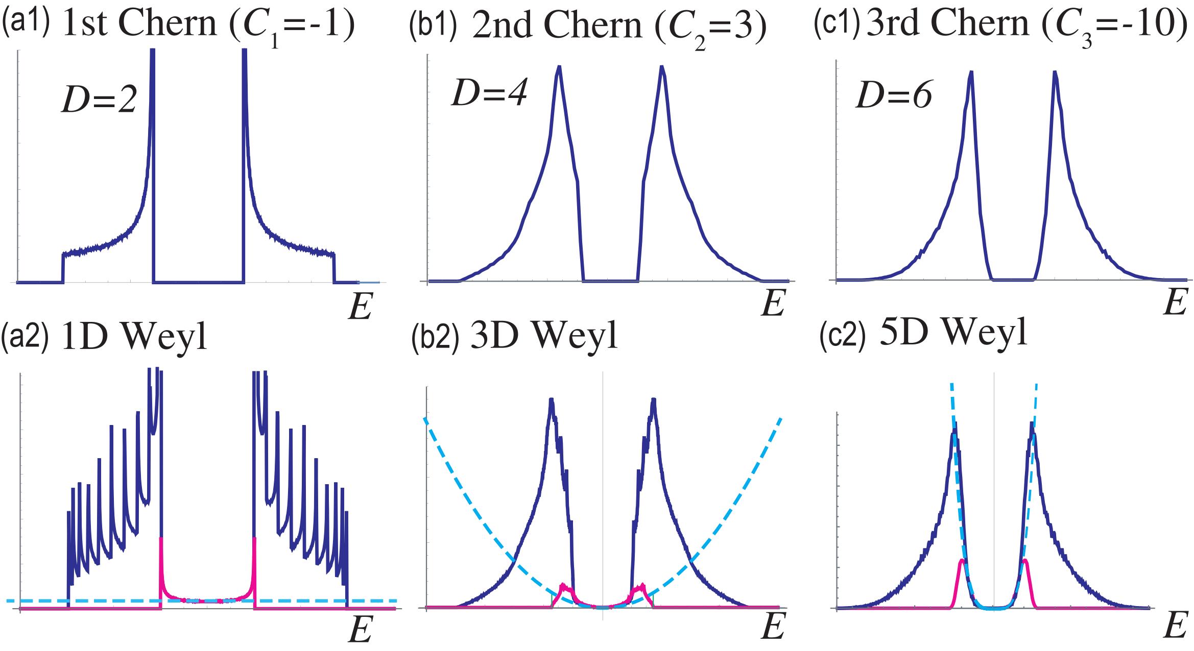
Figure 1: (a1)–(c1) DOS of the bulk in $n$-th Chern insulators for the Hermitian system as a function of the energy $E$ for (a) $D=2$ with $C_{1}=-1$, (b) $D=4$ with $C_{2}=3$, and (c) $D=6$ with $C_{3}=-10$. There are finite gaps, dictating that the systems are insulators. (a2)–(c2) DOS of the boundary states as a function of the energy $E$. The dark blue curves represent the DOS for all bands numerically obtained, the magenta curves represent the DOS for the energy (19) analytically obtained, and the dotted cyan curves represent the DOS for the energy (20) analytically obtained. These numerical results are well fitted by analytical results of the Weyl theory in the vicinity of the Fermi energy. We have set $t=\lambda=m=1$.

First, we show the bulk DOS of the Hermitian system in Fig.1(a1)-(c1). The system is an insulator due to a finite gap, which indicates that the system is an insulator.

Next, we show the energy spectrum in the Re$E$-Im$E$ planeFu for the non-Hermitian system in Fig.2(a1)-(c1). The system remains to be an insulator. The two bulk spectra are separated by a line given by Re$E=0$. This structure is called a line gapKawabataST , which is a generalization of an insulator to the non-Hermitian system.

The gap closes at the $2^{2n}$ high-symmetry points $\boldsymbol{K}=\left(K_{1},K_{2},\cdots,K_{2n}\right)$, where $K_{j}=0,\pi$. By evaluating (4) at these points, we obtain a set of $2^{2n}$ Dirac Hamiltonians (3) together with

$$d^{0}\left(\boldsymbol{K}\right) = m+t\sum_{j=1}^{2n}\left(-1\right)^{K_{j}/\pi}\equiv\bar{m},$$ (5)

$$d^{j}\left(\boldsymbol{K}\right) = \left(-1\right)^{K_{j}/\pi}\lambda k_{j},$$ (6)

where $d^{0}\left(\boldsymbol{K}\right)$ is the Dirac mass at the point $\boldsymbol{K}$. We define the sign of the Dirac Hamiltonian by $\eta\left(\boldsymbol{K}\right)\equiv\left(-1\right)^{\sum K_{j}/\pi}=\pm 1$.

III Non-Hermitian $n$-th Chern number

In the classification table, the topological insulator without any symmetry is classified by the $\mathbb{Z}$ index for both of the HermitianSchny ; Ryu and non-Hermitian systemsKawabataST . In the case of the Hermitian system, the topological number is the $n$-th Chern number. It is also applicable to the non-Hermitian system by using the following definition.

As a generalization of the non-Hermitian "first" Chern numberKohmoto ; Fu ; Yao2 ; Kunst ; KawabataChern ; Philip ; Chen ; EzawaChern , we define the non-Hermitian $n$-th Chern number as

$$C_{n}=\frac{1}{\left(2\pi\right)^{n}}\int\frac{1}{n!}\bigwedge\limits^{n}Fd^{2n}k,$$ (7)

where $F$ is the non-Hermitian non-Abelian Berry curvature,

$$F_{ij}^{\alpha\beta}=\partial_{i}A_{j}^{\alpha\beta}-\partial_{j}A_{i}^{\alpha\beta}+i\left[A_{i},A_{j}\right]^{\alpha\beta},$$ (8)

with the non-Hermitian Berry connectionKohmoto ; Zhu ; Yin ; Lieu

$$A_{i}^{\alpha\beta}\left(k\right)=-i\left\langle\psi_{\alpha}^{\text{L}}\left(k\right)\right|\partial_{k_{i}}\left|\psi_{\beta}^{\text{R}}\left(k\right)\right\rangle.$$ (9)

Here, $\left|\psi_{\beta}^{\text{R}}\left(k\right)\right\rangle$ is the right-eigen states $H\left|\psi_{\beta}^{\text{R}}\left(k\right)\right\rangle=E\left|\psi_{\beta}^{\text{R}}\left(k\right)\right\rangle$, and $\left|\psi_{\beta}^{\text{L}}\left(k\right)\right\rangle$ is the right-eigen states $H^{\dagger}\left|\psi_{\beta}^{\text{L}}\left(k\right)\right\rangle=E^{\ast}\left|\psi_{\beta}^{\text{L}}\left(k\right)\right\rangle$.

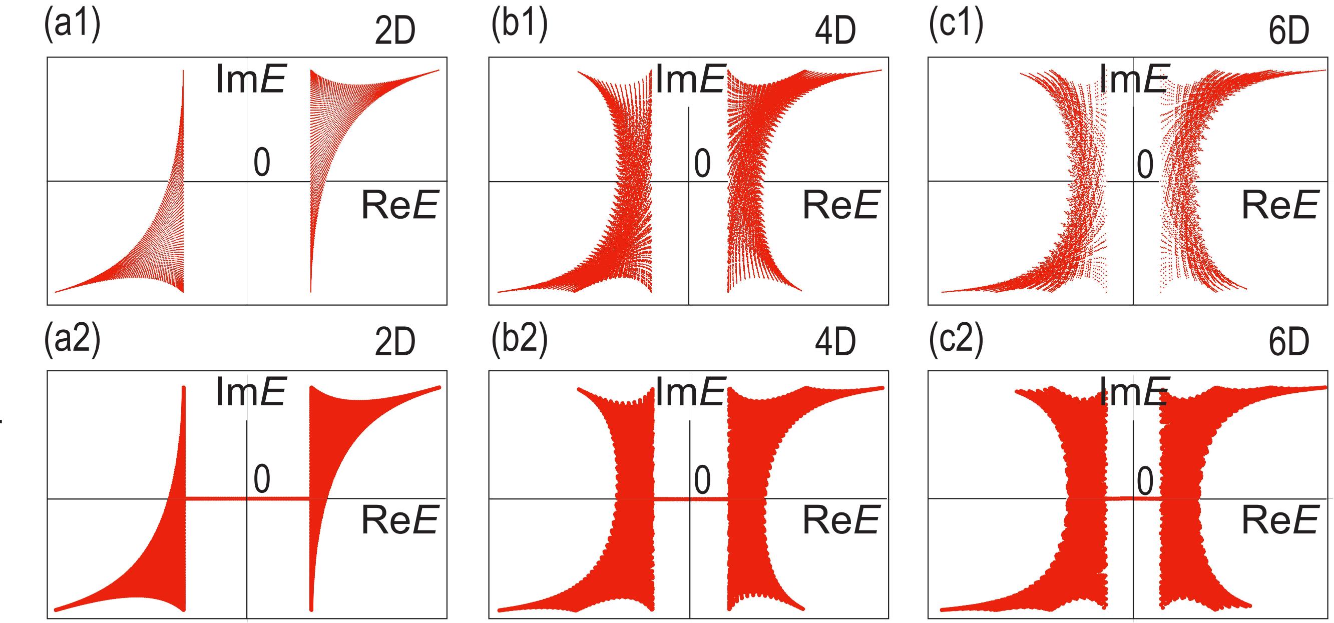
Figure 2: Energy spectrum in the Re$E$-Im$E$ plane for (a) $D=2$ ($L=100$), (b) $D=4$ ($L=25$) and (c) $D=6$ ($L=25$), where $L$ is the length of the hypercube. (a1)–(c1) There are gaps in the bulk spectrum, showing that the system is an insulator. (a2)–(2) There are boundary states connecting two bulk spectra, which is on the Im$E=0$ line. They are Weyl boundary states. We have set $t=\lambda=1$ and $m=1+0.1i$.

Substituting (5) and (6) into (7), the $n$-th Chern number is given by

$$C_{n}\left(K_{\mu}\right)=\eta\frac{\left(4n-1\right)!!}{2^{n-1}\left(2n-1\right)!}\int d^{2n}k\frac{\bar{m}}{\left(k^{2}+\bar{m}^{2}\right)^{\left(2n+1\right)/2}},$$ (10)

which is explicitly calculated as

$$C_{n}\left(K_{\mu}\right)=\eta\frac{\bar{m}}{2\sqrt{\bar{m}^{2}}}.$$ (11)

It reads $C_{n}\left(K_{\mu}\right)=\eta/2$ for Re$\left[\bar{m}\right]>0$ and $C_{n}\left(K_{\mu}\right)=-\eta/2$ for Re$\left[\bar{m}\right]<0$. It is quantized even for a complex mass.

The topological phase boundaries are determined by the massless condition $\bar{m}\left(K_{\mu}\right)=0$, which is independent of the value of the spin-orbital interaction $\lambda$.

Then the total $n$-th Chern number for the lattice Hamiltonian is

$$C_{n}=\sum_{K_{j}}C_{n}\left(K_{j}\right),$$ (12)

where the summation is taken over all the highest symmetry points. We show the $n$-th Chern number as a function of $m/t$ in Fig.3. It is always quantized and jumps when the mass becomes zero.

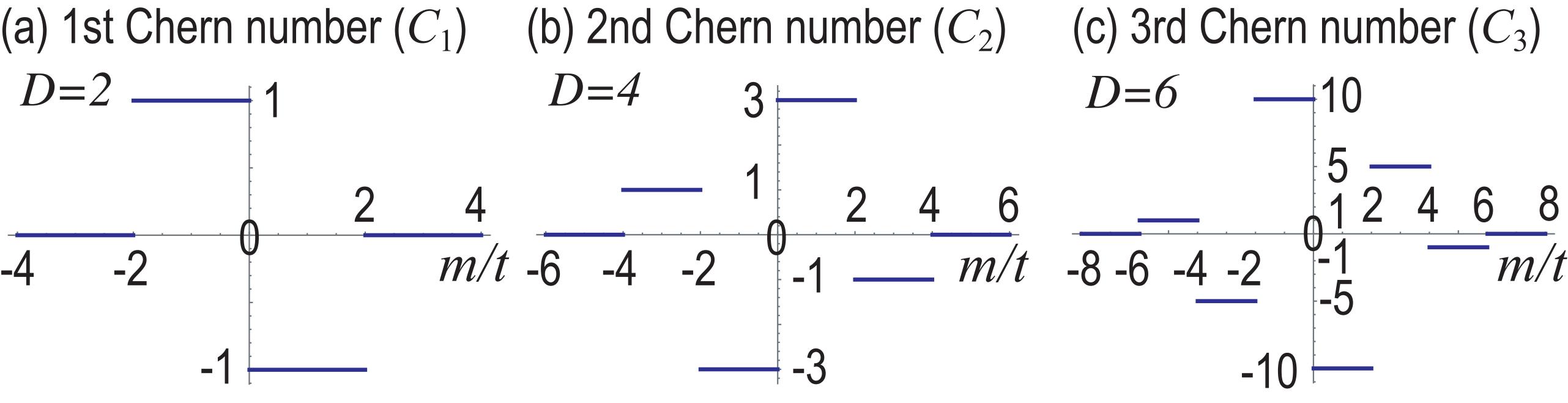
Figure 3: $n$-th Chern number as a function of $m$ for (a) $D=2$, (b) $D=4$ and (c) $D=6$. We have set $\lambda=1$.

IV Weyl Boundary states

The boundary states emerge in a topological phase of an insulator. Let us review the case of 2Ds, where we analyze a nanoribbon with a finite width along the $x_{2}$ axis. First of all, the dynamical degree of freedom with respect to $x_{2}$ is frozen by the Jackiw-Rebbi solution of the Dirac equationJR , where the mass has a spatial dependence. On the other hand, the lattice structure along the $x_{1}$ axis allows us to introduce the crystal momentum $k_{1}$. Consequently, the dynamical degree of freedom is carried solely by the momentum $k_{1}$ along the edge.

Similarly in 2$n$Ds, we analyze a nanostructure with a finite thickness along the $x_{2n}$ axis, while the other directions are periodic. We numerically calculate the energy spectrum of the non-Hermitian system in the Re$E$-Im$E$ plane as in Fig.2(a2)–(c2). There are lines connecting two separated bulk spectra along the Im$E=0$ line in topological phases. They are Weyl boundary states, which remains to be real even for the non-Hermitian system. It results in the emergence of a zero-energy solution, which is the Jackiw-Rebbi solution as we now demonstrate.

The Dirac equation describing the boundary states is given by

$$(\bar{m}\left(x_{2n}\right)\sigma_{x}\otimes\mathbb{I}^{2n-2} -i\lambda\partial_{x_{2n}}\sigma_{y}\otimes\mathbb{I}^{2n-2}$$

$$+\sum_{j=1}^{2n-1}k_{j}\sigma_{z}\otimes\Gamma_{j-1})\psi= 0,$$ (13)

where $\bar{m}\left(x_{2n}\right)$ is a spatially dependent mass,

$$\bar{m}\left(x_{2n}\right)=m_{0}\tanh\frac{x_{2n}}{\xi},$$ (14)

with $\xi$ the penetration depth. We seek a zero-energy solution by solving

$$\left(\begin{array}[]{cc}0&\bar{m}\left(x_{2n}\right)-\lambda\partial_{x_{2n}}\\ \bar{m}\left(x_{2n}\right)+\lambda\partial_{x_{2n}}&0\end{array}\right)\left(\begin{array}[]{c}\psi_{A}\\ \psi_{B}\end{array}\right)=0.$$ (15)

It is exactly given by the Jackiw-Rebbi solution,

$$\psi_{A} \propto \exp\left[-\frac{1}{\lambda}\int\bar{m}\left(x_{2n}\right)dx_{2n}\right],$$ (16)

$$\psi_{B} \propto \exp\left[\frac{1}{\lambda}\int\bar{m}\left(x_{2n}\right)dx_{2n}\right].$$ (17)

The zero-energy solutions exist when the integrands converge. We have shown that the Jackiw-Rebbi solution follows even in the non-Hermitian system.

Since the dynamical degree of freedom with respect to $x_{2n}$ is frozen, the dimensional reduction occurs from $2n$Ds to ($2n-1$)Ds, where the dynamical degrees of freedom are crystal momenta $k_{j}$ with $1\leq j\leq 2n-1$. The zero-energy solution is localized at the boundary, where the mass becomes zero. Hence, the boundary Hamiltonian is described by the Weyl Hamiltonian in ($2n-1$)Ds,

$$H_{2n-1}\left(k\right)=\sum_{j=1}^{2n-1}\psi^{\dagger}\left(k\right)d^{j}\Gamma_{j}\psi\left(k\right),$$ (18)

whose energy spectrum is given by

$$E\left(k\right)=\pm\left|\lambda\right|\sqrt{\sum_{j=1}^{2n-1}\sin^{2}k_{j}}.$$ (19)

In the vicinity of the Fermi level, the energy dispersion is linear,

$$E\left(k\right)=\pm\left|\lambda k\right|.$$ (20)

We show the boundary states numerically obtained as a function of $k_{x}$ and $k_{y}$ for the $n$-th Chern insulator based on the tight-binding Hamiltonian (3) in Fig.4, where we have set $k_{j}=0$ for $3\leq j\leq 2n-1$. It is well fitted by (19).

The DOS is defined by

$$\rho\left(E\right)=\int\delta\left(E-\lambda\sqrt{\sum_{j=1}^{2n-1}\sin^{2}k_{j}}\right)d^{2n-1}k,$$ (21)

which is proportional to

$$\rho\left(E\right)\propto\lambda\left|E\right|^{2n-2}$$ (22)

in the vicinity of the Fermi level.

We numerically calculate the DOS of the thin film in the case of the Hermitian system in Fig.1(a2)-(c2). In the vicinity of the Fermi level, the DOS of the total band is well fitted by the DOS determined by the boundary lattice Hamiltonian (19) and the DOS (22) of the Weyl Hamiltonian. The DOS of the Hamiltonian is observable by measuring admittance, as we shall see later. Thus, it is an experimental signature to detect higher-dimensional Weyl boundary states.

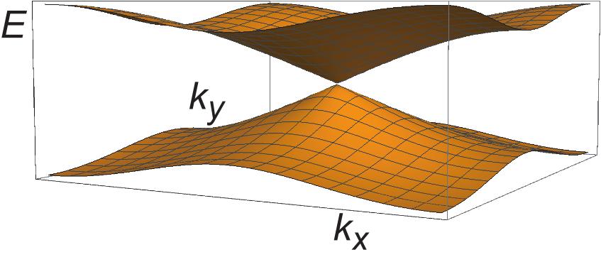
Figure 4: Cone structure of the Weyl boundary state. The vertical axis is $E$, while the horizontal axes are $k_{x}$ and $k_{y}$. We have set the other momenta are zero, $k_{j}=0$ for $3\leq j\leq 2n-1$. It does not depend on the dimension. The parameters are the same as Fig.2.

V Disentangled $n$-th Chern insulators

We comment on a trivial construction of the $n$-th Chern insulators, which are mainly studied in previous literatureKraus ; Zil ; Ozawa ; Price ; Lohse . We construct a Hamiltonian by a direct product of the first-Chern insulator in 2Ds as

$$H_{2n}\left(k\right)=\bigotimes\limits^{n}H_{2}\left(k\right).$$ (23)

Then the $n$-th Chern number is decomposed into

$$C_{n}=\left(\frac{1}{2\pi}\int d^{2}kF\right)^{n}=\prod\limits^{n}C_{1}.$$ (24)

It is also an $n$-th Chern insulator. However, it is disentangled and a trivial example since it is essentially a first-Chern insulator.

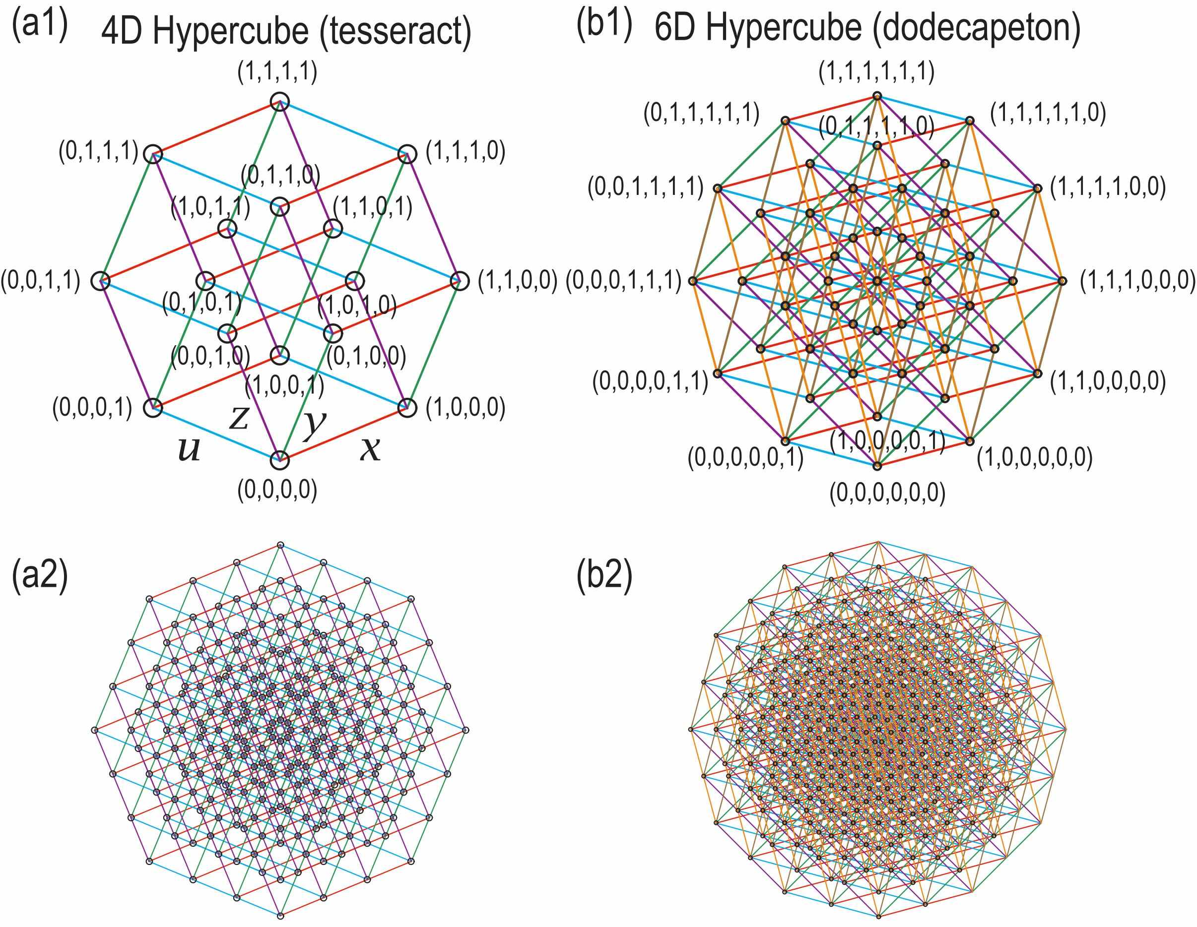
Figure 5: Projection of the hypercube onto the 2D plane. (a) 4D hypercube and (b) 6D hypercube. Circles represent the unit cell shown in Fig.6, and colored links represent the conection between two unit cells as in Fig.6. (a1) Electric circuit for the 4D hypercube with $L=1$. (a2) The one for the 4D hypercube with $L=3$. (b1) The one for the 6D hypercube with $L=1$. (b1) The one for the 6D hypercube with $L=2$. The coordinates are shown in (a1) and (b1).

VI Electric circuit realization

We next explain how to simulate the above model in higher dimensions by electric circuits. First, we note that a hypercubic lattice in any dimensions can be projected to a 2D plane as illustrated in Fig.5. The lattice points of a hypercube are projected to different positions in the 2D plane. Although the links cross each other, they can be avoided by using a bridge structure of wiring. We consider a hypercubic lattice structure in $2n$Ds whose unit cell contains $2^{2n}$ sites, which is the dimension of the $\Gamma$ matrix.

Let us explain an instance of the 4D lattice, i.e., the case of $n=2$. A single cube ($L=1$) contains $16$ sites as in Fig.5(a1). A pair of two sites are connected by a colored link, which is parallel to one of the four axes, i.e., the $x$-axis (red), the $y$-axis (green), the $z$-axis (purple) and the $u$-axis (cyan). A lattice with size $L=3$ is illustrated in Fig.5(a2), which is obtained by dividing an edge of a single cube into $L=3$ pieces.

Second, we associate one unit cell with each site, and one link circuit with each link: There are four types of link circuits in 4D lattice as illustrated in Fig.6. Actual forms of the unit cell and the link circuits are constructed by analyzing the Kirchhoff current law.

The Kirchhoff current law of the circuit under the application of an AC voltage $V\left(t\right)=V\left(0\right)e^{i\omega t}$ is given byComPhys ; TECNature ,

$$I_{a}\left(\omega\right)=\sum_{b}\mathcal{J}_{ab}\left(\omega\right)V_{b}\left(\omega\right),$$ (25)

where the sum is taken over all adjacent nodes $b$, and $\mathcal{J}_{ab}\left(\omega\right)$ is called the circuit Laplacian. The eigenvalues of the circuit Laplacian are called the admittance spectrum, which provides us with an information of the bulk spectrum of the corresponding Hamiltonian.

We explain the method to implement an electric circuit corresponding to the Hamiltonian. The Hamiltonian is written in the form of the $2n\times 2n$ matrix. Each component has the form of $e^{\pm ik_{\mu}}$, $-e^{\pm ik_{\mu}}$or $ie^{\pm ik_{\mu}}$. We express the term $e^{\pm ik_{\mu}}$ by capacitors $i\omega Ce^{\pm ik_{\mu}}$, the term $-e^{\pm ik_{\mu}}$ by inductors $-\frac{1}{i\omega L}e^{\pm ik_{\mu}}$, and the term $ie^{\pm ik_{\mu}}$ by operational amplifiers $iR_{X}e^{\pm ik_{\mu}}$ as in the case of the previous studiesComPhys ; TECNature ; Garcia ; Hel ; Lu ; EzawaTEC ; Hofmann ; EzawaChern ; EzawaMajo . We introduce operational amplifiers $R_{0}$ in order to make the Dirac mass complex. Then we connect each node by the capacitor $C_{0}$ and the inductor $L_{0}$ to the ground as in Fig.6(e).

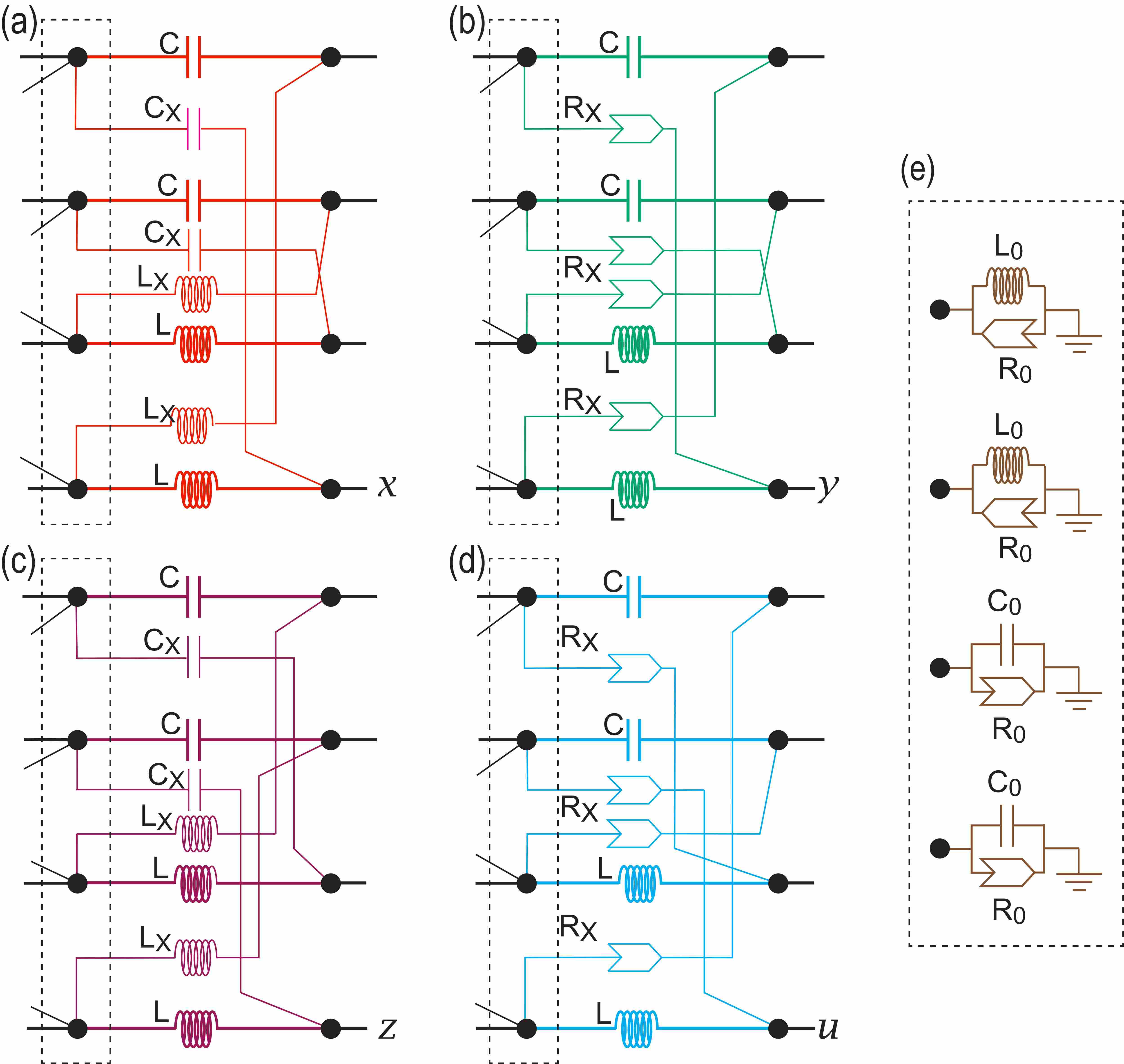
Figure 6: Basic elements for electric circuit realization of the second-Chern insulator on the 4D hypercubic lattice. The dotted rectangul represents the unit cell. Colored circuits in (a) red, (b) green, (c) purple and (d) cyan represent links parallel to four independent axes $x$, $y$, $z$ and $u$, respectively. (e) Each node in the unit cell is grounded either by a capacitance or an inductor with an operational amplifier. See also Fig.5 how to construct a whole circuit using the unit cell and links.

Let us explicitly show the implementation in the case of 4Ds. In order to make a circuit simple, we take a representation $\Gamma^{0}=\sigma_{z}\otimes I$, $\Gamma^{x}=\sigma_{x}\otimes\sigma_{x}$, $\Gamma^{y}=\sigma_{x}\otimes\sigma_{y}$, $\Gamma^{z}=\sigma_{x}\otimes\sigma_{z}$ and $\Gamma^{u}=\sigma_{y}\otimes I$ for the second-Chern insulator. We show the element of the circuit structure in Fig.6. We use these structures colored in red, green, purple and cyan as $x$, $y$, $z$ and $u$ links in Fig.5, while the unit cell is denoted by black dotted rectangles.

The circuit Laplacian is a sum of five terms in 4Ds, $\mathcal{J}=\sum_{\mu=0,x,y,z,u}\mathcal{J}_{\mu}$, with

$$\mathcal{J}_{0} = \left(\begin{array}[]{cccc}m^{+}&0&0&0\\ 0&m^{+}&0&0\\ 0&0&m^{-}&0\\ 0&0&0&m^{-}\end{array}\right),\quad$$ (30)

$$\mathcal{J}_{x} = \left(\begin{array}[]{cccc}f_{x}^{+}&0&0&g_{x}^{0}\\ 0&f_{x}^{+}&g_{x}^{0}&0\\ 0&g_{x}^{0}&f_{x}^{-}&0\\ g_{x}^{0}&0&0&f_{x}^{-}\end{array}\right),$$ (35)

$$\mathcal{J}_{y} = \left(\begin{array}[]{cccc}f_{y}^{+}&0&0&g_{y}^{-}\\ 0&f_{y}^{+}&g_{y}^{+}&0\\ 0&g_{y}^{-}&f_{y}^{-}&0\\ g_{y}^{+}&0&0&f_{y}^{-}\end{array}\right),$$ (40)

$$\mathcal{J}_{z} = \left(\begin{array}[]{cccc}f_{z}^{+}&0&g_{z}^{0}&0\\ 0&f_{z}^{+}&0&-g_{z}^{0}\\ g_{z}^{0}&0&f_{z}^{-}&0\\ 0&-g_{z}^{0}&0&f_{z}^{-}\end{array}\right),$$ (45)

$$\mathcal{J}_{u} = \left(\begin{array}[]{cccc}f_{u}^{+}&0&g_{u}^{-}&0\\ 0&f_{u}^{+}&0&g_{u}^{-}\\ g_{u}^{+}&0&f_{u}^{-}&0\\ 0&g_{u}^{+}&0&f_{u}^{-}\end{array}\right)$$ (50)

with

$$m^{+} =C_{0}-(i\omega R_{0})^{-1},$$ (51)

$$m^{-} =-(\omega^{2}L_{0})^{-1}+(i\omega R_{0})^{-1},$$ (52)

$$f_{j}^{+} =2C\cos k_{j}-2C,$$ (53)

$$f_{j}^{-} =-2(\omega^{2}L)^{-1}\cos k_{j}+2(\omega^{2}L)^{-1},$$ (54)

$$g_{j}^{+} =-(\omega^{2}L_{X})^{-1}e^{ik_{j}}+C_{X}e^{-ik_{j}},$$ (55)

$$g_{j}^{-} =C_{X}e^{ik_{j}}-(\omega^{2}L_{X})^{-1}e^{-ik_{j}},$$ (56)

$$g_{j}^{0} =(i\omega R_{X})^{-1}e^{ik_{j}}-(i\omega R_{X})^{-1}e^{-ik_{j}}.$$ (57)

The system becomes an $LC$ resonator.

Finally, we fix parameters in electric circuit so that the circuit Laplacian $\mathcal{J}$ is identical to the Hamiltonian $H$. It follows that $\mathcal{J}=i\omega H$, provided the resonance frequency is given by

$$\omega_{0}=1/\sqrt{LC}=1/\sqrt{L_{0}C_{0}},$$ (58)

and

$$t = C,\lambda=C_{X}=(\omega_{0}R_{X})^{-1},$$ (59)

$$m = -4nC+C_{0}-(i\omega R_{0})^{-1}.$$ (60)

An important observation is that we may change the mass $m$ by tuning $C_{0}$. Then, we may induce topological phase transitions by controlling the Chern number based on the formula (11) together with (5).

The eigenvalues of the circuit Laplacian give an admittance spectrumComPhys ; TECNature ; Garcia ; Hel ; Lu ; EzawaTEC . Then the DOS of the Laplacian is proportional to the DOS of the Hamiltonian. Thus, the DOS of the Laplacian is measured by the DOS of the admittance.

VII Discussions

We have shown that topological insulators in any dimensions are simulated by electric circuits. In elementary particle physics, the spatial dimension is believed to be higher than three according to string theory. On the other hand, the classification table of the topological insulator dictates the existence of the topological systems in higher dimensionsSchny ; Ryu ; KawabataST . However, these higher dimensional systems are impossible to approach experimentally. Our results will open a rout to study higher dimensional physics in laboratory.

The author is very much grateful to N. Nagaosa for helpful discussions on the subject. This work is supported by the Grants-in-Aid for Scientific Research from MEXT KAKENHI (Grants No. JP17K05490, No. JP15H05854 and No. JP18H03676). This work is also supported by CREST, JST (JPMJCR16F1 and JPMJCR1874).

References

- (1) N. Goldman, J. C. Budich, P. Zoller, Nat. Phys. 12, 639 (2016).
- (2) L. Lu, J. D. Joannopoulos and M. Soljačić, Nature Photonics 8, 821 (2014)
- (3) T. Ozawa, H. M. Price, A. Amo, N. Goldman, M. Hafezi, L. Lu, M. C. Rechtsman, D. Schuster, J. Simon, O. Zilberberg, and I. Carusotto Rev. Mod. Phys. 91, 015006 (2019)
- (4) Z. Yang, F. Gao, X. Shi, X. Lin, Z. Gao, Y. Chong, B. Zhang, Phys. Rev. Lett. 114, 114301 (2015)
- (5) H. Xue, Y. Yang, F. Gao, Y. Chong and B. Zhang, Nature Materials 18, 108 (2019).
- (6) X. Ni, M. Weiner, A. Alu, and A. B. Khanikaev, Nature Materials 18, 113 (2019).
- (7) W. Zhu, X. Fang, D. Li, Y. Sun, Y. Li, Y. Jing and H. Chen, Phys. Rev. Lett. 121, 124501 (2018)
- (8) C. H. Lee , S. Imhof, C. Berger, F. Bayer, J. Brehm, L. W. Molenkamp, T. Kiessling and R. Thomale, Communications Physics, 1, 39 (2018).
- (9) S. Imhof, C. Berger, F. Bayer, J. Brehm, L. Molenkamp, T. Kiessling, F. Schindler, C. H. Lee, M. Greiter, T. Neupert, R. Thomale, Nat. Phys. 14, 925 (2018).
- (10) M. Serra-Garcia, R. Susstrunk and S. D. Huber, Phys. Rev. B 99, 020304 (2019).
- (11) T. Helbig, T. Hofmann, C. H. Lee, R. Thomale, S. Imhof, L. W. Molenkamp and T. Kiessling, Phys. Rev. B 99, 161114 (2019).
- (12) Y. Lu, N. Jia, L. Su, C. Owens, G. Juzeliunas, D. I. Schuster and J. Simon, Phys. Rev. B 99, 020302 (2019).
- (13) M. Ezawa, Phys. Rev. B 98, 201402(R) (2018).
- (14) T. Hofmann, T. Helbig, C. H. Lee, M. Greiter, R. Thomale, arXiv:1809.08687.
- (15) M. Ezawa, Phys. Rev. B 99, 201411(R) (2019).
- (16) M. Ezawa, cond-arXiv:1904.03823
- (17) M. Ezawa, cond-arXiv:1902.03716
- (18) J. M. Zeuner, M. C. Rechtsman, Y. Plotnik, Y. Lumer, S. Nolte, M. S. Rudner, M. Segev, and A. Szameit, Phys. Rev. Lett. 115, 040402 (2015).
- (19) V. V. Konotop, J. Yang, and D. A. Zezyulin, Rev. Mod. Phys. 88, 035002 (2016).
- (20) K. G. Makris, R. El-Ganainy, D. N. Christodoulides, and Z. H. Musslimani, Phys. Rev. Lett. 100, 103904 (2008).
- (21) H. Schomerus, Opt. Lett. 38, 1912 (2013).
- (22) M. Pan, H. Zhao, P. Miao, S. Longhi, and L. Feng, Nat. Commun. 9, 1308 (2018).
- (23) H. Hodaei, A. U Hassan, S. Wittek, H. Garcia-Gracia, R. El-Ganainy, D. N. Christodoulides and M. Khajavikhan, Nature 548, 187 (2017).
- (24) T. Liu, Y.-R. Zhang, Q. Ai, Z. Gong, K. Kawabata, M. Ueda, F. Nori, Phys. Rev. Lett. 122, 076801 (2019)
- (25) S. C. Zhang and J. Hou, Science 294, 823 (2001)
- (26) Y. E. Kraus, Z. Ringel, and O. Zilberberg, Phys. Rev. Lett. 111, 226401 (2013)
- (27) O. Zilberberg, S. Huang, J. Guglielmon, M. Wang, K. P. Chen, Y. E. Kraus, and M. C. Rechtsman, Nature 553, 59 (2018).
- (28) T. Ozawa, H. M. Price, N. Goldman, O. Zilberberg, and I. Carusotto, Phys. Rev. A 93, 043827 (2016)
- (29) H. M. Price, O. Zilberberg, T. Ozawa, I. Carusotto, and N. Goldman, Phys. Rev. Lett. 115, 195303 (2015)
- (30) M. Lohse, C. Schweizer, H. M. Price, O. Zilberberg and I. Bloch, Nature 553, 55 (2018).
- (31) I. Petrides, H. M. Price, and O. Zilberberg, Phys. Rev. B 98, 125431 (2018)
- (32) M. F. L. Golterman, K. Jansen and D. B. Kaplan, Phys. Lett. B 301, 219 (1993)
- (33) X.-L. Qi, T. L. Hughes and S.-C. Zhang, Phys. Rev. B 78, 195424 (2008)
- (34) H. Shen, B. Zhen and L. Fu Phys. Rev. Lett. 120, 146402 (2018).
- (35) K. Kawabata, K. Shiozaki, M. Ueda, M. Sato, cond-mat/arXiv:1812.09133.
- (36) A. P. Schnyder, S. Ryu, A. Furusaki, A. W. W. Ludwig, Phys. Rev. B 78, 195125 (2008)
- (37) S. Ryu, A. P Schnyder, A. Furusaki and A. W. W. Ludwig, New J. Phys. 12 065010 (2010)
- (38) K. Esaki, M. Sato, K. Hasebe, and M. Kohmoto, Phys. Rev. B 84, 205128 (2011).
- (39) S. Yao, F. Song and Z. Wang, Phys. Rev. Lett. 121, 136802 (2018).
- (40) F. K. Kunst, E. Edvardsson, J. C. Budich and E. J. Bergholtz, Phys. Rev. Lett. 121, 026808 (2018).
- (41) K. Kawabata, K. Shiozaki and M. Ueda, Phys. Rev. B 98, 165148 (2018)
- (42) Timothy M. Philip, Mark R. Hirsbrunner, and Matthew J. Gilbert, Phys. Rev. B 98, 155430 (2018)
- (43) Y. Chen and H. Zhai, Phys. Rev. B 98, 245130 (2018).
- (44) B. Zhu, R. Lu and S. Chen, Phys. Rev. A 89, 062102 (2014).
- (45) C. Yin, H. Jiang, L. Li, Rong Lu and S. Chen, Phys. Rev. A 97, 052115 (2018).
- (46) S. Lieu, Phys. Rev. B 97, 045106 (2018).
- (47) R. Jackiw and C. Rebbi, Phys. Rev. D 13, 3398 (1976)