A unified construction for series representations and finite approximations of completely random measures

Abstract

Infinite-activity completely random measures (CRMs) have become important building blocks of complex Bayesian nonparametric models. They have been successfully used in various applications such as clustering, density estimation, latent feature models, survival analysis or network science. Popular infinite-activity CRMs include the (generalized) gamma process and the (stable) beta process. However, except in some specific cases, exact simulation or scalable inference with these models is challenging and finite-dimensional approximations are often considered. In this work, we propose a general and unified framework to derive both series representations and finite-dimensional approximations of CRMs. Our framework can be seen as an extension of constructions based on size-biased sampling of Poisson point process [46]. It includes as special cases several known series representations as well as novel ones. In particular, we show that one can get novel series representations for the generalized gamma process and the stable beta process. We also provide some analysis of the truncation error.

1 Introduction

Infinite-activity completely random measures (CRMs), and more generally functionals of infinite-activity Poisson random measures arise as building blocks of numerous modern structured statistical models. Examples include clustering and density estimation [49, 32, 33], spatial statistics [13, 56, 41], latent factor/trait models [24, 44, 59, 16, 3], network modeling [14, 60, 15, 17], recommendation systems [26], prediction, risk management and option pricing of financial assets [19] or survival analysis [28, 42]; see [40] for a review. Popular CRMs include the (generalized) gamma random measure (also known as tempered stable) [30, 13] or the (stable) beta random measure [28, 54]. Other popular random probability measures such as the Dirichlet process or the Pitman-Yor process are obtained by normalization or transformation of CRMs.
The use of statistical models based on infinite-activity CRMs poses a number of practical challenges regarding posterior inference and estimation. Except in some specific cases, most algorithms, either based on Gibbs sampling [31, 60], slice sampling [27, 23], mean-field variational inference [9, 21, 39] or sequential Monte Carlo [11],[4, Section 3.2.], require the use of a finite-dimensional approximation of the CRM. Finite-dimensional approximations can either be obtained by (i) truncating a series representation of the CRM, with stochastically decreasing weights, or (ii) by considering a finite measure with $n$ atoms and iid weights, converging in distribution to the CRM as $n$ tends to infinity. For example, for the beta process with scale parameter $\alpha>0$ and probability distribution $H$, the inverse Lévy series representation is [55]

$$G=\sum_{i=1}^{\infty}W_{i}\delta_{\theta_{i}},~{}~{}~{}\text{where}~{}~{}W_{i}=\prod_{j=1}^{i}\beta_{j},~{}~{}\beta_{i}\overset{\mathrm{i.i.d.}}{\sim}\operatorname{Beta}(\alpha,1),~{}~{}\theta_{i}\overset{\mathrm{i.i.d.}}{\sim}H,~{}~{}i=1,2\ldots,.$$ (1)

A classical finite-dimensional approximation with iid weights is [24]

$$\widetilde{G}_{n}=\sum_{i=1}^{n}\widetilde{W}_{n,i}\delta_{\widetilde{\theta}_{n,i}},~{}~{}~{}\text{where}~{}~{}\widetilde{W}_{n,i}\overset{\mathrm{i.i.d.}}{\sim}\operatorname{Beta}(\alpha/n,1),~{}~{}\widetilde{\theta}_{n,i}\overset{\mathrm{i.i.d.}}{\sim}H,~{}~{}i=1,\ldots,n.$$ (2)

Both representations are routinely used in Markov chain Monte Carlo and variational Bayes approximate inference algorithms [21, 45, 43]. Series and iid approximations are similarly used for the gamma process [60, 48] and the generalized gamma process [39]. Since the early work of [35] and [22] on the so-called inverse Lévy representation, various generic series representations of Poisson random measures have been proposed [12, 46, 50, 52]. Nested series representations have also been recently proposed for some specific CRMs [45, 43, 48]. Finite iid representations can be obtained using the infinite divisibility properties of the CRM [37] but as noted by [39], it generally does not lead to tractable representations, except in the gamma process case. Other ways of obtaining iid constructions are described in [29] for some family of CRMs. [18] provided a recent survey of the existing series representations and approximations as well as a truncation analysis.

The objective of this article is to present a general framework to obtain both series and iid representations of CRMs. Our construction builds on the definition of a Poisson random measure on an extended space; it generalizes the size-biased approach of [46], and admits as special cases both the size-biased and inverse-Lévy representations. We show that under this construction, one can draw connections between existing series and iid representations that appeared unrelated, and it allows to derive new series and iid representations. More precisely, we show how the iid representation of [39] is related to the size-biased construction of [46], derive novel series and iid representations of the generalized gamma and stable beta random measures. We also provide an asymptotic analysis of the truncation error for this class of approximations.
This article is organised as follows. In Section 2 we provide background material on completely random measures and some existing series representations for CRMs and describe the objectives. Section 3 describes the general construction for obtaining series and iid representations of CRMs. In Section 4 we describe a number of specific constructions, showing how one recovers some existing constructions as a particular case of our framework. In Section 5 we provide an analysis of the asymptotic truncation error, and discuss related approaches in Section 6. The proofs and additional background material are provided in the appendix.

Notations. For a measure $\nu$ on $S$ and a positive measurable function $h$ on $S$, write $\nu(h)=\int_{S}h(x)\nu(dx)$. Let $(\xi_{1},\xi_{2},\ldots,)$ be the ordered points of a unit-rate Poisson point process on $(0,\infty)$, that is $\xi_{1},\xi_{2}-\xi_{1},\xi_{3}-\xi_{2},\ldots$ are iid unit-rate exponential random variables. With a slight abuse of notation, we use the same notation for the distribution of a random variable and its pdf. For instance, the probability density function (pdf) of a gamma random variable $X\sim\operatorname{Gamma}(a,b)$ is written as $\operatorname{Gamma}(x;a,b)$.

2 Background

2.1 Completely random measures

Let $(S,\mathcal{S})$ be a measurable space where $S=(0,\infty)\times\Theta$. For any point $X=(W,\theta)\in S$, we refer to $W>0$ as the size of $X$. Let $N$ be a Poisson random measure on $S$ with mean measure $\nu(dw,d\theta)=\rho(dw)\mu_{w}(d\theta)$ where $\rho$ is a Borel measure on $(0,\infty)$, called size measure, satisfying

$$\int_{0}^{\infty}(1-e^{-w})\rho(dw)<\infty\text{ and }\int_{0}^{\infty}\rho(dw)=\infty$$ (3)

and $\mu_{w}(\cdot)$ is a Markov probability kernel from $(0,\infty)$ to $\Theta$. The linear functional

$$G=\int_{0}^{\infty}wN(dw,d\theta)$$

is an infinite-activity completely random measure [36] on $\Theta$ with random weights and random atoms. We write $G\sim\operatorname*{CRM}(\rho,\mu_{w})$. The conditions (3) imply that the atomic random measures $N$ and $W$ have an infinite number of atoms, and $W(\Theta)$ is almost surely finite. If $\mu_{w}=H$ does not depend on $w$, the CRM is said to be homogeneous. We assume in the rest of this article that one can easily simulate from $\mu_{w}$ (or $H$) and/or it admits a tractable density with respect to some reference measure (e.g. Lebesgue). Two popular examples of CRMs are the generalized gamma process (GGP) [30, 13], also known as (exponentially) tilted stable process, with size measure

$$\rho(dw)=\frac{\alpha}{\Gamma(1-\sigma)}w^{-1-\sigma}e^{-\tau w}dw$$ (4)

where $\alpha>0$, $\sigma\in(0,1)$ and $\tau\geq 0$, or $\sigma\leq 0$ and $\tau>0$, and the stable beta process (SBP) [28, 54] with

$$\rho(dw)=\frac{\alpha}{B(1-\sigma,c+\sigma)}w^{-\sigma-1}(1-w)^{c+\sigma-1}\mathds{1}_{\{0<w<1\}}dw,$$ (5)

where $\sigma\in(-\infty,1)$, $c>-\sigma$, $\alpha>0$ and $B(\cdot,\cdot)$ is the beta function. When $\sigma\geq 0$, both random measures are infinite-activity.

Remark 2.1.

The constructions described in this paper hold more generally when the first condition in Equation (3) is not satisfied, but $\int_{x}^{\infty}\rho(dw)<\infty$ for all $x$. Note that in this case $W(\Theta)=\infty$ almost surely. An example of this more general case is given in Section 4.4 where $\rho(dw)=w^{-2}dw$.

2.2 Objective

Our objective is to derive general series representations for the Poisson random measure $N$, or equivalently the CRM $G$, of the form

$$G=\sum_{i=1}^{\infty}W_{i}\delta_{\theta_{i}}$$ (6)

where the sizes $(W_{1},W_{2},\ldots)$, are stochastically ordered. That is, for any $w>0$, $\Pr(W_{i+1}>w)\leq\Pr(W_{i}>w).$ We write $W_{1}\succeq W_{2}\succeq\ldots$ and $X_{i}=(W_{i},\theta_{i})$. Denote $G_{n}$ the measure obtained by truncating the above series after $n$ points

$$G_{n} =\sum_{i=1}^{n}W_{i}\delta_{\theta_{i}}=\sum_{i=1}^{n}\overline{W}_{n,i}\delta_{\overline{\theta}_{n,i}}$$ (7)

where $(\overline{X}_{n,1},\ldots,\overline{X}_{n,n})$ is a finitely exchangeable random sequence defined by $\overline{X}_{n,i}=X_{\pi_{n}(i)}$ where $\pi_{n}$ is a random permutation of the set $\{1,\ldots,n\}$. We will refer to the sequence $(X_{1},\ldots,X_{n})$ (or $(W_{1},\ldots,W_{n})$) as the sequential truncated representation, and $(\overline{X}_{n,1},\ldots,\overline{X}_{n,n})$ (or $(\overline{W}_{n,1},\ldots,\overline{W}_{n,n})$) as the exchangeable truncated representation. In Section 3 we will show that the exchangeable truncated representation can be approximated by a finite iid representation, which will be denoted $(\widetilde{X}_{n,1},\ldots,\widetilde{X}_{n,n})$.

In the rest of this paper, we will assume that the mean measure $\rho$ is available and one can sample from the conditional distribution $\mu_{w}$ (or $H$ in the homogeneous case). Under these conditions, we can obtain the representations (7) by first sampling $(W_{1},\ldots,W_{n})$ (or $(\overline{W}_{n,1},\ldots,\overline{W}_{n,n})$), then conditionally sample $(X_{1},\ldots,X_{n})$ (or $(\overline{X}_{n,1},\ldots,\overline{X}_{n,n})$) from $\mu_{w}$ (or $H$).

2.3 Existing representations of CRMs

Inverse-Lévy representation. For any $x>0$, let

$$\overline{\rho}(x)=\int_{x}^{\infty}\rho(dw)$$ (8)

be the tail intensity of the size measure $\rho$, and denote by $\overline{\rho}^{-1}(y)=\inf\{x>0\mid\overline{\rho}(x)\leq y\}$ its generalized inverse. The inverse Lévy representation [35, 22] is given by

$$W_{i}=\overline{\rho}^{-1}(\xi_{i}).$$

In this case, the sizes are ordered $W_{1}\geq W_{2}\geq\ldots$ and it therefore leads to the best possible approximation in terms of the sizes. While this representation has been used in many applications [57, 42, 27, 10, 1, 6] its main limitation is that $\rho^{-1}$ is in general non-tractable. Two exceptions are the beta random measure, whose inverse Lévy representation is given by Equation (1), and the stable random measure (corresponding to the measure (4) with $\sigma\in(0,1)$ and $\tau=0$) where the inverse Lévy representation is given by $W_{i}=\left(\frac{\xi_{i}\sigma\Gamma(1-\sigma)}{\alpha}\right)^{-1/\sigma}.$

Size-biased representation. The size-biased sequential and exchangeable representations $(W_{1},\ldots,W_{n})$ and $(\overline{W}_{n,1},\ldots,\overline{W}_{n,n})$, introduced by [46, Section 4], are given as follows. Let $0<T_{1}\leq T_{2}\leq\ldots$ be defined as $T_{i}=\Psi^{-1}(\xi_{i})$ where $\Psi^{-1}$ is the generalized inverse of the Laplace exponent $\Psi(t)=\int_{0}^{\infty}(1-e^{-wt})\rho(dw)$ and $\mathbb{P}(W_{i}\in dw\mid T_{i}=t)=\frac{we^{-wt}\rho(dw)}{\psi(t)}$ where $\psi(t)=\Psi^{\prime}(t)=\int_{0}^{\infty}we^{-wt}\rho(dw).$ Additionally, given $T_{n+1}=t_{n+1}$, we have $\overline{W}_{n,1},\ldots,\overline{W}_{n,n}$ are iid with distribution

$$\mathbb{P}(\overline{W}_{n,i}\in dw\mid T_{n+1}=t_{n+1})=\frac{\left(1-e^{-wt_{n+1}}\right)\rho(dw)}{\Psi(t_{n+1})}.$$

The term size-biased comes from the fact that the atoms are ordered by successively sampling without replacement according to their size $W$

$$\Pr\left(0<T_{1}\leq T_{2}\leq T_{3}\leq\ldots\mid G\right)=\prod_{k=1}^{\infty}\frac{W_{k}}{\sum_{j\geq k}W_{j}}.$$

In the case of the gamma random measure, which corresponds to Equation (4) with $\sigma=0$, [46] show that the series representation corresponds to [12]’s representation and is given by $T_{i}=\Psi^{-1}(\xi_{i})=\tau(e^{\xi_{i}/\alpha}-1)$ and $W_{i}\mid T_{i}=t_{i}\sim\operatorname{Gamma}(1,\tau+t_{i})$.

3 Series representations and finite approximations of CRMs

3.1 Arrival-time augmentation

Let $\lambda_{w}(dt)$ be some Markov probability kernel from $(0,\infty)$ to $(0,\infty)$ with cdf $\Lambda_{w}(t)=\int_{0}^{t}\lambda_{w}(du)$ satisfying, for any $t>0$

$$\int_{0}^{\infty}\Lambda_{w}(t)\rho(dw)<\infty,\quad\Lambda_{w_{2}}(t)\leq\Lambda_{w_{1}}(t)\text{ for all }0<w_{2}\leq w_{1}.$$ (9)

That is, if $T_{1}\sim\lambda_{w_{1}}$ and $T_{2}\sim\lambda_{w_{2}}$, with $0<w_{2}\leq w_{1}$, then $T_{2}\succeq T_{1}$.

We consider a Poisson random measure $N^{\prime}$ on the augmented space $S^{\prime}=(0,\infty)\times\Theta\times(0,\infty)$ with mean measure $\nu^{\prime}(dw,d\theta,dt)=\rho(dw)\mu_{w}(d\theta)\lambda_{w}(dt)$. For a point $X^{\prime}=(W,\theta,T)\in S^{\prime}$, we refer to $T$ as the arrival time of the point $X^{\prime}$. Indeed, the second condition in Equation (9) ensures that points with larger size $W$ are more likely to have a smaller arrival time $T$. We may therefore consider the following analogy: atoms of the Poisson random measure are enrolled in a race, each atom having a strength $W$, and stronger atoms are more likely to finish faster and therefore have a smaller $T$. The first condition in Equation (9) ensures that $N^{\prime}(\mathbb{R}_{+},\Theta,(0,t))<\infty$ for any $t>0$ hence we can order the arrival times. Let $0<T_{1}\leq T_{2}\leq\ldots$ denote the sequence of ordered arrival times, and consider the augmented sequential representation $N^{\prime}=\sum_{i=1}^{\infty}\delta_{(W_{i},\theta_{i},T_{i})}$ where $X_{i}=(W_{i},\theta_{i})$, $i\geq 1$ are the associated sizes and locations. By the restriction theorem [38], $N=\sum_{i=1}^{\infty}\delta_{(W_{i},\theta_{i})}$ is a Poisson random measure with mean $\rho(dw)\mu_{w}(d\theta)$ and $W=\int_{0}^{\infty}wN(dw,d\theta)\sim\operatorname*{CRM}(\rho,\mu_{w})$. We now give the general definitions of the sequential, exchangeable and iid representations of the CRM associated to the arrival time kernel $\lambda_{w}$. For simplicity of presentation, we assume that for any $w$, $\lambda_{w}$ is absolutely continuous with respect to the Lebesgue measure with $\lambda_{w}(dt)=\lambda_{w}(t)dt$, but one can also consider discontinuous cdfs $\Lambda_{w}$, see Section 4.1 for an example.

3.2 Series and truncated exchangeable constructions

Theorem 3.1.

Let $\lambda_{w}$ be a parametric distribution on $(0,\infty)$ with parameter $w>0$ and $\Lambda_{w}$ be the associated parametric cumulative density function (cdf) satisfying condition (9). Consider the conditional distributions

$$\phi_{t}(dw)=\frac{\lambda_{w}(t)\rho(dw)}{\psi(t)}~{}~{}\text{ and }~{}~{}\varphi_{t}(dw)=\frac{\Lambda_{w}(t)\rho(dw)}{\Psi(t)}$$ (10)

where

$$\Psi(t)=\int_{0}^{\infty}\Lambda_{w}(t)\rho(dw)~{}~{}\text{ and }~{}~{}\psi(t)=\int_{0}^{\infty}\lambda_{w}(t)\rho(dw).$$

The sequential construction $G=\sum_{i=1}^{\infty}W_{i}\delta_{\theta_{i}}$ is obtained as follows, for $i\geq 1$

$$T_{i}=\Psi^{-1}(\xi_{i}),~{}~{}~{}W_{i}\mid T_{i}=t_{i}\sim\phi_{t_{i}}~{}\text{ and }~{}\theta_{i}\mid W_{i}=w_{i}\sim\mu_{w_{i}}.$$ (11)

The truncated exchangeable construction $G_{n}=\sum_{i=1}^{n}\overline{W}_{n,i}\delta_{\overline{\theta}_{n,i}}$ is obtained, for $i=1,\ldots,n$ by

$$T_{n+1} =\Psi^{-1}(\xi_{n+1}),~{}~{}\overline{W}_{n,i}\mid T_{n+1}=t_{n+1}\overset{\mathrm{i.i.d.}}{\sim}\varphi_{t_{n+1}}~{}~{}\text{ and }~{}~{}\overline{\theta}_{n,i}\mid\overline{W}_{n,i}=\overline{w}_{n,i}\sim\mu_{\overline{w}_{n,i}}.$$ (12)

3.3 Finite iid construction

Note that ${\xi_{n+1}}/{n}$ tends to 1 almost surely as $n$ tends to infinity. This therefore suggests the following finite iid construction, as an approximation to the truncated measure $G_{n}$

$$\widetilde{G}_{n}=\sum_{i=1}^{n}\widetilde{W}_{n,i}\delta_{\widetilde{\theta}_{n,i}}~{}\text{ where }~{}\widetilde{W}_{n,i}\overset{\mathrm{i.i.d.}}{\sim}\widetilde{\varphi}_{n}~{}~{}\text{ and }~{}~{} \widetilde{\theta}_{n,i}\mid\widetilde{W}_{n,i}=\widetilde{w}_{n,i}\sim\mu_{\widetilde{w}_{n,i}},~{}i=1,\ldots,n,$$ (13)

where

$$\widetilde{\varphi}_{n}(dw)=\varphi_{\Psi^{-1}(n)}(dw) =\frac{\Lambda_{w}(\Psi^{-1}(n))\rho(dw)}{n}.$$ (14)

Proposition 3.1.

Let $\widetilde{G}_{n}$ be the finite iid approximation defined by Equation (13). Then $\widetilde{G}_{n}$ converges in distribution to $G\sim\operatorname*{CRM}(\rho,\mu_{w})$ as $n\rightarrow\infty$.

For the iid construction, one needs to evaluate $\Psi^{-1}(n)$ only once, and this can be done numerically if there is an analytic form for $\Psi$. Instead of the distribution $\widetilde{\varphi}_{n}=\varphi_{\Psi^{-1}(n)}$, we can alternatively use more general distributions $\widetilde{\varphi}_{n}=\varphi_{f(n)}$ where $f$ is an increasing function such that $\Psi(f(n))\sim n\text{ as }n\to\infty$. 3.1 also holds as the proof can be straightforwardly adapted to this case. Note that if $\Psi(t)\sim ct^{\sigma}$ as $t$ tends to infinity for some constant $c$ and $\sigma>0$, then we can take $f(n)=(n/c)^{1/\sigma}$. B.2 gives examples of admissible functions $f$ under generic assumptions on $\rho$ and $\Lambda_{w}$.

4 Examples

We first show how the inverse Lévy and size-biased constructions described in Section 2.3 can be recovered as special cases of the general construction introduced in Section 3. We then derive novel constructions within this framework.

4.1 Deterministic arrival times (inverse-Lévy construction)

Assume that the arrival times are deterministic given the size $W=w$, and inversely proportional to it, that is $\lambda_{w}(dt)=\delta_{1/w}(dt).$ The distribution does not admit a density with respect to the Lebesgue measure, but one can still obtain expressions for the different quantities of interest. We obtain

$$\Lambda_{w}(t) =\mathds{1}_{\{t\geq 1/w\}}, \Psi(t) =\overline{\rho}(1/t), \Psi^{-1}(\xi) =1/\overline{\rho}^{-1}(\xi),$$

$$\phi_{t}(dw) =\delta_{1/t}(dw), \varphi_{t}(dw) =\frac{\rho(dw)\mathds{1}_{\{w>1/t\}}}{\overline{\rho}(1/t)}, \widetilde{\varphi}_{n}(dw) =\frac{\rho(dw)\mathds{1}_{\{w>\overline{\rho}^{-1}(n)\}}}{n}.$$

The sequential construction corresponds to the inverse-Lévy construction described in Section 2.3. The exchangeable representation is similar to the $\epsilon$-truncation of normalized CRMs, used in [1, 2], except that the truncation threshold $\epsilon=1/T_{n+1}$ is treated as a random variable here.

4.2 Exponential arrival times (size-biased construction)

Consider an exponential arrival time distribution with $\lambda_{w}(dt)=we^{-wt}dt$ and $\Lambda_{w}(t)=1-e^{-wt}$. This leads to [46]’s size-biased sequential and exchangeable representations described in Section 2.3. While this construction is not novel, it appears that it provides a novel series representation for the generalized gamma random measure. We also show that the iid representation associated to this arrival time distribution corresponds to the finite approximation proposed by [39].

Generalized gamma process.

In the case of the size measure (4) with $\alpha>0,\sigma\in(0,1)$ and $\tau\geq 0$, we obtain the following sequential construction for the GGP, which appears to be novel

$$W_{i}\mid\xi_{i}\sim\operatorname{Gamma}\left(1-\sigma,\left(\sigma\xi_{i}/\alpha+\tau^{\sigma}\right)^{\frac{1}{\sigma}}\right).$$ (15)

In Section E.1, we compare this representation with Rosinski’s series representation for the GGP [51, 53]. The conditional distribution for the exchangeable and iid constructions is given by

$$\varphi_{t}(dw)=\frac{\sigma w^{-1-\sigma}e^{-\tau w}(1-e^{-tw})}{\Gamma(1-\sigma)((t+\tau)^{\sigma}-\tau^{\sigma}))}.$$ (16)

The random variable having this density is called the exponentially-tilted BFRY distribution [7, 20, 39], and written as $\mathrm{etBFRY}(\sigma,t,\tau)$. One can easily simulate from Equation (16), see Section D.2. Note that $\Psi(t)\sim\alpha t^{\sigma}/\sigma$ as $t\to\infty$ hence we can consider the iid distribution $\widetilde{\varphi}_{n}(dw)=\varphi_{(n\sigma/\alpha)^{1/\sigma}}(dw)$. This corresponds precisely to the finite-dimensional approximation introduced by [39] for the GGP, which can therefore be seen as a particular case of our approach.

4.3 Gamma arrival times

As a generalization of the exponential arrival times, consider now a gamma arrival distribution

$$\lambda_{w}(dt)=\frac{t^{\kappa-1}e^{-\kappa wt}(\kappa w)^{\kappa}}{\Gamma(\kappa)},\quad\Lambda_{w}(t)=\frac{\gamma(\kappa,\kappa wt)}{\Gamma(\kappa)}.$$

where $\kappa\geq 1$ is a tuning parameter and $\gamma(\kappa,t)=\int_{0}^{t}x^{\kappa-1}e^{-x}dx$ is the lower incomplete gamma function. Since $\mathbb{E}[T|w]\to 1/w$ and $\mathrm{Var}(T|w)\to 0$ as $\kappa\to\infty$, $T$ converges in probability hence in distribution to $1/w$, and therefore $\Lambda_{w}(t)\rightarrow\mathds{1}_{\{t\geq 1/w\}}$ as $\kappa$ tends to infinity, which corresponds to the arrival time cdf of the inverse Lévy representation. Hence, the construction based on the gamma arrival times bridges between the size-biased ($\kappa=1$) and inverse-Lévy ($\kappa\rightarrow\infty$) constructions.

Generalized gamma process. Consider the generalized gamma process with size measure (4) and parameters $\alpha>0$, $\sigma\in(0,1)$ and $\tau\geq 0$. We have

$$\psi(t)=\eta\frac{t^{\kappa-1}}{(t+\tau/\kappa)^{\kappa-\sigma}},\quad\Psi(t)=\left\{\begin{array}[]{ll}\eta\left(\frac{\tau}{\kappa}\right)^{\sigma}B_{\frac{\kappa t}{\kappa t+\tau}}(\kappa,-\sigma)&\text{if }\tau>0\\ \frac{\eta}{\sigma}t^{\sigma}&\text{if }\tau=0\end{array}\right.$$

where $\eta=\frac{\alpha\kappa^{\sigma}\Gamma(\kappa-\sigma)}{\Gamma(\kappa)\Gamma(1-\sigma)}$. For the sequential and exchangeable constructions, we get

$$\phi_{t}(dw)=\operatorname{Gamma}(w;\kappa-\sigma,\kappa t+\tau)dw,\quad\varphi_{t}(dw)\propto w^{-\sigma-1}e^{-\tau w}\gamma(\kappa,\kappa tw)dw.$$

For the iid construction, we can use Eq. 14 and estimate $\Psi^{-1}(n)$ numerically or, using B.2 and Table 1, we can alternatively use $\widetilde{\varphi}_{n}(dw)=\varphi_{(\sigma n/\eta)^{1/\sigma}}(dw)$. The normalizing constant of $\varphi_{t}$ (and therefore $\widetilde{\varphi}_{n}$) has an analytic expression via standard functions. We call the random variable having distribution $\varphi_{t}$ a exponentially-tilted generalized BFRY random variable, due to the form of the pdf obtained by exponentially tilting the pdf of generalized BFRY. This distribution has a number of remarkable properties that make it amenable for tractable simulation and posterior inference. Refer to Section D.4 for a more detailed description.

4.4 Inverse gamma arrival times

Consider now an inverse gamma arrival distribution $\lambda_{w}(dt)=\operatorname{iGamma}(t;\kappa,\kappa/w)dt$ where $\operatorname{iGamma}(t;a,b)$ is the pdf of an inverse gamma random variable and $\kappa\geq 1$ is a tuning parameter. By a similar argument as for the gamma arrival times, we have $\Lambda_{w}(t)\rightarrow\mathds{1}_{\{t\geq 1/w\}}$ as $\kappa\to\infty$ hence it also admits the inverse Lévy construction as a limiting case. The case $\kappa=1$ is of particular interest, as it leads to a tractable novel representation for the GGP (see Section E.3), and provide a novel way of interpreting the classical iid approximation of the beta process.

Beta process. Consider the one-parameter beta process with size measure (5) with $\sigma=0$ and $c=1$. The bijective transformation $u=-(\alpha\log(w))^{-1}$ gives the measure $\rho(du)=u^{-2}du$ on $(0,\infty)$. Note that $\rho(du)$ is not a Lévy measure, but we can nonetheless use our construction as the tail Lévy intensity is finite. Using the inverse gamma kernel with $\kappa=1$, we obtain $\Psi(t)=t$ and the iid distribution $\widetilde{\phi}_{n}(du)=\operatorname{iGamma}(u;1,1/n)dt$. Applying the inverse transformation $\widetilde{W}_{i}=e^{-1/(\alpha\widetilde{U}_{i})}$, we obtain $\widetilde{W}_{i}\sim\operatorname{Beta}(\alpha/n,1)$, which corresponds to the classical iid approximation for the beta process, described in Equation (2). The iid construction for the beta process can alternatively be recovered using the arrival time distribution $\Lambda_{w}(t)=w^{\frac{\alpha}{t}}$ directly with (5), without change of variable.

4.5 Generalized Pareto arrival time

Consider the arrival time distribution $\lambda_{w}(dt)=\frac{cw}{(tw+1)^{c+1}}dt$ where $c>0$.

Stable beta process. Consider the stable beta process with measure (5) with $\sigma>0$. We have $\Psi(t)=\frac{\alpha c}{\sigma}((t+1)^{\sigma}-1)$ and

$$\phi_{t}(dw) =\frac{w^{-\sigma}(1-w)^{c+\sigma-1}(tw+1)^{-c-1}\mathds{1}_{\{0<w<1\}}dw}{B(1-\sigma,c+\sigma)(t+1)^{\sigma-1}}$$

$$\varphi_{t}(dw) =\frac{\sigma w^{-1-\sigma}(1-w)^{c+\sigma-1}}{cB(1-\sigma,c+\sigma)((t+1)^{\sigma}-1)}\bigg{(}1-\frac{1}{(tw+1)^{c}}\bigg{)}\mathds{1}_{\{0<w<1\}}dw.$$

These distributions admit the same conjugacy properties as the beta distribution, and one can sample exactly from these distributions as detailed in Section E.4.

5 Truncation error analysis

5.1 Error on functionals of the CRM

For a measurable function $f:S\rightarrow\mathbb{R}_{+}$ such that $N(f)<\infty$ a.s., the error term associated with the truncation is defined as

$$R_{n}=N(f)-N_{n}(f)=\sum_{i>n}f(W_{i},\theta_{i}).$$ (17)

Taking for example $f(w,\theta)=w$ corresponds to the $L_{1}$ error between the CRM $W$ and $W_{n}$.

Proposition 5.1.

For $\xi\sim\operatorname{Gamma}(n+1,1)$, $R_{n}$ has the following moment generating function

$$\mathbb{E}[e^{-\lambda R_{n}}]=\mathbb{E}_{\xi}\bigg{[}\exp\bigg{(}-\int_{S}(1-e^{-\lambda f(w,\theta)})(1-\Lambda_{w}(\Psi^{-1}(\xi)))\rho(dw)\mu_{w}(dw)\bigg{)}\bigg{]}.$$

We now consider results for the special case $f(w,\theta)=w$. The mean and variance of the truncation error $R_{n}$ given $T_{n+1}$ are given by

$$\mathbb{E}[R_{n}\mid T_{n+1}]=\int_{0}^{\infty}w(1-\Lambda_{w}(T_{n+1}))\rho(dw),~{}~{}\mathbb{V}[R_{n}\mid T_{n+1}]=\int_{0}^{\infty}w^{2}(1-\Lambda_{w}(T_{n+1}))\rho(dw).$$

The next proposition provides an asymptotic expression for the error term, giving insights on how the error relates to the choice of the arrival time distribution $\lambda_{w}(t)$. The proposition makes some assumptions of regular variation on the mean measure $\rho$. Background on regular variation and Mellin transforms is given in Appendix A and the proof of 5.2 is given in Section B.4.

Proposition 5.2.

Assume that the mean measure $\rho(dw)$ is absolutely continuous with respect to the Lebesgue measure with density function $\rho(w)$ such that

$$\rho(w)\sim\zeta_{0}w^{-1-\sigma}~{}\text{ as }~{}w\rightarrow 0$$ (18)

where $\sigma\in(0,1)$ and $\zeta_{0}>0$. Assume additionally that $\Lambda_{w}(t)=1-k(wt)$ where $k$ is a positive function on $(0,\infty)$ such that its Mellin transform (see A.3) $\check{k}$ converges in some open interval containing $[\sigma-2,\sigma-1]$. Assume additionally that either (i) $k$ is differentiable with derivative $k^{\prime}$ and that the Mellin transform $\check{k}^{\prime}$ of $k^{\prime}$ is defined in some open interval containing $\sigma-1$, or (ii) that $k(x)=\mathds{1}_{\{x\leq 1\}}$. Then we have

$$R_{n}\sim C_{1}(\sigma)\zeta_{0}^{1/\sigma}\sigma^{1-1/\sigma}n^{1-1/\sigma}~{}~{}\text{ almost surely as }n\to\infty$$ (19)

where the constant $C_{1}(\sigma)$ is given by $C_{1}(\sigma)=(1-\sigma)^{-1}$ if $k(x)=\mathds{1}_{\{x\leq 1\}}$ and $C_{1}(\sigma)=\frac{\check{k}(\sigma-1)}{(-\check{k}^{\prime}(\sigma-1))^{1-1/\sigma}}$ if $k$ is differentiable, and only depends on the arrival time distribution $\Lambda_{w}$ and $\sigma$.

The deterministic, gamma, inverse-gamma (for $\kappa>2-\sigma$) and generalized Pareto (for $c>2-\sigma$) arrival time distributions discussed in Section 4 all verify the assumptions of 5.1. The associated kernels, Mellin transforms and constants $C_{1}(\sigma)$ are given in Table 1 in the appendix. Figure 1(a) shows the value of the constant $C_{1}(\sigma)$ for the deterministic and gamma arrival time, with different values of $\kappa$. As indicated in Section 4.3, the approximation gets closer to the deterministic/inverse Lévy construction as $\kappa$ increases. Both the GGP and the SBP with $\sigma>0$ verify Equation (18), with $\zeta_{0}=\frac{\alpha}{\Gamma(1-\sigma)}$ for the GGP and $\zeta_{0}=\frac{\alpha}{B(1-\sigma,c+\sigma)}$ for the SBP. We run a simulation study in order to investigate the finite-$n$ properties of the proposed approximations. We report in Figure 1(b-c) the mean and variance of $R_{n}$ for gamma arrival times, for the stable process and the GGP with $\sigma=0.4$. For the stable process, we also compare to the inverse-Lévy approximation, as it has an analytic form. As expected, the approximation gets better as the value $\kappa$ increases. Additional simulations for other arrival time distributions are given in Appendix F.

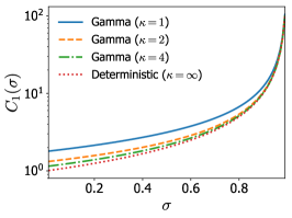
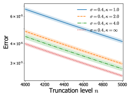
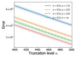
Figure 1: (Left) Constant $C_{1}(\sigma)$ for deterministic and gamma arrival times; (Middle-Right) Simulated error $R_{n}$ with gamma arrival times for (Middle) stable process and (Right) GGP.

5.2 $L_{1}$ error on the marginal likelihood

In this section we discuss the $L_{1}$ error on the marginal likelihood when truncated CRMs are used for hierarchical Bayesian models under the framework described in [16]. Let $W\sim\operatorname*{CRM}(\rho,\mu_{w})$, and $W_{n}$ be its approximation with $n$ atoms. Let $H(\cdot|w)$ be a probability distribution on $\mathbb{N}\cup\{0\}$ for all $w$, and denote $\pi(w):=H(0|w)$. Consider a hierarchical Bayesian model for $m$ observations $X_{1:m}:=\{X_{j}\}_{j=1}^{m}$, $Z_{j}|w_{j}\sim H(w_{j}),\quad X_{j}|z_{j}\sim F(z_{j}),\quad j=1,\dots,m,$ and denote $p_{m,\infty}(X_{1:m})$ the marginal likelihood for this model. Similarly, denote $p_{m,n}(X_{1:m})$ be the marginal likelihood of the model with the same generative process, except for $W_{n}$ instead of $W$. Following [16], we analyze the quality of approximation by comparing $p_{m,\infty}(X_{1:m})$ and $p_{m,n}(X_{1:m})$. For the inverse Lévy case, one recovers the bound derived in [16, Theorem D.3.].

Proposition 5.3.

We have the bound $0\leq\frac{1}{2}||p_{m,\infty}(X_{1:m})-p_{m,n}(X_{1:m})||\leq 1-e^{-B_{m,n}}$, where $B_{m,n}\leq m\int_{0}^{\infty}\int_{0}^{\infty}(1-\pi(w))(1-\Lambda_{w}(\Psi^{-1}(\xi))\rho(dw)\operatorname{Gamma}(\xi;n+1,1)d\xi$.

6 Discussion

Our series construction can be seen as a special case of Rosinski’s shot-noise series representation [52] (as is the case for most series constructions, see [52]), using the disintegration $\rho(dw)=\int_{0}^{\infty}\nu(\xi,dw)d\xi$ where $\nu(\xi,dw)=\lambda_{w}(\Psi^{-1}(\xi))\rho(dw)/\psi(\Psi^{-1}(\xi))$ is a Markov kernel (noting that $\int_{0}^{\infty}\lambda_{w}(\Psi^{-1}(\xi))/\psi(\Psi^{-1}(\xi)))d\xi=1$). [29] proposed alternative ways of deriving iid approximations for some classes of CRMs. The approach does not rely on a latent Poisson construction and is therefore different from the approach considered here. We emphasize that the finite iid construction is useful for both simulation and hierarchical Bayesian modeling in various contexts. Using B.2, one can approximate infinite-dimensional priors with finite-dimensional iid distributions without any numerical inversion. See Appendix G where we discuss an example of our construction applied to normalized GGP mixture models.

Appendix A Background on regular variation and Mellin transforms

This background material comes from the book of [8].

A.1 Definitions

Definition A.1 (Slowly varying function).

A function $\ell:(0,\infty)\to(0,\infty)$ is slowly varying at infinity if for all $c>0$,

$$\frac{\ell(cx)}{\ell(x)}\to 1\textrm{ as }x\to\infty.$$ (20)

Definition A.2 (Regularly varying function).

A function $f:(0,\infty)\to(0,\infty)$ is regularly varying at infinity with exponent $\rho\in\mathbb{R}$ if $f(x)=x^{\rho}\ell(x)$ for some slowly varying $\ell$. A function $f$ is regularly varying at 0 if $f(1/x)$ is regularly varying at infinity, i.e., $f(x)=x^{-\rho}\ell(1/x)$ for some $\rho\in\mathbb{R}$ and slowly varying $\ell$.

A.2 Basic theorems for regularly varying functions

Let $U$ be a regularly function with exponent $\rho$ and slowly varying function $\ell$ locally bounded on $(0,\infty)$.

Theorem A.1 (Karamata’s theorem).

[8, Propositions 1.5.8 and 1.5.10]. Suppose that $U(t)\sim t^{\rho}\ell(t)$ as $t\to\infty$.

• When $\rho>-1$,

  $$\int_{0}^{x}U(t)dt\sim\frac{1}{\rho+1}x^{\rho+1}\ell(x)\textrm{ as }x\to\infty.$$

• When $\rho<-1$,

  $$\int_{x}^{\infty}U(t)dt\sim-\frac{1}{\rho+1}x^{\rho+1}\ell(x)\textrm{ as }x\to\infty.$$

Corollary A.1.

This also holds when $U$ is regularly varying at 0. When $\rho<-1$ and $U(s)\sim s^{\rho}\ell(1/s)$ as $s\to 0$,

$$\int_{x}^{\infty}U(s)ds\sim\frac{-1}{\rho+1}x^{\rho+1}\ell(1/x)\textrm{ as }x\to 0.$$

A.3 Generalized Abelian theorem

Definition A.3.

Given a measurable kernel $k:(0,\infty)\rightarrow\infty$ let

$$\check{k}(z)=\int_{0}^{\infty}t^{-z-1}k(t)dt=\int_{0}^{\infty}u^{z-1}k(1/u)du$$

be its Mellin transform, for $z\in\mathbb{C}$ such that the integral converges.

Remark A.1.

If $k(x)$ has a Mellin transform $\check{k}(z)$ which converges in $(z_{1},z_{2})$, then $h(x)=k(1/x)$ has a Mellin transform $\check{h}(z)=k(-z)$ which converges in $(-z_{2},-z_{1})$.

Theorem A.2.

[8, Theorem 4.1.6 page 201] Let the Mellin transform $\check{k}$ of  $k$ converge at least in the strip $\sigma\leq\operatorname{Re}(z)\leq\tau$, where $-\infty<\sigma<\tau<\infty$. Let $\rho\in(\sigma,\tau)$, $\ell$ a slowly varying function, $c\in\mathbb{R}.$ If $f$ is measurable, $f(x)/x^{\sigma}$ is bounded on every interval $(0,a]$ and

$$f(x)\sim cx^{\rho}\ell(x)\text{ as }x\rightarrow\infty$$

then

$$\int_{0}^{\infty}k(x/t)f(t)t^{-1}dt\sim c\check{k}(\rho)x^{\rho}\ell(x)\text{ as }x\rightarrow\infty$$

The next result is a trivial corollary of A.2, considering limits as $x$ tends to $0$.

Corollary A.2.

Let the Mellin transform $\check{k}$ of  $k$ converge at least in the strip $\tau_{1}\leq\operatorname{Re}(z)\leq\tau_{2}$, where $-\infty<\tau_{1}<\tau_{2}<\infty$. Let $\rho\in(\tau_{1},\tau_{2})$, $\ell$ a slowly varying function, $c\in\mathbb{R}.$ If $f$ is measurable, $f(x)x^{-\tau_{2}}$ is bounded on every interval $[a,\infty)$ and

$$f(x)\sim cx^{\rho}\ell(1/x)\text{ as }x\rightarrow 0$$

then

$$\int_{0}^{\infty}k(x/t)f(t)t^{-1}dt\sim c\check{k}(\rho)x^{\rho}\ell(1/x)\text{ as }x\rightarrow 0$$

Proof.

$$\int_{0}^{\infty}k(x/t)f(t)t^{-1}dt =\int_{0}^{\infty}k(xu)f(1/u)u^{-1}du$$

$$=\int_{0}^{\infty}\widetilde{k}(1/(xu))\widetilde{f}(u)u^{-1}du$$

where $\widetilde{f}(x)=f(1/x)$, $\widetilde{f}(x)/x^{-\tau_{2}}$ bounded on every interval $(0,1/a]$ with

$$\widetilde{f}(x)=f(1/x)\sim cx^{-\rho}\ell(x)\text{ as }x\rightarrow\infty$$

and $\widetilde{k}(x)=k(1/x)$ is such that its Mellin transform converges in the strip $-\tau_{2}\leq\operatorname{Re}(z)\leq-\tau_{1}$. A.2 above therefore gives the result. ∎

Appendix B Proofs

B.1 Proof of 3.1

The proof is an adaption of the proof for the size-biased construction in [46, Section 4]. The mean measure $\nu^{\prime}$ of the Poisson random measure $N^{\prime}$ can be expressed as

$$\nu^{\prime}(dw,d\theta,dt) =\rho(dw)\mu_{w}(d\theta)\lambda_{w}(t)dt$$

$$=\psi(t)dt\times\frac{\lambda_{w}(t)\rho(dw)}{\psi(t)}\times\mu_{w}(d\theta)$$

$$=\psi(t)dt\times\phi_{t}(dw)\times\mu_{w}(d\theta)$$

This is the mean measure of a marked Poisson point process, where $(T_{1},T_{2},\ldots)$ are the points of an inhomogeneous Poisson point process with intensity $\psi(t)$, hence admit the representation Equation (11), and the marks $(W_{i},\theta_{i})$ have conditional distribution $\phi_{t}(dw)\mu_{w}(d\theta)$ as shown in Equation (11). Let $(\overline{X}_{n,1}^{\prime},\ldots,\overline{X}_{n,n}^{\prime})=(X^{\prime}_{\pi_{1}},\ldots,X^{\prime}_{\pi_{n}})$ where $\pi_{n}$ is a random permutation of $\{1,\ldots,n\}$, and $\overline{X}_{n,i}^{\prime}=(\overline{T}_{n,i},\overline{W}_{n,i},\overline{\theta}_{n,i})$. By properties of the Poisson process on the real line, the random variables $\overline{T}_{n,1},\ldots,\overline{T}_{n,n}$ are iid given $T_{n+1}=t_{n+1}$, with pdf

$$\frac{\psi(t)\mathds{1}_{\{0<t<t_{n+1}\}}}{\Psi(t_{n+1})}.$$

Hence, given $T_{n+1}=t_{n+1}$, the marks $\overline{W}_{n,i}$ and $\overline{\theta}_{n,i}$ are also iid, with conditional distribution $\varphi_{t_{n+1}}(d\overline{w}_{n,i})\mu_{\overline{w}_{n,i}}(d\overline{\theta}_{n,i})$ where

$$\varphi_{t_{n+1}}(d\overline{w}_{n,i}) =\mathbb{E}\left[\phi_{\overline{T}_{n,i}}(d\overline{w}_{n,i})\mid T_{n+1}=t_{n+1}\right]$$

$$=\int_{0}^{t_{n+1}}\frac{\lambda_{w}(t)\rho(d\overline{w}_{n,i})}{\psi(t)}\frac{\psi(t)}{\Psi(t_{n+1})}dt$$

$$=\frac{\Lambda_{w}(t_{n+1})\rho(d\overline{w}_{n,i})}{\Psi(t_{n+1})}.$$

B.2 Proof of 3.1

The proof is similar to that of [39, Section 3.1]. Let $f:\Theta\rightarrow(0,\infty)$ be a measurable function.

$$\mathbb{E}\left[e^{-\widetilde{G}_{n}(f)}\right] =\mathbb{E}\left[e^{-\sum_{i=1}^{n}\widetilde{W}_{n,i}f(\widetilde{\theta}_{n,i})}\right]$$

$$=\mathbb{E}\left[e^{-\widetilde{W}_{n,1}f(\widetilde{\theta}_{n,1})}\right]^{n}$$

$$=\left(\int_{S}e^{-wf(\theta)}\widetilde{\varphi}_{n}(dw)\mu_{w}(d\theta)\right)^{n}$$

$$=\left(1-\int_{S}(1-e^{-wf(\theta)})\widetilde{\varphi}_{n}(dw)\mu_{w}(d\theta)\right)^{n}$$

$$=\left(1-\frac{1}{n}\int_{S}(1-e^{-wf(\theta)})\Lambda_{w}(\Psi^{-1}(n))\rho(dw)\mu_{w}(d\theta)\right)^{n}$$

Note that $\Lambda_{w}(\Psi^{-1}(n))\leq 1,\forall n$ and $\Lambda_{w}(\Psi^{-1}(n))\rightarrow 1$ as $n$ tends to infinity. By the bounded convergence theorem, we therefore have

$$\int_{S}(1-e^{-wf(\theta)})\Lambda_{w}(\Psi^{-1}(n))\rho(dw)\mu_{w}(d\theta)\rightarrow\int_{S}(1-e^{-wf(\theta)})\rho(dw)\mu_{w}(d\theta)$$

as $n\rightarrow\infty$. Additionally, for any real sequence $(a_{n})_{n\geq 1}$ converging to $a$ we have $(1-{a_{n}}/{n})^{n}\rightarrow e^{-a}$ as $n\rightarrow\infty$. We therefore obtain

$$\mathbb{E}\left[e^{-\widetilde{G}_{n}(f)}\right]\rightarrow\exp\bigg{(}-\int_{S}(1-e^{-wf(\theta)})\rho(dw)\mu_{w}(d\theta)\bigg{)},$$

where the right-handside is equal to the Laplace functional $\mathbb{E}[e^{-G(f)}]$ of the CRM $G\sim\operatorname*{CRM}(\rho,\mu_{w})$ by Campbell’s theorem [38].

B.3 Proof of 5.1

By the marking theorem for Poisson point processes [38, Chapter 5], given $T_{n+1}=t_{n+1}$, the random measure $\sum_{i\mid T_{i}\geq t_{n+1}}\delta_{X_{i}}$ is a Poisson random measure with mean measure $(1-\Lambda_{w}(t_{n+1}))\rho(dw)\mu_{w}(d\theta)$. The result follows from Campbell’s theorem and the fact that $T_{n+1}=\Psi^{-1}(\xi_{n+1})$.

B.4 Proof of 5.2

We state a slightly more general version of 5.2, where the constant $\zeta_{0}$ in Equation (18) can more generally be any slowly varying function $\ell_{0}(1/x)$. We then prove this generalized proposition.

Proposition B.1.

[Slight generalization of 5.2] Assume that the mean measure $\rho(dw)$ is absolutely continuous with respect to the Lebesgue measure with density function $\rho(w)$ such that

$$\rho(w)\sim w^{-1-\sigma}\ell_{0}(1/w)\text{ as }w\rightarrow 0$$ (21)

where $\sigma\in(0,1)$ and $\ell_{0}$ is a slowly varying function. Assume additionally that $\Lambda_{w}(t)=1-k(wt)$ where $k$ is a positive function on $(0,\infty)$ such that its Mellin transform (see A.3) $\check{k}$ converges in some open interval containing $[\sigma-2,\sigma-1]$. Assume additionally that either (i) $k$ is differentiable with derivative $k^{\prime}$ and that the Mellin transform $\check{k}^{\prime}$ of $k^{\prime}$ is defined in some open interval containing $\sigma-1$, or (ii) that $k(x)=\mathds{1}_{\{x\leq 1\}}$. Then we have

$$R_{n}\sim C_{1}(\sigma)n^{1-1/\sigma}\ell_{**}(n)~{}~{}\text{ almost surely as }n\to\infty$$ (22)

where $\ell_{**}$ is some slowly varying function that depends on $\ell_{0}$ and $\sigma$ but not $\lambda_{w}$ and the constant $C_{1}(\sigma)$ is given by $C_{1}(\sigma)=(1-\sigma)^{-1}$ if $k(x)=\mathds{1}_{\{x\leq 1\}}$ and $C_{1}(\sigma)=\frac{\check{k}(\sigma-1)}{(-\check{k}^{\prime}(\sigma-1))^{1-1/\sigma}}$ if $k$ is differentiable, and only depends on the arrival time distribution $\Lambda_{w}$ and $\sigma$.

In order to B.1, we first state the following proposition.

Proposition B.2.

Assume that

$$\overline{\rho}(x)\sim x^{-\sigma}\ell(1/x)\text{ as }x\to 0$$ (23)

where $\sigma\in(0,1)$ and $\ell$ is a slowly varying function. Assume additionally that

$$\Lambda_{w}(t)=1-k(wt)$$ (24)

where $k$ is a positive and differentiable function on $(0,\infty)$, with derivative $k^{\prime}$. Assume that the Mellin transform $\check{k}^{\prime}$ of $k^{\prime}$ is defined in some open interval containing $\sigma-1$. Then

$$\Psi(t)\sim-\check{k}^{\prime}(\sigma-1)t^{\sigma}\ell(t)~{}~{}~{}\text{ and }~{}~{}~{}\Psi^{-1}(t)\sim(-\check{k}^{\prime}(\sigma-1))^{-1/\sigma}t^{1/\sigma}\ell_{*}(t)~{}~{}\text{ as }t\rightarrow\infty$$ (25)

where $\ell_{*}$ is another slowly varying function depending on $\ell$ and $\sigma$, and defined in Equation (28). If $\ell(x)=c$ is constant, then we simply have $\ell_{*}(x)=c^{-1/\sigma}$. In particular, this is the case for both the generalized gamma process and the stable beta process, which verify condition (23) when $\sigma>0$ with $\ell(x)=\frac{\alpha}{\sigma\Gamma(1-\sigma)}$ for the GGP and $\ell(x)=\frac{\alpha}{\sigma B(1-\sigma,c+\sigma)}$ for the SBP.

Proof of B.2.

The assumptions (21) and the first condition in Equation (9) both imply that

$$\lim_{w\rightarrow 0}\Lambda_{w}(t)\overline{\rho}(w)=0.$$

Using integration by parts

$$\Psi(t) =\int_{0}^{\infty}\Lambda_{w}(t)\rho(dw)$$

$$=[\Lambda_{w}(t)\overline{\rho}(w)]_{w=0}^{\infty}+\int_{0}^{\infty}\frac{\partial\Lambda_{w}(t)}{dw}\overline{\rho}(w)dw$$

$$=\int_{0}^{\infty}\frac{\partial\Lambda_{w}(t)}{dw}\overline{\rho}(w)dw.$$

Now assume $\Lambda_{w}(t)=1-k(wt)$ where $k$ is differentiable on $(0,\infty)$. Then

$$\frac{\partial\Lambda_{w}(t)}{dw}=-tk^{\prime}(wt).$$

If the Mellin transform $\check{k}^{\prime}$ of $k^{\prime}$ is defined in some open interval containing $\sigma-1$, then A.2 implies

$$\Psi(t)\sim-\check{k}^{\prime}(\sigma-1)t^{\sigma}\ell(t)$$ (26)

as $t$ tends to infinity. In the case $k(x)=\mathds{1}_{\{x\leq 1\}}$, $k$ is not differentiable, but we have directly

$$\Psi(t)=\overline{\rho}(1/t)\sim t^{\sigma}\ell(t).$$

Now we use inversion formulas for regularly varying function to get the asymptotic regime for $\Psi^{-1}(t)$. Assume $\sigma>0$, then [25, Lemma 22] implies

$$\Psi^{-1}(t)\sim(-\check{k}^{\prime}(\sigma-1))^{-1/\sigma}t^{1/\sigma}\ell_{*}(t)$$ (27)

as $t\rightarrow\infty$, where $\ell_{*}$ is a slowly varying function defined by

$$\ell_{*}(t)=(\ell^{1/\sigma}(t^{1/\sigma}))^{\#}$$ (28)

where $\ell^{\#}$ denotes the de Bruijn conjugate of the slowly varying function $\ell$ [8, Theorem 1.5.13]. Note that $\ell_{*}$ only depends on $\ell$ and $\sigma$, but not the arrival time distribution $\Lambda_{w}(t)$.

∎

Assume that the mean measure $\rho(dw)$ is absolutely continuous with respect to the Lebesgue measure with density function $\rho(w)$ verifying

$$\rho(w)\sim w^{-1-\sigma}\ell_{0}(1/w)\text{ as }w\rightarrow 0,$$ (29)

where $\sigma\in[0,1]$ and $\ell_{0}$ is a slowly varying function. Equation (21) and [8, Proposition 1.5.8] imply that

$$\overline{\rho}(x)\sim x^{-\sigma}\ell(1/x)$$ (30)

as $x$ tends to 0 where $\ell$ is a slowly varying function defined by

$$\ell(1/x)=\left\{\begin{array}[]{ll}\ell_{0}(1/x)/\sigma&\textrm{ if }\sigma>0\\ \int_{x}^{\infty}u^{-1}\ell_{0}(1/u)du&\textrm{ if }\sigma=0\end{array}\right..$$

Assume additionally that $\Lambda_{w}(t)=1-k(wt)$ where $k$ is a positive function on $(0,\infty)$ such that its Mellin transform (see A.3) $\check{k}$ converges in some open interval containing $[\sigma-2,\sigma-1]$. Note that

$$\mathbb{E}[R_{n}\mid T_{n+1}]=\int_{0}^{\infty}w(1-\Lambda_{w}(T_{n+1}))\rho(dw),~{}~{}\mathbb{V}[R_{n}\mid T_{n+1}]=\int_{0}^{\infty}w^{2}(1-\Lambda_{w}(T_{n+1}))\rho(dw).$$

As $T_{n+1}$ tends to infinity almost surely as $n$ tends to infinity, A.2 implies

$$\mathbb{E}[R_{n}\mid T_{n+1}] \sim\check{k}(\sigma-1)T_{n+1}^{\sigma-1}\ell_{0}(T_{n+1})$$ (31)

$$\mathbb{V}[R_{n}\mid T_{n+1}] \sim\check{k}(\sigma-2)T_{n+1}^{\sigma-2}\ell_{0}(T_{n+1})$$ (32)

almost surely as $n$ tends to infinity.

As $T_{n+1}=\Psi^{-1}(\gamma_{n+1})$ where $\gamma_{n+1}\sim n$ almost surely as $n$ tends to infinity, using B.2 we obtain

$$T_{n+1}\sim(-\check{k}^{\prime}(\sigma-1))^{-1/\sigma}n^{1/\sigma}\ell_{*}(n)$$ (33)

almost surely as $n$ tends to infinity. Combining Equation (33) with Equations (31) and (32), we obtain

$$\mathbb{E}[R_{n}\mid T_{n+1}] \sim\frac{\check{k}(\sigma-1)}{(-\check{k}^{\prime}(\sigma-1))^{1-1/\sigma}}n^{1-1/\sigma}\ell_{*}^{\sigma-1}(n)\ell_{0}(t^{1/\sigma}\ell_{*}(n))$$ (34)

$$\mathbb{V}[R_{n}\mid T_{n+1}] \sim\frac{\check{k}(\sigma-2)}{(-\check{k}^{\prime}(\sigma-1))^{1-2/\sigma}}n^{1-2/\sigma}\ell_{*}^{\sigma-2}(n)\ell_{0}(t^{1/\sigma}\ell_{*}(n))$$ (35)

almost surely as $n$ tends to infinity. Note that if $\ell_{0}(t)=\zeta_{0}$ is constant, then all the other slowly varying functions are also constant with

$$\ell(x)=\frac{\zeta_{0}}{\sigma},~{}~{}~{}\ell_{*}(x)=\ell(x)^{-1/\sigma}=\left(\frac{\zeta_{0}}{\sigma}\right)^{-1/\sigma}.$$ (36)

Finally, Equation (22) follows similarly to the proof of [25, Proposition 2]. Using Chebyshev’s inequality

$$\Pr\left(\left|\frac{R_{n}}{\mathbb{E}[R_{n}\mid T_{n+1}]}-1\right|>\epsilon\mid T_{n+1}\right)\leq\frac{\mathbb{V}[R_{n}\mid T_{n+1}]}{\epsilon^{2}\mathbb{E}[R_{n}\mid T_{n+1}]^{2}}$$

Take $a_{n}=n^{2}$. As

$$\frac{\mathbb{V}[R_{n}\mid T_{n+1}]}{\mathbb{E}[R_{n}\mid T_{n+1}]^{2}}\asymp n^{-1},$$

by the Borel-Cantelli lemma, given $T_{n}$,

$$R_{a_{n}}\sim\mathbb{E}[R_{a_{n}}|T_{a_{n}+1}]$$

almost surely as $n\to\infty$. As $R_{n}$ is decreasing, we have, for any $m^{2}\leq n\leq(m+1)^{2}$

$$\frac{R_{(m+1)^{2}}}{\mathbb{E}[R_{m^{2}}\mid T_{m^{2}+1}]}\leq\frac{R_{n}}{\mathbb{E}[R_{n}\mid T_{n+1}]}\leq\frac{R_{m^{2}}}{\mathbb{E}[R_{(m+1)^{2}}\mid T_{(m+1)^{2}+1}]}$$

and it follows by sandwiching that

$$R_{n}\sim\mathbb{E}[R_{n}|T_{n+1}]$$

almost surely as $n\to\infty$. Combining this with Equation (34) gives the final result, with $\ell_{**}$ the slowly varying function defined by

$$\ell_{**}(t)=\ell_{*}^{\sigma-1}(t)\ell_{0}(t^{1/\sigma}\ell_{*}(t)).$$

Note that in the case of the GGP, the different slowly varying functions are all constant functions

$$\ell_{0}(x) =\frac{\alpha}{\Gamma(1-\sigma)}$$ (37)

$$\ell(x) =\frac{\alpha}{\sigma\Gamma(1-\sigma)}$$ (38)

$$\ell_{*}(x) =\ell(x)^{-1/\sigma}=\left(\frac{\alpha}{\sigma\Gamma(1-\sigma)}\right)^{-1/\sigma}$$ (39)

$$\ell_{**}(x) =\left(\frac{\alpha}{\sigma\Gamma(1-\sigma)}\right)^{-1+1/\sigma}\frac{\alpha}{\Gamma(1-\sigma)}=\left(\frac{\alpha}{\Gamma(1-\sigma)}\right)^{1/\sigma}\sigma^{1-1/\sigma}$$ (40)

For the SBP, we have

$$\ell_{0}(x) =\frac{\alpha}{B(1-\sigma,c+\sigma)}$$ (41)

$$\ell(x) =\frac{\alpha}{\sigma B(1-\sigma,c+\sigma)}$$ (42)

$$\ell_{*}(x) =\ell(x)^{-1/\sigma}=\left(\frac{\alpha}{\sigma B(1-\sigma,c+\sigma)}\right)^{-1/\sigma}$$ (43)

$$\ell_{**}(x) =\left(\frac{\alpha}{B(1-\sigma,c+\sigma)}\right)^{1/\sigma}\sigma^{1-1/\sigma}$$ (44)

B.5 Proof of 5.3

From [16], we have the protobound

$$0\leq\frac{1}{2}||p_{N,\infty}(X_{1:N})-p_{N,n}(X_{1:N})||\leq 1-\mathbb{P}(\text{supp}(X_{1:N})\subseteq\text{supp}(G_{n}))$$

In our case,

$$\mathbb{P}(\text{supp}(X_{1:N})\subseteq\text{supp}(G_{n}))$$

$$=\mathbb{E}\left[\prod_{i=n+1}^{\infty}\pi(W_{i})^{N}\right]$$

$$=\mathbb{E}\left[\mathbb{E}\left[e^{N\sum_{i\geq n+1}\log\pi(W_{i})}\mid T_{n+1}\right]\right]$$

$$=\mathbb{E}\left[\exp\left(-\int_{0}^{\infty}(1-e^{N\log\pi(w)})(1-\Lambda_{w}(T_{n+1}))\rho(dw)\right)\right]$$

$$=\int_{0}^{\infty}\exp\left(-\int_{0}^{\infty}(1-\pi(w)^{N})(1-\Lambda_{w}(\Psi^{-1}(\gamma))\rho(dw)\right)\operatorname{Gamma}(\gamma;n+1,1)d\gamma$$

$$\geq\exp\left(-\int_{0}^{\infty}\int_{0}^{\infty}(1-\pi(w)^{N})(1-\Lambda_{w}(\Psi^{-1}(\gamma))\rho(dw)\operatorname{Gamma}(\gamma;n+1,1)d\gamma\right)$$

where the last inequality follows from Jensen’s inequality.

Appendix C Mellin transforms

Table 1: Kernels, Mellin transforms and asymptotic constants for different arrival time distributions

Name	$\Lambda_{w}(t)$	$k(x)$	$\check{k}(-z)$	$k^{\prime}(x)$	$-\check{k^{\prime}}(-z)$	$C_{1}(\sigma)$
Deterministic	$\mathds{1}_{\{t\geq 1/w\}}$	$\mathds{1}_{\{x\leq 1\}}$	$z^{-1}$	–	–	$(1-\sigma)^{-1}$
Exponential	$1-e^{-wt}$	$e^{-x}$	$\Gamma(z)$	$-e^{-x}$	$\Gamma(z)$	$\Gamma(1-\sigma)^{1/\sigma}$
Gamma	$1-\frac{\Gamma(\kappa,\kappa wt)}{\Gamma(\kappa)}$	$\frac{\Gamma(\kappa,x\kappa)}{\Gamma(\kappa)}$	$\frac{\Gamma(z+\kappa)}{z\Gamma(\kappa)\kappa^{z}}$	$\frac{-\kappa^{\kappa}x^{\kappa-1}e^{-\kappa x}}{\Gamma(\kappa)}$	$\frac{\kappa^{1-z}\Gamma(\kappa+z-1)}{\Gamma(\kappa)}$	$\frac{(\kappa-\sigma)\Gamma(\kappa-\sigma)^{1/\sigma}}{(1-\sigma)\Gamma(\kappa)^{1/\sigma}}$
Inv. gamma	$\frac{\Gamma(\kappa,\kappa/(wt))}{\Gamma(\kappa)}$	$\frac{\gamma(\kappa,\kappa/x)}{\Gamma(\kappa)}$	$\frac{\Gamma(\kappa-z)}{z\Gamma(\kappa)\kappa^{-z}}$	$-\frac{\kappa^{\kappa}e^{-\kappa/x}}{x^{\kappa+1}\Gamma(\kappa)}$	$\frac{\kappa^{z-1}\Gamma(-z+\kappa+1)}{\Gamma(\kappa)}$	$\frac{\Gamma(\kappa+\sigma)^{1/\sigma}}{(1-\sigma)(\kappa+\sigma-1)\Gamma(\kappa)^{1/\sigma}}$
Gen. Pareto	$1-(1+wt)^{-c}$	$(1+x)^{-c}$	$B(z,c-z)$	$-c(1+x)^{-c-1}$	$cB(z,c+1-z)$	$\frac{B(1-\sigma,c+\sigma-1)}{(cB(1-\sigma,c+\sigma))^{1-1/\sigma}}$

C.1 Deterministic kernel

Take $k(t)=\mathds{1}_{\{t\leq 1\}}.$ Then

$$\check{k}(z)=\int_{0}^{\infty}t^{-z-1}k(t)dt=\int_{0}^{1}t^{-z-1}=-z^{-1}$$

if $z<0$.

C.2 Gamma kernel

Take $k(t)=\frac{\Gamma(\kappa,\kappa t)}{\Gamma(\kappa)}$ for $\kappa\geq 1$.

$$\check{k}(z) =\int_{0}^{\infty}u^{-z-1}k(u)du$$

$$=\frac{1}{\Gamma(\kappa)}\int_{0}^{\infty}u^{-z-1}\int_{\kappa u}^{\infty}v^{\kappa-1}e^{-v}dvdu$$

$$=\frac{1}{\Gamma(\kappa)}\int_{0}^{\infty}\int_{0}^{v/\kappa}u^{-z-1}v^{\kappa-1}e^{-v}dudv$$

$$=\frac{-\kappa^{z}}{z\Gamma(\kappa)}\int_{0}^{\infty}v^{\kappa-z-1}e^{-v}dv$$

$$=\frac{-\Gamma(\kappa-z)\kappa^{z}}{z\Gamma(\kappa)}$$

which converges for $z<0$. Additionally, $k^{\prime}(t)=-\frac{\kappa^{\kappa}t^{\kappa-1}e^{-\kappa t}}{\Gamma(\kappa)}$ hence

$$\check{k^{\prime}}(z) =-\int_{0}^{\infty}t^{-z-1}k^{\prime}(t)dt$$

$$=-\frac{\kappa^{\kappa}}{\Gamma(\kappa)}\int_{0}^{\infty}t^{\kappa-z-2}e^{-\kappa t}dt$$

$$=-\frac{\Gamma(\kappa-z-1)\kappa^{z+1}}{\Gamma(\kappa)}$$

which converges for $z<\kappa-1$.

C.3 Inverse gamma kernel

Take $k(t)=\frac{\gamma(\kappa,\kappa/t)}{\Gamma(\kappa)}$. Note that if $\kappa=1$, $k(t)=(1-e^{-1/t})$. Then

$$\check{k}(z) =\int_{0}^{\infty}t^{-z-1}k(t)dt$$

$$=\int_{0}^{\infty}u^{z-1}k(1/u)du$$

$$=\int_{0}^{\infty}u^{z-1}\frac{\gamma(\kappa,\kappa u)}{\Gamma(\kappa)}du$$

$$=\frac{1}{\Gamma(\kappa)}\int_{0}^{\infty}u^{z-1}\int_{0}^{\kappa u}v^{\kappa-1}e^{-v}dvdu$$

$$=\frac{1}{\Gamma(\kappa)}\int_{0}^{\infty}v^{\kappa-1}e^{-v}\int_{v/\kappa}^{\infty}u^{z-1}dudv$$

$$=-\frac{1}{z\Gamma(\kappa)\kappa^{z}}\int_{0}^{\infty}v^{\kappa+z-1}e^{-v}dv\text{ if }z<0$$

$$=-\frac{\Gamma(\kappa+z)}{z\Gamma(\kappa)\kappa^{z}}\text{ if }\kappa+z>0$$

therefore defined for $z\in(-\kappa,0)$. Note that

$$\check{k}(z)\sim-1/z$$

as $\kappa$ tends to infinity, which corresponds to the inverse-Lévy case.

We have

$$k^{\prime}(t)=-\frac{\kappa^{\kappa}}{t^{\kappa+1}\Gamma(\kappa)}e^{-\kappa/t}$$

and

$$\check{k^{\prime}}(z) =\int_{0}^{\infty}t^{-z-1}k^{\prime}(t)dt$$

$$=\int_{0}^{\infty}u^{z-1}k^{\prime}(1/u)du$$

$$=-\frac{\kappa^{\kappa}}{\Gamma(\kappa)}\int_{0}^{\infty}u^{z+\kappa}e^{-\kappa u}du$$

$$=-\frac{\kappa^{-z-1}\Gamma(z+\kappa+1)}{\Gamma(\kappa)}$$

defined for $z\in(-1-\kappa,\infty)$. Note again that $\check{k^{\prime}}(z)\rightarrow-1$ as $\kappa\rightarrow\infty$ (inverse Lévy case).

C.4 Generalized Pareto kernel

Take $k(t)=\frac{1}{(t+1)^{c}}$. Then

$$\check{k}(z) =\int_{0}^{\infty}\frac{t^{-z-1}}{(t+1)^{c}}dt=B(-z,c+z)$$

for $z\in(-c,0)$. We have $k^{\prime}(t)=-\frac{c}{(t+1)^{c+1}}$ hence

$$\check{k^{\prime}}(z) =-c\int_{0}^{\infty}\frac{t^{-z-1}}{(t+1)^{c+1}}dt=-cB(-z,c+1+z)$$

defined for $z\in(-c-1,0)$.

Appendix D BFRY and related distributions

D.1 BFRY distribution

The BFRY distribution, first named in [20] after the work of Bertoin, Fujita, Roynette, and Yor [7], arises much earlier in various contexts [47, 58]. Recently it was highlighted in [39] as a finite-dimensional approximate distribution for stable, generalized gamma, and special case of stable-beta processes. The density of a BFRY distribution with parameter $\sigma<(0,1)$ is written as

$$\operatorname*{BFRY}(dw;\sigma)=\frac{\sigma w^{-1-\sigma}(1-e^{-w})dw.}{\Gamma(1-\sigma)}$$

One can easily verify that the distribution can be simulated as a ratio of independent gamma and beta random variables.

$$G\sim\operatorname{Gamma}(1-\sigma,1),\quad B\sim\operatorname{Beta}(\sigma,1),\quad\frac{G}{B}\overset{d}{=}\operatorname*{BFRY}(\sigma).$$

D.2 Exponentially-tilted BFRY distribution

In [39, 34], the exponentially-tilted version of BFRY distribution was discussed. The density of exponentially-tiled random variable with parameters $\sigma\in(0,1)$, $c>0$ and $\tau>0$ is

$$\operatorname*{etBFRY}(dw;\sigma,t,\tau)=\frac{\sigma w^{-1-\sigma}e^{-\tau w}(1-e^{-tw})dw}{\Gamma(1-\sigma)((t+\tau)^{\sigma}-\tau^{\sigma})}.$$

Then it is easy to show that

$$G\sim\operatorname{Gamma}(1-\sigma,1),\quad U\sim\operatorname{Unif}(0,1),\quad G\cdot((t+\tau)^{\sigma}(1-U)+\tau^{\sigma}U)^{-\frac{1}{\sigma}}\overset{d}{=}\operatorname*{etBFRY}(\sigma,t,\tau).$$

D.3 Generalized BFRY distribution

The generalized BFRY distribution, first discussed in [5], is obtained by generalizing the sampling procedure of BFRY distribution. The generalized BFRY distribution with parameter $\sigma\in(0,1)$ and $\kappa>\sigma$ is obtained as

$$G\sim\operatorname{Gamma}(\kappa-\sigma,1),\quad B\sim\operatorname{Beta}(\sigma,1),\quad\frac{G}{B}\overset{d}{=}\operatorname*{gBFRY}(\kappa,\sigma).$$

By a simple algebra, we obtain the density as

$$\operatorname*{gBFRY}(dw;\kappa,\sigma)=\frac{\sigma w^{-1-\sigma}\gamma(\kappa,w)dw}{\Gamma(\kappa-\sigma)},$$

where $\gamma(\cdot,\cdot)$ is the lower incomplete gamma function.

D.4 Exponentially-tilted generalized BFRY distribution

The density of exponentially-tilted generalized BFRY distribution with parameter $\sigma\in(0,1),\kappa>\sigma,t>0$ and $\tau>0$ is

$$\operatorname*{etgBFRY}(dw;\kappa,\sigma,t,\tau)=\frac{w^{-\sigma-1}e^{-\tau w}\gamma(\kappa,tw)}{\tau^{\sigma}\Gamma(\kappa-\sigma)B_{\frac{t}{t+\tau}}(\kappa,-\sigma)},$$

where $B_{x}(\cdot,\cdot)$ is the incomplete beta function. A random variable having this distribution can be simulated by rejection sampling. Alternatively, note that

$$\operatorname*{etgBFRY}(w;\kappa,\sigma,t,\tau) \propto w^{-\sigma-1}e^{-\tau w}\gamma(\kappa,tw)$$

$$=\sum_{j=0}^{\infty}\frac{\Gamma(\kappa)(tw)^{j+1}e^{-tw}}{\Gamma(\kappa+j+1)}w^{-\sigma-1}e^{-\tau w}$$

$$=\sum_{j=0}^{\infty}\frac{\Gamma(\kappa)}{\Gamma(\kappa+j+1)}t^{\kappa+j}w^{\kappa+j-\sigma-1}e^{-(t+\tau)w}$$

$$=\sum_{j=0}^{\infty}\frac{t^{\kappa+j}\Gamma(\kappa)\Gamma(\kappa+j-\sigma)}{(t+\tau)^{\kappa+j-\sigma}\Gamma(\kappa+j+1)}\operatorname{Gamma}(w;\kappa+j-\sigma,t+\tau).$$

which means that the distribution is an infinite mixture of gamma distributions with mixing proportion

$$\frac{\Gamma(\kappa)(t+\tau)^{\sigma}}{\tau^{\sigma}\Gamma(\kappa-\sigma)B_{\frac{t}{t+\tau}}(\kappa,-\sigma)}\times\bigg{(}\bigg{(}\frac{t}{t+\tau}\bigg{)}^{\kappa+j}\frac{\Gamma(\kappa+j-\sigma)}{\Gamma(\kappa+j+1)}\bigg{)}_{j\geq 1}.$$

Hence, sampling is straightforward as first sampling the component $j$ from above infinite discrete distribution and sampling from corresponding gamma distribution.

The expoentially-tilted GBFRY distribution has a nice property to be a conjugate prior for Poisson, gamma, normal with fixed mean, and Pareto. Let $W\sim\operatorname*{etgBFRY}(\kappa,\sigma,t,\tau)$. Then, for Poisson,

$$X|W\sim\mathrm{Poisson}(\lambda W)\Rightarrow W|X\sim\operatorname*{etgBFRY}(\kappa,\sigma-X,t,\tau+\lambda).$$

For gamma,

$$X|W\sim\operatorname{Gamma}(a,W)\Rightarrow W|X\sim\operatorname*{etgBFRY}(\kappa,\sigma-a,t,\tau+X).$$

For normal,

$$X|W\sim{\mathcal{N}}(\mu,1/W)\Rightarrow W|X\sim\operatorname*{etgBFRY}\bigg{(}\kappa,\sigma-\frac{1}{2},t,\tau+\frac{(X-\mu)^{2}}{2}\bigg{)}.$$

For Pareto,

$$X|W\sim\mathrm{Pareto}(x_{0},W)\Rightarrow W|X\sim\operatorname*{etgBFRY}(\kappa,\sigma-1,t,\tau+\log(X/x_{0})).$$

D.5 Inverse generalized BFRY

One can also consider the counterpart of generalized BFRY distribution where gamma is replaced with inverse gamma. We define inverse generalized BFRY distribution, whose pdf is written as

$$\operatorname*{igBFRY}(w;\kappa,\sigma) =\frac{\sigma}{\Gamma(\kappa+\sigma)}w^{-1-\sigma}\Gamma(\kappa,w^{-1})$$

$$=\frac{\sigma}{\Gamma(\kappa+\sigma)}\int_{1}^{\infty}w^{-\kappa-\sigma-1}v^{\kappa-1}e^{-v/w}dv$$

$$=\int_{1}^{\infty}v^{-1}\cdot\frac{(w/v)^{-\kappa-\sigma-1}e^{-v/w}}{\Gamma(\kappa+\sigma)}\cdot\sigma v^{-\sigma-1}$$

$$=\int_{0}^{1}u\cdot\operatorname{iGamma}(wu;\kappa+\sigma,1)\cdot\operatorname{Beta}(u;\sigma,1)du.$$

Hence, one can realize that

$$G\sim\operatorname{iGamma}(\kappa+\sigma,1),\quad B\sim\operatorname{Beta}(\sigma,1),\quad\frac{G}{B}\overset{d}{=}\operatorname*{igBFRY}(\kappa,\sigma).$$

This distribution corresponds to the truncated exchangeable density $\varphi_{t}(w)$ of stable process with inverse gamma arrival times.

D.6 Exponentially-tilted inverse generalized BFRY

Finally, we consider an exponentially tilted version of inverse GBFRY distribution, whose pdf is written as

$$\operatorname*{etigBFRY}(w;\kappa,\sigma,t,\tau)\propto w^{-1-\sigma}e^{-\tau w}\Gamma(\kappa,(tw)^{-1}).$$

Unfortunately, we don’t have an analytic expression for the normalization constant. We can still sample from this distribution via rejection sampling. This distribution arises as the truncated exchangeable density $\varphi_{t}(w)$ of generalized gamma process with inverse gamma arrival times.

Appendix E Detailed derivations of the results in Section 4 and additional examples

E.1 Exponential arrival times

Generalized gamma.

In the case of the size measure (4) with $\alpha>0,\sigma\in(0,1)$ and $\tau\geq 0$, we have

$$\Psi(t)=\frac{\alpha}{\sigma}\{(t+\tau)^{\sigma}-\tau^{\sigma}\},\quad\psi(t)=\frac{\alpha}{(\tau+\sigma)^{1-\sigma}}.$$

The arrival times are thus generated as

$$T_{i}=\Psi^{-1}(\xi_{i})=\bigg{(}\frac{\sigma}{\alpha}\xi_{i}+\tau^{\sigma}\bigg{)}^{\frac{1}{\sigma}}-\tau.$$

The conditional distribution for the sequential construction is

$$\phi_{t}(dw)=\operatorname{Gamma}(w;1-\sigma,t+\tau)dw.$$

In summary, the sequential construction for the GGP, is given by

$$W_{i}\mid\xi_{i}\sim\operatorname{Gamma}\Bigg{(}1-\sigma,\bigg{(}\frac{\sigma}{\alpha}\xi_{i}+\tau^{\sigma}\bigg{)}^{\frac{1}{\sigma}}\Bigg{)}.$$ (45)

Comparison to Rosinski’s series representation for the GGP

Rosinski [51, 53] proposed the following series representation for the GGP/tempered stable process

$$W_{i}=\min\left(\left(\frac{\xi_{i}\sigma\Gamma(1-\sigma)}{\alpha}\right)^{-1/\sigma},e_{i}u_{i}^{1/\sigma}\right)$$

where $e_{i}\overset{iid}{\sim}\operatorname{Exp}(\tau)$,$u_{i}\overset{iid}{\sim}\operatorname{Unif}(0,1)$. For $i$ large, $W_{i}=\left(\frac{\xi_{i}\sigma\Gamma(1-\sigma)}{\alpha}\right)^{-1/\sigma}$ with high probability, which corresponds to the inverse-Lévy construction for the stable process, and this construction has the same asymptotic error rate as the inverse-Lévy construction for the GGP. The asymptotic error of Rosinski’s representation is therefore lower than the asymptotic error for the series defined by Eq. 45, by a factor $\Gamma(1-\sigma)^{1/\sigma}(1-\sigma)\in(1,2)$, according to Table 1.

E.2 Gamma arrival times

Generalized gamma. Consider the generalized gamma process with (4), $\alpha>0$, $\sigma\in(0,1)$ and $\tau\geq 0$. We have

$$\psi(t) =\int_{0}^{\infty}\frac{\kappa^{\kappa}w^{\kappa}t^{\kappa-1}e^{-\kappa wt}}{\Gamma(\kappa)}\cdot\frac{\alpha}{\Gamma(1-\sigma)}w^{-\sigma-1}e^{-\tau w}dw$$

$$=\frac{\alpha\kappa^{\sigma}\Gamma(\kappa-\sigma)}{\Gamma(\kappa)\Gamma(1-\sigma)}\frac{t^{\kappa-1}}{(t+\tau/\kappa)^{\kappa-\sigma}}$$

$$\Psi(t) =\int_{0}^{t}\psi(s)ds$$

$$=\frac{\alpha\kappa^{\sigma}\Gamma(\kappa-\sigma)}{\Gamma(\kappa)\Gamma(1-\sigma)}\int_{0}^{t}\frac{s^{\kappa-1}}{(s+\tau/\kappa)^{\kappa-\sigma}}ds$$

$$=\left\{\begin{array}[]{ll}\frac{\alpha\tau^{\sigma}\Gamma(\kappa-\sigma)}{\Gamma(\kappa)\Gamma(1-\sigma)}B_{\frac{\kappa t}{\kappa t+\tau}}(\kappa,-\sigma)&\text{if }\tau>0\\ \frac{\alpha\kappa^{\sigma}\Gamma(\kappa-\sigma)}{\sigma\Gamma(\kappa)\Gamma(1-\sigma)}t^{\sigma}&\text{if }\tau=0\end{array}\right.$$

where $B_{x}(a,b)$ is the incomplete beta function. For $\tau=0$, $\Psi^{-1}$ has the analytic expression

$$\Psi^{-1}(\xi)=\bigg{(}\frac{\sigma\Gamma(\kappa)\Gamma(1-\sigma)\xi}{\alpha\kappa^{\sigma}\Gamma(\kappa-\sigma)}\bigg{)}^{\frac{1}{\sigma}}.$$

For $\tau>0$, there is no analytic expression for $\Psi^{-1}$. For the sequential construction, we get

$$\phi_{t}(dw)=\operatorname{Gamma}(w;\kappa-\sigma,\kappa t+\tau)dw.$$

For the exchangeable and iid constructions, we obtain

$$\varphi_{t}(dw)=\left\{\begin{array}[]{ll}\frac{w^{-\sigma-1}e^{-\tau w}\gamma(\kappa,\kappa tw)}{\tau^{\sigma}\Gamma(\kappa-\sigma)B_{\frac{\kappa t}{\kappa t+\tau}}(\kappa,-\sigma)}dw&\text{if }\tau>0\\ \frac{\sigma w^{-1-\sigma}\gamma(\kappa,\kappa tw)}{(\kappa t)^{\sigma}\Gamma(\kappa-\sigma)}&\text{if }\tau=0\\ \end{array}\right.$$

When $\tau=0$, $\varphi_{t}(dw)$ is the distribution of a generalized BFRY distribution (Section D.3). When $\tau>0$, $\varphi_{t}(dw)$ corresponds to the distribution of exponentially-tilted generalized BFRY (Section D.4).

E.3 Inverse gamma arrival times

Take

$$\lambda_{w}(dt)=\operatorname{iGamma}(t;\kappa,\kappa/w)dt.$$

Stable process.

Consider the stable process with size measure (4), $\alpha>0$, $\sigma\in(0,1)$ and $\tau=0$. We have

$$\psi(t)=\frac{\alpha\Gamma(\kappa+\sigma)}{\kappa^{\sigma}\Gamma(1-\sigma)\Gamma(\kappa)t^{1-\sigma}},\quad\Psi(t)=\frac{\alpha\Gamma(\kappa+\sigma)t^{\sigma}}{\sigma\kappa^{\sigma}\Gamma(1-\sigma)\Gamma(\kappa)},\quad T_{i}=\bigg{(}\frac{\sigma\kappa^{\sigma}\Gamma(\kappa)\Gamma(1-\sigma)\gamma_{i}}{\alpha\Gamma(\kappa+\sigma)}\bigg{)}^{\frac{1}{\sigma}}.$$

For the sequential construction, we have

$$\phi_{t}(dw)=\operatorname{iGamma}(dw;\kappa+\sigma,\kappa/t).$$

For the exchangeable construction, we get

$$\varphi_{t}(dw)=\frac{\sigma\kappa^{\sigma}}{t^{\sigma}\Gamma(\kappa+\sigma)}w^{-1-\sigma}\Gamma\bigg{(}\kappa+\sigma,\frac{\kappa}{tw}\bigg{)}.$$

which correspond to inverse generalized BFRY distribution. We can sample from this as $x\sim\operatorname{iGamma}(\kappa+\sigma,1),y\sim\operatorname{Beta}(\sigma,1),w=\frac{\kappa x}{ty}$. See Section D.5 for more details.

The case $\kappa=1$ is of particular interest, as it leads to a tractable novel representation for the GGP, and provide a novel way of interpreting the classical iid approximation of the beta process.

Generalized gamma process.

Consider GGP with size measure (4) with $\alpha>0,\sigma\in[0,1)$ and $\tau>0$. Take inverse gamma arrival time with $\kappa=1$. We have

$$\psi(t)=\frac{2\alpha(\tau t)^{\frac{\sigma+1}{2}}K_{-\sigma-1}(2\sqrt{\tau/t})}{t^{2}\Gamma(1-\sigma)},\quad\Psi(t)=\frac{2\alpha(\tau t)^{\frac{\sigma}{2}}K_{-\sigma}(2\sqrt{\tau/t})}{\Gamma(1-\sigma)},$$ (46)

where $K_{\nu}(\cdot)$ is a modified Bessel function of the second kind. Unfortunately, the arrival time is not given analytically, so we may resort to a numerical root finding algorithm to compute $T_{i}=\Psi^{-1}(\xi_{i})$. The sequential construction is then given by

$$\phi_{t}(dw)=\frac{(\tau t)^{\frac{-\sigma-1}{2}}w^{-\sigma-2}e^{-\tau w-\frac{1}{wt}}dw}{2K_{-\sigma-1}(2\sqrt{\tau/t})}=\operatorname{GIG}(dw;-\sigma-1,2\tau,2/t),$$ (47)

where $\operatorname{GIG}(p,a,b)$ is a generalized inverse Gaussian distribution with parameters $p\in{\mathbb{R}},a>0,b>0$. The exchangeable construction is given by

$$\varphi_{t}(w)=\frac{(\tau t)^{-\frac{\sigma}{2}}w^{-\sigma-1}e^{-\tau w-\frac{1}{wt}}dw}{2K_{-\sigma}(2\sqrt{\tau/t})}=\operatorname{GIG}(dw;-\sigma,2\tau,2/t).$$ (48)

This particular case, which seems to be novel to the best of our knowledge, is useful because it covers the gamma process ($\sigma=0$). It also includes the stable process $(\tau=0)$ as its limiting case - as $\tau\to 0$,

$$\phi_{t}(dw)\to\operatorname{iGamma}(dw;\sigma+1,1/t),\quad\varphi_{t}(w)\to\operatorname{iGamma}(dw;\sigma,1/t).$$ (49)

The sequential construction is impractical since we have to invert $\Psi$ for each $t_{i}$, but the exchangeable construction requires only one inversion for $t_{n+1}$.

Beta process.

Consider the beta process:

$$\rho(dw)=\alpha w^{-1}\mathds{1}_{\{0<w<1\}}dw,$$ (50)

Take the bijective transformation $u=-(\alpha\log(w))^{-1}$ which gives the measure on $(0,\infty)$

$$\rho(du)=u^{-2}du$$ (51)

Note that $\rho(du)$ is not a Lévy measure. Using the inverse gamma kernel with $\kappa=1$ to obtain a series approximation for $\rho(du)$, we obtain

$$\Psi(t)=\int_{0}^{\infty}w^{-2}e^{-1/(wt)}dw=t$$ (52)

and for the iid model we have $\widetilde{U}_{i}\sim\widetilde{\phi}_{n}(du)$ where

$$\widetilde{\phi}_{n}(du)=\frac{1}{n}u^{-2}e^{-1/(nu)}du$$

which is the distribution of an inverse gamma random variable with parameter $(1,1/n)$. Setting the inverse transformation $\widetilde{W}_{i}=e^{-1/(\alpha\widetilde{U}_{i})}$, we obtain

$$\widetilde{W}_{i}\sim\operatorname{Beta}(\alpha/n,1)$$

which corresponds to the classical iid approximation for the beta process, described in the introduction.

This construction can also be obtained directly with different arrival time distribution. Consider

$$\lambda_{w}(dt)=\frac{-\alpha w^{\frac{\alpha}{t}}\log w}{t^{2}}dt,\quad\Lambda_{w}(t)=w^{\frac{\alpha}{t}}.$$ (53)

A sample from this distribution can be obtained as

$$t^{\prime}\sim\operatorname{Exp}(\log w^{-\alpha}),\quad t=1/t^{\prime}.$$ (54)

Then we have

$$\Psi(t)=t,\quad\psi(t)=1,$$ (55)

and as a result

$$\phi_{t}(dw)=-\frac{\alpha}{t^{2}}w^{\frac{\alpha}{t}-1}\log w\mathds{1}_{\{0<w<1\}}dw,\quad\varphi_{t}(dw)=\frac{\alpha}{t}w^{\frac{\alpha}{t}-1}\mathds{1}_{\{0<w<1\}}dw$$ (56)

A sample from $\phi_{t}(w)$ can be obtained by

$$v\sim\operatorname{Gamma}(2,1/t),\quad w=e^{-v/\alpha},$$ (57)

and the exchangeable construction correspond to the iid beta approximation.

E.4 Generalized Pareto arrival time distribution

Consider the following arrival time distribution,

$$\lambda_{w}(dt)=\frac{cw}{(tw+1)^{c+1}}dt,\quad\Lambda_{w}(t)=1-\frac{1}{(tw+1)^{c}}$$ (58)

where $c>0$.

Stable beta process.

Consider the stable beta process with Lévy measure

$$\rho(dw)=\frac{\alpha}{B(1-\sigma,c+\sigma)}w^{-1-\sigma}(1-w)^{c+\sigma-1}\mathds{1}_{\{0<w<1\}}dw.$$ (59)

With change of variable $v=\frac{w}{1-w}$, we see that

$$\Psi(t) =\int_{0}^{1}\frac{\alpha w^{-1-\sigma}(1-w)^{c+\sigma-1}}{B(1-\sigma,c+\sigma)}\bigg{(}1-\frac{1}{(tw+1)^{c}}\bigg{)}dw$$

$$=\frac{\alpha}{B(1-\sigma,c+\sigma)}\int_{0}^{\infty}v^{-1-\sigma}\Big{(}(1+v)^{-c}-((t+1)v+1)^{-c}\Big{)}dv$$

$$=\frac{\alpha}{\Gamma(c)B(1-\sigma,c+\sigma)}\int_{0}^{\infty}\int_{0}^{\infty}v^{-1-\sigma}e^{-vy}(1-e^{-tyv})\cdot y^{c-1}e^{-y}dydv$$

$$=\frac{\alpha\Gamma(1-\sigma)}{\sigma\Gamma(c)B(1-\sigma,c+\sigma)}\int_{0}^{\infty}((t+1)^{\sigma}-1)\cdot y^{c+\sigma-1}e^{-y}dydv$$

$$=\frac{\alpha c}{\sigma}((t+1)^{\sigma}-1)$$

$$\psi(t) =\alpha c(t+1)^{\sigma-1}.$$

For the sequential model we obtain

$$\phi_{t}(dw)=\frac{w^{-\sigma}(1-w)^{c+\sigma-1}(tw+1)^{-c-1}\mathds{1}_{\{0<w<1\}}dw}{B(1-\sigma,c+\sigma)(t+1)^{\sigma-1}}.$$ (60)

With the change of variable $v=\frac{w}{w-1}$, we see that

$$\phi_{t}(dv) =\frac{1}{B(1-\sigma,c+\sigma)(t+1)^{\sigma-1}}v^{-\sigma}(tv+v+1)^{-c-1}dv$$

$$=\frac{1}{B(1-\sigma,c+\sigma)(t+1)^{\sigma-1}\Gamma(c+1)}\int_{0}^{\infty}v^{-\sigma}y^{c}e^{-tvy-vy-y}dy$$

$$=\int_{0}^{\infty}y\cdot\frac{(t+1)^{1-\sigma}(vy)^{-\sigma}e^{-(t+1)vy}}{\Gamma(1-\sigma)}\cdot\frac{y^{c+\sigma-1}e^{-y}}{\Gamma(c+\sigma)}dy,$$

and thus a sample from $\phi_{t}$ can be obtained as

$$z\sim\operatorname{Gamma}(1-\sigma,1+t),\quad y\sim\operatorname{Gamma}(c+\sigma,1),\quad w=\frac{z/y}{z/y+1}.$$ (61)

For the exchangeable model, we have

$$\varphi_{t}(dw)=\frac{\sigma w^{-1-\sigma}(1-w)^{c+\sigma-1}}{cB(1-\sigma,c+\sigma)((t+1)^{\sigma}-1)}\bigg{(}1-\frac{1}{(tw+1)^{c}}\bigg{)}\mathds{1}_{\{0<w<1\}}dw,$$ (62)

and by a similar calculation we see that a sample from $\varphi_{t}$ can be obtained as

$$z\sim\mathrm{etBFRY}(\sigma,t,1),\quad y\sim\operatorname{Gamma}(c+\sigma,1),\quad w=\frac{z/y}{z/y+1}.$$ (63)

Appendix F Details on simulations and additional results

We are interested in measuring the error $R_{n}|T_{n+1}$, apparently not tractable. Hence, we consider the approximate error $R_{n,\hat{n}}$ defined for $\hat{n}>n$ as

$$R_{n,\hat{n}}=\sum_{i=n}^{\hat{n}}W_{i},$$

where we simulate $(W_{i})_{i=1}^{\hat{n}}$ via sequential constructions. When no analytic expression is available (computing $\Psi^{-1}(t)$ for Gamma arrival times for GGP when $\kappa>1$, computing $\bar{\rho}^{-1}(\xi)$ for the inverse-Lévy for GGP), we resort to numerical inversion algorithm. For each configuration, we first sample a series of arrival time sequences, and conditioned on that sample 100 series of jumps $(W_{i})_{i=1}^{\hat{n}}$ to compute $R_{n,\hat{n}}$. We repeat this procedure 10 times for each arrival time sequence (thus 1,000 jump simulations in total for each configuration) and report the mean and standard deviations. Unless specified otherwise, we use the hyperameters $\alpha=2.0,\tau=1.0$ for Stable Process (SP) and GGP, and set $\hat{n}=10^{4}$. Fig. 1 in the paper reports $R_{n,\hat{n}}$ for SP and GGP.

Fig. 2 shows the approximate errors for gamma and inverse gamma arrival times for SP, and gamma arrival times for GGP. We can observe that the variances quickly approach zero, except for the inverse gamma arrival time with $\kappa=1$ case for which our theory predicts to have infinite variance.

Fig. 3 shows the value of constants $C_{1}(\sigma)$ for gamma and inverse gamma arrival times with varying $\sigma$ and $\kappa$ values. Note that lower $C_{1}(\sigma)$ implies lower expected error $\mathbb{E}[R_{n}|T_{n+1}]$ by 5.2. We found that gamma arrival times exhibit lower $C_{1}(\sigma)$ when $0<\sigma<0.5$, and inverse gamma has lower $C_{1}(\sigma)$ when $0.5<\sigma<1$. This observation is empirically confirmed in Fig. 4.

Finally, we compared the approximate error to asymptotic value of $R_{n}$. In case of gamma arrival times for GGP, according to 5.2, we have

$$R_{n}\sim\frac{(\kappa-\sigma)\Gamma(\kappa-\sigma)^{\frac{1}{\sigma}}}{(1-\sigma)\Gamma(\kappa)^{\frac{1}{\sigma}}}\bigg{(}\frac{\alpha}{\Gamma(1-\sigma)}\bigg{)}\sigma^{1-\frac{1}{\sigma}}n^{1-\frac{1}{\sigma}}.$$ (64)

Fig. 5 compares empirical approximate errors with $\hat{n}=10^{6}$ to (64) with different values of $\sigma$. We fixed $\kappa=1$ here. One can see that the approximate error quickly approaches asymptotic errors.

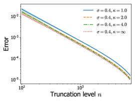
(a) SP-Gamma

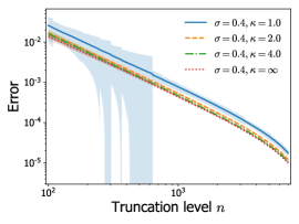
(b) SP-iGamma

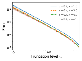
(c) GGP-Gamma

Figure 2: Gamma arrival times, inverse gamma arrival times for stable processes (a-b) and gamma arrival times for GGP (c). Plotted for whole range. See how variances diminishes. Note also that in case of inverse gamma arrival times with $\kappa=1$, the variances diverge as our theory predicts.

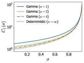
(a) Gamma

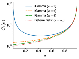
(b) iGamma

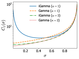
(c) Gamma vs. iGamma

Figure 3: $C_{1}(\sigma)$ values for Gamma (a), inverse gamma (b) arrival times, and comparison between them (c).

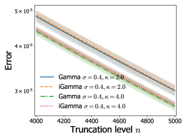
(a) $\sigma=0.4$

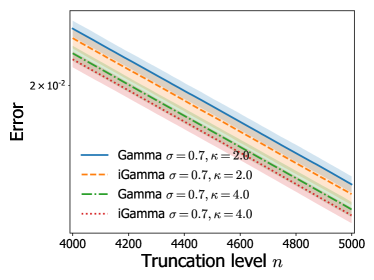
(b) $\sigma=0.7$

Figure 4: Gamma arrival times vs. inverse gamma arrival times for stable process, with $\sigma=0.4$ (a) and $\sigma=0.7$ (b). Gamma is better when $\sigma<0.5$, and inverse gamma is better when $\sigma>0.5$ as predicted in Fig. 3 (c).

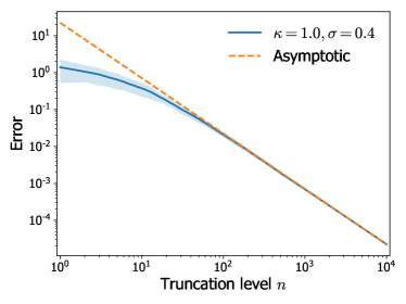
(a) $\sigma=0.4$

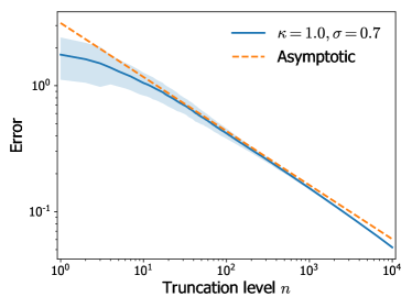
(b) $\sigma=0.7$

Figure 5: Empirical approximation error $R_{n,\hat{n}}$ compared to asymptotic error $R_{n}$, for (a) $\sigma=0.4$ and (b) $\sigma=0.7$.

Appendix G Example on normalized GGP mixture models

Consider a hierarchical Bayesian model

$$G=\sum_{i=1}^{\infty}W_{i}\delta_{\theta_{i}}\sim\operatorname*{CRM}(\rho,H),\,\,\,\theta_{j}\overset{\mathrm{i.i.d.}}{\sim}\frac{G}{G(S)},\,\,\,X_{j}|\theta_{j}\overset{\mathrm{i.i.d.}}{\sim}L(\theta_{j})\textrm{ for }j=1,\dots,m.$$

We approximate infinite dimensional process $G$ with finite iid process $\tilde{G}_{n}$. Then, the rest of the model can be rewritten as

$$Z_{j}|\widetilde{G}_{n}\overset{\mathrm{i.i.d.}}{\sim}\operatorname{Cat}\bigg{(}\frac{\widetilde{w}_{n,i}}{\sum_{i^{\prime}=1}^{n}\widetilde{w}_{n,i^{\prime}}}\bigg{)},\quad X_{j}|z_{j},\widetilde{G}_{n}\overset{\mathrm{i.i.d.}}{\sim}L(\theta_{z_{j}}),$$

We construct $\widetilde{G}_{n}$ via gamma arrival times with $\kappa>1$. Using B.2, we have

$$\widetilde{\varphi}_{n}(w)=\operatorname*{etgBFRY}\bigg{(}w;\kappa,\sigma,\bigg{(}\frac{\sigma\Gamma(\kappa)\Gamma(1-\sigma)n}{\alpha\Gamma(\kappa-\sigma)}\bigg{)}^{\frac{1}{\sigma}},\tau\bigg{)}.$$

Note that we used the function $f(n)=\big{(}\frac{\sigma\Gamma(\kappa)\Gamma(1-\sigma)n}{\alpha\kappa^{\sigma}\Gamma(\kappa-\sigma)}\big{)}^{\frac{1}{\sigma}}$ in place of $\Psi^{-1}(n)$, thus both evaluation of the pdf and sampling can be done without any numerical approximation. The joint density of the mixture model is then written as

$$w_{\bullet}^{-n}\prod_{k=1}^{n}w_{k}^{m_{k}}\widetilde{\varphi}_{n}(w_{k})\bigg{[}\prod_{j:z_{j}=k}\ell(x_{j}|\theta_{k})\bigg{]}h(\theta_{k}),$$

where $\ell$ and $h$ are the density for $L$ and $H$, $w_{\bullet}\vcentcolon=\sum_{i=1}^{n}w_{i}$, and $m_{k}\vcentcolon=\sum_{j=1}^{m}\mathds{1}_{\{z_{j}=k\}}$. Now we are free to any posterior inference algorithm, such as variational inference or stochastic gradient MCMC as in [39].

References

- [1] R. Argiento, I. Bianchini, and A. Guglielmi. A blocked Gibbs sampler for NGG-mixture models via a priori truncation. Statistics and Computing, 26(3):641–661, 2016.
- [2] R. Argiento, I. Bianchini, and A.s Guglielmi. Posterior sampling from -approximation of normalized completely random measure mixtures. Electronic Journal of Statistics, 10(2):3516–3547, 2016.
- AC [19] F. Ayed and F. Caron. Nonnegative Bayesian nonparametric factor models with completely random measures for community detection. arXiv:1902.10693, 2019.
- ADH [10] C. Andrieu, A. Doucet, and R. Holenstein. Particle Markov chain Monte Marlo methods. Journal of the Royal Statistical Society: Series B (Statistical Methodology), 72(3):269–342, 2010.
- ALC [19] F. Ayed, J. Lee, and F. Caron. Beyond the Chinese restaurant and Pitman-Yor processes: statistical models with double power-law behavior. arXiv:1902.04714, 2019.
- AP [17] J. Arbel and I. Prünster. A moment-matching ferguson & klass algorithm. Statistics and Computing, 27(1):3–17, 2017.
- BFRY [06] J. Bertoin, T. Fujita, B. Roynette, and M. Yor. On a particular class of self-decomposable random variables : the durations of Bessel excursions straddling independent exponential times. Probability and Mathematical Statistics, 26(2):315–366, 2006.
- BGT [89] N. H. Bingham, C. M. Goldie, and J. L. Teugels. Regular variation, volume 27. Cambridge university press, 1989.
- BJ [06] D. M. Blei and M. I. Jordan. Variational inference for Dirichlet process mixtures. Bayesian analysis, 1(1):121–143, 2006.
- BLNBP [13] E. Barrios, A. Lijoi, L. E. Nieto-Barajas, and I. Prünster. Modeling with normalized random measure mixture models. Statistical Science, 28(3):313–334, 2013.
- BNS [01] O. E. Barndorff-Nielsen and N. Shephard. Non-Gaussian Ornstein–Uhlenbeck-based models and some of their uses in financial economics. Journal of the Royal Statistical Society: Series B (Statistical Methodology), 63(2):167–241, 2001.
- Bon [82] L. Bondesson. On simulation from infinitely divisible distributions. Advances in Applied Probability, 14(4):855–869, 1982.
- Bri [99] A. Brix. Generalized gamma measures and shot-noise Cox processes. Advances in Applied Probability, 31(4):929–953, 1999.
- Car [12] F. Caron. Bayesian nonparametric models for bipartite graphs. In Advances in Neural Information Processing Systems 25. 2012.
- CCB [16] D. Cai, T. Campbell, and T. Broderick. Edge-exchangeable graphs and sparsity. In D. D. Lee, M. Sugiyama, U. V. Luxburg, I. Guyon, and R. Garnett, editors, Advances in Neural Information Processing Systems 29, pages 4249–4257. Curran Associates, Inc., 2016.
- CCB [18] T. Campbell, D. Cai, and T. Broderick. Exchangeable trait allocations. Electronic Journal of Statistics, 12(2):2290–2322, 2018.
- CF [17] F. Caron and E. Fox. Sparse graphs using exchangeable random measures. Journal of the Royal Statistical Society B, 79:1295–1366, 2017. Part 5.
- CHHB [19] T. Campbell, J. H. Huggins, J. P. How, and T. Broderick. Truncated random measures. Bernoulli, 2019.
- CT [04] R. Cont and P. Tankov. Financial modelling with jump processes, volume 2. CRC press, 2004.
- DJ [14] L. Devroye and L. F. James. On simulation and properties of the stable law. Statistical Methods and Applications, 23(3):307–343, 2014.
- DMVGT [09] F. Doshi, K. Miller, J. Van Gael, and Y. W. Teh. Variational inference for the Indian buffet process. In Artificial Intelligence and Statistics, pages 137–144, 2009.
- FK [72] T. S. Ferguson and M. J. Klass. A representation of independent increment processes without gaussian components. The Annals of Mathematical Statistics, 43(5):1634–1643, 1972.
- FW [12] N. Foti and S. Williamson. Slice sampling normalized kernel-weighted completely random measure mixture models. In Advances in Neural Information Processing Systems, pages 2240–2248, 2012.
- GG [06] Thomas L. Griffiths and Zoubin Ghahramani. Infinite latent feature models and the Indian buffet process. In Advances in Neural Information Processing Systems 18 (NIPS 2005), 2006.
- GHP [07] A. Gnedin, B. Hansen, and J. Pitman. Notes on the occupancy problem with infinitely many boxes: general asymptotics and power laws. Probability surveys, 4:146–171, 2007.
- GRRB [14] P. Gopalan, F. J. Ruiz, R. Ranganath, and D. M. Blei. Bayesian nonparametric Poisson factorization for recommendation systems. In AISTATS, pages 275–283, 2014.
- GW [11] J. E. Griffin and S. G. Walker. Posterior simulation of normalized random measure mixtures. Journal of Computational and Graphical Statistics, 20(1):241–259, 2011.
- Hjo [90] N. L. Hjort. Nonparametric Bayes estimators based on beta processes in models for life history data. The Annals of Statistics, 18(3):1259–1294, 1990.
- HMBM [17] J. Huggins, L. Masoero, T. Broderick, and L. Mackey. Generic finite approximations for practical bayesian nonparametrics. In NIPS Workshop on “Advances in Approximate Bayesian Inference", 2017.
- Hou [86] P. Hougaard. Survival models for heterogeneous populations derived from stable distributions. Biometrika, 73(2):387–396, 1986.
- IJ [01] H. Ishwaran and L. F. James. Gibbs sampling methods for stick-breaking priors. Journal of the American Statistical Association, 96(453):161–173, 2001.
- Jam [05] L. F. James. Bayesian Poisson process partition calculus with an application to Bayesian Lévy moving averages. The Annals of Statistics, 33(4):1771–1799, 2005.
- JLP [09] L. F. James, A. Lijoi, and I. Prünster. Posterior analysis for normalized random measures with independent increments. Scandinavian Journal of Statistics, 36(1):76–97, 2009.
- JOT [15] L. F. James, P. Orbanz, and Y. W. Teh. Scaled subordinators and generalizations of the Indian buffet process. arXiv:1510.07309, 2015.
- Khi [37] A. Khintchine. Zur theorie der unbeschränkt teilbaren verteilungsgesetze. Rec. Math. Moscou, n. Ser, 2:79–117, 1937.
- Kin [67] J. F. C. Kingman. Completely random measures. Pacific Journal of Mathematics, 21(1):59–78, 1967.
- Kin [75] J. F. C. Kingman. Random discrete distributions. Journal of the Royal Statistical Society: Series B (Methodological), 37(1):1–15, 1975.
- Kin [93] J.F.C. Kingman. Poisson processes, volume 3. Oxford University Press, USA, 1993.
- LJC [16] J. Lee, L. F. James, and S. Choi. Finite-dimensional BFRY priors and variational Bayesian inference for power-law models. In Advances in Neural Information Processing Systems 29 (NIPS 2016), 2016.
- LP [10] A. Lijoi and I. Prünster. Models beyond the Dirichlet process. In N. L. Hjort, C. Holmes, P. Müller, and S. G. Walker, editors, Bayesian Nonparametrics. Cambridge University Press, 2010.
- MW [03] J. Moller and R. P. Waagepetersen. Statistical inference and simulation for spatial point processes. Chapman and Hall/CRC, 2003.
- NBPW [04] L. E. Nieto-Barajas, I. Prünster, and S. G. Walker. Normalized random measures driven by increasing additive processes. The Annals of Statistics, 32(6):2343–2360, 2004.
- PBJ [12] J. Paisley, D. Blei, and M.l Jordan. Stick-breaking beta processes and the Poisson process. In Artificial Intelligence and Statistics, pages 850–858, 2012.
- PC [09] J. Paisley and L. Carin. Nonparametric factor analysis with beta process priors. In Proceedings of the 26th Annual International Conference on Machine Learning, pages 777–784. ACM, 2009.
- PCB [11] J. Paisley, L. Carin, and D. Blei. Variational inference for stick-breaking Beta process priors. In ICML, pages 889–896. Citeseer, 2011.
- PPY [92] M. Perman, J. Pitman, and M. Yor. Size-biased sampling of Poisson point processes and excursions. Probability Theory and Related Fields, 92(1):21–39, 1992.
- PY [97] J. Pitman and M. Yor. The two-parameter Poisson-Dirichlet distribution derived from a stable subordinator. The Annals of Probability, 25(2):855–900, 1997.
- RK [15] A. Roychowdhury and B. Kulis. Gamma processes, stick-breaking, and variational inference. In Artificial Intelligence and Statistics, pages 800–808, 2015.
- RLP [03] E. Regazzini, A. Lijoi, and I. Prünster. Distributional results for means of normalized random measures with independent increments. Annals of Statistics, 31(2):560–585, 04 2003.
- Ros [90] J. Rosiński. On series representations of infinitely divisible random vectors. The Annals of Probability, pages 405–430, 1990.
- [51] J. Rosiński. Contribution to the discussion of the paper “Non-Gaussian Ornstein-Uhlenbeck-based models and some of their uses in financial economics” by O. Barndorff-Nielsen and N. Shephard. Journal of the Royal Statistical Society, Series B, 63:230–231, 2001.
- [52] J. Rosiński. Series representations of Lévy processes from the perspective of point processes. In Ole E. Barndoff-Nielson, Thomas Mikosch, and Sidney I. Resnick, editors, Lévy Processes - Theory and Applications, pages 401–415. Birkhäuser, Boston, 2001.
- Ros [07] J. Rosiński. Tempering stable processes. Stochastic processes and their applications, 117(6):677–707, 2007.
- TG [09] Y. W. Teh and D. Gorur. Indian buffet processes with power-law behavior. In Advances in neural information processing systems, pages 1838–1846, 2009.
- TGG [07] Y. W. Teh, D. Grür, and Z. Ghahramani. Stick-breaking construction for the Indian buffet process. In Artificial Intelligence and Statistics, pages 556–563, 2007.
- [56] R. L. Wolpert and K. Ickstadt. Poisson/gamma random field models for spatial statistics. Biometrika, 85(2):251–267, 1998.
- [57] R. L. Wolpert and K. Ickstadt. Simulation of Lévy random fields. In Practical nonparametric and semiparametric Bayesian statistics, pages 227–242. Springer, 1998.
- Win [05] M. Winkel. Electronic foreign-exchange markets and passage events of independent subordinators. Journal of Applied Probability, 42(1):138–152, 2005.
- ZHDC [12] M. Zhou, L. Hannah, D. Dunson, and L. Carin. Beta-negative binomial process and Poisson factor analysis. In Neil D. Lawrence and Mark Girolami, editors, Proceedings of the Fifteenth International Conference on Artificial Intelligence and Statistics, volume 22 of Proceedings of Machine Learning Research, pages 1462–1471, La Palma, Canary Islands, 21–23 Apr 2012. PMLR.
- Zho [15] M. Zhou. Infinite edge partition models for overlapping community detection and link prediction. In Artificial Intelligence and Statistics, pages 1135–1143, 2015.