Maximal Free-Space Concentration of Electromagnetic Waves

Abstract

We derive upper bounds to free-space concentration of electromagnetic waves, mapping out the limits to maximum intensity for any spot size and optical beam-shaping device. For sub-diffraction-limited optical beams, our bounds suggest the possibility for orders-of-magnitude intensity enhancements compared to existing demonstrations, and we use inverse design to discover metasurfaces operating near these new limits. We also demonstrate that our bounds may surprisingly describe maximum concentration defined by a wide variety of metrics. Our bounds require no assumptions about symmetry, scalar waves, or weak scattering, instead relying primarily on the transformation of a quadratic program via orthogonal-projection methods. The bounds and inverse-designed structures presented here can be useful for applications from imaging to 3D printing.

Free-space optical waves with large focal-point intensities and arbitrarily small spot sizes—below the diffraction limit—are a long-sought goal McCutchen (1967); Stelzer (2002); Zheludev (2008) for applications ranging from imaging Gustafsson (2005); Betzig et al. (2006); Rust et al. (2006); Hell (2007); Huang et al. (2008) to 3D printing Lipson and Kurman (2013); Chia and Wu (2015), for which nanostructured lenses have enabled recent experimental breakthroughs Huang and Zheludev (2009); Rogers et al. (2012). In this Letter, we derive upper bounds to free-space concentration of electromagnetic waves, revealing the maximum possible focal-point intensity (related to the well-known “Strehl ratio” Strehl (1902); Born and Wolf (2013)) for a fixed source power and for any desired spot size. For waves incident from any region of space—generated by scattering structures, spatial light modulators, or light sources of arbitrary complexity—we show that the non-convex beam-concentration problem can be transformed to a quadratic program Bertsekas (2016) with easily computable global optima. We also extend this approach to derive maximum intensity independent of the exit surface of an incident wave. Our bounds simplify to those derived by Fourier analysis of prolate spheroidal wave functions Slepian (1961); Landau and Pollak (1961); Ferreira and Kempf (2006) in the scalar 1D limit. By honing in on the two essential degrees of freedom—the field intensity at the focal point, and its average over a ring at the desired spot size—the beam-concentration problem can be further simplified to a rank-two optimization problem, resulting in analytical upper bounds in the far zone. For very small spot sizes $G$, which are most desirable for transformative applications, we show that the focal-point intensity must decrease proportional to $G^{4}$, a dimension-independent scaling law that cannot be overcome through any form of wavefront engineering. The bounds have an intuitive interpretation: the ideal field profile at the exit surface of an optical beam-shaping device must have maximum overlap with the fields radiating from a dipole at the origin yet be orthogonal to the fields emanating from a current loop at the spot size radius. We compare theoretical proposals and experimental demonstrations to our bounds, and we find that there is significant opportunity for order-of-magnitude intensity enhancements at those small spot sizes. We use “inverse design” Jensen and Sigmund (2011); Miller (2012); Bendsoe and Sigmund (2013); Molesky et al. (2018), a large-scale computational-optimization technique, to design metasurfaces that generate nearly optimal wavefronts and closely approach our general bounds. By reformulating the light-concentration problem under alternative spot-size metrics, we show that the ideal field profiles for all these metrics are nearly identical in the far zone, suggesting that our analytical bounds, scaling laws, and ideal field profiles may be even more general than expected.

It is now well-understood that the diffraction “limit,” which is a critical factor underpinning resolution limits in imaging Gustafsson (2005); Betzig et al. (2006); Rust et al. (2006); Hell (2007); Huang et al. (2008), photolithography Kawata et al. (1989); Ito and Okazaki (2000); Odom et al. (2002), and more  Rugar (1984); Indebetouw et al. (2007); Kumar et al. (2012); Collier (2013) (and is highly pertinent for applications such as surface-enhanced Raman scattering (SERS) Moskovits (1985); Nie and Emory (1997); Kneipp et al. (1997) and extraordinary optical transmission (EOT) Ebbesen et al. (1998); Martín-Moreno et al. (2001); Genet and Ebbesen (2007)), is not a strict bound on the size of an optical focal spot, but rather a soft threshold below which beam formation is difficult in some generic sense (e.g., accompanied by high-intensity sidelobes). Although evanescent waves can be leveraged to surpass the diffraction limit Fang et al. (2005); Kostelak et al. (1991); Merlin (2007); Zhang and Liu (2008); Ma et al. (2018), they require structuring in the near field. The possibility of sub-diffraction-limited spot sizes without near-field effects was recognized in 1952 by Toraldo di Francia Toraldo di Francia (1952); stimulated by results on highly-directive antennas Schelkunoff (1943), he analytically constructed successively narrower beam profiles with successively larger sidelobe energies (i.e. energies outside the first zero), in a scalar, weak-scattering asymptotic limit. Subsequent studies Berry (1994a, b); Berry and Popescu (2006); Lindberg (2012) have connected the theory of sub-diffraction-limited beams to “super-oscillations” in Fourier analysis Kempf and Ferreira (2004); Aharonov et al. (2011), i.e. bandlimited functions that oscillate over length/time scales faster than the inverse of their largest Fourier component. For one- and two-dimensional scalar fields, superoscillatory wave solutions have been explicitly constructed Berry and Popescu (2006); Wong and Eleftheriades (2010); Chremmos and Fikioris (2015); Smith and Gbur (2016), and in the one-dimensional case energy-concentration bounds have been derived Ferreira and Kempf (2006) by the theory of prolate spheroidal wave functions Slepian (1961); Landau and Pollak (1961). For optical beams, the only known bounds to focusing (apart from bounds on energy density at a point without considering spot sizes Bassett (1986); Sheppard and Larkin (1994)) are those derived in Refs. Sales and Morris (1997); Liu et al. (2002) (and recently in Rogers et al. (2018), albeit with bounds on related but different quantities), which use special-function expansions and/or numerical-optimization techniques to discover computational bounds that apply for weakly scattering, rotationally symmetric filters in a scalar approximation. A bound that does not require weak scattering was developed in Liu et al. (2002), but it still assumes rotational symmetry in a scalar diffraction theory.

There has been further work towards mapping possible field distributions and the structures that might achieve them. Singular-value decompositions can be used to rigorously identify a basis for all possible “receiver” (e.g., image-plane) field solutions Miller (2019). Then, given a known feasible solution, one can use the equivalence principle via physical polarizabilities to identify practical metasurfaces that achieve such field distributions Pfeiffer and Grbic (2013). However, neither of these approaches is able to identify among all possible Maxwell solutions which ones are optimal.

The recent demonstrations Huang et al. (2007a, b); Dennis et al. (2008); Huang and Zheludev (2009); Wang et al. (2009); Kitamura et al. (2010); Rogers et al. (2012, 2013); Huang et al. (2013, 2014); Qin et al. (2015); Wong and Eleftheriades (2015, 2017) of complex wavelength-scale surface patterns focusing plane waves to sub-diffraction-limited spot sizes have inspired hope that the previous tradeoffs of large sidelobe energies or small focal-point intensities might be circumvented or ameliorated by strongly scattering media accounting for the vector nature of light Wang et al. (2009); Huang et al. (2013), as all previous Berry and Popescu (2006); Ferreira and Kempf (2006); Sales and Morris (1997); Liu et al. (2002) asymptotic scaling relations and energy bounds require assumptions of rotational symmetry, weak scattering (except Liu et al. (2002)), and scalar waves. Such possibilities are especially enticing in the context of the broader emergence of “metasurfaces” Kildishev et al. (2013); Yu and Capasso (2014); Khorasaninejad et al. (2016); Li et al. (2018) enabling unprecedented optical response. Given the importance of polarization filtering and high-numerical-aperture lenses to various imaging modalities, incorporation of the vector nature of light is critical to identifying ultimate resolution limits Serrels et al. (2008); Jabbour and Kuebler (2008); Bauer et al. (2014). Moreover, recent design strategies for (diffraction-limited) metasurface lenses have shown that it is critical to account for strong-scattering physics in order to achieve high-efficiency structures Lin et al. (2019); Chung and Miller (2019), a conclusion that extends to superresolving metalenses as well.

In this Article, we derive bounds on the maximum concentration of light that do apply in the fully vectorial, strongly scattering regime, without imposing any symmetry constraints. Our derivation starts with the electromagnetic equivalence principle Kong (1975), which allows us to consider the effects of any scatterer/modulator/light source as effective currents on some exit surface (Sec. I.1). The optimal beam-concentration problem is non-convex due to the requirement for a particular spot size, but we use standard transformations from optimization theory to rewrite the problem as a quadratic program amenable to computational solutions for global extrema. We subsequently bound the solution to the quadratic problem by a simpler and more general rank-two optimization problem (Sec. I.1), and also develop bounds independent of exit surface via modal decomposition (Sec. I.2). The rank-two bounds reduce to analytic expressions in the far zone, and we compare the ideal field profiles to various theoretical and experimental demonstrations in Sec. II. We show that there is still opportunity for orders-of-magnitude improvements, and design metasurfaces approaching our bounds (Sec. III). We also investigate how our bounds on maximum intensity perform under alternative spot-size metrics in Sec. IV. Finally, in Sec. V, we discuss extensions of our framework to incorporate metrics other than focal-point intensity, near-field modalities, inhomogeneities, new point-spread functions, and more.

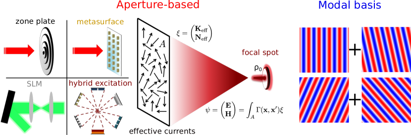
Figure 1: Our framework establishes maximum light concentration for any zero-field contour, such as a circle. We derive two bounds: one that incorporates the shape of the exit aperture (enabling comparison with the well-known Strehl ratio), while otherwise independent of the beam-generation method, and a second that requires only a modal basis and is independent of aperture.

I General Bounds

I.1 Aperture-Dependent Bounds

Consider a beam generated by almost any means, e.g., an incident wave passing through a scatterer with a complex structural profile Levy et al. (2007); Wei et al. (2013); Keren-Zur et al. (2016), precisely controlled spatial light modulators Weiner (2000); Chattrapiban et al. (2003); Guo et al. (2007); Zhu and Wang (2014), or a light source with a complex spatial emission profile Lodahl et al. (2004); Ringler et al. (2008); Bleuse et al. (2011). The physics underlying the extent to which such a beam is spatially concentrated in free space is distilled to its essence by the electromagnetic equivalence principle Kong (1975): the propagating fields are uniquely defined by their tangential values on any beam-generation exit surface, forming effective surface currents that encapsulate the entire complexity of the field-generation process (The surface equivalence principle is the starting point for diffraction theory Born and Wolf (2013) and has been used recently for metasurface-based wavefront shaping Pfeiffer and Grbic (2013); Epstein and Eleftheriades (2016); Ra’di et al. (2017) and optimal antenna designs Gustafsson and Nordebo (2013); Shi et al. (2017)). By this principle, the beam-focusing problem is equivalent to asking: what is the maximum spatial concentration of a beam generated by electric and magnetic surface currents radiating in free space? We depict this distillation of the problem in Fig. 1. We consider fields and currents at a single temporal frequency $\omega$ ($e^{-i\omega t}$ time evolution), and simplify the expressions to follow by encapsulating the electric and magnetic fields ($\mathbf{E}$, $\mathbf{H}$) and currents ($\mathbf{K}_{\rm eff}$, $\mathbf{N}_{\rm eff}$) in 6-vectors $\psi$ and $\xi$, respectively:

$$\psi=\begin{pmatrix}\mathbf{E}\\ \mathbf{H}\end{pmatrix},\quad\xi=\begin{pmatrix}\mathbf{K}_{\rm{eff}}\\ \mathbf{N}_{\rm{eff}}\end{pmatrix}.$$ (1)

The fields $\psi$ emanating from the effective currents $\xi$ distributed across the “exit” surface $A$ are given by the convolution of the currents with $\bm{\Gamma}$, the known $6\times 6$ free-space dyadic Green’s function Chew (1995):

$$\psi(\mathbf{x})=\int_{A}\bm{\Gamma}(\mathbf{x},\mathbf{x}^{\prime})\xi(\mathbf{x}^{\prime}).$$ (2)

Thus, the currents comprise the degrees of freedom determining the beam shape. As illustrated in Fig. 1, finding the maximum focal intensity at a single point for any desired focal spot size now reduces to determining the optimal effective currents. We will assume equations such as Eq. (2) can be solved by any standard electromagnetic discretization scheme Jin (2011), and we will write the matrix versions with the same symbols but without position arguments. For example, $\psi=\bm{\Gamma}\xi$ is the matrix equivalent of Eq. (2), with $\psi$ and $\xi$ vectors and $\bm{\Gamma}$ a matrix. The total intensity at any point in free space, summing electric and magnetic contributions, is given by the squared norm of $\psi$:

$$I(\mathbf{x})= \left|\psi(\mathbf{x})\right|^{2}=\int_{A}\int_{A}\xi^{\dagger}(\mathbf{x}^{\prime\prime})\bm{\Gamma}^{\dagger}(\mathbf{x},\mathbf{x}^{\prime\prime})\bm{\Gamma}(\mathbf{x},\mathbf{x}^{\prime})\xi(\mathbf{x}^{\prime})$$

$$= \xi^{\dagger}\bm{\Gamma}^{\dagger}\bm{\Gamma}\xi.$$ (3)

We now formulate the maximal-concentration question as a constrained optimization problem. The ideal optical beam has maximum focal intensity at a point (set at $\mathbf{x}=0$), zero field along some spot-size contour $\mathcal{C}$, and a total propagating power $P$ not exceeding an input value of $P_{0}$. In Sec. IV we consider alternatives to a zero-field contour as metrics of concentration, thus we denote the optimization problem with the zero-field contour as “(OP_ZF).” Then, the maximum focal intensity, and the ideal effective currents generating it, solve the optimization problem denoted by:

$${\rm(OP_{ZF})}$$ (4)

$$\underset{\xi}{\text{maximize}} I(\mathbf{x}=0)=\xi^{\dagger}\bm{\Gamma}_{0}^{\dagger}\bm{\Gamma}_{0}\xi$$

subject to $$\psi(\mathbf{x})\big{\rvert}_{\mathcal{C}}=\bm{\Gamma}_{\mathcal{C}}\xi=0\quad\textrm{and}\quad P\leq P_{0},$$

where the “0” and $\mathcal{C}$ subscripts indicate that $\bm{\Gamma}$ and $\psi$ are evaluated (in the appropriate basis) at the origin or at the spot-size contour, respectively. (It does not violate any physical laws to set all electric and magnetic components to zero on a contour. If one wanted to require only a subset of field components to be zero then that could be achieved by only including those components in the definition of $\bm{\Gamma}_{\mathcal{C}}$.) Attempting to directly solve Eq. (4) is infeasible: the $\bm{\Gamma}_{0}^{\dagger}\bm{\Gamma}_{0}$ matrix is positive semidefinite (which is nonconvex under maximization Boyd and Vandenberghe (2004)), the equality constraint prevents the use of Rayleigh-quotient-based approaches Horn and Johnson (2013), and the power constraint is difficult to write in a simple convex form.

We can bypass the nonconvexity of the optimization problem, $\rm(OP_{ZF})$, through multiple transformations. First, to simplify the power constraint, we replace it with a constraint on the intensity of the effective currents, normalized such that their total intensity is one: $\xi^{\dagger}\xi=1$. We seek the ideal beam, which has all of its intensity generating power in the direction of the maximum-intensity spot, validating this replacement. Second, we subsume the equality constraint by considering only the effective currents that satisfy zero field on $\mathcal{C}$ by construction. To this end, we project the currents $\xi$ onto the subspace of all currents that generate zero field on $\mathcal{C}$: $\xi=\left(\mathbf{I}-\bm{\Gamma}_{\mathcal{C}}^{\dagger}\left(\bm{\Gamma}_{\mathcal{C}}\bm{\Gamma}_{\mathcal{C}}^{\dagger}\right)^{-1}\bm{\Gamma}_{\mathcal{C}}\right)\nu=\mathbf{P}\nu$, where $\mathbf{I}$ is the identity matrix, the second term is the orthogonal projection matrix Trefethen and Bau III (1997); Bertsekas (2016) for $\bm{\Gamma}_{\mathcal{C}}$, and the $\mathbf{P}$ matrix projects onto the null space of $\bm{\Gamma}_{\mathcal{C}}$ (we have assumed any linearly dependent rows of $\bm{\Gamma}_{\mathcal{C}}$ have been removed such that the inverse of $\bm{\Gamma}_{\mathcal{C}}\bm{\Gamma}_{\mathcal{C}}^{\dagger}$ exists). By this projection, the equality constraint, which sets the field to zero on $\mathcal{C}$, is satisfied for arbitrary effective currents $\xi$: $\bm{\Gamma}_{\mathcal{C}}\xi=\bm{\Gamma}_{\mathcal{C}}\mathbf{P}\nu=\left(\bm{\Gamma}_{\mathcal{C}}-\bm{\Gamma}_{\mathcal{C}}\right)\nu=0$. Finally, we simplify the quadratic figure of merit encoding total intensity at the origin, $\bm{\Gamma}_{0}^{\dagger}\bm{\Gamma}_{0}$, by projecting it along an arbitrary polarization. As $\bm{\Gamma}_{0}$ is a 6 $\times$ $6N$ matrix, where $N$ is the number of degrees of freedom of the effective currents, $\bm{\Gamma}_{0}^{\dagger}\bm{\Gamma}_{0}$ is a matrix with rank at most 6, as dictated by the polarizations of the electric and magnetic fields at the origin. Instead of incorporating all intensities, we project the field at the origin onto an arbitrary six-component polarization vector $\mu$ to obtain the following (scalar) expression: $\mu^{\dagger}\psi(\mathbf{x}=0)=\mu^{\dagger}\bm{\Gamma}_{0}\mathbf{P}\nu$. The intensity at the origin in this polarization is then given by $\left|\mu^{\dagger}\psi(\mathbf{x}=0)\right|^{2}=\nu^{\dagger}\mathbf{P}\bm{\Gamma}_{0}^{\dagger}\mu\mu^{\dagger}\bm{\Gamma}_{0}\mathbf{P}\nu$, where the inner matrix $\bm{\Gamma}_{0}^{\dagger}\mu\mu^{\dagger}\bm{\Gamma}_{0}$ is now rank one (the polarization vector $\mu$ should have a fixed norm in order to compare intensities along different polarizations on an equal footing). Rank-one quadratic forms are particularly simple, as evidenced here by the fact that we can define a vector $\gamma_{\mu}=\bm{\Gamma}_{0}^{\dagger}\mu$ such that the intensity at the origin simply reduces to the inner product of vector quantities ($\mathbf{P}\nu$ is a vector of effective currents $\xi$ satisfying the zero-field constraint), $\nu^{\dagger}\mathbf{P}\gamma_{\mu}\gamma_{\mu}^{\dagger}\mathbf{P}\nu=\left(\gamma_{\mu}^{\dagger}\mathbf{P}\nu\right)^{\dagger}\gamma_{\mu}^{\dagger}\mathbf{P}\nu$.

The above transformations yield the equivalent but now tractable optimization problem:

$$\underset{\mu,\nu}{\text{maximize}} \nu^{\dagger}\mathbf{P}\gamma_{\mu}\gamma_{\mu}^{\dagger}\mathbf{P}\nu$$ (5)

subject to $$\nu^{\dagger}\mathbf{P}\nu\leq 1,$$

where $\nu$ represents arbitrary effective currents, $\mathbf{P}$ projects them to satisfy the zero-field condition, and $\gamma_{\mu}$ represents the conjugate transpose of the Green’s function from the effective currents to the maximum-intensity point. Equation (5) is equivalent to a Rayleigh-quotient maximization, and the solution is therefore given by the largest eigenvalue and corresponding eigenvector of the generalized eigenproblem $\mathbf{P}\gamma_{\mu}\gamma_{\mu}^{\dagger}\mathbf{P}\nu=\lambda\mathbf{P}\nu$. Here, because $\gamma_{\mu}\gamma_{\mu}^{\dagger}$ is rank one, it is straightforward to show (SM) that the solution can be written analytically, with maximal eigenvector $\nu=\mathbf{P}\gamma_{\mu}/\|\mathbf{P}\gamma_{\mu}\|$ and maximal eigenvalue of $\gamma_{\mu}^{\dagger}\mathbf{P}\gamma_{\mu}$. Reinserting the transformed variable definitions from above, the optimal (unnormalized) effective currents are given by $\xi_{\rm opt}=\bm{\Gamma}_{0}^{\dagger}\mu-\bm{\Gamma}_{\mathcal{C}}^{\dagger}\left(\bm{\Gamma}_{\mathcal{C}}\bm{\Gamma}_{\mathcal{C}}^{\dagger}\right)^{-1}\bm{\Gamma}_{\mathcal{C}}\bm{\Gamma}_{0}^{\dagger}\mu$. Then, we have that the $\mu$-polarized intensity at the origin, for any wavefront-shaping device in any configuration, is bounded above by the expression

$$I\leq\mu^{\dagger}\left[\bm{\Gamma}_{0}\bm{\Gamma}_{0}^{\dagger}-\bm{\Gamma}_{0}\bm{\Gamma}_{\mathcal{C}}^{\dagger}\left(\bm{\Gamma}_{\mathcal{C}}\bm{\Gamma}_{\mathcal{C}}^{\dagger}\right)^{-1}\bm{\Gamma}_{\mathcal{C}}\bm{\Gamma}_{0}^{\dagger}\right]\mu.$$ (6)

Equation (6) represents a first key theoretical result of our work. Although it may have an abstract appearance, it is a decisive global bound to the optimization problem, requiring only evaluation of the known free-space dyadic Green’s function at the maximum-intensity point, the zero-field contour, and the effective-current exit surface. The matrix in the square brackets is a 6 $\times$ 6 matrix, whose eigenvector with the largest eigenvalue represents the optimal polarization for which intensity is maximized. And the structure of Eq. (6) has simple physical intuition: the maximum intensity of an unconstrained beam would simply focus as much of the effective-current radiation to the origin, as dictated by the term $\bm{\Gamma}_{0}\bm{\Gamma}_{0}^{\dagger}$, but the constraint requiring zero field on $\mathcal{C}$ necessarily reduces the intensity by an amount proportional to the projection of the spot-size field ($\bm{\Gamma}_{\mathcal{C}}$) on the field at the origin ($\bm{\Gamma}_{0}$).

The transformations leading to Eq. (6) are exact, requiring no approximations nor simplifications. Thus the optimal fields, given by $\bm{\Gamma}\xi_{\rm opt}$, are theoretically achievable Maxwell-equation solutions, and the bound of Eq. (6) is tight: no smaller upper bound is possible. We find that using a spectral basis Boyd (2001) for the zero-field contour and simple collocation Boyd (2001) for the aperture plane suffice for rapid convergence and numerical evaluation of Eq. (6) within seconds on a laptop computer.

To simplify the upper bound and gain further physical intuition, we can leverage the fact that the high-interest scenario is small, sub-diffraction-limited spot sizes. The zero-field condition, i.e. $\bm{\Gamma}_{\mathcal{C}}\xi=0$ in Eq. (4), is typically a high-rank matrix due to the arbitrarily large number of degrees of freedom in discretizing the zero-field contour. Yet in a spectral basis, such as Fourier modes on a circular contour or spherical harmonics on a spherical surface, for small spot sizes it will be the lowest-order mode, polarized along the $\mu$ direction, that is most important in constraining the field. If we denote the basis functions as $\phi_{i}$, then $\phi_{0}$ would be the prime determinant of the zero-field constraint at small spot sizes. Instead of constraining the entire field to be zero along the zero-field contour, then, if we only constrain the zeroth-order, $\mu$-polarized mode, we will loosen the bound but gain the advantage that the zero-field constraint is now of the form $\left(\phi_{0}^{\dagger}\bm{\Gamma}_{\mathcal{C}}\right)\xi=0$, a vector–vector product with rank one. Then the previous analysis can be applied, with the replacement $\bm{\Gamma}_{\mathcal{C}}\rightarrow\phi_{0}^{\dagger}\bm{\Gamma}_{\mathcal{C}}$. We can introduce two new fields, physically motivated below, by the definitions

$$\psi_{0} =\bm{\Gamma}_{0}^{\dagger}\mu$$ (7)

$$\psi_{1} =\bm{\Gamma}_{\mathcal{C}}^{\dagger}\phi_{0}.$$ (8)

Given these two fields, algebraic manipulations (SM) lead to an upper bound on the maximum intensity,

$$I\leq\psi_{0}^{\dagger}\psi_{0}-\frac{|\psi_{0}^{\dagger}\psi_{1}|^{2}}{\psi_{1}^{\dagger}\psi_{1}},$$ (9)

where the bound comprises a first term that denotes the intensity of a spot-size-unconstrained beam, while the second term accounts for the reduction due to imposition of the spot size constraint.

Figure 2: Reciprocity-based illustration of fields that determine the maximum intensity of Eq. (9). By reversing the source and measurement positions, it is shown that the ideal excitation field on the aperture $A$ maximizes overlap with $\psi_{0}$ while requiring zero overlap with $\psi_{1}$ ($\psi_{0}$ and $\psi_{1}$ are fields emanating from a point dipole at the origin and dipoles on the spot-size ring respectively).

The fields of Eqs. (7,8) can intuitively explain the bound of Eq. (9). Whereas $\bm{\Gamma}_{0}$ and $\bm{\Gamma}_{\mathcal{C}}$ generate fields in the focusing region from currents in the aperture plane, $\bm{\Gamma}_{0}^{\dagger}$ and $\bm{\Gamma}_{\mathcal{C}}^{\dagger}$ generate fields in the aperture plane from the focusing region. By reciprocity Kong (1975), which relates $\bm{\Gamma}(\mathbf{x},\mathbf{x}^{\prime})$ to $\bm{\Gamma}(\mathbf{x}^{\prime},\mathbf{x})$, the field $\psi_{0}=\bm{\Gamma}_{0}^{\dagger}\mu$ is related to the field emanating from dipolar sources at the focal spot back to the aperture plane (it is the conjugate of that field, with the signs of magnetic sources and fields reversed—reciprocity flips the signs of off-diagonal matrices of $\bm{\Gamma}$). Similarly, $\psi_{1}=\bm{\Gamma}_{\mathcal{C}}^{\dagger}\phi_{0}$ is related to the field emanating from the zero-field contour back to the aperture plane. As illustrated in Fig. 2, the bound of Eq. (9) states that the maximum focal-spot intensity is given by the norm of the first field (focal point to aperture) minus the overlap of that field with the second (zero-field region to aperture). The smaller a desired spot size is, the closer these fields are to each other, increasing their overlap and reducing the maximum intensity possible. This intuition is furthered by considering the optimal effective currents that would achieve the bound of Eq. (9), which are given by (SM):

$$\xi_{\rm opt}=\xi_{0}\Bigg{[}\psi_{0}-\frac{\psi_{1}^{\dagger}\psi_{0}}{\psi_{1}^{\dagger}\psi_{1}}\psi_{1}\Bigg{]}.$$ (10)

where $\xi_{0}=1/\sqrt{\psi_{0}^{\dagger}\psi_{0}-|\psi_{0}^{\dagger}\psi_{1}|^{2}/\psi_{1}^{\dagger}\psi_{1}}$ is a normalization factor such that $\xi_{\rm opt}^{\dagger}\xi_{\rm opt}=1$. Equation (10) demonstrates that the ideal field on the exit surface should maximize overlap with $\psi_{0}$ while being orthogonal to $\psi_{1}$. For small spot sizes, these two fields are almost identical, resulting in a significantly reduced maximum intensity.

I.2 Modal-Decomposition Bounds

Alternatively, one might ask about maximum spatial concentration of light independent of exit surface, simply enforcing the condition that the light field comprises propagating waves. For example, in a plane, what combination of plane waves (or any other modal basis Levy et al. (2016)) offers maximum concentration? In this case, the formulation is very similar to that of Eq. (4), except that now the field $\psi$ is given as a linear combination of modal fields: $\psi=\bm{\mathbf{U}}\bm{\mathbf{c}}$, where $\bm{\mathbf{U}}$ is a modal basis matrix (after appropriate discretization) and $\bm{\mathbf{c}}$ is a vector of modal-decomposition coefficients. By analogy with $\bm{\Gamma}_{0}$ and $\bm{\Gamma}_{\mathcal{C}}$, we can define the field at zero and on the zero-field contour in the modal basis as $\mathbf{U}_{0}$ and $\mathbf{U}_{\mathcal{C}}$, respectively. Then, the bounds of Eqs. (6,9) and the definitions of Eqs. (7,8) apply directly to the modal-decomposition case with the replacements $\bm{\Gamma}_{0}\rightarrow\mathbf{U}_{0}$ and $\bm{\Gamma}_{\mathcal{C}}\rightarrow\mathbf{U}_{\mathcal{C}}$. For completeness, we can write here the general bounds:

$$I\leq\mu^{\dagger}\left[\mathbf{U}_{0}\mathbf{U}_{0}^{\dagger}-\mathbf{U}_{0}\mathbf{U}_{\mathcal{C}}^{\dagger}\left(\mathbf{U}_{\mathcal{C}}\mathbf{U}_{\mathcal{C}}^{\dagger}\right)^{-1}\mathbf{U}_{\mathcal{C}}\mathbf{U}_{0}^{\dagger}\right]\mu.$$ (11)

Equation (11) represents the second key general theoretical result; as for Eq. (6), it appears abstract, but it is a simple-to-compute global bound on the intensity via the $6\times 6$ matrix in square brackets, which again has clear physical intuition as the maximum unconstrained intensity (from $\mathbf{U}_{0}\mathbf{U}_{0}^{\dagger}$) minus the projection of that field onto the representation of a constant field along the zero contour projected onto the modal basis (the second term).

The bound of Eq. (11) applies generally to any modal basis and zero-field contour. For the prototypical case of plane-wave modes and a circular zero-field contour in the plane, one can find a semi-analytical expression for Eq. (11), with ideal field profiles shown in Fig. 3. If one defines the maximal unconstrained intensity as $I_{0}$ (which is $3k^{2}/16\pi$ given appropriate normalizations) then, as we show in the SM, the maximum focusing intensity for spot size $R$ is given by a straightforward though tedious combination of zeroth, first, and second-order Bessel functions; in the small-spot-size limit ($kR\ll 1$), the asymptotic bound is

$$I\leq\frac{13}{13824\pi}\left(kR\right)^{4}I_{0}.$$ (12)

The maximum intensity must fall off at least as the fourth power of spot size, identical to the dependence of the aperture-dependent bounds in the far field, which has important ramifications for practical design, as we show in the next section.

Our bounds share a common origin with those of an “optical eigenmode” approach Mazilu et al. (2011): the quadratic nature of power and momentum flows in electromagnetism. A key difference appears to be the choice of figure of merit, as well as the purely computational nature of the optical-eigenmode approach Mazilu et al. (2011); Kosmeier et al. (2011), using computational projections onto numerical subspaces. Above, we have shown that orthogonal projections and physically-motivated Fourier decompositions lead to analytical and semi-analytical bound expressions.

We show in the SM that, for scalar waves in one dimension, our modal-decomposition bounds coincide exactly with those derived by a combination of Fourier analysis and interpolation theory Ferreira and Kempf (2006); Levi (1965). In fact, if in the 1D case one were to stack $\mathbf{U}_{0}$ and $\mathbf{U}_{\mathcal{C}}$ in a single matrix and multiply by its conjugate transpose then the resulting matrix, $\begin{pmatrix}\mathbf{U}_{0}\mathbf{U}_{0}^{\dagger}&\mathbf{U}_{0}\mathbf{U}_{\mathcal{C}}^{\dagger}\\ \mathbf{U}_{\mathcal{C}}\mathbf{U}_{0}^{\dagger}&\mathbf{U}_{\mathcal{C}}\mathbf{U}_{\mathcal{C}}^{\dagger}\end{pmatrix}$, is exactly the matrix of sinc functions that defines the eigenproblem for which prolate spheroidal wave functions (PSWFs) are the eigenvectors Slepian (1978). Thus, our modal-basis approach can be understood as a vector-valued, multi-dimensional generalization of the PSWF-based Fourier analysis of minimum-energy superoscillatory signals.

Figure 3: Ideal field intensities in a plane (along any radial direction), determined by Eq. (11), for spot size $G$ from $0.1\lambda$ to $0.5\lambda$. The intensity for all spot sizes is normalized to the peak intensity for $G=0.5$. Inset: intensity profile for $G=0.1\lambda$ in logarithmic scale.

II Optical Beams in the Far Zone

The bounds of Eqs. (6,9) allow arbitrary shapes for the exit surface and the zero-field contour. The prototypical case of interest, for many applications across imaging and 3D printing, for example, involves a beam of light shaped or created within a planar aperture, or more generally within any half space where the exit surface can be chosen to be a plane, and propagating along one direction, with concentration measured by the spot size in a transverse two-dimensional plane. Hence the exit surface is an aperture plane and the zero-field contour is a spot-size circle. A dimensionless concentration metric known as the “Strehl ratio” Strehl (1902); Born and Wolf (2013) quantifies focusing in the far zone of such beams, where diffraction effects can be accounted for in the normalization.

In the far zone, with the focusing–aperture distance much larger than the aperture radius and the wavelength of light, the six electric and magnetic polarizations decouple, reducing the response for any one to a scalar problem. As we show in the SM, for any aperture-plane polarization, the focal-point field $\psi_{0}$ of Eq. (7) is proportional to $e^{-ikz}/z$, for propagation direction $z$ and wavenumber $k=\omega/c$, while the zero-contour field $\psi_{1}$ of Eq. (8) is proportional to the same factor multiplied by the zeroth-order Bessel function $J_{0}$, i.e., $\psi_{1}\sim J_{0}(kr\rho_{0}/z)e^{-ikz}/z$, where $\rho_{0}$ is the spot-size radius and $r$ is the radial position in the aperture plane. These are the Green’s-function solutions and require no assumptions about the symmetries of the optimal fields. The evaluation of the overlap integrals $\psi_{0}^{\dagger}\psi_{0}$, $\psi_{0}^{\dagger}\psi_{1}$, and $\psi_{1}^{\dagger}\psi_{1}$ in the aperture plane are integrals of constants and Bessel functions. For any aperture shape, we can find an analytical bound on the maximal focusing intensity by evaluating the bound for the circumscribing circle of radius $R$. Performing the integrals (SM), Eq. (9) becomes

$$I\leq\frac{k^{2}R^{2}}{16\pi z^{2}}-\frac{1}{4\pi\rho_{0}^{2}}\frac{\left[J_{1}(kR\rho_{0}/z)\right]^{2}}{\left[J_{0}(kR\rho_{0}/z)\right]^{2}+\left[J_{1}(kR\rho_{0}/z)\right]^{2}}.$$ (13)

Equation (13) provides a general bound for any aperture–focus separation distance $z$ and spot-size radius $\rho_{0}$. The dependence on $kR/z$ and related quantities is characteristic of any far-zone beam, and can be divided out for a separation-distance-independent bound. The Strehl ratio accounts for this dependence in circularly-symmetric beams by dividing the focal-point intensity by that of an Airy disk, which is the diffraction-limited pattern produced by a circular aperture. Within the Strehl ratio is a normalized spot-size radius, $\zeta_{0}=kR\rho_{0}/z$, which equals the Airy-pattern spot size multiplied by a normalized spot size $G$ between 0 and 1. We can generalize the Strehl definition beyond the Airy pattern: instead, divide the maximum intensity, Eq. (9), by the intensity of an unconstrained focused beam (without the zero-field condition), which is simply $\psi_{1}^{\dagger}\psi_{1}$ (which conforms to the usual Airy definition for a circular aperture). Thus $S=I/I_{\rm max}=1-|\psi_{0}^{\dagger}\psi_{1}|^{2}/\sqrt{\psi_{0}^{\dagger}\psi_{0}\psi_{1}^{\dagger}\psi_{1}}$. By this definition, the Strehl ratio $S_{\rm max}$ of the optimal-intensity beam of Eq. (13) is given by

$$S_{\rm max}=1-\frac{4}{\zeta_{0}^{2}}\frac{[J_{1}(\zeta_{0})]^{2}}{[J_{0}(\zeta_{0})]^{2}+[J_{1}(\zeta_{0})]^{2}}.$$ (14)

A diffraction-limited Airy beam occurs for $\zeta_{0}$ equaling the first zero of $J_{1}$, in which case $S_{\rm max}=1$. As $\zeta_{0}$ decreases below the first zero of $J_{1}$, the second term of Eq. (14) increases from zero, reducing $S_{\rm max}$. Although we arrived at Eqs. (13,14) from Eq. (9), the bound derived from loosening the constraints and solving the rank-two optimization problem, our numerical results show that in the far zone, the full-rank optimization problem of Eq. (5) that is bounded above by Eq. (6) has exactly the same solution (the equivalence is not exact for non-circular apertures, but even then the discrepancy practically vanishes for spot size $G\ll 1$). Physically, this means that in the far zone, maximally focused beams are symmetric under rotations around the propagation axis, for any spot size, such that only their first Fourier coefficient is nonzero on the spot-size ring. From a design perspective, this equivalence implies that the bound of Eq. (14) is physically achievable, and that the corresponding Maxwell field exhibits the largest possible intensity for a given spot size.

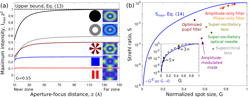
Figure 4: (a) Intensity bounds for various aperture shapes (normalized to far-zone bound, Eq. (13)). The bounds, scaled by $z^{2}$ for aperture–focus distance $z$, are largest in the far zone, where the optimal field profiles (inset images) are highly dependent on the aperture shape. Equation (13) is the general bound of the circumscribing circle for each shape, represented in the dashed line. (b) Maximum Strehl ratio (Eq. (14)) compared to previous designs, including amplitude Gundu et al. (2005)/phase de Juana et al. (2003)-only pupil filters, optimized pupil filters Kosmeier et al. (2011), a super-oscillatory lens Rogers et al. (2012), a super-oscillatory optical needle Rogers et al. (2013), a supercritical lens Qin et al. (2017), and an amplitude-modulated mask Dong et al. (2017). Inset: Our bound (blue), despite allowing for arbitrary diffractive optical elements, is smaller than the bound of Ref. Sales and Morris (1997) (black dashed), which requires rotation symmetry in the scalar and weak-scattering limit.

Figure 4(a) plots the intensity bound, Eq. (9), for a variety of exit-aperture shapes and from the near zone to the far zone, with a generic spot size $G=0.55$. The bound is scaled by $z^{2}$, the square of the aperture–focus distance, to account for the quadratic power decay. In each case the far-zone bound is larger than that of the near zone or mid zone, suggesting that the far-zone bounds of Eq. (13) and Eq. (14) may be global bounds at any distance. For each case, the maximum intensity is bounded above by the bound for the circumscribing circle (solid black line), while the optimal field profiles are highly dependent on the aperture shapes (inset images).

Figure 4(b) plots the far-zone bound $S_{\max}$ as a function of spot size $G$ (blue curve), and compares various theoretical results from the literature de Juana et al. (2003); Gundu et al. (2005); Kosmeier et al. (2011); Rogers et al. (2012, 2013); Qin et al. (2017); Dong et al. (2017). (Many of the references include experimental results; for fair comparison and to exclude experimental errors, we use either their simulated $G$ and $S$ values, or reconstruct them with our own simulations as detailed in the SM.) For relatively large spot sizes ($G>0.7$), theoretical proposals for amplitude Gundu et al. (2005) or phase de Juana et al. (2003) filters can closely approach the limits, though embedded in the proposals is a weak-scattering assumption that may be difficult to achieve in practice. (The key reason they fall short of the bound is that they do not allow for multiple scattering to redistribute energy in the exit plane.) For small spot sizes, on the other hand, the maximum Strehl ratio decreases rapidly. A Taylor expansion of Eq. (14) reveals the asymptotic bound (SM),

$$S_{\rm max}=\zeta_{0}^{4}/192,\quad\zeta_{0}\ll 1,$$ (15)

which represents a severe restriction—halving the spot size costs a sixteenfold decrease in maximum focal intensity. This fundamental limit suggests that extremely small spot sizes are impractical, from both power-consumption and fabrication-tolerance perspectives. The quartic dependence is independent of dimensionality (in the SM we show that the same dependence arises for a focal sphere, as well as for focal points in 2D problems) and can be explained generally: for small enough spot sizes, the zero-contour field will always have a maximum at the origin and thus all odd powers in a Taylor expansion around the origin must be zero. The first non-constant field dependence in the expansion is quadratic, and since the overlap quantities in the intensity bound are themselves quadratic in the field, the general intensity dependence on spot size always results in an $\sim\zeta_{0}^{4}$ scaling law. (While this is reminiscent of the quartic dependence between the transmission through a subwavelength hole in a conducting screen and the hole size Bethe (1944), we show in the SM that their physical origins are unrelated.)

Perhaps the most important region of the figure is for intermediate values of spot size ($0.1\lesssim G\lesssim 0.7$), where it is possible to meaningfully shrink the spot size below the diffraction limit without an overwhelming sacrifice of intensity. This is the region that recent designs Kosmeier et al. (2011); Rogers et al. (2012, 2013); Qin et al. (2017); Dong et al. (2017) have targeted (especially $0.5<G<0.7$) with a variety of approaches, including super-oscillatory lenses/needles and optimized pupil filters. Yet as seen in Fig. 4(a), these designs mostly fall dramatically short of the bounds. The best result by this metric is the “optimized pupil filter” of Kosmeier et al. (2011), whose quadratic-programming approach comes within a factor of 5 of the bound, and demonstrates the utility of computational-design approaches for maximum intensity. The other designs fall short of the bounds by factors of 100-1000X or more, offering the possibility for significant improvement by judicious design of the diffractive optical element(s).

The inset of Fig. 4(b) compares our analytical bound of Eq. (14) to the computational bounds of Sales and Morris (1997), which used special-function expansions to identify upper limits to intensity as a function of spot size for scalar, rotation-symmetric waves in the weak-scattering limit. Perhaps surprisingly, despite allowing for far more general optical setups and for vector waves without any symmetry or weak-scattering assumptions, our bounds are 3-5X smaller than those of Sales and Morris (1997). (An analytical bound coinciding with Eq. (14) has been derived in Liu et al. (2002), albeit assuming rotational symmetry in a scalar approximation and without the other general results herein.) Note conversely, however, that our approach is also prescriptive, in the sense that it identifies the exact field profiles that can reach our bounds.

We can also characterize the effective currents on the aperture that achieve the bound in Eq. (14). For spot sizes close to the diffraction limit ($G=1$), the currents are maximally concentrated around the aperture rim and decreases towards the center, where the amplitude is close to zero. This is because small, localized spots require large transverse wavevector components, which originate from the currents around the rim. As spot size decreases, those edge currents are partially redistributed to the center, to create the interference effects giving rise to sub-diffraction-limited spots.

Given the feasibility of achieving sub-diffraction-limited waves, it is important to contextualize the recent work of Ref. (Miller, 2019, Sec. 5.5), which uses a singular-value-decomposition approach to identify possible field patterns that can be generated. In that work, it is shown that sub-diffraction-limited Gaussian field profiles require exponentially large input powers, and suggested that therefore sub-diffraction-limited focusing is essentially impossible. The key distinction our work makes is loosening the requirement for a Gaussian field profile, instead imposing only spot-size constraints on the field without reference to any desired profile. This more general problem has feasible, sub-diffraction-limited solutions whose input powers scale only polynomially with spot size.

As discussed above, our bounds, both in the general case of Eq. (6) and in the optical-beam case of Eq. (13), are tight in the sense that they are achievable by fields that are solutions of Maxwell’s equations, given by $\psi=\bm{\Gamma}\xi_{\rm opt}$. Yet as shown in Fig. 4, theoretical designs for sub-diffraction-limited beams have fallen far short of the bounds. A natural question, then, is whether realistic material patterning and designs can generate the requisite fields to achieve the bounds?

III Inverse-designed metasurfaces

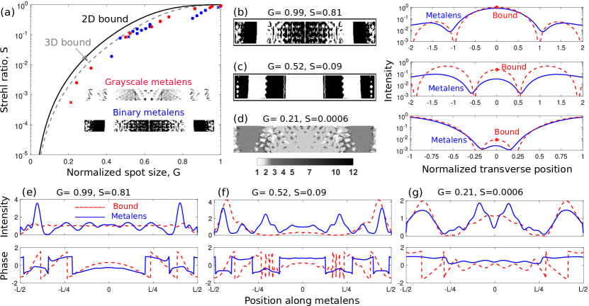
Figure 5: (a) Inverse-designed metasurfaces, with grayscale (gradient-index, red circles) and binary (blue circles) material distributions, approach the 2D bounds (black line) of Eq. (16) for a variety of spot sizes. The similar 3D bound of Eq. (14) is included for comparison with Fig. 4. Three specific designs, highlighted with an “$\times$” marker in (a), are shown in (b,c,d), along with their intensity profiles on the focal plane (blue line) and those achieving the 2D bounds (red dashed line), normalized relative to the diffraction-limited intensity for each case. (e,f,g) Field intensity (normalized to the incident intensity) and phase profiles near the exit surface ($2\lambda$ from metasurface) for the corresponding designs in (b,c,d), compared to those achieving the 2D bounds. The focal distance is set to $50\lambda$, and the metasurfaces have widths $L=23\lambda$ for $G=0.99,0.52$ and $L=10\lambda$ for $G=0.21$.

We use “inverse design” to discover refractive-index profiles that can approach the concentration bounds. Inverse design Jensen and Sigmund (2011); Miller (2012); Bendsoe and Sigmund (2013); Molesky et al. (2018) is a large-scale computational-optimization technique, mathematically equivalent to backpropagation in neural networks Rumelhart et al. (1986); LeCun et al. (1989); Werbos (1994), that enables rapid computation of sensitivities with respect to arbitrarily many structural/material degrees of freedom. Given such sensitivities, standard optimization techniques Nocedal and Wright (2006) such as gradient descent (employed here) can be used to discover locally optimal structures, often exhibiting orders-of-magnitude better performance Lalau-Keraly et al. (2013); Ganapati et al. (2014) than structures with few parameters designed by hand or brute force.

For some target wavelength $\lambda$, we consider metasurfaces with thicknesses of $1.9\lambda$ and widths (diameters) ranging from $10\lambda$ to $23\lambda$, equivalent to films with thicknesses on the order of 1${\mu}$m and widths in the dozens of microns for visible-frequency light. We consider two-dimensional scattering (i.e. metasurfaces that are translation-invariant along one dimension), to reduce the computational cost and demonstrate the design principle. Dimensionality has only a small effect on the bounds; in the SM, we show that the 2D equivalent of Eq. (14) is

$$S_{\rm max}^{2D}=1-\frac{4}{\zeta_{0}}\frac{\sin^{2}(\zeta_{0})}{\sin(2\zeta_{0})+2\zeta_{0}}.$$ (16)

For the design variables, we allow the permittivity at every point on the metasurface to vary (i.e., “topology optimization” Jensen and Sigmund (2011); Bendsoe and Sigmund (2013)), and we generate two types of designs (depicted in Fig. 5): binary metasurfaces, in which the permittivity must take one of two values (chosen here as 1 and 12), and grayscale metasurfaces, in which the permittivity can vary smoothly between two values as in gradient-index optics Marchand (1978).

The optical figure of merit $F$ that we use to discover optimal design is not exactly the zero-point intensity of Eq. (4), as the zero-field constraint is difficult to implement numerically. Instead, for a desired spot size $G$, we subtract a constant $\alpha$ times the field intensity at the points $\pm G$ away from the origin:

$$F=|\psi(0)|^{2}-\alpha\left(\left|\psi(-G)\right|^{2}+\left|\psi(G)\right|^{2}\right).$$ (17)

This is a penalty method Bertsekas (2014) that can enforce arbitrarily small field intensities (with sufficiently accurate simulations) by increasing the constant $\alpha$ over the course of the optimization. We take the electric field polarized out of the plane, such that $\psi$ can be simplified to a scalar field solution of the Helmholtz equation, which we solve by the finite-difference time-domain (FDTD) method  Taflove et al. (2013); Oskooi et al. (2010). Adjoint-based sensitivities are computed for every structural iteration via two computations: the “direct” fields propagating through the metasurface, and “adjoint” fields that emanate from the maximum-intensity and zero-field locations, with phases and amplitudes of the exciting currents determined by the derivatives of Eq. (17) with respect to the field.

Figure 5 depicts the results of many inverse-designed metasurfaces. Figure 5(a) compares the bound of Eq. (16) (black; the nearly identical 3D bound is in grey) to the computed Strehl ratio of unique optimal designs at spot sizes ranging from 0.21 to 1; strikingly, the designed metalenses closely approach the bound for all spot sizes, with the best designs achieving 90% of the maximum possible intensity. In Fig. 5(b,c,d) three specific designs are shown alongside the resulting field profiles in their focal planes (we provide a full list of permittivity values at each grid point of these three metasurface designs in the SM). The intensity does not perfectly reach zero but is forced to be significantly smaller than the peak intensity through the penalty constant $\alpha$ in Eq. (17). The field intensities and phases on the exit surface (2$\lambda$ from metasurface) are shown in Fig. 5(e,f,g) corresponding to the three designs. Fig. 5(e) shows good qualitative agreement with the ideal field profiles achieving the 2D bounds, and even for smaller spot sizes the designed metasurfaces achieve the intensity redistributions—exhibited by local intensities larger than one—required to approach the bounds (Fig. 5(f,g)). It is difficult to explain exactly how the computationally designed metasurface patterns achieve nearly optimal focusing; for spot sizes close to 1, the variations in material density suggest an effective gradient-index-like profile that offers lens-like phase variations across the device width, though the scattering effects of the front and rear surfaces renders such explanations necessarily incomplete. The depicted design with $G=0.21$ exhibits to our knowledge the smallest spot size of any theoretical proposal to date.

IV Alternative spot-size metrics

To this point, we have considered the problem of maximizing field intensity subject to a spot size defined by the field equaling zero around a prescribed contour. Of course, this is not the only metric one might consider. In this section, we consider two alternative definitions of spot size which do not require the field to go to zero anywhere, and which enforce “concentration” through other characteristics of an optical beam. The two properties that we consider are the full-width at half-maximum (FWHM) of the beam, a commonly used metric for experimental measurements Huang et al. (2007a); Kitamura et al. (2010); Rogers et al. (2012, 2013); Qin et al. (2015), and the local wavenumber (as measured by the spatial variations in the field), whose maximization was an impetus for early work in super-oscillations Berry (1994a, b); Kempf and Ferreira (2004); Berry and Popescu (2006); Aharonov et al. (2011); Lindberg (2012). We show that using these constraints, the corresponding field-concentration problems can be formulated as nonconvex, quadratically constrained quadratic programs (QCQPs) whose global bounds can be found computationally in reasonable (polynomial) time. For the canonical far-zone scenario considered in Sec. II, we compare the optimal beams for the three metrics: a zero-field contour, a FWHM spot-size, and a minimum local wavevector, and we find that the beams are nearly identical. These numerical experiments suggest that the intensities and optimal-beam profiles found by our analytical bounds for the zero-field-contour metric may describe optimal beams across a wide swath of possible “concentration” metrics.

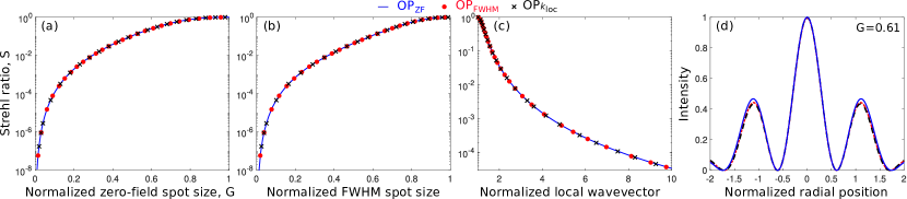
Figure 6: Optimal beam characteristics for three concentration metrics: $OP_{\textrm{ZF}}$ (Eq. (4), blue lines), $OP_{\textrm{FWHM}}$ (Eq. (18), red circles) and $OP_{\textrm{kloc}}$ (Eq. (19), black crosses) refer to the optimization problems with constraints on the zero-field spot size $G$, FWHM spot size, and the local wavevector respectively. (a,b,c) Bounds plotted against spot-size radius, FWHM, and local wavevector at the focal point, $k_{\textrm{loc}}(\mathbf{x}=0)$, respectively (all normalized to those of a diffraction-limited beam). (d) Optimal beam profiles with zero-field spot size $G=0.61$ for the three different optimization problems, showing nearly identical beam profiles, especially around the central peak.

For each of the alternative metrics we consider, we retain the objective of maximizing intensity at the origin, and replace the zero-field-contour constraint with a constraint on another property. As a first alternative, we impose a constraint that requires the average field intensity to fall to its FWHM value within a prescribed, sub-diffraction-limited contour $\mathcal{C}$. The average field value around the contour is given by $\frac{1}{\left|\mathcal{C}\right|}\int_{\mathcal{C}}\,|\psi(\mathbf{x})|^{2}\,{\rm d}\mathbf{x}=\xi^{\dagger}\left[\left(1/|\mathcal{C}|\right)\int_{\mathcal{C}}\bm{\Gamma}^{\dagger}\bm{\Gamma}\right]\xi$, where $\left|\mathcal{C}\right|$ denotes the perimeter of contour $\mathcal{C}$. We denote this optimization problem “(OP_FWHM),” which is written:

$${\rm(OP_{FWHM})}$$ (18)

$$\underset{\xi}{\text{maximize}} I(\mathbf{x}=0)=\xi^{\dagger}\bm{\Gamma}_{0}^{\dagger}\bm{\Gamma}_{0}\xi$$

subject to $$\xi^{\dagger}\left[\frac{1}{|\mathcal{C}|}\int_{\mathcal{C}}\bm{\Gamma}^{\dagger}\bm{\Gamma}\right]\xi\leq\frac{1}{2}\xi^{\dagger}\bm{\Gamma}_{0}^{\dagger}\bm{\Gamma}_{0}\xi$$

$$\xi^{\dagger}\xi\leq 1,$$

where the objective represents the intensity at the origin, the first constraint enforces the FWHM to occur within the contour $\mathcal{C}$, and the second constraint is the power normalization.

As a second alternative, we consider one of the early definitions of “super-oscillations:” a signal comprising spatial frequencies up to some maximum $k$ can have a “local,” position-dependent wavenumber $k_{\rm loc}(\mathbf{x})$, as measured by spatial variations in the field, that is in fact larger than $k$ by an arbitrary extent Berry and Popescu (2006). To define $k_{\rm loc}$, one could use a gradient-based expression like $-i\nabla$, yet the resulting operator would not be Hermitian, limiting its viability. Instead, we use the negative Laplacian, a positive-definite real-symmetric operator (for fields that decay sufficiently fast), normalized by the field intensity at the origin: $k_{\rm loc}(\mathbf{x})=\sqrt{-\nabla^{2}|\psi(\mathbf{x})|^{2}/|\psi(0)|^{2}}$. For a plane wave $e^{i\bm{\mathbf{k}}\cdot\mathbf{x}}$, the local wavenumber equals that of the plane wave, i.e., $k_{\rm loc}(\mathbf{x})=|\bm{\mathbf{k}}|$. Thus, an alternative way to define a tightly confined beam would be to require the local wavenumber at the origin to be at least as large as some $k_{\rm loc,min}$ that is much larger than the free-space wavenumber $\omega/c$, i.e. $k_{\rm loc,min}\gg\omega/c$. In this optimization-problem formulation, denoted by “(OP_kloc),” we now use the constraint $k_{\rm loc}^{2}(\mathbf{x}=0)\geq k_{\rm loc,min}^{2}$:

$${\rm(OP_{kloc})}$$ (19)

$$\underset{\xi}{\text{maximize}} I(\mathbf{x}=0)=\xi^{\dagger}\bm{\Gamma}_{0}^{\dagger}\bm{\Gamma}_{0}\xi$$

subject to $$\xi^{\dagger}\left[-\nabla^{2}\left(\bm{\Gamma}^{\dagger}\bm{\Gamma}\right)\big{\rvert}_{\mathbf{x}=0}\right]\xi\geq k^{2}_{\textrm{loc,min}}\xi^{\dagger}\bm{\Gamma}_{0}^{\dagger}\bm{\Gamma}_{0}\xi$$

$$\xi^{\dagger}\xi\leq 1,$$

where in the $k_{\rm loc}$ constraint we have moved the field normalization $|\psi(0)|^{2}$ to the right-hand side, such that the quadratic nature of the problem is readily apparent.

The two alternative optimization problems, (OP_FWHM) and (OP_kloc), both comprise nonconvex quadratic objectives subject to two quadratic constraints (one convex and one nonconvex in each case). It is not possible (to our knowledge) to identify analytical bounds for such objectives. However, one can use semidefinite relaxation (SDR), a now-standard technique Luo et al. (2010) in optimization theory, to “relax” the problem from a quadratic one for variables $\xi$ of size $N$ to a linear one in a much larger space of dimension $N^{2}$, for which interior-point methods can find global optima Nocedal and Wright (2006). Typically, such relaxations lead to bounds that may be “loose,” i.e. unattainable, but it is known in QCQP theory Huang and Zhang (2007) that for complex-variable quadratic problems with three or fewer constraints, SDR bounds are “tight,” i.e. attainable (due to a duality gap that is strictly zero). Thus, we can use SDR to compute exact bounds and field profiles for problems (OP_FWHM) and (OP_kloc).

We can briefly summarize the application of SDR to problems (OP_FWHM) and (OP_kloc). Each problem is of the form

$$\underset{\xi}{\text{maximize}} \xi^{\dagger}\bm{\mathbf{A}}\xi$$ (20)

subject to $$\xi^{\dagger}\bm{\mathbf{B}}\xi\leq 0$$

$$\xi^{\dagger}\xi\leq 1.$$

The first idea in SDR is to rewrite terms of the form $\xi^{\dagger}\bm{\mathbf{A}}\xi$ as $\operatorname{Tr}\left(\bm{\mathbf{A}}\xi\xi^{\dagger}\right)$, and then define the positive semidefinite, rank-one matrix $\bm{\mathbf{X}}$ by $\bm{\mathbf{X}}=\xi\xi^{\dagger}$, such that $\xi^{\dagger}\bm{\mathbf{A}}\xi=\operatorname{Tr}\left(\bm{\mathbf{A}}\bm{\mathbf{X}}\right)$. Then Eq. (20) is equivalent to

$$\underset{\xi}{\text{maximize}} \operatorname{Tr}\left(\bm{\mathbf{A}}\bm{\mathbf{X}}\right)$$ (21)

subject to $$\operatorname{Tr}\left(\bm{\mathbf{B}}\bm{\mathbf{X}}\right)\leq 0$$

$$\operatorname{Tr}\left(\bm{\mathbf{X}}\right)\leq 1$$

$$\bm{\mathbf{X}}\succeq 0,\quad\operatorname{rank}(\bm{\mathbf{X}})=1.$$

The objective and constraints in Eq. (21) are all linear in $\bm{\mathbf{X}}$ except for the constraint $\operatorname{rank}(\bm{\mathbf{X}})=1$. The “relaxation” of SDR denotes dropping this rank-one constraint, leaving a linear program whose solution represents an upper bound (for our maximization problem) for the original quadratic program. By the QCQP theory for fewer than four constraints, as discussed above, this bound is tight.

Figure 6 compares the analytical bounds of the zero-field optimization problem, (OP_ZF), to the computational SDR bounds for the alternative optimization problems, (OP_FWHM) and (OP_kloc). Each bound is computed for many sub-diffraction-limited values of a different parameter: (OP_ZF) with respect to the zero-field spot size, (OP_FWHM) with respect to the FWHM spot size, and (OP_kloc) with respect to the local wavevector (all normalized relative to the respective values for a diffraction-limited beam, cf. SM). There is no simple mapping between these three parameters, but we can measure those parameters for the optimal beams of each of the three optimization problems, and Fig. 6(a–c) shows the results. One can see that the optimal beams for the three different problems exhibit nearly identical parameters. This suggests that the beams themselves might be very similar, and this is confirmed in Fig. 6(d), which shows the optimal beams for the three metrics that all exhibit a normalized zero-field spot size $G=0.61$, and from which it is clear that the beams themselves are nearly identical, especially near the origin and up to the first zero. In this region, the relative difference between each pair of the beams is less than 1%. This striking similarity suggests two conclusions: first, the optimal beam profiles are “robust,” in the sense that changing the concentration definition may result in nearly equivalent beams, and second, that our analytical bounds may describe even the optimal concentration that is possible as defined by a wide variety of metrics. (Of course, one can concoct metrics that must have different bounds; e.g., if the objective is maximum intensity subject to small intensity within some “window” that represents a field of view, then certainly the corresponding bounds must depend on the size of the window. However, our analytical expressions would still almost certainly represent upper bounds, since they would represent the limit of a very small window.)

V Summary and Extensions

We have established bounds on the maximal concentration of free-space vector electromagnetic waves. We derive bounds for any desired zero-field contour, either incorporating an aperture as in Eqs. (6,9,14) or dependent only on a modal basis, as in Eqs. (6,12). By a suitable transformation of the light-concentration problem, we obtain analytic bounds in multiple regimes (small spot sizes, far zone, etc.), providing insight into the ideal excitation field as well as revealing a dimension-independent quartic spot-size scaling law. Using inverse design, we have theoretically proposed optimal metasurface designs approaching these bounds. We have also demonstrated that the ideal beam profiles under alternative spot-size metrics are nearly identical to those for the zero-field-contour metric in the far zone.

Looking forward, there are a number of related questions and application areas where this approach can be applied. One may further explore other field-concentration metrics. For example, we can ask if it is feasible to specify certain target Maxwell fields on a contour. We show in the SM that the problem of maximizing focal intensity given a target field profile on some contour can be reduced to a complex-variable QCQP with one constraint. As explained in the previous section, such problems can be solved in polynomial time by SDR. In this way, we obtain exact, global bounds and physically attainable fields. One may also be interested in metrics other than focal-point intensity. One common metric, a minimal-energy metric for a fixed focal-point intensity Levi (1965); Ferreira and Kempf (2006), in fact is equivalent to focal-point maximization metric under constraints of fixed energy, as can be shown by comparing the Lagrangian functions of each. Other metrics, potentially focusing on minimizing energy within a specific region (e.g., the field of view), can be seamlessly incorporated into the approach developed here.

We have considered the medium through which light propagates to be free space (or any homogeneous material, which simply modifies the speed of light in the medium), but our results in fact apply directly to any inhomogeneous background by using the corresponding Green’s function in Eq. (6). For near-field imaging with the image plane near some scattering medium, our approach can identify the optimal resolution. It can also potentially be applied to random media Mosk et al. (2012), where the Green’s function can be appropriately modified through ensemble averaging, to potentially identify optimal concentration within complex disordered media.

One can also explore bounds to other related phenomena such as superdirectivity Schelkunoff (1943); Hansen (1981)—directivity greater than that obtained with the same antenna configuration uniformly excited. Just as achieving sub-diffraction-limited beams relies on a delicate interference of propagating waves, superdirectivity requires structured antenna arrays with finely tuned excitation amplitudes. Superdirective antennas suffer from diminished efficiency and large sidelobe energies Hansen (1981), and the bound techniques developed herein may provide deeper insight or generalized bounds for such phenomena.

Finally, we can expect that the bounds here can be used as a family of potential point-spread functions across imaging applications. Various emerging techniques at the intersection of quantum optics, metrology, and parameter estimation theory Tsang et al. (2016); Zhou and Jiang (2019) suggest the possibility for imaging with resolution improvements beyond the classical Rayleigh limit and Airy disk. A tandem of the sub-diffraction-limited point-spread functions provided here with quantum measurement theory may yield even further improvements.

VI Acknowledgments

We thank Michael Fiddy and Lawrence Domash for helpful conversations. H. S., H. C., and O. D. M. were partially supported by DARPA and Triton Systems under award number 140D6318C0011, and were partially supported by the Air Force Office of Scientific Research under award number FA9550-17-1-0093.

References

- McCutchen (1967) C. W. McCutchen, Superresolution in Microscopy and the Abbe Resolution Limit, Journal of the Optical Society of America 57, 1190 (1967).
- Stelzer (2002) E. H. K. Stelzer, Beyond the diffraction limit?, Nature 417, 806 (2002).
- Zheludev (2008) N. I. Zheludev, What diffraction limit?, Nature Materials 7, 420 (2008).
- Gustafsson (2005) M. G. L. Gustafsson, Nonlinear structured-illumination microscopy: Wide-field fluorescence imaging with theoretically unlimited resolution, Proceedings of the National Academy of Sciences 102, 13081 (2005).
- Betzig et al. (2006) E. Betzig, G. H. Patterson, R. Sougrat, O. W. Lindwasser, S. Olenych, J. S. Bonifacino, M. W. Davidson, J. Lippincott-Schwartz, and H. F. Hess, Imaging Intracellular Fluorescent Proteins at Nanometer Resolution, Science 313, 1642 (2006).
- Rust et al. (2006) M. J. Rust, M. Bates, and X. Zhuang, Sub-diffraction-limit imaging by stochastic optical reconstruction microscopy (STORM), Nature Methods 3, 793 (2006).
- Hell (2007) S. W. Hell, Far-field optical nanoscopy, Science 316, 1153 (2007).
- Huang et al. (2008) B. Huang, W. Wang, M. Bates, and X. Zhuang, Three-Dimensional Super-Resolution Imaging by Stochastic Optical Reconstruction Microscopy, Science 319, 810 (2008).
- Lipson and Kurman (2013) H. Lipson and M. Kurman, Fabricated: The new world of 3D printing (John Wiley & Sons, 2013).
- Chia and Wu (2015) H. N. Chia and B. M. Wu, Recent advances in 3D printing of biomaterials, Journal of Biological Engineering 9, 4 (2015).
- Huang and Zheludev (2009) F. M. Huang and N. I. Zheludev, Super-resolution without evanescent waves, Nano Letters 9, 1249 (2009).
- Rogers et al. (2012) E. T. Rogers, J. Lindberg, T. Roy, S. Savo, J. E. Chad, M. R. Dennis, and N. I. Zheludev, A super-oscillatory lens optical microscope for subwavelength imaging, Nature Materials 11, 432 (2012).
- Strehl (1902) K. Strehl, Über luftschlieren und zonenfehler, Zeitschrift für Instrumentenkunde 22, 213 (1902).
- Born and Wolf (2013) M. Born and E. Wolf, Principles of optics: electromagnetic theory of propagation, interference and diffraction of light (Elsevier, 2013).
- Bertsekas (2016) D. P. Bertsekas, Nonlinear programming, 3rd ed. (Athena Scientific, Belmont, MA, 2016).
- Slepian (1961) D. Slepian, Prolate Spheroidal Wave Functions, Fourier Analysis and Uncertainty — I, Bell System Technical Journal 40, 43 (1961).
- Landau and Pollak (1961) H. J. Landau and H. O. Pollak, Prolate Spheroidal Wave Functions, Fourier Analysis and Uncertainty — II, Bell System Technical Journal 40, 65 (1961).
- Ferreira and Kempf (2006) P. J. Ferreira and A. Kempf, Superoscillations: Faster than the Nyquist rate, IEEE Transactions on Signal Processing 54, 3732 (2006).
- Jensen and Sigmund (2011) J. S. Jensen and O. Sigmund, Topology optimization for nano-photonics, Laser and Photonics Reviews 5, 308 (2011).
- Miller (2012) O. D. Miller, Photonic Design: From Fundamental Solar Cell Physics to Computational Inverse Design, Ph.D. thesis, University of California, Berkeley (2012).
- Bendsoe and Sigmund (2013) M. P. Bendsoe and O. Sigmund, Topology optimization: theory, methods, and applications (Springer Science & Business Media, 2013).
- Molesky et al. (2018) S. Molesky, Z. Lin, A. Y. Piggott, W. Jin, J. Vucković, and A. W. Rodriguez, Inverse design in nanophotonics, Nature Photonics 12, 659 (2018).
- Kawata et al. (1989) H. Kawata, J. M. Carter, A. Yen, and H. I. Smith, Optical projection lithography using lenses with numerical apertures greater than unity, Microelectronic Engineering 9, 31 (1989).
- Ito and Okazaki (2000) T. Ito and S. Okazaki, Pushing the limits of lithography, Nature 406, 1027 (2000).
- Odom et al. (2002) T. W. Odom, V. R. Thalladi, J. C. Love, and G. M. Whitesides, Generation of 30-50 nm structures using easily fabricated, composite PDMS masks, Journal of the American Chemical Society 124, 12112 (2002).
- Rugar (1984) D. Rugar, Resolution beyond the diffraction limit in the acoustic microscope: A nonlinear effect, Journal of Applied Physics 56, 1338 (1984).
- Indebetouw et al. (2007) G. Indebetouw, Y. Tada, J. Rosen, and G. Brooker, Scanning holographic microscopy with resolution exceeding the Rayleigh limit of the objective by superposition of off-axis holograms, Applied Optics 46, 993 (2007).
- Kumar et al. (2012) K. Kumar, H. Duan, R. S. Hegde, S. C. Koh, J. N. Wei, and J. K. Yang, Printing colour at the optical diffraction limit, Nature Nanotechnology 7, 557 (2012).
- Collier (2013) R. Collier, Optical holography (Elsevier, 2013).
- Moskovits (1985) M. Moskovits, Surface-enhanced spectroscopy, Reviews of Modern Physics 57, 783 (1985).
- Nie and Emory (1997) S. Nie and S. R. Emory, Probing single molecules and single nanoparticles by surface-enhanced Raman scattering, Science 275, 1102 (1997).
- Kneipp et al. (1997) K. Kneipp, Y. Wang, H. Kneipp, L. T. Perelman, I. Itzkan, R. R. Dasari, and M. S. Feld, Single Molecule Detection Using Surface-Enhanced Raman Scattering (SERS), Physical Review Letters 78, 1667 (1997).
- Ebbesen et al. (1998) T. W. Ebbesen, H. J. Lezec, H. F. Ghaemi, T. Thio, and P. A. Wolff, Extraordinary optical transmission through sub-wavelength hole arrays, Nature 391, 667 (1998).
- Martín-Moreno et al. (2001) L. Martín-Moreno, F. J. García-Vidal, H. J. Lezec, K. M. Pellerin, T. Thio, J. B. Pendry, and T. W. Ebbesen, Theory of extraordinary optical transmission through subwavelength hole arrays, Physical Review Letters 86, 1114 (2001).
- Genet and Ebbesen (2007) C. Genet and T. W. Ebbesen, Light in tiny holes, Nature 445, 39 (2007).
- Fang et al. (2005) N. Fang, H. Lee, C. Sun, and X. Zhang, Sub–Diffraction-Limited Optical Imaging with a Silver Superlens, Science 308, 534 (2005).
- Kostelak et al. (1991) R. L. Kostelak, J. S. Weiner, E. Betzig, T. D. Harris, and J. K. Trautman, Breaking the Diffraction Barrier: Optical Microscopy on a Nanometric Scale, Science 251, 1468 (1991).
- Merlin (2007) R. Merlin, Radiationless Electromagnetic Interference: Evanescent-Field Lenses and Perfect Focusing, Science 317, 927 (2007).
- Zhang and Liu (2008) X. Zhang and Z. Liu, Superlenses to overcome the diffraction limit, Nature Materials 7, 435 (2008).
- Ma et al. (2018) G. Ma, X. Fan, F. Ma, J. De Rosny, P. Sheng, and M. Fink, Towards anti-causal Green’s function for three-dimensional sub-diffraction focusing, Nature Physics 14, 608 (2018).
- Toraldo di Francia (1952) G. Toraldo di Francia, Super-gain antennas and optical resolving power, Il Nuovo Cimento 9, 426 (1952).
- Schelkunoff (1943) S. A. Schelkunoff, A mathematical theory of linear arrays, The Bell System Technical Journal 22, 80 (1943).
- Berry (1994a) M. Berry, Faster than Fourier in quantum coherence and reality Celebration of the 60th Birthday of Yakir Aharonov ed JS Anandan and JL Safko (1994a).
- Berry (1994b) M. V. Berry, Evanescent and real waves in quantum billiards and Gaussian beams, Journal of Physics A: Mathematical and General 27, L391 (1994b).
- Berry and Popescu (2006) M. V. Berry and S. Popescu, Evolution of quantum superoscillations and optical superresolution without evanescent waves, Journal of Physics A: Mathematical and General 39, 6965 (2006).
- Lindberg (2012) J. Lindberg, Mathematical concepts of optical superresolution, Journal of Optics 14, 083001 (2012).
- Kempf and Ferreira (2004) A. Kempf and P. J. Ferreira, Unusual properties of superoscillating particles, Journal of Physics A: Mathematical and General 37, 12067 (2004).
- Aharonov et al. (2011) Y. Aharonov, F. Colombo, I. Sabadini, D. C. Struppa, and J. Tollaksen, Some mathematical properties of superoscillations, Journal of Physics A: Mathematical and Theoretical 44, 365304 (2011).
- Wong and Eleftheriades (2010) A. M. H. Wong and G. V. Eleftheriades, Adaptation of Schelkunoff’s Superdirective Antenna Theory for the Realization of Superoscillatory Antenna Arrays, IEEE Antennas and Wireless Propagation Letters 9, 315 (2010).
- Chremmos and Fikioris (2015) I. Chremmos and G. Fikioris, Superoscillations with arbitrary polynomial shape, Journal of Physics A: Mathematical and Theoretical 48, 265204 (2015).
- Smith and Gbur (2016) M. K. Smith and G. J. Gbur, Construction of arbitrary vortex and superoscillatory fields, Optics Letters 41, 4979 (2016).
- Bassett (1986) I. M. Bassett, Limit to concentration by focusing, Optica Acta 33, 279 (1986).
- Sheppard and Larkin (1994) C. J. R. Sheppard and K. G. Larkin, Optimal concentration of electromagnetic radiation, Journal of Modern Optics 41, 1495 (1994).
- Sales and Morris (1997) T. R. M. Sales and G. M. Morris, Fundamental limits of optical superresolution, Optics Letters 22, 582 (1997).
- Liu et al. (2002) H. Liu, Y. Yan, Q. Tan, and G. Jin, Theories for the design of diffractive superresolution elements and limits of optical superresolution, Journal of the Optical Society of America A 19, 2185 (2002).
- Rogers et al. (2018) K. S. Rogers, K. N. Bourdakos, G. H. Yuan, S. Mahajan, and E. T. F. Rogers, Optimising superoscillatory spots for far-field super-resolution imaging, Optics Express 26, 8095 (2018).
- Miller (2019) D. A. B. Miller, Waves, modes, communications, and optics: a tutorial, Advances in Optics and Photonics 11, 679 (2019).
- Pfeiffer and Grbic (2013) C. Pfeiffer and A. Grbic, Metamaterial Huygens’ Surfaces: Tailoring Wave Fronts with Reflectionless Sheets, Physical Review Letters 110, 197401 (2013).
- Huang et al. (2007a) F. M. Huang, N. Zheludev, Y. Chen, and F. Javier Garcia De Abajo, Focusing of light by a nanohole array, Applied Physics Letters 90, 091119 (2007a).
- Huang et al. (2007b) F. M. Huang, Y. Chen, F. J. Garcia De Abajo, and N. I. Zheludev, Optical super-resolution through super-oscillations, Journal of Optics A: Pure and Applied Optics 9, S285 (2007b).
- Dennis et al. (2008) M. R. Dennis, A. C. Hamilton, and J. Courtial, Superoscillation in speckle patterns, 33, 2976 (2008).
- Wang et al. (2009) X. Wang, J. Fu, X. Liu, and L.-M. Tong, Subwavelength focusing by a micro/nanofiber array, Journal of the Optical Society of America A 26, 1827 (2009).
- Kitamura et al. (2010) K. Kitamura, K. Sakai, and S. Noda, Sub-wavelength focal spot with long depth of focus generated by radially polarized, narrow-width annular beam, Optics Express 18, 4518 (2010).
- Rogers et al. (2013) E. T. Rogers, S. Savo, J. Lindberg, T. Roy, M. R. Dennis, and N. I. Zheludev, Super-oscillatory optical needle, Applied Physics Letters 102, 031108 (2013).
- Huang et al. (2013) L. Huang, X. Chen, H. Mühlenbernd, H. Zhang, S. Chen, B. Bai, Q. Tan, G. Jin, K. W. Cheah, C. W. Qiu, J. Li, T. Zentgraf, and S. Zhang, Three-dimensional optical holography using a plasmonic metasurface, Nature Communications 4, 2808 (2013).
- Huang et al. (2014) K. Huang, H. Ye, J. Teng, S. P. Yeo, B. Luk’yanchuk, and C. W. Qiu, Optimization-free superoscillatory lens using phase and amplitude masks, Laser and Photonics Reviews 8, 152 (2014).
- Qin et al. (2015) F. Qin, K. Huang, J. Wu, J. Jiao, X. Luo, C. Qiu, and M. Hong, Shaping a subwavelength needle with ultra-long focal length by focusing azimuthally polarized light, Scientific Reports 5, 9977 (2015).
- Wong and Eleftheriades (2015) A. M. Wong and G. V. Eleftheriades, Superoscillations without Sidebands: Power-Efficient Sub-Diffraction Imaging with Propagating Waves, Scientific Reports 5, 8449 (2015).
- Wong and Eleftheriades (2017) A. M. Wong and G. V. Eleftheriades, Broadband superoscillation brings a wave into perfect three-dimensional focus, Physical Review B 95, 075148 (2017).
- Kildishev et al. (2013) A. V. Kildishev, A. Boltasseva, and V. M. Shalaev, Planar photonics with metasurfaces, Science 339, 1232009 (2013).
- Yu and Capasso (2014) N. Yu and F. Capasso, Flat optics with designer metasurfaces, Nature Materials 13, 139 (2014).
- Khorasaninejad et al. (2016) M. Khorasaninejad, W. T. Chen, R. C. Devlin, J. Oh, A. Y. Zhu, and F. Capasso, Metalenses at visible wavelengths: Diffraction-limited focusing and subwavelength resolution imaging, Science 352, 1190 (2016).
- Li et al. (2018) A. Li, S. Singh, and D. Sievenpiper, Metasurfaces and their applications, Nanophotonics 7, 989 (2018).
- Serrels et al. (2008) K. A. Serrels, E. Ramsay, R. J. Warburton, and D. T. Reid, Nanoscale optical microscopy in the vectorial focusing regime, Nature Photonics 2, 311 (2008).
- Jabbour and Kuebler (2008) T. G. Jabbour and S. M. Kuebler, Vectorial beam shaping, Optics Express 16, 7203 (2008).
- Bauer et al. (2014) T. Bauer, S. Orlov, U. Peschel, P. Banzer, and G. Leuchs, Nanointerferometric amplitude and phase reconstruction of tightly focused vector beams, Nature Photonics 8, 23 (2014).
- Lin et al. (2019) Z. Lin, V. Liu, R. Pestourie, and S. G. Johnson, Topology optimization of freeform large-area metasurfaces, Optics Express 27, 15765 (2019).
- Chung and Miller (2019) H. Chung and O. D. Miller, High-NA, Achromatic, Visible-Frequency Metalenses by Inverse Design, arXiv preprint arXiv:1905.09213 (2019).
- Kong (1975) J. A. Kong, Theory of electromagnetic waves (Wiley-Interscience, New York, 1975).
- Levy et al. (2007) U. Levy, M. Abashin, K. Ikeda, A. Krishnamoorthy, J. Cunningham, and Y. Fainman, Inhomogenous dielectric metamaterials with space-variant polarizability, Physical Review Letters 98, 243901 (2007).
- Wei et al. (2013) Z. Wei, Y. Long, Z. Gong, H. Li, X. Su, and Y. Cao, Highly efficient beam steering with a transparent metasurface, Optics Express 21, 10739 (2013).
- Keren-Zur et al. (2016) S. Keren-Zur, O. Avayu, L. Michaeli, and T. Ellenbogen, Nonlinear Beam Shaping with Plasmonic Metasurfaces, ACS Photonics 3, 117 (2016).
- Weiner (2000) A. M. Weiner, Femtosecond pulse shaping using spatial light modulators, Review of Scientific Instruments 71, 1929 (2000).
- Chattrapiban et al. (2003) N. Chattrapiban, E. A. Rogers, D. Cofield, W. T. Hill, III, and R. Roy, Generation of nondiffracting Bessel beams by use of a spatial light modulator, Optics Letters 28, 2183 (2003).
- Guo et al. (2007) C.-S. Guo, X.-L. Wang, W.-J. Ni, H.-T. Wang, and J. Ding, Generation of arbitrary vector beams with a spatial light modulator and a common path interferometric arrangement, Optics Letters 32, 3549 (2007).
- Zhu and Wang (2014) L. Zhu and J. Wang, Arbitrary manipulation of spatial amplitude and phase using phase-only spatial light modulators, Scientific Reports 4, 7441 (2014).
- Lodahl et al. (2004) P. Lodahl, A. F. Van Driel, I. S. Nikolaev, A. Irman, K. Overgaag, D. Vanmaekelbergh, and W. L. Vos, Controlling the dynamics of spontaneous emission from quantum dots by photonic crystals, Nature 430, 654 (2004).
- Ringler et al. (2008) M. Ringler, A. Schwemer, M. Wunderlich, A. Nichtl, K. Kürzinger, T. A. Klar, and J. Feldmann, Shaping Emission Spectra of Fluorescent Molecules with Single Plasmonic Nanoresonators, Physical Review Letters 100, 203002 (2008).
- Bleuse et al. (2011) J. Bleuse, J. Claudon, M. Creasey, N. S. Malik, J.-M. Gérard, I. Maksymov, J.-P. Hugonin, and P. Lalanne, Inhibition, Enhancement, and Control of Spontaneous Emission in Photonic Nanowires, Physical Review Letters 106, 103601 (2011).
- Epstein and Eleftheriades (2016) A. Epstein and G. V. Eleftheriades, Huygens’ metasurfaces via the equivalence principle: design and applications, Journal of the Optical Society of America B 33, A31 (2016).
- Ra’di et al. (2017) Y. Ra’di, D. L. Sounas, and A. Alù, Metagratings: Beyond the Limits of Graded Metasurfaces for Wave Front Control, Physical Review Letters 119, 067404 (2017).
- Gustafsson and Nordebo (2013) M. Gustafsson and S. Nordebo, Optimal antenna currents for Q, superdirectivity, and radiation patterns using convex optimization, IEEE Transactions on Antennas and Propagation 61, 1109 (2013).
- Shi et al. (2017) S. Shi, L. Wang, and B. L. G. Jonsson, Antenna Current Optimization and Realizations for Far-Field Pattern Shaping, arXiv preprint arXiv:1711.09709v2 (2017).
- Chew (1995) W. C. Chew, Waves and fields in inhomogeneous media (IEEE press, 1995).
- Jin (2011) J.-M. Jin, Theory and computation of electromagnetic fields (John Wiley & Sons, 2011).
- Boyd and Vandenberghe (2004) S. Boyd and L. Vandenberghe, Convex optimization (Cambridge university press, 2004).
- Horn and Johnson (2013) R. A. Horn and C. R. Johnson, Matrix analysis, 2nd ed. (Cambridge university press, 2013).
- Trefethen and Bau III (1997) L. N. Trefethen and D. Bau III, Numerical linear algebra (SIAM, 1997).
- Boyd (2001) J. P. Boyd, Chebyshev and Fourier spectral methods, 2nd ed. (Dover, New York, 2001).
- Levy et al. (2016) U. Levy, S. Derevyanko, and Y. Silberberg, Light Modes of Free Space, Progress in Optics 61, 237 (2016).
- Mazilu et al. (2011) M. Mazilu, J. Baumgartl, S. Kosmeier, and K. Dholakia, Optical Eigenmodes; exploiting the quadratic nature of the light-matter interaction, Optics Express 19, 933 (2011).
- Kosmeier et al. (2011) S. Kosmeier, M. Mazilu, J. Baumgartl, and K. Dholakia, Enhanced two-point resolution using optical eigenmode optimized pupil functions, Journal of Optics 13, 105707 (2011).
- Levi (1965) L. Levi, Fitting a bandlimited signal to given points, IEEE Transactions on Information Theory 11, 372 (1965).
- Slepian (1978) D. Slepian, Prolate Spheroidal Wave Functions, Fourier Analysis, and Uncertainty—V: The Discrete Case, Bell System Technical Journal 57, 1371 (1978).
- Gundu et al. (2005) P. N. Gundu, E. Hack, and P. Rastogi, ’Apodized superresolution’ - Concept and simulations, Optics Communications 249, 101 (2005).
- de Juana et al. (2003) D. M. de Juana, J. E. Oti, V. F. Canales, and M. P. Cagigal, Design of superresolving continuous phase filters, Optics Letters 28, 607 (2003).
- Qin et al. (2017) F. Qin, K. Huang, J. Wu, J. Teng, C. W. Qiu, and M. Hong, A Supercritical Lens Optical Label-Free Microscopy: Sub-Diffraction Resolution and Ultra-Long Working Distance, Advanced Materials 29, 1602721 (2017).
- Dong et al. (2017) X. H. Dong, A. M. H. Wong, M. Kim, and G. V. Eleftheriades, Superresolution far-field imaging of complex objects using reduced superoscillating ripples, Optica 4, 1126 (2017).
- Bethe (1944) H. A. Bethe, Theory of diffraction by small holes, Physical Review 66, 163 (1944).
- Rumelhart et al. (1986) D. E. Rumelhart, G. E. Hinton, and R. J. Williams, Learning representations by back-propagating errors, Nature 323, 533 (1986).
- LeCun et al. (1989) Y. LeCun, B. Boser, J. S. Denker, D. Henderson, R. E. Howard, W. Hubbard, and L. D. Jackel, Backpropagation Applied to Handwritten Zip Code Recognition, Neural Computation 1, 541 (1989).
- Werbos (1994) P. J. Werbos, The Roots of Backpropagation (John Wiley & Sons, Inc., 1994).
- Nocedal and Wright (2006) J. Nocedal and S. J. Wright, Numerical Optimization, 2nd ed. (Springer, New York, NY, 2006).
- Lalau-Keraly et al. (2013) C. M. Lalau-Keraly, S. Bhargava, O. D. Miller, and E. Yablonovitch, Adjoint shape optimization applied to electromagnetic design, Optics Express 21, 21693 (2013).
- Ganapati et al. (2014) V. Ganapati, O. D. Miller, and E. Yablonovitch, Light trapping textures designed by electromagnetic optimization for subwavelength thick solar cells, IEEE Journal of Photovoltaics 4, 175 (2014).
- Marchand (1978) E. Marchand, Gradient index optics (Academic, New York, 1978).
- Bertsekas (2014) D. P. Bertsekas, Constrained optimization and Lagrange multiplier methods (Academic press, 2014).
- Taflove et al. (2013) A. Taflove, A. Oskooi, and S. G. Johnson, Advances in FDTD computational electrodynamics: photonics and nanotechnology (Artech house, 2013).
- Oskooi et al. (2010) A. F. Oskooi, D. Roundy, M. Ibanescu, P. Bermel, J. D. Joannopoulos, and S. G. Johnson, Meep: A flexible free-software package for electromagnetic simulations by the FDTD method, Computer Physics Communications 181, 687 (2010).
- Luo et al. (2010) Z. Q. Luo, W. K. Ma, A. So, Y. Ye, and S. Zhang, Semidefinite relaxation of quadratic optimization problems, IEEE Signal Processing Magazine 27, 20 (2010).
- Huang and Zhang (2007) Y. Huang and S. Zhang, Complex matrix decomposition and quadratic programming, Mathematics of Operations Research 32, 758 (2007).
- Mosk et al. (2012) A. P. Mosk, A. Lagendijk, G. Lerosey, and M. Fink, Controlling waves in space and time for imaging and focusing in complex media, Nature Photonics 6, 283 (2012).
- Hansen (1981) R. Hansen, Fundamental limitations in antennas, Proceedings of the IEEE 69, 170 (1981).
- Tsang et al. (2016) M. Tsang, R. Nair, and X. M. Lu, Quantum theory of superresolution for two incoherent optical point sources, Physical Review X 6, 031033 (2016).
- Zhou and Jiang (2019) S. Zhou and L. Jiang, Modern description of Rayleigh’s criterion, Physical Review A 99, 013808 (2019).