Measuring the growth of structure by matching dark matter haloes to galaxies with VIPERS and SDSS

Abstract

We test the history of structure formation from redshift 1 to today by matching galaxies from the VIMOS Public Extragalactic Redshift Survey (VIPERS) and Sloan Digital Sky Survey (SDSS) with dark matter haloes in the MultiDark, Small MultiDark Planck (SMDPL), N-body simulation. We first show that the standard subhalo abundance matching (SHAM) recipe implemented with MultiDark fits the clustering of galaxies well both at redshift 0 for SDSS and at redshift 1 for VIPERS. This is an important validation of the SHAM model at high redshift. We then remap the simulation time steps to test alternative growth histories and infer the growth index $\gamma=0.6\pm 0.3$. This analysis demonstrates the power of using N-body simulations to forward model galaxy surveys for cosmological inference. The data products and code necessary to reproduce the results of this analysis are available online (https://github.com/darklight-cosmology/vipers-sham).

1 Introduction

The growth of structure over cosmic time is a fundamental observable that informs us about the expansion history and the physics of gravitational instability, both of which are key ingredients for interpreting cosmic acceleration (e.g. Huterer et al., 2015). Surveys that map the distribution of galaxies out to high redshift provide important measurements of the statistics of the matter field and its evolution. In the standard paradigm galaxies form inside massive dark matter clumps, and these clumps build up hierarchically (White & Frenk, 1991). The formation of dark matter structures and their spatial statistics have been well investigated analytically and in $N$-body simulations (e.g. Bardeen et al., 1986; Springel et al., 2005).

However, the connection between the galaxies detected in surveys and the underlying matter distribution is complex (Baugh, 2013; Wechsler & Tinker, 2018). Observations show that the two-point clustering statistics depend strongly on the luminosity, colour, morphology and other physical properties of the galaxy sample (Davis & Geller, 1976; Giovanelli et al., 1986; Guzzo et al., 1997; Norberg et al., 2002; Zehavi et al., 2005; Pollo et al., 2006; Marulli et al., 2013; Cappi et al., 2015; Di Porto et al., 2016) since these properties are tied to the density environments the galaxies are found in (Blanton & Berlind, 2007; Davidzon et al., 2016; Cucciati et al., 2017). These dependencies are encoded in the galaxy bias $b_{g}$ that relates the two-point clustering statistics of the galaxies to that of the underlying matter on large scales: $\xi_{g}(r,z)=b_{g}(z)^{2}\xi(r,z)$ (Kaiser, 1984). It is the usual practice to parametrize the bias function and marginalise over these parameters in a cosmological analysis since they depend on the galaxy sample and the peculiarities of the survey selection function (Rota et al., 2017; Alam et al., 2017). Other approaches have been developed to infer the biasing function using statistics of the galaxy distribution. Di Porto et al. (2016) constrain the bias by matching the galaxy density distribution measured in a galaxy survey with the distribution of dark matter in an $N$-body simulation assuming a one-to-one correspondence. We will follow a similar approach in this analysis using dark matter haloes.

The process of matching the dark matter haloes in a simulation to the distribution of galaxies selected by luminosity or stellar mass in a survey known as sub-halo abundance matching (SHAM) provides a simple yet accurate prediction of galaxy bias (Vale & Ostriker, 2004; Conroy et al., 2006; Behroozi et al., 2010; Moster et al., 2010; Trujillo-Gomez et al., 2011). The method requires an $N$-body simulation with sufficient resolution to identify and follow the substructure within dark matter haloes (Guo & White, 2014). Reddick et al. (2013) demonstrate that a single halo property is sufficient to assign galaxies and that the implicit choice of this property primarily affects the clustering on small scales below 1$h^{-1}{\rm Mpc}$. Stochasticity or scatter in the relationship between the halo mass and the galaxy luminosity has been shown to be less important when the galaxy sample is sufficiently deep such that it is complete down to the characteristic flattening of the luminosity function (or stellar mass function) (Conroy et al., 2006; Reddick et al., 2013).

At low redshift, spectroscopic surveys including the Two-degree Field Galaxy Redshift Survey (2dFGRS), the Sloan Digital Sky Survey (SDSS) Main galaxy sample and the Galaxy And Mass Assembly (GAMA) survey have appropriately broad and deep selection functions. At higher redshift, the VIMOS Public Extragalactic Redshift Survey (VIPERS, Guzzo et al., 2014; Scodeggio et al., 2018) is unique with a cosmologically representative volume.

The accuracy of SHAM to model galaxy clustering over cosmic time was first demonstrated by Conroy et al. (2006) who compiled galaxy clustering measurements to $z\sim 5$. Conroy et al. (2006) developed a SHAM model to assign galaxy luminosities to haloes using the equivalent of the halo property $V_{peak}$ that we define below. No additional free parameters such as stochasticity or scatter in the assignment were used. The success of Conroy et al. (2006) has motivated the development of the SHAM model that we adopt to describe the clustering of galaxies in SDSS and VIPERS.

The application of SHAM without free parameters is attractive for making cosmological predictions. For example, He et al. (2018) extended SHAM to modified gravity models and tested the validity of these models against the standard $\Lambda$ cold dark matter scenario using galaxy clustering statistics. To extend this technique more generally to constrain cosmological parameters requires a large number of simulations that span a range of cosmological models (Harker et al., 2007). However, a practical shortcut can be taken to avoid this computational expense. It has been shown that a simulation run in one model can be made to quantitatively look like a simulation run in a different model by re-scaling the time and spatial dimensions to match the expansion and growth histories (Angulo & White, 2010; Mead & Peacock, 2014a, b; Mead et al., 2015; Zennaro et al., 2019). This approach was implemented in a cosmological analysis pipeline by Simha & Cole (2013).

We apply the re-scaling algorithm here in a simplified context in which we vary only the growth history quantified by $\sigma_{8}$, the variance of the linear matter field on 8$h^{-1}{\rm Mpc}$ scales. In practice, modifying the evolution of $\sigma_{8}(z)$ in a simulation requires only re-labeling the redshift of the outputs. Using the MultiDark $N$-body simulation (Klypin et al., 2016), we employ a parameter-free SHAM model to predict the galaxy correlation function and directly constrain $\sigma_{8}(z)$ using measurements at redshift $z<0.106$ in SDSS and at redshift $0.5<z<1$ in VIPERS. Harker et al. (2007) made a similar analysis on SDSS that employed semi-analytic models for galaxy formation to predict the amplitude of galaxy clustering. Simha & Cole (2013) carried out a full cosmological analysis using SDSS making use of re-scaled simulations and SHAM. We present the preliminary application of these techniques to higher redshift.

The growth history $\sigma_{8}(z)$ may be parametrized by the growth index $\gamma$ as (Wang & Steinhardt, 1998)

$$\sigma_{8}(z)=\sigma_{8}(0)\exp\left[-\int_{0}^{z}\Omega_{m}(z^{\prime})^{\gamma}d\ln(1+z^{\prime})\right].$$ (1)

The growth index in the standard model is $\gamma=0.55$. Other parametrizations have been proposed more recently (e.g. Silvestri et al., 2013); however, the use of the growth index neatly separates the dependence on the expansion history given by $\Omega_{m}(z)$ from modifications to the gravity model (Linder, 2005; Guzzo et al., 2008; Moresco & Marulli, 2017).

In this paper we first present a validation of the SHAM model over the redshift range $0<z<1$ using well-characterised galaxy samples from SDSS and VIPERS (Sec. 2, 3). To give an additional test of the underlying assumptions we select galaxies by luminosity and stellar mass with matching number densities so that they share the same SHAM prediction. We study systematic errors arising from incompleteness and scatter in Sec. 4. After demonstrating the robustness of the SHAM model, we apply the re-scaling algorithm to the MultiDark simulation and infer the cosmological growth of structure (Sec. 5). Section 6 concludes with a discussion of the results.

2 Galaxy redshift surveys

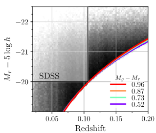
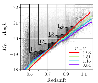
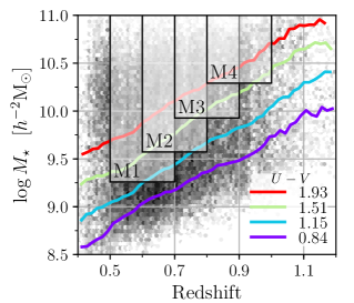
Figure 1: The SDSS and VIPERS samples used in this study. Left: The selection of the SDSS sample on the absolute magnitude in the $r$ band, $M_{r}$. Middle: the selection of the VIPERS luminosity samples on $M_{B}$ with an evolution trend. Right: the selection of the VIPERS stellar mass samples. In each panel the 90% completeness limits are indicated by the lines as a function of the galaxy colour from blue to red (the colour is $M_{g}-M_{r}$ for SDSS and $U-V$ for VIPERS).

Figure 2: The distribution of the VIPERS sample as a function of $U-V$ colour, absolute magnitude $M_{B}$ and stellar mass for the four redshift bins. The contours contain 25, 50 and 90% of the sample. The horizontal and vertical dotted lines mark the stellar mass and absolute magnitude thresholds respectively of the subsamples used in the analysis. The solid and dashed curves indicate the 90 and 50% completeness limits in stellar mass and absolute magnitude as a function of colour. The red sequence is above the stellar mass completeness limit in each redshift bin.

Sample	Redshift	Mean z	Threshold	Count	Volume	Density
					$10^{6}h^{-3}{\rm Mpc}^{3}$	$10^{-3}h^{3}{\rm Mpc}^{-3}$
SDSS	$0.020<z<0.106$	0.063	$M_{r}<-20.0$	117959	21.90	5.85
L1	$0.5<z<0.7$	0.61	$M_{B}<-19.3+(0.7-z)$	23352	4.93	11.8
M1	$0.5<z<0.7$	0.61	$\log M_{\star}>9.26h^{-2}{\rm M_{\odot}}$	22508	4.93	11.8
L2	$0.6<z<0.8$	0.70	$M_{B}<-19.8+(0.8-z)$	20579	5.98	8.57
M2	$0.6<z<0.8$	0.70	$\log M_{\star}>9.57h^{-2}{\rm M_{\odot}}$	19577	5.98	8.57
L3	$0.7<z<0.9$	0.80	$M_{B}<-20.3+(0.9-z)$	13046	6.96	4.79
M3	$0.7<z<0.9$	0.80	$\log M_{\star}>9.93h^{-2}{\rm M_{\odot}}$	12270	6.96	4.79
L4	$0.8<z<1.0$	0.90	$M_{B}<-20.8+(1.0-z)$	6305	7.86	2.13
M4	$0.8<z<1.0$	0.89	$\log M_{\star}>10.29h^{-2}{\rm M_{\odot}}$	5881	7.86	2.13

Table 1: The galaxy samples used in this study. The number density is weighted to correct for survey incompleteness.

2.1 SDSS Main Galaxy Sample at z < 0.1

The Sloan Digital Sky Survey (SDSS, York et al. 2000) main galaxy sample (MGS, Strauss et al. 2002) provides a flux-limited census of galaxies in the low-redshift universe. In this paper, we use the SDSS MGS Data Release 7 (DR7, Abazajian et al. 2009), which includes spectroscopy and photometry for 499,546 galaxies with Petrosian extinction-corrected r-band magnitude $r<17.77$ at $z<0.22$, over 7300 square degrees.

We obtain the MGS data from the NYU Value Added Galaxy Catalogs (NYU-VAGC, Blanton et al. 2005), which provide K-corrections, absolute magnitudes, completeness weights and the survey mask. We use the DR7 LSS catalog, which employs a more restrictive r-band cut at $r<17.6$ in order to ensure a homogeneous selection across the SDSS footprint. The absolute magnitudes in the ugriz bands included in the LSS catalog are K-corrected to $z_{0}=0.1$ using kcorrect (Blanton et al., 2003). By blue-shifting the rest-frame to $z=0.1$, the effect of the correction is minimised.

The NYU-VAGC provides all the elements needed to measure the SDSS correlation function, including survey mask, randoms, and galaxy weights. Following the procedure described in Favole et al. (2017), the NYU-VAGC randoms are corrected for the variation of completeness across the SDSS footprint. This correction is performed by down-sampling the random catalogue with equal surface density in a random fashion using the completeness as a probability function (see Section 3 in Favole et al. 2017 for more details).

We apply two different galaxy weights to correct for angular incompleteness. The fiber collision weight, w_fc, accounts for the fact that fibers on the same tile cannot be placed closer than 55 arcsec. These weights correspond to the total number of neighbours within a 55-arcsec radius of each MGS galaxy for which redshift was not measured due to fiber collisions (i.e., w${}_{fc}\geq$ 0). The second weight, w_c, accounts for the redshift measurement success rate in the mask sector where each galaxy lies, so that w${}_{c}\leq$ 1. The average completeness of the MGS is $\sim$80$\%$ (see Montero-Dorta & Prada 2009). In the computation of the correlation function, each galaxy is counted as $(1+w_{fc})w_{c}$ and each random as $w_{c}$ since we previously diluted the random catalogue using the $w_{c}$ measurement completeness.

We select a single sample in the redshift range $0.02<z<0.106$ by imposing an r-band absolute-magnitude threshold ${}^{0.1}{\rm M}_{r}<-20.0$. The uncertainty on the SDSS clustering measurement is estimated from the covariance matrix of 200 jackknife resamplings with constant galaxy number density (Favole et al., 2016b).

2.2 VIPERS at 0.5 < z < 1

The VIMOS Public Extragalactic Redshift Survey (VIPERS Guzzo et al., 2014; Scodeggio et al., 2018) provides high-fidelity maps of the galaxy field at higher redshift. The survey measured 90 000 galaxies with moderate resolution spectroscopy using the Visible Multi-Object Spectrograph (VIMOS) at VLT. Targets were selected to a limiting magnitude of $i_{AB}=22.5$ in 24 square degrees of the CFHTLS Wide imaging survey. The low redshift limit was imposed by a pre-selection based upon color which effectively removed foreground galaxies while providing a robust flux-limited selection at $z>0.5$.

The completeness of the VIPERS sample with respect to the parent flux-limited sample is well-characterised in terms of the target sampling rate (TSR) and spectroscopic redshift measurement success rate (SSR) (Scodeggio et al., 2018). Additionally, close pairs of galaxies could not be targeted due to slit placement constraints leading to a drop in the correlation function at very small scales $<1h^{-1}{\rm Mpc}$. We correct for this effect by up-weighting pairs according to their angular separation when computing the correlation function (see Pezzotta et al., 2017).

The VIPERS sample has photometric measurements from the UV to infrared which have been used to infer the luminosity and stellar masses of the galaxies (Davidzon et al., 2013; Fritz et al., 2014; Davidzon et al., 2016; Moutard et al., 2016). The absolute magnitudes are presented assuming a standard flat cosmological model with $\Omega_{m}=0.3$ and $h=1$, but note that we compute the the number density of the samples in the MultiDark cosmology for the SHAM analysis. The distribution of the rest-frame magnitude $M_{B}$ is shown in Fig. 1.

For the analysis we select four samples in overlapping bins of redshift with thresholds in $M_{B}$. These samples are labelled L1, L2, L3 and L4 and listed in Table 1. We impose an evolving luminosity limit to account for the luminosity trend for a passively evolving stellar population as applied in previous VIPERS analyses (e.g. Marulli et al., 2013). The selection threshold in a redshift bin $z_{0}<z<z_{1}$ is specified as: $M_{limit}=M_{z_{1}}+(z_{1}-z)$. We also construct matching samples selected by stellar mass that have the same number density. These samples are labelled M1, M2, M3 and M4. The number density is computed as the weighted sum to correct for TSR and SSR. The completeness limits as a function of luminosity, stellar mass and colour are shown in Fig. 2.

We make use of the VIPERS mock galaxy catalogues to estimate the covariance of the correlation function measurements. These catalogues were built from the Big Multidark $N$-body simulation (Klypin et al., 2016). Galaxies were simulated using the halo occupation distribution (HOD) technique calibrated to reproduce the number density and projected correlation function of VIPERS galaxies in bins of luminosity and redshift (de la Torre et al., 2013, 2017). In total, 153 independent realisations of the full VIPERS survey are available.

For each VIPERS sample we select a comparable sample from the mock catalogues by setting a threshold in luminosity that gives the same number density. We confirm that the projected correlation function of these mock samples approximately matches the amplitude of the VIPERS measurements.

3 Matching with dark matter haloes

We use the MultiDark $N$-body numerical simulation (Klypin et al., 2016) to model the distribution and evolution of dark matter haloes. We choose the Small MultiDark Planck (SMDPL) box, of side length $400h^{-1}\rm{Mpc}$, containing a total of 3840³ particles. The simulation assumes a $\Lambda$CDM cosmology (Planck Collaboration et al., 2014), with parameters $h=0.677$, $\Omega_{m}=0.307$, $\Omega_{\Lambda}=0.693$, $n_{s}=0.96$ and $\sigma_{8}=0.823$. Dark-matter haloes (including subhaloes) were identified using the ROCKSTAR code (Behroozi et al., 2013).

We make the connection between galaxies measured in VIPERS or SDSS and haloes from the SMDPL snapshots with sub-halo abundance matching (SHAM, Vale & Ostriker 2004). The link to the simulated haloes is made using the peak maximum circular velocity of the particles in the halo over its formation history ($V_{peak}$). The $V_{peak}$ property characterizes the halo mass before disruption processes occur and it has been demonstrated that this is important for modelling the distribution of satellite galaxies. Velocity is used instead of virial mass because it is more robustly defined in simulations. For further details we refer the reader to Conroy et al. 2006; Trujillo-Gomez et al. 2011; Reddick et al. 2013; Campbell et al. 2018.

We select galaxies based upon a stellar mass (or luminosity) threshold. Then, within a single simulation snapshot we select haloes by setting a threshold in $V_{peak}$ that results in an equal number density. These haloes become the mock galaxies for the analysis. In Sec. 4 we test the impact of scatter or stochasticity in the relationship between the halo and galaxy properties. However, our main results are derived without scatter and in this case the SHAM model is determined solely by the densities of the samples listed in Table 1.

Fig. 3 shows the distributions of haloes at $z=0$ and $z=1$ as a function of virial mass $M_{vir}$ and $V_{peak}$. Two $V_{peak}$ threshold selections are indicated that give number densities $10^{-2}$ and $10^{-3}h^{3}{\rm Mpc}^{-3}$. The median halo mass of the higher density selection is $M_{vir}\sim 7.5\times 10^{11}h^{-1}{\rm M_{\odot}}$ at $z=1$ which corresponds to 7500 simulation particles and guarantees that the haloes selected for the SHAM analysis are robustly defined (Guo & White, 2014).

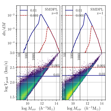
Figure 3: The distribution of $V_{peak}$ and $M_{vir}$ halo properties in SMDPL at $z=0$ (left panels) and $z=1$ (right panels). The horizontal solid and dashed lines in the bottom panels indicate thresholds in $V_{peak}$ that give number densities of $10^{-2}$ and $10^{-3}h^{3}{\rm Mpc}^{-3}$. The $M_{vir}$ distributions after applying these selections are shown in the top panels (solid and dashed histograms). The vertical dotted lines indicate the virial mass corresponding to 10, 100 and 1000 simulation particles.

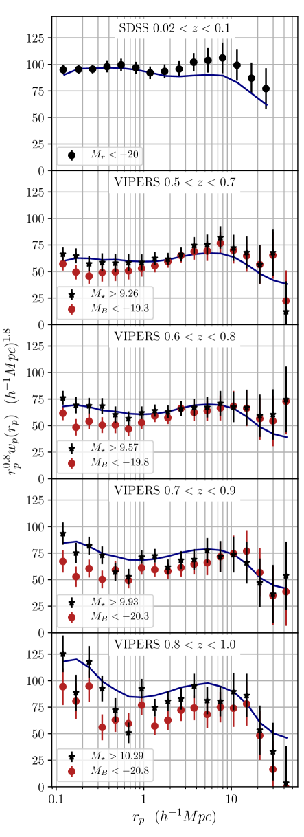
Figure 4: The projected correlation function measured in SDSS (top panel) and VIPERS (bottom four panels) in luminosity and stellar mass selected samples. The matched samples have the same number density and thus share the same SHAM model (solid curve).

The clustering amplitude of the galaxy field can be inferred from measurements of the projected correlation function without being strongly impacted by the redshift-space distortion signal caused by peculiar velocities (Davis & Peebles, 1983). The projected correlation function $w_{p}$ depends on the perpendicular separation $r_{p}$ and is computed by integrating along the line-of-sight ($\pi$ direction):

$$w_{p}(r_{p})=2\int_{0}^{\pi_{max}}\xi_{g}\left(r_{p},\pi^{\prime}\right)d\pi^{\prime}.$$ (2)

We set the integration limit to $\pi_{max}=50h^{-1}{\rm Mpc}$.

We compute the redshift-space correlation function $\xi(r_{p},\pi)$ for the galaxy surveys using the Landy-Szalay estimator (Landy & Szalay, 1993). We employ two correlation function code implementations, that of Favole et al. (2017) and CUTE (Alonso, 2012). The correlation functions of the MultiDark SHAM samples are computed in the plane-parallel approximation taking advantage of the periodic boundaries of the cubic simulation box. The residual redshift-space distortion signal in the projected correlation function is present both in the galaxy and halo measurements, so we do not make any additional corrections.

We compute the projected correlation functions for the SHAM models at the redshifts of the MultiDark snapshots, $w_{p}^{halo}(r_{p},z|n)$, where $n$ is the number density of the galaxy sample. To compute the model between the simulation snapshots at an arbitrary redshift we build a linear interpolation function that is based on the principal component decomposition using the first two eigenvectors.

Fig. 4 shows the measured correlation function for each galaxy sample and the corresponding SHAM model at the sample redshift. There is good agreement between the SHAM model and the SDSS measurements. This confirms previous studies that developed and tested the SHAM model on the SDSS galaxy correlation function (e.g. Reddick et al., 2013).

We find that the VIPERS luminosity selected samples have a clustering amplitude that is systematically lower than the stellar mass selected samples. This discrepancy is more significant at smaller scales $r_{p}<1h^{-1}Mpc$ and in the highest redshift bin. In each redshift bin the luminosity and stellar mass selected samples were constructed to share the same SHAM prediction, thus we find that the SHAM model better reproduces the clustering of the stellar mass-selected sample.

The systematic difference in clustering amplitude between the luminosity and stellar mass-selected samples is not unexpected since hydrodynamic simulations have demonstrated that galaxy stellar mass is a better indicator for the host halo mass (Chaves-Montero et al., 2016). We would expect the choice to be less important when selecting galaxies based upon the rest-frame luminosity in a redder band that is more tightly correlated to the stellar mass (Bell & de Jong, 2001). This can explain the agreement with SHAM seen in SDSS projected correlation functions for both $M_{r}$ selected and mass selected samples (Reddick et al., 2013). On the other hand, the bluer rest-frame band used in VIPERS (that is closest to the observed $i$ selection band) is more sensitive to recent star formation activity and hence is less informative of the total mass of the galaxy. The consequence is that in VIPERS, the correlation function of galaxies selected in $M_{B}$ is lower than for those selected by stellar mass. This effect should become more important at higher redshift as the rest frame for a fixed bandpass shifts to the blue and star formation activity becomes more prevalent (Haines et al., 2017).

4 Systematics

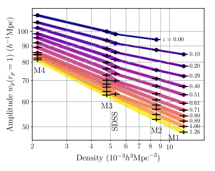
Figure 5: The correlation function amplitude at $r=1h^{-1}{\rm Mpc}$ versus galaxy number density of all SHAM samples used in our analysis. The error bars correspond to 5% variation in number density, which is representative of the VIPERS sample variance. In order to change the amplitude by 10% requires a change of number density of 50% at z=0 and 30% at z=1.

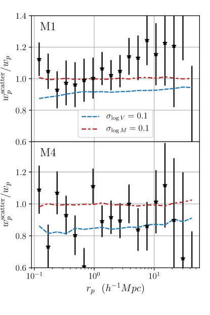
Figure 6: The relative change in the correlation function after introducing scatter in the SHAM procedure is shown for two mass-selected samples in VIPERS M1 $0.5<z<0.7$ (top) and M4 $0.8<z<1.0$ (bottom). A Gaussian scatter of 0.1 dex was applied to $M_{\star}$ (dash-dotted curve) or $V_{peak}$ (dashed curve).

We have found that the SHAM model can predict the galaxy clustering signal to redshift 1; however, it is important to make note of the assumptions that have been made and consider how extensions to the SHAM recipe would affect our results. On the observational side, uncertainty in the number density due to sample variance or incompleteness propagates to the SHAM model as a systematic error. Fig. 5 summarises the SHAM models that we constructed for this work and demonstrates the power-law relationship between the clustering amplitude at $r=1h^{-1}{\rm Mpc}$ and number density. The horizontal error bars on this plot indicate 5% variations in number density which is representative of the sample variance in the VIPERS samples. The vertical error bar propagates this error to the amplitude of the correlation function and is at the percent level. In order to change the amplitude of the correlation function by 10% requires varying the number density by 50% at $z=0$ and 30% at $z=1$. These conclusions follow from the SHAM model that imposes that the clustering amplitude is determined only by stellar mass (or other halo mass proxy). This is not precisely true since galaxy colour correlates with the density of the environment at fixed stellar mass (e.g. Davidzon et al., 2016).

We also see from Fig. 5 that the SHAM prediction becomes less sensitive to redshift at lower number density. Therefore, to improve the constraining power requires higher density samples which at high redshift becomes observationally challenging.

The SHAM procedure can be extended to improve the precision of the predictions. Scatter can be introduced to account for the fact that galaxies of a specific stellar mass are associated with a greater variety of halo properties than the SHAM dictates. This may be due to stochastic processes or error in the host halo assignment due to missing physical ingredients. Investigations with hydrodynamic simulations indicate that the relationship between galaxy stellar mass and halo $V_{peak}$ is approximately 0.1 dex (Chaves-Montero et al., 2016).

Fig. 6 shows the effect of scatter following two approaches. First, we consider scatter applied to the stellar mass (Behroozi et al. 2010, see also Trujillo-Gomez et al. (2011) who apply scatter to luminosity). From the observational perspective, this scatter cannot be too large otherwise the intrinsic (deconvolved) stellar mass function would be inconsistent with observations. A large scatter also requires extrapolating the stellar mass function to low masses below observational limits. We thus test scatter in stellar mass of 0.1 dex. We find that scatter of $\sigma_{\log M}=0.1$ dex has no effect on the measured correlation function at the percent level for the number densities of the VIPERS samples. This is due to the fact that the stellar mass function is flattening at the selection threshold (Reddick et al., 2013).

Next we consider a dispersion in $V_{peak}$. This implies that $V_{peak}$ is not a perfect proxy for galaxy assignment. The advantage of applying scatter to $V_{peak}$ is that a large scatter may be introduced without modifying the stellar mass function of galaxies. We find that the scatter of $\sigma_{\log V}=0.1$ dex does modify the amplitude of the correlation function by 10 to 20% in the VIPERS samples. The scatter can improve the match of the VIPERS data at high redshift but is not required given the statistical error. However, scatter at the same level applied at lower redshift is ruled out. The introduction of free parameters to account for redshift-dependent scatter would greatly limit the cosmological interpretation.

5 Growth of structure

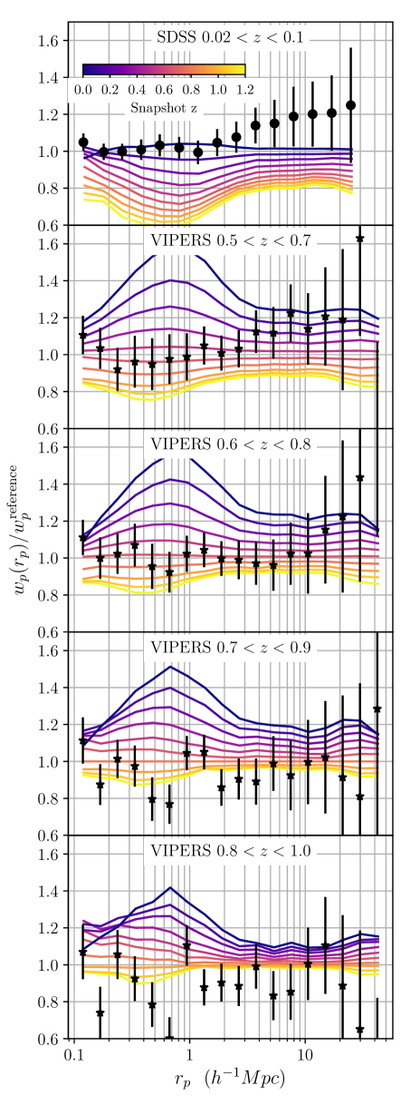
Figure 7: The SHAM model projected correlation functions computed over a range of simulation redshifts $0<z<1.2$. In each panel the correlation function has been divided by the SHAM model at the sample redshift. The data points indicate the SDSS sample (top panel) and VIPERS stellar mass selected samples (bottom four panels).

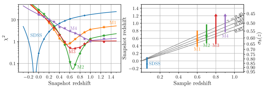
Figure 8: Left: the $\chi^{2}$ statistics for each galaxy sample (SDSS, M1, M2, M3, M4) as a function of redshift. The markers indicate the SHAM models computed from the simulation snapshots while the curves were derived by linear interpolation of the models. Negative snapshot redshifts (scale factor $>1$) corresponds to running the simulation into the future. Right: The best-fitting SHAM model as a function of its simulation snapshot is plotted for each galaxy sample shown on the left. The right-most scale indicates the value of $\sigma_{8}(z)$ of the simulation snapshots. Three alternative growth histories are over-plotted with growth index $\gamma=0.4,0.7$ and 0.85 which give different mappings between the simulation redshift and the sample redshift.

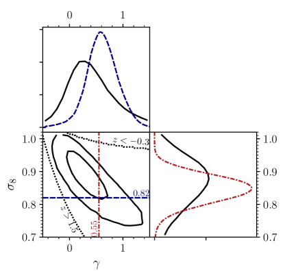
Figure 9: The likelihood degeneracy between the model parameters $\gamma$ and $\sigma_{8}$ today. The contours mark the 1- and 2-$\sigma$ levels. The broken curves show the constraints on $\gamma$ with fixed $\sigma_{8}=0.82$ and on $\sigma_{8}$ with fixed $\gamma=0.55$. The dotted curves indicate the borders of regions requiring extrapolation well beyond the simulation snapshots at $z<-0.3$ or $z>1.5$.

We now adopt the SHAM model without scatter to constrain the growth of structure. For each galaxy sample, we construct a halo sample with matching number density for each one of 12 simulation outputs with snapshot redshifts $0<z_{snap}<1.3$. The correlation functions of the halo samples from each snapshot are over-plotted in the panels of Fig. 7.

The best-fitting snapshot redshift was found for each sample by minimising the $\chi^{2}$ statistic over redshift

$$\chi^{2}=\sum_{i,j}\left(w_{i}^{obs}-w_{i}^{halo}(z)\right)C^{-1}_{ij}\left(w_{j}^{obs}-w_{j}^{halo}(z)\right)$$ (3)

where $i$ and $j$ index the $r_{p}$ bins of the projected correlation function. The analysis was made on scales greater than $r_{min}=1h^{-1}{\rm Mpc}$ to avoid systematic uncertainties in both the observations and simulations. The covariance matrices were inverted using the singular-value decomposition algorithm with a threshold of 0.1 on the relative size of the eigenvalues. Fig. 8 shows the $\chi^{2}$ values and best-fitting redshifts. The uncertainty of the determinations was estimated with the threshold $\Delta\chi^{2}=1$.

The evolution of $\sigma_{8}$ is shown in Fig 8 for alternative gravity models parametrized by the growth index $\gamma$. The mapping is defined using the growth equation $\sigma_{8}(z)$ (Eq. 1). Considering the growth history in the MultiDark cosmology $\sigma_{8}^{MD}(z)$ and an alternative model $\sigma^{\prime}_{8}(z|\gamma)$ we determine the snapshot redshift $z_{MD}$ that satisfies $\sigma_{8}^{MD}(z_{MD})=\sigma^{\prime}_{8}(z|\gamma)$.

In order to test models with high values of $\sigma_{8}$ we would need simulation outputs at scale factors $a>1$ ($z<0$). Since these are not available in MultiDark, we linearly interpolate the correlation function to emulate these outputs. We also extrapolate to higher redshift which is required to test models with low $\sigma_{8}(z)$.

We computed the joint likelihood defined by the $\chi^{2}$ in Eq. 3 of each correlation function measurement as a function of $\sigma_{8}$ and $\gamma$. All other cosmological parameters were implicitly held fixed at the fiducial values of the MultiDark simulation. The likelihood surface is shown in Fig. 9. Some regions of the parameter space require extrapolation of the model well beyond the simulation snapshots. The limits requiring extrapolation to $z<-0.3$ and $z>1.5$ are indicated by the dotted curves in the figure but they are not excluded from the likelihood analysis. The marginalised constraints are $\gamma=0.2^{+0.4}_{-0.3}$ and $\sigma_{8}=0.87\pm 0.07$. By fixing the value of $\sigma_{8}$ today to the MultiDark value $\sigma_{8}=0.82$ we find the growth index $\gamma=0.6^{+0.3}_{-0.2}$. Considering the standard model with $\gamma=0.55$ gives $\sigma_{8}=0.85\pm 0.04$.

6 Discussion and conclusions

At low redshift the distribution of haloes has been shown to be a good proxy for the distribution of galaxies and the SHAM recipe has been a success for modelling galaxy clustering. This is particularly true for galaxy samples that are complete to the characteristic luminosity $L_{\star}$. At higher redshift VIPERS uniquely provides a dataset to complement low redshift studies. Here, we have found that the standard SHAM model without free parameters reproduces the amplitude of the projected correlation function over redshift range $0<z<1$ spanning SDSS and VIPERS.

We tested both luminosity and stellar mass selected sampled in VIPERS constructed to have the same SHAM model. The luminosity-selected samples were found to have a lower clustering amplitude. This supports the claim that stellar mass is a better proxy for the host halo mass. We expect that luminosity becomes less informative at higher redshift due to the greater influence of star formation activity particularly in bluer rest-frame photometry.

Observational scatter in the relationship between stellar mass and the halo $V_{peak}$ property cannot significantly impact the correlation function. We tested scatter in stellar mass at the level of 0.1 dex and found no change in the correlation function and greater levels of scatter is not consistent with the observed shape of the stellar mass function. However, scatter applied to $V_{peak}$ at the level of 0.1 dex does modify the amplitude of the correlation function.

After demonstrating that SHAM can be successfully used to model the VIPERS sample, we apply the re-scaling algorithm proposed by Angulo & White (2010) to test the history of structure formation. The growth history provide direct constraints on alternative cosmological models with modifications to gravity. We estimate the growth index $\gamma$ to be $\gamma=0.6\pm 0.3$ considering SDSS and the VIPERS stellar mass selected samples. The constraint was derived by fixing the value of $\sigma_{8}$ today. Allowing $\sigma_{8}$ to vary significantly reduces the constraining power of the data we consider. The sensitivity of the SHAM prediction depends on number density and we expect that the precision measurements from upcoming photometric and spectroscopic surveys at redshift $\sim 1$ will allow robust constraints on both the normalisation and the redshift dependence of $\sigma_{8}(z)$.

The constraints we find may be compared to those from previous studies based on galaxy peculiar velocities and redshift-space distortions (Guzzo et al., 2008; Song & Percival, 2009; Blake et al., 2011; Beutler et al., 2012; Blake et al., 2013; Johnson et al., 2014; Alam et al., 2017). Galaxy velocities on large scales are sensitive to the derivative of the growth factor $f=-d\log\sigma_{8}(z)/d\log(1+z)=\Omega_{m}(z)^{\gamma}$. Using VIPERS data de la Torre et al. (2017) presented a 20% measurement on $f\sigma_{8}$ in two redshift bins at $z=0.60$ and 0.86. Transforming these constraints to $\gamma$ we find $\gamma=0.57^{+0.3}_{-0.4}$. Hudson & Turnbull (2012) compiled measurements from peculiar velocity and redshift-space distortion surveys and reported the joint constraint $\gamma=0.619\pm 0.054$. Using the BOSS and eBOSS surveys Zhao et al. (2019) found $\gamma=0.469\pm 0.148$. By convention redshift-space distortion analyses fix the amplitude of clustering at high redshift where it is constrained by measurements of the cosmic microwave background. In contrast our method is sensitive to the integrated growth over a period at late time from redshift 1 to 0.

We investigated the effect of systematic uncertainties that would impact the SHAM prediction through the dependence on number density. The sample variance present in the VIPERS sample propagates to the correlation function amplitude at the percent level, and so cannot make a significant contribution to the error. Incompleteness at the  30% level would change the correlation function amplitude by 10%, but we have no evidence for the existence of such a population of missing galaxies. Fig. 2 shows that the sample is incomplete in stellar mass only for the reddest galaxies at high redshift. A significant population of missing red galaxies could affect the clustering amplitude and alter the trend with density shown in Fig. 5; however, we do not expect our results to be significantly biased considering the level of precision of the VIPERS measurements at high redshift. Upcoming surveys such as ESA Euclid will target galaxies in the near infrared and may shed additional light on the importance of stellar mass incompleteness.

The SHAM recipe may be extended in future work to improve the precision of the analysis. Scatter was not needed to fit the VIPERS data, but a degree of intrinsic scatter is expected in the relationship between galaxy and halo properties. More flexible SHAM models can also be used to model samples that suffer from incompleteness (Favole et al., 2016a; Rodríguez-Torres et al., 2017; Favole et al., 2017) or completeness corrections can be inferred from deeper samples. Secondary dependencies that are a signature of assembly bias such as the halo formation time can also improve the precision of the SHAM model (Hearin & Watson 2013; Miyatake et al. 2016; Montero-Dorta et al. 2017; Niemiec et al. 2018; Lin et al. 2016). The additional parameters in these models may be degenerate with the cosmological information we are attempting to extract, but there is a clear way forward if they can be constrained from observations such as weak lensing measurements (Favole et al., 2016a).

References

- Abazajian et al. (2009) Abazajian K. N., et al., 2009, ApJS, 182, 543
- Alam et al. (2017) Alam S., et al., 2017, MNRAS, 470, 2617
- Alonso (2012) Alonso D., 2012, arXiv e-prints, p. arXiv:1210.1833
- Angulo & White (2010) Angulo R. E., White S. D. M., 2010, MNRAS, 405, 143
- Bardeen et al. (1986) Bardeen J. M., Bond J. R., Kaiser N., Szalay A. S., 1986, ApJ, 304, 15
- Baugh (2013) Baugh C. M., 2013, Publications of the Astronomical Society of Australia, 30, e030
- Behroozi et al. (2010) Behroozi P. S., Conroy C., Wechsler R. H., 2010, ApJ, 717, 379
- Behroozi et al. (2013) Behroozi P. S., Wechsler R. H., Wu H.-Y., 2013, ApJ, 762, 109
- Bell & de Jong (2001) Bell E. F., de Jong R. S., 2001, ApJ, 550, 212
- Beutler et al. (2012) Beutler F., et al., 2012, MNRAS, 423, 3430
- Blake et al. (2011) Blake C., et al., 2011, MNRAS, 415, 2876
- Blake et al. (2013) Blake C., et al., 2013, MNRAS, 436, 3089
- Blanton & Berlind (2007) Blanton M. R., Berlind A. A., 2007, ApJ, 664, 791
- Blanton et al. (2003) Blanton M. R., et al., 2003, AJ, 125, 2348
- Blanton et al. (2005) Blanton M. R., et al., 2005, AJ, 129, 2562
- Campbell et al. (2018) Campbell D., van den Bosch F. C., Padmanabhan N., Mao Y.-Y., Zentner A. R., Lange J. U., Jiang F., Villarreal A., 2018, MNRAS, 477, 359
- Cappi et al. (2015) Cappi A., et al., 2015, A&A, 579, A70
- Chaves-Montero et al. (2016) Chaves-Montero J., Angulo R. E., Schaye J., Schaller M., Crain R. A., Furlong M., Theuns T., 2016, MNRAS, 460, 3100
- Conroy et al. (2006) Conroy C., Wechsler R. H., Kravtsov A. V., 2006, ApJ, 647, 201
- Cucciati et al. (2017) Cucciati O., et al., 2017, A&A, 602, A15
- Davidzon et al. (2013) Davidzon I., et al., 2013, A&A, 558, A23
- Davidzon et al. (2016) Davidzon I., et al., 2016, A&A, 586, A23
- Davis & Geller (1976) Davis M., Geller M. J., 1976, ApJ, 208, 13
- Davis & Peebles (1983) Davis M., Peebles P. J. E., 1983, ApJ, 267, 465
- Di Porto et al. (2016) Di Porto C., et al., 2016, A&A, 594, A62
- Favole et al. (2016a) Favole G., et al., 2016a, MNRAS, 461, 3421
- Favole et al. (2016b) Favole G., McBride C. K., Eisenstein D. J., Prada F., Swanson M. E., Chuang C.-H., Schneider D. P., 2016b, MNRAS, 462, 2218
- Favole et al. (2017) Favole G., Rodríguez-Torres S. A., Comparat J., Prada F., Guo H., Klypin A., Montero-Dorta A. D., 2017, MNRAS, 472, 550
- Fritz et al. (2014) Fritz A., et al., 2014, A&A, 563, A92
- Giovanelli et al. (1986) Giovanelli R., Haynes M. P., Chincarini G. L., 1986, ApJ, 300, 77
- Guo & White (2014) Guo Q., White S., 2014, MNRAS, 437, 3228
- Guzzo et al. (1997) Guzzo L., Strauss M. A., Fisher K. B., Giovanelli R., Haynes M. P., 1997, ApJ, 489, 37
- Guzzo et al. (2008) Guzzo L., et al., 2008, Nature, 451, 541
- Guzzo et al. (2014) Guzzo L., et al., 2014, A&A, 566, A108
- Haines et al. (2017) Haines C. P., et al., 2017, A&A, 605, A4
- Harker et al. (2007) Harker G., Cole S., Jenkins A., 2007, MNRAS, 382, 1503
- He et al. (2018) He J.-h., Guzzo L., Li B., Baugh C. M., 2018, Nature Astronomy, 2, 967
- Hearin & Watson (2013) Hearin A. P., Watson D. F., 2013, MNRAS, 435, 1313
- Hudson & Turnbull (2012) Hudson M. J., Turnbull S. J., 2012, ApJ, 751, L30
- Huterer et al. (2015) Huterer D., et al., 2015, Astroparticle Physics, 63, 23
- Johnson et al. (2014) Johnson A., et al., 2014, MNRAS, 444, 3926
- Kaiser (1984) Kaiser N., 1984, ApJ, 284, L9
- Klypin et al. (2016) Klypin A., Yepes G., Gottlöber S., Prada F., Heß S., 2016, MNRAS, 457, 4340
- Landy & Szalay (1993) Landy S. D., Szalay A. S., 1993, ApJ, 412, 64
- Lin et al. (2016) Lin Y.-T., Mandelbaum R., Huang Y.-H., Huang H.-J., Dalal N., Diemer B., Jian H.-Y., Kravtsov A., 2016, ApJ, 819, 119
- Linder (2005) Linder E. V., 2005, Phys. Rev. D, 72, 043529
- Marulli et al. (2013) Marulli F., et al., 2013, A&A, 557, A17
- Mead & Peacock (2014a) Mead A. J., Peacock J. A., 2014a, MNRAS, 440, 1233
- Mead & Peacock (2014b) Mead A. J., Peacock J. A., 2014b, MNRAS, 445, 3453
- Mead et al. (2015) Mead A. J., Peacock J. A., Lombriser L., Li B., 2015, MNRAS, 452, 4203
- Miyatake et al. (2016) Miyatake H., More S., Takada M., Spergel D. N., Mandelbaum R., Rykoff E. S., Rozo E., 2016, Physical Review Letters, 116, 041301
- Montero-Dorta & Prada (2009) Montero-Dorta A. D., Prada F., 2009, MNRAS, 399, 1106
- Montero-Dorta et al. (2017) Montero-Dorta A. D., et al., 2017, ApJ, 848, L2
- Moresco & Marulli (2017) Moresco M., Marulli F., 2017, MNRAS, 471, L82
- Moster et al. (2010) Moster B. P., Somerville R. S., Maulbetsch C., van den Bosch F. C., Macciò A. V., Naab T., Oser L., 2010, ApJ, 710, 903
- Moutard et al. (2016) Moutard T., et al., 2016, A&A, 590, A102
- Niemiec et al. (2018) Niemiec A., et al., 2018, MNRAS, 477, L1
- Norberg et al. (2002) Norberg P., et al., 2002, MNRAS, 332, 827
- Pezzotta et al. (2017) Pezzotta A., et al., 2017, A&A, 604, A33
- Planck Collaboration et al. (2014) Planck Collaboration et al., 2014, A&A, 571, A16
- Pollo et al. (2006) Pollo A., et al., 2006, A&A, 451, 409
- Reddick et al. (2013) Reddick R. M., Wechsler R. H., Tinker J. L., Behroozi P. S., 2013, ApJ, 771, 30
- Rodríguez-Torres et al. (2017) Rodríguez-Torres S. A., et al., 2017, MNRAS, 468, 728
- Rota et al. (2017) Rota S., et al., 2017, A&A, 601, A144
- Scodeggio et al. (2018) Scodeggio M., et al., 2018, A&A, 609, A84
- Silvestri et al. (2013) Silvestri A., Pogosian L., Buniy R. V., 2013, Phys. Rev. D, 87, 104015
- Simha & Cole (2013) Simha V., Cole S., 2013, MNRAS, 436, 1142
- Song & Percival (2009) Song Y.-S., Percival W. J., 2009, J. Cosmology Astropart. Phys., 2009, 004
- Springel et al. (2005) Springel V., et al., 2005, Nature, 435, 629
- Strauss et al. (2002) Strauss M. A., et al., 2002, AJ, 124, 1810
- Trujillo-Gomez et al. (2011) Trujillo-Gomez S., Klypin A., Primack J., Romanowsky A. J., 2011, ApJ, 742, 16
- Vale & Ostriker (2004) Vale A., Ostriker J. P., 2004, MNRAS, 353, 189
- Wang & Steinhardt (1998) Wang L., Steinhardt P. J., 1998, ApJ, 508, 483
- Wechsler & Tinker (2018) Wechsler R. H., Tinker J. L., 2018, Annual Review of Astronomy and Astrophysics, 56, 435
- White & Frenk (1991) White S. D. M., Frenk C. S., 1991, ApJ, 379, 52
- York et al. (2000) York D. G., et al., 2000, AJ, 120, 1579
- Zehavi et al. (2005) Zehavi I., et al., 2005, ApJ, 630, 1
- Zennaro et al. (2019) Zennaro M., Angulo R. E., Aricò G., Contreras S., Pellejero-Ibáñez M., 2019, arXiv e-prints, p. arXiv:1905.08696
- Zhao et al. (2019) Zhao G.-B., et al., 2019, MNRAS, 482, 3497
- de la Torre et al. (2013) de la Torre S., et al., 2013, A&A, 557, A54
- de la Torre et al. (2017) de la Torre S., et al., 2017, A&A, 608, A44