Optically variable active galactic nuclei in the 3 yr VST survey of the COSMOS field

Abstract

Context. The analysis of the variability of active galactic nuclei (AGNs) at different wavelengths and the study of possible correlations among different spectral windows are nowadays a major field of inquiry. Optical variability has been largely used to identify AGNs in multivisit surveys. The strength of a selection based on optical variability lies in the chance to analyze data from surveys of large sky areas by ground-based telescopes. However the effectiveness of optical variability selection, with respect to other multiwavelength techniques, has been poorly studied down to the depth expected from next generation surveys.

Aims. Here we present the results of our r-band analysis of a sample of 299 optically variable AGN candidates in the VST survey of the COSMOS field, counting 54 visits spread over three observing seasons spanning $>3$ yr. This dataset is ¿ 3 times larger in size than the one presented in our previous analysis (De Cicco et al. 2015), and the observing baseline is $\sim 8$ times longer.

Methods. We push towards deeper magnitudes (r(AB) $\sim 23.5$ mag) compared to past studies; we make wide use of ancillary multiwavelength catalogs in order to confirm the nature of our AGN candidates, and constrain the accuracy of the method based on spectroscopic and photometric diagnostics. We also perform tests aimed at assessing the relevance of dense sampling in view of future wide-field surveys.

Results. We demonstrate that the method allows the selection of high-purity (¿86%) samples. We take advantage of the longer observing baseline to achieve great improvement in the completeness of our sample with respect to X-ray and spectroscopically confirmed samples of AGNs (59%, vs. $\sim 15\%$ in our previous work), as well as in the completeness of unobscured and obscured AGNs.
The effectiveness of the method confirms the importance to develop future, more refined techniques for the automated analysis of larger datasets.

1 Introduction

Super-massive black holes (SMBHs) are considered ubiquitous guests in the centers of massive galaxies (e.g., Magorrian et al. 1998; Ferrarese & Merritt 2000). At some point in their lives, they are powered by accreting matter infall; galaxies experiencing such a phase are known as active galactic nuclei (AGNs).

AGN emission is broadband, covering most of the electromagnetic spectrum, as a result of several continuum emission processes plus emission-line features. These features are typically broader and much more prominent than the ones commonly observed in the spectra of inactive galaxies.

Variability is a signature of AGN emission, and is observed at all frequencies, spanning more than twenty orders of magnitude (e.g., Padovani et al. 2017, and references therein). It affects both continuum and line emission to an extent depending on a number of factors: observed spectral range, timescale, presence of radio jets, source luminosity, mass, accretion rate, etc. (e.g., Paolillo et al. 2017). Variations are irregular and aperiodic; their typical timescales range from hours to years, though variations can occasionally be detected on timescales down to minutes or up to $10^{4}$ yr (see, e.g., voorwerpjes, Lintott et al. 2009). Several works over the past decades have widely investigated AGN variability in different wavebands, together with the correlations between variations in different spectral windows (e.g., Ulrich et al. 1997; Gaskell & Klimek 2003). An accurate characterization is nowadays possible thanks to surveys with repeated observations over years/decades. In particular, multivisit surveys have been extensively used to search for unobscured AGNs (e.g., Mushotzky 2004; Klesman & Sarajedini 2007; Trevese et al. 2008; Schmidt et al. 2010; Villforth et al. 2010; MacLeod et al. 2011; Sarajedini et al. 2011; Choi et al. 2014; Graham et al. 2014, and references therein). These surveys are generally characterized by irregular sampling, with observing gaps due to observational constraints. The features of the observed variability depend on several parameters, e.g., baseline, number of visits, observing cadence, chosen band, depth, photometric accuracy.

The next years will see the advent of new-generation telescopes, designed to survey wide sky areas with a high cadence. Among them, the most highly anticipated is undoubtedly the Large Synoptic Survey Telescope (LSST; see, e.g., LSST Science Collaboration et al. 2009). LSST surveys are designed to cover about half the sky. At completion, they will be 10 to 100 times deeper than any present wide-field survey, with hundreds to thousands of time samples. About 90% of LSST’s time will be dedicated to the main survey; the remaining 10% will go into several mini-surveys. These will include ultra-deep observations of 5-10 so-called Deep Drilling Fields (DDFs). The DDFs will target previously surveyed areas, such as COSMOS and the Chandra Deep Field-South (CDFS). For them we can expect up to $\sim 14000$ visits, allowing to reach co-added depths of $ugri\sim 28.5$, $z\sim 28$, and $y\sim 27.5$ mag, over the 10 year survey program. This, combined with the multiwavelength coverage from current and future telescopes, makes the DDFs ideal for AGN studies (see, e.g., Brandt et al. 2018). The first formal survey data from the LSST main survey are expected no sooner than 2023 (best-case scenario). In anticipation, the astronomical community can and must prepare to deal with them, developing fast and reliable classification tools that will be needed to adequately face unprecedented data streams. In this context, we are putting effort into the development and refinement of an effective technique for AGN selection based on their optical variability, with the aim of applying it to wider datasets from surveys to come. We elaborated and tested our selection method analyzing data from the SUpernova Diversity And Rate Evolution (SUDARE; Botticella et al. 2013) survey by the VLT Survey Telescope (VST; Capaccioli & Schipani 2011). SUDARE is a project that aims at analyzing the trend of the rates of different supernova (SN) types in the redshift range $0.3<z<0.8$. In addition, it investigates possible correlations with the properties of the host galaxies, and any dependence of such correlations on redshift and/or on the stellar population the SNe belong to. The survey concerns two distinct, well-known sky areas, the above-mentioned COSMOS field and CDFS. Both regions have been widely surveyed by a large contingent of ground- and space-based observatories: this makes them an ideal testing ground, given the wealth of multiwavelength data, from X-rays to radio, available for the validation of the method.

The SUDARE survey covers 1 sq. deg. for COSMOS and 4 sq. deg. for the CDFS. Observations started in late 2011, and are available in the $g$, $r$, and $i$ bands. In De Cicco et al. (2015) we published the results of the analysis of the first five months of observations (27 visits) for the COSMOS field. Soon after, we presented in Falocco et al. (2015) a similar analysis of the first 2 sq. deg. available for the CDFS: in this case we had 27 visits for one square degree and 22 visits for the other one, spanning five and three months, respectively. We are currently investigating the other half of the surveyed CDFS area, and will present the corresponding results in Poulain et al. (in prep.).

The present paper is dedicated to the analysis of the VST-COSMOS data. The COSMOS campaign has now been extended to a $>3$ yr baseline, doubling the number of observing visits. Here we exploit the longer baseline and increased number of observations, in order to verify the predictions of our previous works and increase the number of detected AGNs. Also, we better constrain the effectiveness of variability selection with respect to other methods, in order to predict the performance of future surveys. We retrieve a larger sample of optically variable AGN candidates due to their typical red-noise variability, thus making progress toward a more complete and effective census of the AGN population in the field.

The present analysis, as well as all of our works published so far, focuses on $r$-band data for both fields. Additional works investigating the other bands, and a combination of all of them, are currently in preparation (see Section 5).

The paper is organized as follows: in Section 2 we describe our dataset; Section 3 illustrates the steps to obtain source catalogs from the various visits, and the reduction process leading to the selection of a robust sample of optically variable AGN candidates. Section 4 deals with the multiwavelength properties of the selected sample, and describes the various diagnostics used to validate the nature of our AGN candidates. In Section 5 we gather together our results and discuss our findings, also comparing them to the ones in De Cicco et al. (2015).

2 The VST-COSMOS data

The VST, located at Cerro Paranal Observatory, is a 2.65 m optical telescope with a 0.938 m-diameter secondary mirror, a modified Ritchey-Chretién configuration, and an alt-azimuth mount. Its detector, OmegaCAM (Kuijken 2011), is a mosaic of 32 CCDs, corresponding to a total of 268 million 15 $\mu$m-size pixels over a $26\times 26$ cm² area. The focal plane scale is $0\aas@@fstack{\prime\prime}214$/pixel, and the corresponding field of view (FoV) is $1^{\circ}\times 1^{\circ}$. The VST-COSMOS observations consist of three observing seasons (hereafter, seasons), covering the span from December 2011 to March 2015, including the data from the season already studied in De Cicco et al. (2015).

Each visit consists of several (usually five, but see Table 1 for details) dithered exposures corresponding to individual $1^{\circ}\times 1^{\circ}$ pointings. Exposure reduction and combination were performed by means of the VST-Tube pipeline (Grado et al. 2012), designed to process VST data. An overview of the processing steps is reported in De Cicco et al. (2015), while a more exhaustive description can be found in Capaccioli et al. (2015). Essentially, the pipeline takes care of overscan correction, bias subtraction, and flat-field correction, together with CCD gain harmonization and illumination correction; astrometric correction and photometric calibration follow, then single exposures are combined together into visits.

The full dataset originally consisted of 65 visits, but we excluded 11 visits from the present analysis, as detailed below; information about the remaining 54 visits, which constitute our final dataset, is reported in Table 1. The first 26 visits in the table cover a five-month baseline and were used for our previous work, described in De Cicco et al. (2015).

A weight map corresponding to each visit accounts for the different noise level of each pixel by associating them a weight, defined as the reciprocal of the pixel variance. As reference, we used the same deep stacked image as in De Cicco et al. (2015), produced as the median of all the exposures having a seeing full width at half maximum (FWHM) $<0\aas@@fstack{\prime\prime}80$; the corresponding exposure time is 19800 s, and the limiting magnitude is $r(\mbox{AB})\approx 26$ mag at $\sim 5\sigma$ above the background r.m.s., while single visits are generally characterized by $r(\mbox{AB})\lesssim 24.6$ mag for point sources, at the same confidence level. Although produced only from the first five months of our observing campaign, this stack is obviously deeper than any of our individual visits, and sufficient for use as a static reference image.

In the present work we focus on $r$-band data only, which have a three-day observing cadence, while for the $g$ and $i$ bands the cadence is $\sim 10$ days; in each case there are several gaps, depending on a number of observational constraints. In the following, magnitudes are quoted in the AB system, unless otherwise stated.

Table 1: COSMOS dataset. Visit number, OB identification number, date, and seeing FWHM for the 54 visits used for the present analysis. Visits are listed in chronological order, and the sequence of their IDs in the first column lacks some numbers because these correspond to the eight visits that we excluded from the analysis (see Section 3.1). Visit 53 was obtained by the combination of ten exposures, for a total exposure time of 3600 s; for all the remaining visits, five exposures were combined together, and the total exposure time is 1800 s.

visit	OB-ID	obs. date	seeing (FWHM)
			(arcsec)
1	611279	2011-Dec-18	$0.64$
2	611283	2011-Dec-22	$0.94$
3	611287	2011-Dec-27	$1.04$
4	611291	2011-Dec-31	$1.15$
5	611295	2012-Jan-02	$0.67$
6	611299	2012-Jan-06	$0.58$
7	611311	2012-Jan-18	$0.62$
8	611315	2012-Jan-20	$0.88$
9	611319	2012-Jan-22	$0.81$
10	611323	2012-Jan-24	$0.67$
11	611327	2012-Jan-27	$0.98$
12	611331	2012-Jan-29	$0.86$
13	611335	2012-Feb-02	$0.86$
14	611351	2012-Feb-16	$0.50$
15	611355	2012-Feb-19	$0.99$
16	611359	2012-Feb-21	$0.79$
17	611363	2012-Feb-23	$0.73$
18	611367	2012-Feb-26	$0.83$
19	611371	2012-Feb-29	$0.90$
20	611375	2012-Mar-03	$0.97$
21	611387	2012-Mar-13	$0.70$
22	611391	2012-Mar-15	$1.08$
23	611395	2012-Mar-17	$0.91$
24	768813	2012-May-08	$0.74$
25	768817	2012-May-11	$0.85$
26	768820	2012-May-17	$0.77$
28	986611	2013-Dec-27	$0.72$

visit	OB-ID	obs. date	seeing (FWHM)
			(arcsec)
29	986614	2013-Dec-30	$1.00$
30	986617	2014-Jan-03	$0.86$
31	986620	2014-Jan-05	$0.81$
32	986626	2014-Jan-12	$0.73$
33	986630	2014-Jan-21	$1.18$
34	986633	2014-Jan-24	$0.80$
37	986648	2014-Feb-09	$1.28$
38	986652	2014-Feb-19	$0.89$
39	986655	2014-Feb-21	$0.93$
40	986658	2014-Feb-23	$0.81$
41	986661	2014-Feb-26	$0.81$
42	986664	2014-Feb-28	$0.77$
44	986670	2014-Mar-08	$0.91$
45	986674	2014-Mar-21	$0.96$
46	986677	2014-Mar-23	$0.92$
47	986680	2014-Mar-25	$0.66$
48	1095777	2014-Mar-29	$0.89$
49	1095783	2014-Apr-04	$0.58$
50	986683	2014-Apr-07	$0.61$
51	1136410	2014-Dec-03	$1.00$
53	1136457	2015-Jan-10	$0.71$
55	1136481	2015-Jan-28	$0.90$
56	1136490	2015-Jan-31	$0.73$
57	1136503	2015-Feb-15	$0.70$
60	1136531	2015-Mar-10	$0.80$
61	1136540	2015-Mar-14	$0.84$
62	1136543	2015-Mar-19	$1.00$
stacked	-	-	$0.67$

3 Selection of variable sources

As a first step, we visually inspected each visit in our dataset in order to verify its quality: this led to the exclusion of three visits because of severe aesthetic artifacts and defects.

The method we adopt to identify optically variable sources, and hence define our sample of AGN candidates, follows the approach proposed by Trevese et al. (2008).

3.1 Catalog production and aperture selection

A catalog of sources was obtained from each visit making use of SExtractor (Bertin & Arnouts 1996): this contains a number of parameters for each object, including positional coordinates, half-light radii, and magnitudes through a set of fixed apertures. We fed the above-mentioned weight maps to SExtractor so that, in the process of catalog extraction, the different quality of each pixel in each visit is taken into account.

AGN identification requires an aperture size allowing the collection of the bulk of the flux from the nucleus of a galaxy, while minimizing the contribution from the host galaxy itself and possible nearby sources. In De Cicco et al. (2015) we measured the source flux within a 2″-diameter, which typically encloses $\approx 70\%$ of the flux from a point-like object, and then, in order to take into account the effect of seeing, we computed corrective factors for each visit making use of growth curves of reference stars. A growth curve shows how the fraction of flux collected from a source changes as a function of the aperture size.

Here we adopt a different approach, following Trevese et al. (2008), which essentially consists of normalizing all visits to a reference one. In our case we chose visit 49, which has the second-best seeing (see Table 1) and is free from significant aesthetic artifacts . Then, for each visit, we selected all the sources with 2″-diameter aperture r(AB) magnitudes in the range 16–21 (so as to avoid very bright/saturated or faint and noisy objects) and computed the average magnitude difference $\langle\Delta\mbox{\tiny{mag}}\rangle$ with respect to the reference visit. The catalogs of sources obtained from different visits were matched requiring the distance between positional coordinates to be $<1\arcsec$. We subtracted from all 2″-aperture magnitudes in each visit the corresponding corrective factor in order to account for seeing and calibration differences. The magnitude difference between visits 3 and 49, for all the sources in the field, before and after the correction, is shown in Fig. 1 as an example.

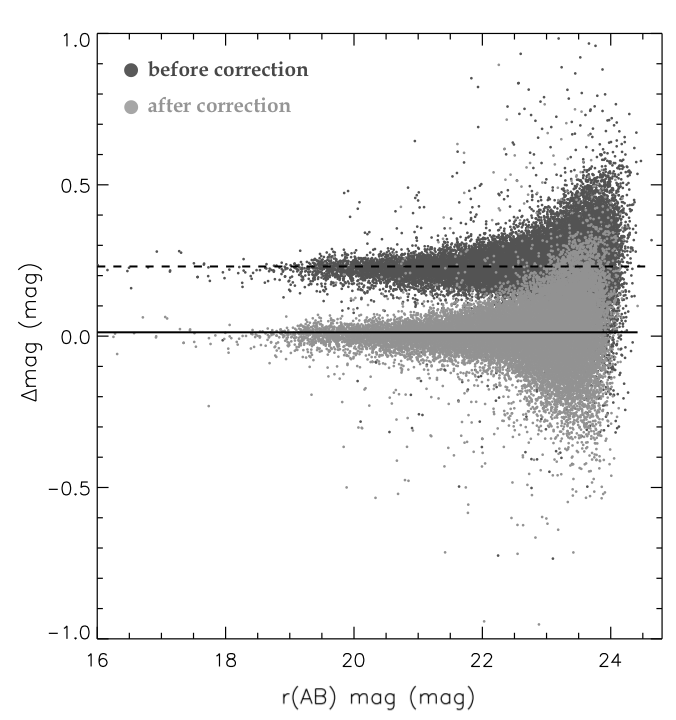
Figure 1: Magnitude difference between visit 3 and visit 49, which is used as a reference. Though all the sources with an available measurement of their magnitude are shown, the ones used to determine the aperture corrective factors have r(AB) magnitudes in the range 16–21. Dark and light gray dots represent magnitudes before and after the correction, respectively; similarly, the dashed and solid lines correspond to the average magnitude difference before and after the correction, respectively. The first defines the corrective factor which, in this case, is $\approx 0.22$. The obtained value varies depending on the visit seeing, being larger for higher seeing values; visit 3 has a seeing value of 1$\aas@@fstack{\prime\prime}$04, which is one of the largest in our set of visits.

As a further step, we computed the r.m.s. deviation $\sigma_{\Delta\mbox{\tiny{mag}}}$ of $\Delta\mbox{\tiny{mag}}$ for each visit, in order to quantify the calibration uncertainty with respect to the reference visit. $\sigma_{\Delta\mbox{\tiny{mag}}}$ for each visit is reported in Fig. 2. We decided to exclude from our dataset the visits characterized by $\sigma_{\Delta\mbox{\tiny{mag}}}$ values higher than 0.05; these correspond to eight visits, represented by the most scattered points in the figure. The adopted limit is arbitrary and indeed there are some excluded visits very close to the threshold. We tested how the inclusion of these four visits would affect the analysis. Although their inclusion would add a few ($<10$) more sources to the sample of optically variable AGN candidates, it would also introduce several dozens of contaminants. Thus, although excluding these visits may be considered a conservative approach, their exclusion did not significantly impact our results.

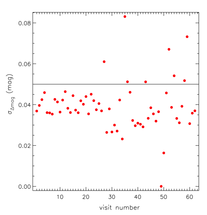
Figure 2: $\sigma_{\Delta\mbox{\tiny{mag}}}$ for each visit. The sources used to determine the aperture corrective factors have r(AB) magnitudes in the range 16–21. The points above the black line correspond to the eight visits that we excluded from our dataset.

s

3.2 Defects and masks

Observations of the COSMOS field from the first season correspond to the very beginning of VST activity, and various early visits turned out to be affected by a number of defects in the detector electronics, as well as aesthetic artifacts; VST data-users, including us, had to address them for the first time, and the most natural path to follow resulted in a conservative approach. Some of the problems arose from a poor knowledge of the detector response, and were fixed in the following months. In particular, the most relevant problem was a CCD characterized by random variations in its gain factor, which resulted in a large concentration of fake sources in the corresponding area of the detector; this led to the exclusion of the image region corresponding to that CCD from the affected visits. Similarly, other regions were excluded in some or all the visits, depending on the circumstances. Examples are the regions at the edge of each visit (corresponding to a $\approx 2\arcmin$–$4\arcmin$ width each side), characterized by a very low signal-to-noise ratio (S/N), satellite tracks, regions affected by reflections of scattered light, and –last but not least– bright star halos. The last ones are a common feature in wide-field surveys, and constitute the main problem that we had to address by applying suitable masks to the images at issue. Bright stellar halos and spikes were masked making use of the regions produced by the Pulecenella code developed by Huang et al. (2011). These initial masks were improved upon by adding, when necessary, additional eye-selected regions to be excluded, for each visit.

Specifically, for one individual visit, an additional region affected by reflections of scattered light was masked. Satellite tracks were not masked, but the potential problems they could cause were minimized by resorting to a $\sigma$-clipping algorithm (see Section 3.3). The masking process reduced the number of objects in each catalog by a couple tens of thousands, representing 20%–25% of the whole source catalog depending on the seeing value (higher seeing required larger masked areas).

3.3 The sample of AGN candidates

We cross-matched the catalogs of sources obtained for each visit by matching positional coordinates within a $1\arcsec$ radius, in order to get the light curves of all the detected objects. Source separations are $<$ 0$\aas@@fstack{\prime\prime}$26 in 95% of the cases. The master catalog thus obtained includes all the variable and non-variable sources detected in at least two visits and with an average magnitude r(AB) $\leq 23.5$ mag. Our previous work focused on sources with a r(AB) $\leq 23$ mag; here we extend the sample down to fainter magnitudes, consistent with the single-visit completeness limit.

The master catalog contains 25452 sources, including a number of objects detected in just a few visits, many of these are either fast transients and/or more likely spurious sources. In order to minimize contamination from such objects, we make a further cut and require the sources in our final catalog to be detected in at least half the visits.

We note that we adopt a different criterion than in De Cicco et al. (2015), where we required sources to be detected in at least 20% of the visits. The minimum number of visits is somewhat arbitrary, as it depends on the type of source to detect/exclude and its variability. Here we increased the minimum visit requirement based on our experience with the first five months of data, and considering the longer time span of our light curves (which increases the likelihood of detecting variability from fainter AGNs). We find that anyway 90% of the sources in our master catalog are detected in at least half the visits. This percentage would rise to 99% if we required sources to be detected in 20% of the visits, but the sample of variable AGN candidates would be almost the same as the one we obtain with the adopted threshold, with a couple dozens additional sources that would be mostly contaminants. We therefore opted for the more conservative threshold.

The number of visits in each light curve also affects the detection significance for variable sources due to the different number of degrees of freedom in each light curve (see discussion in De Cicco et al. 2015). To assess the relevance of this effect we performed simulations including each time a different number of visits, and we found that the detection threshold for variable sources differs by less than 15% between sources detected in all visits and those detected in just half of them.

The applied selection criteria returned a sample of 22927 sources (hereafter, the main sample); we point out that this includes both variable and non-variable sources.

In order to define a variability threshold, we computed the average magnitude $\langle{\mbox{mag}}_{i}^{lc}\rangle$ and the corresponding r.m.s. deviation $\sigma_{i}^{lc}$ for each source $i$ from the corresponding light curve:

$$\small\langle{\mbox{mag}}_{i}^{lc}\rangle=\frac{1}{N_{vis}}\sum_{j=1}^{N_{vis}}\mbox{mag}_{i}^{j}\mbox{ ,}\qquad\sigma_{i}^{lc}={\left[\frac{1}{N_{vis}}\sum_{j=1}^{N_{vis}}{(\mbox{mag}_{i}^{j}-\langle{\mbox{mag}}_{i}^{lc}}\rangle)^{2}\right]}^{\frac{1}{2}}\mbox{,}$$ (1)

where the superscript $lc$ stands for “light curve”, $j$ runs through the visits, and $N_{vis}$ is the number of visits where we detect the source $i$. Both $\langle{\mbox{mag}}^{lc}\rangle$ and $\sigma^{lc}$ were obtained through a $\sigma$-clipping algorithm, rejecting $>5\sigma$ outliers, in order to minimize spurious contributions to magnitude variations due, for instance, to residual aesthetic defects (e.g satellite tracks, cosmic rays, stellar diffraction spikes, etc.).

Once we measured the properties of all light curves in our main sample, we extracted the sample of variable sources. We initially define as variable candidates all sources exhibiting a $\sigma^{lc}$ in excess of the 95th percentile of the $\sigma^{lc}$ distribution, over a running 0.5 mag-wide bin centered on the magnitude of each source. We identified 482 sources ($2.1\%$ of the main sample) above the variability threshold, which constitute our preliminary sample of AGN candidates. Figure 3 shows the variability threshold and the sample of AGN candidates in the plane of $\sigma^{lc}$ vs. $\langle{\mbox{mag}}^{lc}\rangle$.

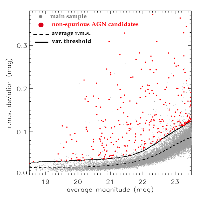
Figure 3: Light curve r.m.s. $\sigma^{lc}$ as a function of the average magnitude $\langle{\mbox{mag}}^{lc}\rangle$ for all the sources in the main sample (small gray dots). The dashed line represents the running average of the r.m.s., while the solid line defines the variability threshold. Objects above the threshold are considered to be variable, and large red dots identify non-spurious AGN candidates (flag 1 or 2, see further in the text).

We expect the variability of some sources in our preliminary sample to be spurious due to a number of factors: contamination from a close companion; the irregular morphology of some galaxies, which makes it difficult to identify the source centroid in the visits with the worst seeing values; the presence of problematic areas of the detector (e.g., hot pixels) or noise-dominated regions (e.g., the edges of a frame) where sources happen to fall. We also expect our sample to include a number of contaminants, such as variable stars and transient events (e.g., SNe). The identification and analysis of SNe in our dataset is currently ongoing (Ragosta et al., in prep.); in De Cicco et al. (2015) we measured a $14\%$ contamination rate due to SNe in our final sample of variable sources.

Our preliminary sample of optically variable sources includes 90 objects that suffer from blending with neighboring galaxy at least in the visits with worse seeing. We inspected the snapshots of each source in each visit, and they revealed that the centroid position can vary substantially, migrating from one object to the other, depending on the visit. This means that, in either case, the corresponding measured flux is possibly wrong, hence we excluded them from our analysis. This leaves 392 candidates. In order to identify and reject spurious sources and contaminants, we visually inspected the snapshots of each source in each visit, and flagged sources with a quality label ranging from 1 to 3 on the basis of the following guidelines:

1. strong candidate; no problems or defects detected (232 sources);

2. likely variable candidate; neighbor potentially affecting the source, or minor problems detected (67 sources);

3. very doubtful variability; likely spurious (93 sources).

Sources are flagged as 3 either because of their irregular shape (43 objects), which does not allow reliable identification of a center, or because of the presence of a nearby saturated object (50 objects); in this case we used the same empirical selection criterion that we set in our previous work, and required the centroid-to-centroid distance to be $\leq$ 2″ and the magnitude difference of the two sources to be $<1.5$ mag for a source to be a flag 3, as we assumed that, in such a case, the light from one source strongly affects the other.

We point out that the sample cleaning process can be automated in part using SExtractor flags and other diagnostics to exclude a priori sources with close neighbors, those with cross-contamination, and so on. In this case we resorted to a manual approach due to the limited number of candidates to inspect and to have a reference sample to optimize the automatic procedure in the future; the implementation is already in progress for our already-mentioned follow-up work combining $g$, $r$, and $i$ light curves, and will be an unavoidable approach when dealing with any future larger sample.

In Fig. 4 we present one source per class as an example; images for flags 1 and 2 are from the visit with the second-best seeing, while for flag 3 we show an image from the worst-seeing visit, in order to give an idea of how hard it is to identify the source above the complex background due to the bright extended neighbor. The variability analysis that we describe in the following is limited to the sources labeled 1 or 2 (hereafter, the robust sample), consisting of 299 sources and hence constituting $1.3\%$ of the main sample and 62% of the initial AGN candidates with r(AB) mag $\leq 23.5$ mag.

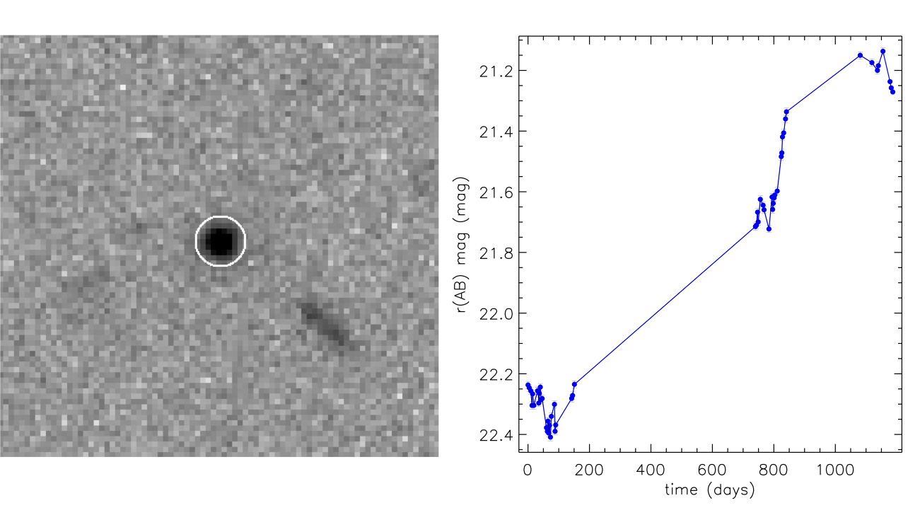
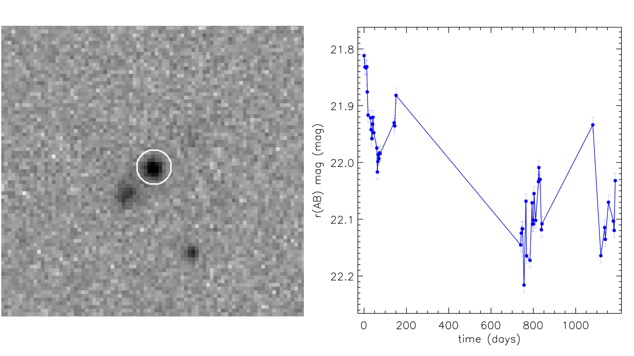
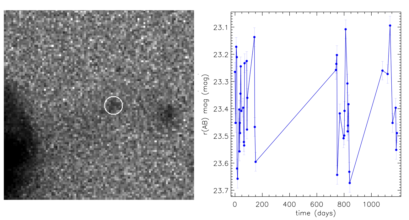
Figure 4: Examples of variable AGN candidates assigned to different quality classes, with corresponding light curves. The images in the upper and middle panel are from visit 49, which has the second-best seeing; the image in the lower panel is from visit 33, which has the worst seeing. White circles correspond to the $2\arcsec$-diameter aperture and are centered on the average object coordinates. Objects labeled 1 (upper panel) are generally isolated and free from aesthetic defects. In the case of the objects belonging to class 2 (middle panel), potential problems (e.g., the presence of a neighbor) must be taken into account. Objects labeled 3 (lower panel) are probably spurious variable sources; the case of a source lying in the halo of an extended and bright neighbor (on the far left) is shown as an example: from the corresponding light curve, we can see that its erratic variability, well in excess of the photometric error, is likely due to an improper subtraction of the variable background due to the bright neighbor. The error bars for each source are defined as the 95% uncertainty on the source magnitude.

4 Validation and characterization of the AGN candidates

In the present section we investigate the nature and properties of the sources in our robust sample, aiming at confirming AGNs and at classifying as many of the remaining sources as possible. We intend to assess to what extent optical variability is a reliable indicator of the presence of an AGN, and hence a powerful alternative to other more expensive and/or time-consuming techniques (e.g., X-ray identification) usually employed in the search for AGNs.

Due to the widespread literature about the COSMOS field, several catalogs at different wavelengths are available for most of the sources, and classification already exists for part of our sample. This allowed us to validate our results by means of extensive ancillary data.

4.1 X-ray counterparts

X-ray emission, especially if coupled with variability, is the strongest and most reliable indicator of the presence of an AGN (e.g., Brandt & Alexander 2015). In the present work we made use of two X-ray catalogs of COSMOS sources to identify possible X-ray counterparts for our main sample:

• the catalog containing optical and near-infrared (NIR) counterparts of the sources in the Chandra-COSMOS Legacy Catalog (Marchesi et al. 2016; Civano et al. 2016), consisting of 4016 X-ray emitters over a 2.2 sq. deg. area; the catalog is the result of a 4.6 Ms program with an exposure of $\simeq 160$ ks in the central 1.5 sq. deg. and $\simeq 80$ ks in the surrounding area. The limiting depth corresponds to fluxes of $2.2\times 10^{-16}$ erg cm^-2 s^-1, $1.5\times 10^{-15}$ erg cm^-2 s^-1, and $8.9\times 10^{-16}$ erg cm^-2 s^-1 in the 0.5–2, 2–10, and 5–10 keV bands, respectively. The catalog provides a considerable volume of information, including optical counterparts for 3899 ($97\%$) of the 4016 sources, spectroscopic classification (broad-line AGN, i.e., BLAGN; non-BLAGN; star) for $\approx 42\%$ of the sample, and photometric classification (obscured/unobscured AGN; galaxy; star) based on the fitting of the spectral energy distribution (SED) for $96\%$ of the sample;

• the XMM-COSMOS Point-like Source catalog (Brusa et al. 2010), including 1674 X-ray sources with optical counterparts. The corresponding observations ($\simeq 60$ ks) in this case are shallower and a little less extended (2 sq. deg. area) than the Chandra-COSMOS Legacy Survey; the flux limits in the 0.5–2  keV, 2–10  keV, and 5–10  keV energy bands are, respectively, $\approx 1.7\times 10^{-15}$ erg cm^-2 s^-1, $\approx 9.3\times 10^{-15}$ erg cm^-2 s^-1, and $\approx 1.3\times 10^{-14}$ erg cm^-2 s^-1 over $90\%$ of the area. Spectroscopic classification (BLAGN; narrow-line AGN, i.e., NLAGN; normal/star-forming galaxy) is available for about half the sample, and a best-fit SED template by Salvato et al. (2009) is provided for $97\%$ of the sample. Though this catalog is far shallower than the Chandra catalog, it provides some useful details about the nature of the sources (see Section 4.2).

The two X-ray catalogs provide information for 1815 X-ray sources in the VST-COSMOS FoV (excluding masked areas), with coordinates for their optical counterparts reported in the X-ray catalogs themselves. Nevertheless, not all of them have a VST counterpart. Specifically, we found:

• 719 X-ray sources with magnitude $r$(AB) $<23.5$ mag and a VST counterpart;

• 575 sources with magnitude $r$(AB) $>23.5$ mag, hence not taken into account in what follows;

• 512 sources with a VST counterpart but detected only in a few visits since they are close to the detection limit, and hence excluded from the main sample, according to the visit threshold we set (see Section 3.3);

• five sources with $r$(AB) $<23.5$ mag and with a very close, very bright neighbor, which prevented the detection in VST data;

• three sources for which we find a VST counterpart with a matching radius larger than $1\arcsec$;

• one source which appears very blurred in the VST images, and with no magnitude estimate in either of the two X-ray catalogs.

The sample of X-ray sources that have a VST counterpart and fulfill our selection criteria hence consists of 719 objects (hereafter, the X-ray sample), or $3\%$ of the 22927 sources in the main sample. The match of the robust sample with the X-ray sample revealed 250 AGN candidates (83.6% of the robust sample: hereafter, X-ray emitting variable AGN candidates) with an X-ray counterpart; this implies that 250 out of 719 X-ray sources with bright optical counterparts (35%) appear optically variable in our catalog.

All but one of the 250 X-ray emitting variable AGN candidates have an X-ray counterpart in the deeper Chandra catalog, and we thus preferentially quote the Chandra values.

The ratio of the X-ray-to-optical flux (X/O) of a source is traditionally defined as (Maccacaro et al. 1988)

$$X/O=\log(f_{\scriptscriptstyle{X}}/f_{opt})=\log f_{\scriptscriptstyle{X}}+\frac{\mbox{mag}_{opt}}{2.5}+C\mbox{ ,}$$ (2)

where $f_{\scriptscriptstyle{X}}$ is the X-ray flux measured in a chosen energy band, while $\mbox{mag}_{opt}$ is the optical magnitude at a chosen wavelength, and $C$ is a constant which depends on the magnitude system adopted for the observations; in our case, the X-ray fluxes are from the Chandra catalog and are measured in the 2–10 keV band, while the optical magnitudes are the VST r(AB) magnitudes; this leads to a value for the constant $C=1.0752$. Stars and inactive galaxies typically exhibit X/O $<-2$ (e.g., Mainieri et al. 2002; Xue et al. 2011), while AGNs are usually characterized by $-1\leq$ X/O $\leq 1$, hence the X/O constraints on our sources can help unveil their nature. In Fig. 5 we show the hard (2–10 keV) X-ray flux vs. r-band magnitude for the sources in the robust sample with an X-ray counterpart. It is apparent that all but six of the X-ray emitting variable AGN candidates lie in the AGN locus, while six sources have an X/O $>1$; following Civano et al. (2012), we consider all 250 X-ray emitting variable AGN candidates as AGNs due to their X/O values. This means that, if no additional information about our robust sample were available, on the sole basis of the X/O diagram we could be confident that $83.6\%$ (250/299) are indeed AGNs, representing a lower limit on the purity of our sample. We define the completeness as the ratio of the sources that we confirm as AGNs (250 objects) and the number of AGNs in our X-ray sample (i.e., the X-ray sources that lie in the AGN region on the X/O diagram, namely 668 sources). This results in a fraction of 37% (250/668) completeness. We point out that there is always some degree of uncertainty in the definition of the X/O of a source, because of the intrinsic variability of the source itself combined with the non-simultaneity of the X-ray and optical observations (e.g., Paolillo et al. 2017; Chiaraluce et al. 2018), and the changing contributions from the host galaxy in the optical band as a function of redshift (see, e.g., Fig. 3 of Alexander et al. 2002).

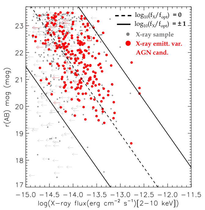
Figure 5: r(AB) magnitude vs. hard (2–10 keV) X-ray flux for the 250 X-ray emitting variable AGN candidates (large red symbols denote Chandra detections, open box denotes XMM detection). The small grey symbols denote the remainder of the X-ray sample. Leftward arrows indicate that only upper limits of the X-ray flux values are available. The dashed line corresponds to X/O $=0$; the lower and upper solid lines represent X/O $=-1$ and X/O $=1$, respectively, and define the AGN locus.

4.2 Spectroscopic and photometric classification

In Section 4.1 we mentioned that both Chandra and XMM catalogs provide a spectroscopic and a photometric classification for part of the X-ray emitters in each of the catalogs. In the first one, objects with a spectroscopic classification are labeled as BLAGNs if their spectra show at least one broad (FWHM $>2000$ km s^-1) emission line, while non-BLAGNs could be NLAGNs or star-forming galaxies: this is either because most of the sources at issue are characterized by low S/N spectra, or because the waveband in which the spectra are obtained does not allow utilization of optical emission line diagnostics which would help separating the two classes of objects. The photometric classification, instead, is derived through best-fit templates of the broadband SEDs, and sources are divided into unobscured AGNs, obscured AGNs, inactive galaxies, and stars. A cross-match of the two classifications confirmed that $82\%$ of the BLAGNs correspond to unobscured AGNs; the match is not higher because BLAGN SEDs, especially for low-luminosity AGNs, suffer from stellar light contamination; non-BLAGNs are matched to obscured AGNs in $23\%$ of the cases and to galaxies in $74\%$ of the cases (Marchesi et al. 2016).

The XMM catalog classifies sources as BLAGNs, NLAGNs, and inactive galaxies. BLAGNs must fulfill the same criterion as in the Chandra catalog; sources flagged as NLAGNs typically have spectra characterized by unresolved high-ionization emission lines with line ratios suggesting AGN activity, while inactive galaxy spectra are generally consistent with those of star-forming or normal galaxies, and have rest-frame hard X-ray luminosity $L_{X}<2\times 10^{42}$ erg s^-1, when detected in the hard X-rays; part of the best-fit SED templates correspond to unobscured (also known as Type 1) and obscured (Type 2) AGNs (Brusa et al. 2010).

In the VST X-ray sample (see Section 4.1) 600 out of 719 sources have a spectroscopic classification from either of the two catalogs; moreover, all but six out of 719 sources have a photometric classification. Among the spectroscopically classified objects, we find 243 unobscured AGNs and 140 obscured AGNs, based on the Chandra catalog and always adopting the spectroscopic over photometric classification. While the definitions for unobscured AGNs are the same in the two X-ray catalogs, the label “non-BLAGN” in the Chandra catalog is ambiguous (see details in Section 4.1), and hence not sufficient to classify a source. The robust sample also includes 11 sources spectroscopically classified as stars.

Our 250 X-ray emitting variable AGN candidates are spectroscopically classified as: 200 unobscured AGNs; 25 obscured AGNs; two stars; five sources with uncertain classification, including two possible inactive galaxies; 18 unclassified sources. Nonetheless, we note that 17 out of the 23 sources not classified as obscured/unobscured AGNs (18 unclassified + 5 uncertain), including the two possible inactive galaxies, have X-ray luminosities $L_{X}>3\times 10^{42}$ erg s^-1, indicative of AGNs (e.g., Brandt & Hasinger 2005); moreover, by selection all 23 sources lie on the AGN stripe in the X/O diagram. This means that spectroscopic information alone allows to identify 225 AGNs and two stars; combining this information with the X/O information, and taking into account the X-ray luminosities, we can therefore classify as AGNs 248 out of the 250 X-ray emitting variable AGN candidates, excluding the two stars, but including the two possible inactive galaxies.

The completeness of variability selection with respect to the spectroscopically confirmed sample is defined as the ratio of spectroscopically confirmed AGNs (in the robust sample) to the expected AGNs (in the X-ray sample), and is $59\%$ (225/383) while, if computed separately for unobscured and obscured AGNs, we obtain 200/243 = $82\%$ and 25/140 = $18\%$, respectively. These fractions are much higher than those reported in De Cicco et al. (2015); this is one of the main results of this work and will be discussed further in Section 5.

4.3 Color-based classification

Diagrams comparing source colors are widely used to disentangle different classes of objects (see, e.g., Boutsia et al. 2009; Nakos et al. 2009), based on the fact that sources tend to have distinct SEDs and occupy distinct loci on such diagrams, depending on their nature.

In order to obtain color diagrams, we made use of data from two additional COSMOS catalogs:

• the already-mentioned COSMOS2015 catalog (Laigle et al. 2016), which contains photometry and physical parameters for more than half a million objects in several filters (including intermediate- and narrow-band ones) spanning a wide range of wavelengths, and also provides matches with optical, X-Ray, UV, IR, and radio catalogs, as well as previous versions of the COSMOS multiband catalog. We use this catalog to obtain the magnitudes we need in the $r$, $z$, and $k$ bands, down to a magnitude r(AB) $\approx 28$ mag.

• the COSMOS ACS catalog (Koekemoer et al. 2007; Scoville et al. 2007) from the Hubble Space Telescope (HST), obtained from 575 pointings of the Advanced Camera for Surveys (ACS). This catalog is mainly used because it provides a morphological classification based on the SExtractor stellarity index, ranging from 0 (extended source) to 1 (point-like source). Given the exquisite HST resolution, this catalog allows us to better distinguish galaxies from stars and quasars, as discussed below.

4.3.1 Optical-NIR diagnostic

Nakos et al. (2009) show that the use of the r-z vs z-K diagram is very effective in distinguishing stars from extended galaxies. The former form a tight sequence, while the latter tend to occupy a bluer NIR scattered region. Our r-z vs. z-K diagram is shown in Fig. 6; color information is available for 296 out of 299 sources. When we overplot our variable AGN candidates on this diagram, there is a large overlap with the galaxy region that extends to redder colors, although they are on average more compact than galaxies, as revealed by their stellarity index.

Based on this, and the stellar locus limit introduced by Nakos et al. (2009), we exclude from our robust sample nine stellar sources (3% of 299 variable AGN candidates) that lie on the stellar sequence far from the galaxy locus. A few additional AGN candidates lie in the overlap region between stars and galaxies, so we cannot assess their nature based on this diagram alone. We note that the number of stars detected over our three-year survey is significantly higher than in our first five-month analysis, where we detected no variables on the stellar locus of the r-z vs. z-K diagram, and is also larger than the fraction of stars found in the first 2 sq. deg. of the VST-CDFS survey, analyzed in Falocco et al. (2015). This is due to some extent to the longer temporal baseline and the fainter magnitude limit, but mostly to our more relaxed selection criterion (95th percentile threshold, see Section 3.3) compared to the one used in our previous works, which allowed lower contamination.

Near-infrared photometry allows to separate stars from galaxies better than traditional optical colors (e.g., U-B vs. B-V diagrams), and to approximately identify an AGN locus, where point-like sources with colors typical of galaxies are located. Nonetheless, we do see a non-negligible fraction of variable AGNs –particularly optically redder and/or fainter ones, where the host galaxy contamination is more severe or where the nucleus is obscured– whose colors and stellarity are consistent with those of inactive galaxies and hence are hard to identify by means of this diagram alone. A caveat here is that this diagnostic is prone to larger contamination than the diagnostics based on X-ray properties, since stars, galaxies, and AGNs have significant overlaps. As a consequence, we only use it to assess the extent of stellar contamination, which corresponds to the above mentioned 3%.

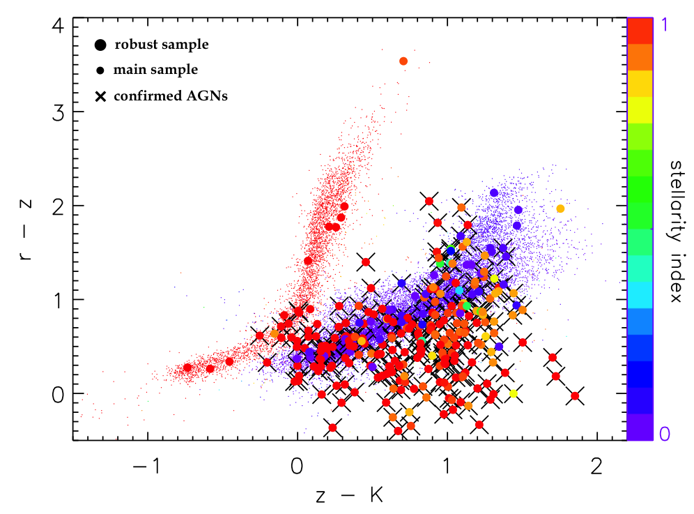
Figure 6: r-z vs. z-K diagram for the 296 out of 299 AGN candidates in the robust sample (large dots) for which $r$, $z$, $K$ magnitudes and stellarity index are available. Small dots represent all the objects detected in the VST-COSMOS field for which HST stellarity indices and optical/NIR color information are available, and are shown as a reference population. Both large and small dots are color-coded according to their stellarity index (right vertical axis). Crosses indicate X-ray emitting variable AGN candidates confirmed by their X-ray properties. It is apparent that the small dots in the plot define two distinct loci: one for stars (red), and one for galaxies (violet). A third class of objects, i.e., quasar-like AGNs, is identified from the large dots, corresponding to sources approximately near or below the galaxy locus but mostly with stellarity indices typical of compact sources. Approximately 6% of the main sample sources shown in Fig. 6 are located in the above-mentioned AGN locus, but are not part of our robust sample of AGN candidates as they are below the variability threshold in the diagram shown in Fig. 3. None of these sources has an X-ray counterpart in the X-ray sample, and 96% of them are extended sources based on their stellarity. $K_{s}$ magnitudes are by McCracken et al. (2010).

4.3.2 Mid-infrared diagnostic

Lacy et al. (2004) proposed a color-color diagnostic based on the use of mid-infrared (MIR) fluxes (3.6, 4.5, 5.8, and 8.0 $\mu$m) from the Infrared Array Camera (IRAC; e.g., Fazio et al. 2004) of the Spitzer Space Telescope to select AGNs. The $8.0\mbox{ }\mu m/4.5\mbox{ }\mu m$ and the $5.8\mbox{ }\mu m/3.6\mbox{ }\mu m$ ratios allow separation of sources whose continuum emission is dominated by different components, such as stellar emission, dust reprocessing in star-forming regions, or nuclear dust heated by the central AGN. In Fig. 7 several distinct loci are visible. Stars and low-redshift passive galaxies are characterized by bluer colors on both axes, and define the denser region that can be observed in the lower-left part of the plot. Star-forming galaxies with $z\lesssim 1.5$ are preferentially found on a roughly vertical sequence corresponding to colors with $5.8\mbox{ }\mu m/3.6\mbox{ }\mu m<0.1$ and $8.0\mbox{ }\mu m/4.5\mbox{ }\mu m>0.2$. Finally, quasars and AGN-dominated galaxies define a diagonal locus characterized by red colors on both axes. By defining color criteria, Lacy et al. (2004) delineated boundaries where AGNs generally are located on the diagram; this region was slightly modified in Lacy et al. (2007), and we refer to it here and in the following (hereafter, the Lacy region).

As shown by Donley et al. (2012), the Lacy region includes most galaxies with a MIR AGN contribution $\gtrsim 40\%$, but is not free from contamination by inactive galaxies. A more restrictive selection criterion was proposed by Donley et al. (2012), aiming at reducing heavy contamination by star-forming galaxies, which is particularly problematic at high redshift ($z\gtrsim 2$). Donley et al. (2012) make use of simulations to construct IRAC colors of composite SEDs with different AGN contributions, in the redshift range 0–3, and show that, as the AGN contribution becomes dominant, the IRAC colors of the corresponding sources move onto a the locus where sources with perfect IRAC power-law SEDs would lie (hereafter, the Donley region).

Based on the analysis in Falocco et al. (2015), we show our version of the IRAC diagram in Fig. 7, which includes the AGN selection boundaries from both Lacy et al. (2007) and Donley et al. (2012), in order to allow a comparison. IRAC fluxes are from the COSMOS2015 catalog, and are available for 273 out of the 299 sources in our robust sample. We find that $82\%$ (223/273) of the AGN candidates with IRAC fluxes lie within the Lacy region, including two sources confirmed ex novo, i.e., not confirmed by any of the previous diagnostics. We caution that this does not constitute a purity estimate since the Lacy region is also known to include non-AGN contaminants. We assess the completeness of our variability selection with respect to MIR diagnostics, recovering 18% (223/1235) and 55% (138/249) of the sources that fall in the Lacy and Donley region, respectively. However, we note that the Lacy selection is affected by non-AGN contamination and it offers only a very loose lower limit (18%) on the true completeness, while the Donley selection represent a more robust estimate (55%).

We find that variable sources mainly fall on the AGN power-law locus described above, supporting the view that a large fraction of the sample is comprised of AGN-dominated sources. However, a non-negligible fraction of variability-selected AGNs, confirmed by means of other diagnostics, fall outside the Lacy region. In these sources, the MIR host-galaxy emission likely dominates over the light contribution from the active nucleus (perhaps due to ongoing star formation), and hence AGNs are not easily distinguished from inactive galaxies by means of MIR colors. This confirms that optical variability, when coupled with multiwavelength photometry, can be a powerful tool to identify faint AGNs when other color selection methods alone fail.

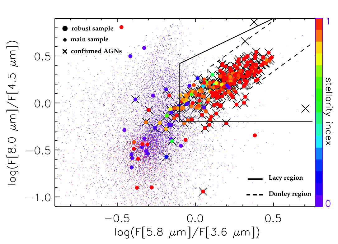
Figure 7: MIR diagram where colors are obtained as ratios of the fluxes in the four IRAC channels. Symbols are identical to Fig. 6. The solid lines delineate the region where AGNs are typically found according to Lacy et al. (2007), while the dashed lines define the less contaminated AGN region identified in Donley et al. (2012). A blob characterized by a high concentration of stars can be seen in the lower-left part of the diagram, while inactive galaxies tend to occupy the roughly vertical, scattered sequence defined by small violet dots.

5 Discussion

In this work we investigated the performance of optical variability as an AGN detection method, extending the monitoring baseline from the first five months already studied in De Cicco et al. (2015) up to three years, and the magnitude range 0.5 mag fainter. The larger baseline, coupled with the wealth of multiwavelength data available in the COSMOS field, allow significant improvements with respect to our previous investigations in COSMOS and the CDFS. In particular, we are able to select a robust sample of 299 AGN candidates, on the basis of their optical variability, and employ several multiwavelength diagnostics to confirm and characterize their nature. Table 2 collects and summarizes the results obtained by means of the various diagnostics described in the previous sections, while Table LABEL:tab:validation contains a detailed list of all the AGN candidates in our robust sample, with relevant information about them.

Table 2: Confirmed sources in the robust sample of AGN candidates. We include the number of sources confirmed by individual diagnostics (lines 3 to 6), as well as the number of sources (when not null) confirmed only by a specific combination of diagnostics, or by a single one of them (lines 7 to 14).

confirmed AGNs	256 (86% of 299)
confirmed stars	9 (3% of 299)
X/O validation (X)	248 (83% of 299)
spectroscopic validation (S)	225 (75% of 299)
Lacy region validation (L)	223 (75% of 299)
Donley region validation (D)	138 (46% of 299)
S+X+L+D validation	134
S+X+L validation	65
X+L+D validation	3
S+X validation	26
X+L validation	14
L+D validation	2
only X validation	6
only L validation	6
classified sources
with no X-ray counterpart	8

Here follows a list of our main findings, together with a comparison with the results from our previous analysis described in De Cicco et al. (2015).

1. We validate as AGNs 256 sources in the robust sample, yielding a purity of $86\%$ (256/299), and demonstrating the effectiveness of optical variability as an AGN selection method. This represents an improvement compared to the $81\%$ value we obtained in De Cicco et al. (2015), particularly considered the adoption of a more relaxed threshold (95% instead of the $3\sigma$ used in our previous work) and 0.5 magnitude fainter detection threshold. In Table LABEL:tab:validation we report the percentile each source belongs to; purer samples can be obtained by choosing more restrictive thresholds (e.g., 99th percentile).
   Regarding the contamination, our robust sample includes two sources which are spectroscopically classified as stars in the Chandra catalog; these two sources, together with seven additional X-ray undetected ones, lie on the stellar sequence in the diagram shown in Fig. 6. Among the seven stellar candidates with sufficient MIR color information to plot in Fig. 7, six fall within the expected stellar locus. Importantly, none of these sources are classified as AGNs by any of the diagnostics we used. As a consequence, we classify all nine of them as stars, implying a stellar contamination of $3\%$ (9/299). This leaves 34 sources in the robust sample with no classification. In the worst-case scenario where all of them are spurious, the contamination rate would be $14\%$. The 34 non-confirmed AGNs are mostly faint, only 10 of them having a magnitude r(AB) $<23$.

   In Section 3.3 we mentioned that the identification and analysis of SNe in VST-COSMOS data is currently ongoing (Ragosta et al., in prep.) but, at present, there are no identified SNe in our sample of AGN candidatates.

   We note that three of the 34 sources do not have a counterpart in any of the known COSMOS catalogs, even when we search for them using a larger matching radius than 1″. These sources were already part of our sample of AGN candidates in De Cicco et al. (2015, see Discussion there); they have average magnitudes $21.9<$ r(AB) $<22.4$, which is well above HST detection limit. Further investigation is necessary in order to unveil their nature.

   We point out that 11 sources belonging to the robust sample lie on the edges of the field, very close to the edge areas that we masked, or very close to other masked regions. Thus they are very likely to be spurious and we could have excluded them from our robust sample if we had enforced a stricter masking policy. We had already noticed these sources and their positions at the time we obtained the robust sample, but we chose not to exclude them a priori because we did not want to introduce a bias in the sample. Their exclusion would reduce the robust sample to 288 AGN candidates, yielding a potential confirmation of $89\%$ and contamination ranging from $3\%$ to $11\%$, depending on the nature of the unclassified sources. Three of the remaining 23 sources with no classification based on the used diagnostics are classified as stars in the COSMOS ACS catalog.

   If we consider that the analyzed sky area, not including masked regions, corresponds to $\approx 0.83$ sq. deg., the number of confirmed AGNs returns a density of $\approx 308$ AGNs per square degree.

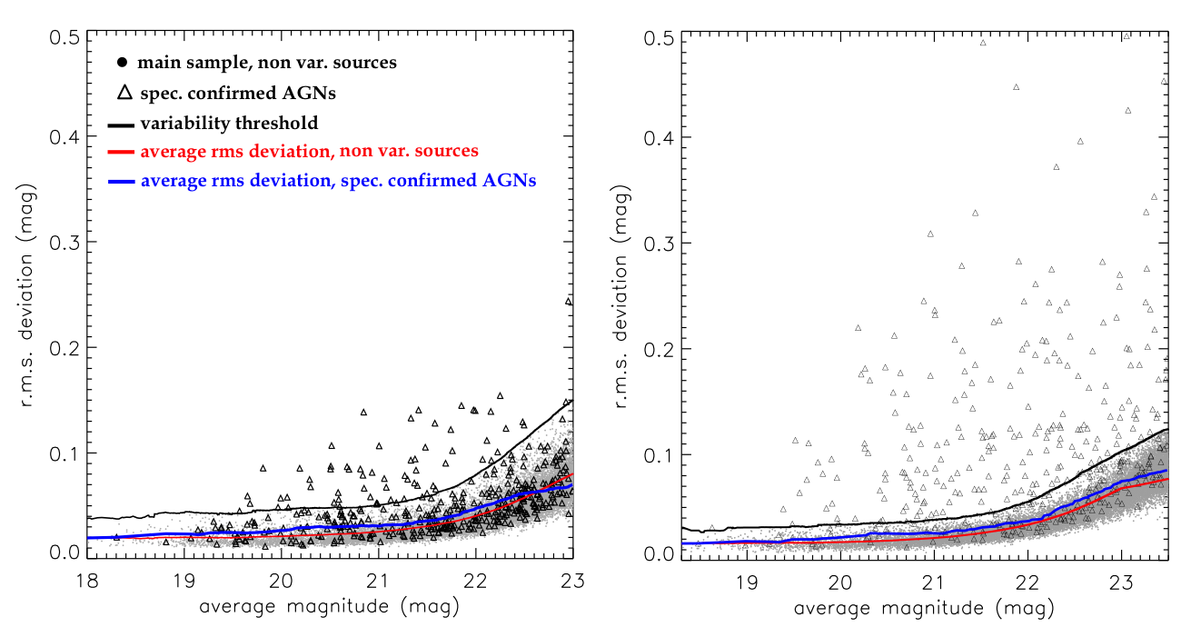
Figure 8: Light curve r.m.s. as a function of the average magnitude for all the non-variable sources in the main sample (small dots) and for those with an X-ray counterpart and that are spectroscopically confirmed to be AGNs (triangles), from our five month analysis (De Cicco et al. 2015, left panel) and the present analysis (right panel). In the left panel the vertical axis has been rescaled to the one in the right panel, while magnitudes are limited to r(AB) $\leq$ 23. The red and blue curves

2. We compute the completeness of AGNs in the robust sample with respect to the most reliable sample of AGNs available in COSMOS, i.e., sources with an X-ray counterpart and a spectroscopic classification as AGN; we obtain $59\%$ completeness. This percentage is remarkably higher than the $18\%$ completeness obtained in De Cicco et al. (2015). This means our result improved by a factor of 3.3. In Fig. 8 we show the improvement obtained in this work in the variability detection for X-ray AGNs compared to De Cicco et al. (2015), by reporting two diagrams showing the completeness for both our past and present analyses. In the five-month analysis (left panel) VST sources with an X-ray counterpart exhibited, on average, a higher variability than the whole sample of VST sources, although $>80\%$ of the sources with an X-ray counterpart fell below our variability threshold. At the time we predicted, based on the red-noise variability typical of AGNs, that a longer baseline would have returned a larger sample of sources above the variability threshold, and hence a much higher completeness (see Discussion and Fig. 8 in De Cicco et al. 2015); this is indeed what we found in the present analysis (right panel), where the completeness rises to 59% and the fraction of sources below the threshold hence drops from $>80\%$ to 41%.

   The completeness for unobscured AGNs is now 82%, while it is 18% for obscured ones. In De Cicco et al. (2015) we report a 25% and 6% completeness, respectively. We note that our past analysis was limited to sources with r(AB) $\leq 23$ mag, while here we go half a magnitude deeper. Anyway, we verified that the results are not affected by the different magnitude threshold, and would be the same if we adopted the same cut. This suggests that the improvement in the detection rate is an effect of the longer baseline, and Fig. 8 confirms that.

   The fraction of unobscured AGNs we retrieve is eight times larger than that of obscured ones. This is expected, since optical variability is biased towards the first class of AGNs, as we observe directly their inner regions (e.g., Padovani et al. 2017, and references therein).

   Taking the cue from what we did in De Cicco et al. (2015), we also computed the completeness in four magnitude bins, from r(AB) $=20$ to $23.5$ mag. We obtain 80%, 66%, and 53%, respectively, for the first three bins, which are one magnitude-sized. Similarly to De Cicco et al. (2015), these fractions are higher for brighter sources. The corresponding values in our previous work are 26%, 23%, and 5%. The remaining bin is half a magnitude-sized, and has no correspondance in our previous analysis; the completeness, in this case, is 45%.

   In Section 4.1 we mentioned that the completeness with respect to the AGNs confirmed by the X/O diagram is 37%. We note that the X-ray sample includes both unobscured and obscured AGNs, and that AGN selection based on optical variability is biased against the latter class. This is a possible explanation for the 37% completeness that we obtain.

3. In Section 3.3 we stated that our robust sample does not include 93 sources flagged 3 because of their doubtful variability. Based on the diagnostics we used throughout the present work, we would confirm as AGNs 12 of them. This number includes three sources confirmed only by the Lacy diagnostic which, as we mentioned in Section 4.3.2, is affected by non-AGN contamination; as a consequence, the number of sources labeled 3 and with a reliable confirmation of their AGN nature is 9/93 (10%), indicating that we are not biasing our results when removing sources affected by aesthetic or photometric problems.

In Fig. 9 we show a Venn diagram summarizing the main results obtained by the various diagnostics used to validate our sources. The sample selected by means of optical variability is largely in overlap with both X-ray and IR ones, yet partly complementary to both. This is due to our relatively bright limit and the approach adopted in this work, which selects bright quasar-like AGNs; other works show that addressing the problem of the host galaxy contamination through higher resolution instruments (e.g., Villforth et al. 2010; Sarajedini et al. 2011; Pouliasis et al. 2016, Pouliasis et al., in prep.) or through image subrtaction techniques (e.g., Botticella et al. 2017) allows recovering of complementary samples of low-luminosity or X-ray faint AGNs. In any case, variability allows to confirm AGN candidates identified by means of less robust/more contaminated diagnostics (e.g., Lacy et al. 2007).

The 256 confirmed AGNs were found analyzing data from 54 visits over a 3 yr baseline. In order to assess how the sampling cadence could affect the AGN detection efficiency of future surveys, we made some tests, varying the number of visits over a fixed baseline of 3.3 yr. When possible, we included visits from each of the three seasons, in order to obtain a coverage as homogeneous as possible. Consistent with what we did in the present work (see Section 3), we always required sources to be detected in at least half the visits. We show the results of this test in Fig. 10. The test shows how significantly a denser sampling affects the detection efficiency; this effect is often underestimated when planning monitoring campaigns as it is uncorrectly assumed that just increasing the baseline is sufficient to increase the number of detections, even if this means dramatically reducing the sampled cadence.

Sections 1 and 3 highlighted that the present work extends the analysis of De Cicco et al. (2015) to a longer baseline, and uses a different approach to correct magnitudes (reference visit vs. growth curves), select the sample of sources to include in the analysis (detection required in at least 50% vs. 20% of the visits), define a variability threshold (95th percentile vs. $3\sigma$ threshold). The present work also makes use of a $\sigma$-clipping algorithm when computing $\langle{\mbox{mag}}^{lc}\rangle$ and $\sigma^{lc}$ from the light curve of each source. It is thus worth comparing briefly the results obtained in our previous work with those we would obtain if we used this new approach in the analysis of the same dataset as in De Cicco et al. (2015), consisting of 27 visits over the first season of the VST survey of COSMOS.

In De Cicco et al. (2015) we obtained a sample of 83 AGN candidates (hereafter, sample 1), and confirmed as AGNs 67 (81%) of them. Following the new approach outlined in the present work, we would obtain a sample of 129 AGN candidates (hereafter, sample 2), and confirm as AGNs 101 (78%) of them, thus obtaining consistent results. In sample 2 we recover 84% of the AGN candidates and 90% of the confirmed AGNs in sample 1. The constraint on the number of detections does not significantly affect the result, since most of the sources in each of the inspected samples were detected in almost all the visits. We expect sample 2 to be larger than sample 1 due to the different threshold adopted, which now roughly corresponds to a $1.5\sigma$ threshold, rather than $3\sigma$. The $\sigma$-clipping algorithm, on the other side, reduces the inclusion of spurious sources in the sample of AGN candidates.

There is one major factor to take into account, i.e., the red-noise type variability of AGNs. Indeed, the complete analysis over the 3.3 yr baseline returns 99% of the confirmed AGNs from sample 1 and that do not fall in areas that in the new analysis we chose to mask. It also shows that there is only one AGN confirmed in sample 1 and not retrieved in the robust sample because it is below the variability threshold. All this proves that the adopted approach, coupled with the longer baseline, leads to improved results with respect to De Cicco et al. (2015), as also shown by the larger values obtained for purity and completeness.

In Section 2 we mentioned that so far our work has focused on $r$-band data; a complementary analysis of COSMOS $g$- and $i$-band variability, together with a multiband analysis combining $g$, $r$, and $i$ data, will be presented in a forthcoming paper. This will offer a chance to investigate correlated variability in different bands, together with the dependence of AGN variability on the specific wavelength range, and also average and time-dependent color selection (e.g., Richards et al. 2015); plus, the multiband analysis will retrieve more robust samples of candidates, simultaneously varying in multiple bands, thus minimizing contributions from contaminants.

represent the running average of the r.m.s. deviation for the two subsamples of sources, respectively. In the present work we find 59% of the sources in the second subsample above the variability threshold (black line), while they were only 15% in our former analysis.

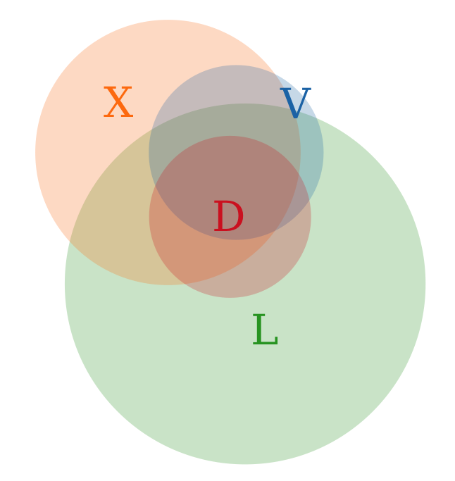
Figure 9: Venn diagram combining together the samples of AGNs selected by means of different diagnostics: optical variability (V), X-ray properties (X, from the X/O diagram), Lacy region (L), and Donley region (D). The circle sizes, as well as the overlap sizes, are quantitatively correct. The sample of optically variable sources includes the 34 sources that are not confirmed by any other diagnostics, while it does not include the nine sources confirmed as stars (see main text). It is apparent that the variability-selected sample largely overlaps both with the X-ray selected and the Lacy-selected AGNs, while the overlap with the Donley-selected sample is only partial.

Figure 10: Fraction of confirmed AGNs retrieved selecting an increasing number of visits over a fixed baseline of 3.3 yr, which corresponds to the baseline covered in the present work, and is the longest sampled timescale for VST-COSMOS data to date. Each point is the average result of 10 random simulations, the error bars being the corresponding thresholds for the 10th and the 90th percentiles. The plot shows that, as the number of visits increases, we are able to retrieve a larger fraction of AGNs. A denser sampling leads to a reduction in the size of the error bars, as an effect of the reduced differences among the possible patterns that can be chosen for the simulation.

Table 3: List of the 299 optically variable sources in the robust sample. Column meanings: (1): identification number; (2) and (3): right ascension and declination (J2000); (4): average VST r(AB) magnitude; (5): r.m.s. of the light curve; (6): SExtractor stellarity index; (7): quality label; (8): percentile: the number indicates that the $\sigma^{lc}$ of the source is above the threshold of the corresponding percentile; (9): redshift: mostly spectroscopic redshifts from Marchesi et al. (2016); when not available, spectroscopic redshift from Hasinger et al. (2018), marked by a star; or spectroscopic redshift from Lilly et al. (2007, box); or photometric redshift from Marchesi et al. (2016, diamond); or photometric redshift from Ilbert et al. (2009, triangle); (10): number of visits where the source is detected; (11): source classification. The classification index is the sum of different numbers corresponding to the following key: 1 = confirmed AGN through spectroscopy/SED; 2=confirmed AGN through X/O diagram; 4 = confirmed AGN through IRAC color diagram, Lacy region; 8 = confirmed AGN through IRAC color diagram, Donley region; 0 = non-classified; -1 = star.

source ID	RA J2000 (deg)	Dec J2000 (deg)	avg $r(AB)$ mag (mag)	ltc r.m.s. (mag)	stellarity	quality label	percentile	redshift	# of detections	classification
(1)	(2)	(3)	(4)	(5)	(6)	(7)	(8)	(9)	(10)	(11)
1	149.68732	1.7191443	20.26	0.11	0.90	1	99	1.35	54	15
2	150.07553	1.7199465	23.23	0.11	0.36	2	95	0.868$\triangle$	46	0
3	149.99166	1.7243215	20.68	0.11	0.93	1	98	1.625	52	15
4	149.84359	1.7331874	23.36	0.12	0.97	2	95	0.059$\triangle$	47	0
5	150.39678	1.7357309	22.47	0.11	0.97	1	98	2.766	54	15
6	150.12141	1.7397895	23.49	0.13	0.01	1	96	0.723$\triangle$	36	0
7	150.27996	1.7438591	23.08	0.20	0.43	2	99	0.763	51	3
8	150.05048	1.7444366	22.20	0.21	0.72	1	99	1.149	52	7
9	149.77079	1.7466641	21.53	0.14	0.92	2	99	1.327	54	2
10	149.64483	1.7506337	19.52	0.11	0.87	1	99	1.9	54	15
11	150.21676	1.7511995	20.03	0.04	0.03	2	96	0.1679$\Box$	54	0
12	150.26242	1.7515061	23.27	0.28	0.85	1	99	1.676	44	15
13	150.25924	1.7573333	22.71	0.17	0.02	2	99	0.965	54	6
14	150.10740	1.7592058	22.73	0.11	0.98	1	98	3.949	51	2
15	150.17663	1.7595157	22.20	0.12	0.83	1	99	1.161	54	15
16	150.53564	1.7649016	21.81	0.17	0.94	1	99	2.204	54	15
17	150.49173	1.7725595	21.86	0.06	0.16	1	97	0.833	54	7
18	150.48517	1.7836715	22.92	0.11	0.98	1	97	2.727$\triangle$	53	14
19	150.22784	1.7869356	23.07	0.11	0.31	1	95	1.681	52	7
20	150.59603	1.7874690	21.52	0.12	0.89	1	99	1.246	54	15
21	150.19511	1.7938135	22.98	0.27	0.51	1	99	1.867	54	15
22	150.13174	1.7993850	21.10	0.07	0.93	1	98	1.679	52	15
23	150.48525	1.8030591	22.56	0.12	0.85	1	99	0.957	54	15
24	149.83469	1.8176868	22.80	0.22	0.98	1	99	0.735	50	15
25	150.36590	1.8292915	21.82	0.38	0.91	1	99	0.958	54	6
26	149.82193	1.8386822	21.22	0.21	0.93	1	99	1.351	52	15
27	149.81686	1.8467454	21.03	0.08	0.95	1	98	1.035	53	7
28	149.76952	1.8495966	22.98	0.26	0.90	1	99	2.242	52	7
29	150.06795	1.8513342	21.29	0.12	0.89	2	99	1.134	52	7
30	150.04684	1.8667762	22.00	0.15	0.97	1	99	2.412	52	7
31	150.24309	1.8692006	20.89	0.06	0.91	1	97	2.021	53	15
32	150.20827	1.8754041	20.64	0.18	0.91	1	99	1.147	54	15
33	150.13916	1.8769595	20.81	0.06	0.90	1	97	0.831	54	15
34	150.02547	1.8777086	23.10	0.18	0.93	1	99	1.796	51	7
35	150.16181	1.8779243	22.41	0.24	0.98	1	99	1.444	54	15
36	149.67421	1.8883298	20.43	0.04	0.89	1	95	1.784	54	15
37	150.24520	1.9001845	20.19	0.22	0.91	1	99	1.56	50	15
38	150.49135	1.9102721	22.34	0.11	0.97	1	98	2.234	51	15
39	150.40095	1.9119384	21.47	0.07	0.95	1	98	2.279	51	15
40	150.30891	1.9123230	22.43	0.31	0.88	1	99	1.483$\diamond$	52	6
41	150.22938	1.9219723	23.48	0.13	0.01	2	96	0.543$\triangle$	29	0
42	150.53943	1.9236345	20.63	0.05	0.03	1	97	-	51	4
43	150.58125	1.9269990	19.90	0.10	0.86	1	98	1.513	51	7
44	150.32725	1.9286116	20.88	0.07	0.03	1	98	0.528	51	15
45	150.11702	1.9298758	22.69	0.20	0.75	2	99	1.519	51	7
46	149.98871	1.9324447	22.65	0.16	0.99	1	99	2.406	51	15
47	150.43103	1.9352358	21.69	0.23	0.98	1	99	2.177	51	15
48	150.35943	1.9364083	22.81	0.15	0.97	1	99	2.377	51	15
49	150.22042	1.9539866	21.06	0.04	0.95	2	96	0.0	52	-1
50	149.67661	1.9563377	19.35	0.03	0.91	1	95	0.0$\triangle$	54	-1
51	150.27892	1.9595724	21.32	0.16	0.90	1	99	1.55	52	3
52	150.35308	1.9607742	21.63	0.11	0.95	1	98	1.173	52	15
53	150.25323	1.9661424	21.40	0.05	0.05	1	97	0.4263$\Box$	51	4
54	150.38668	1.9665945	21.40	0.17	0.90	1	99	1.537	50	15
55	150.44890	1.9767770	23.32	0.12	0.18	2	95	0.834$\triangle$	45	0
56	150.57489	1.9767948	21.37	0.09	0.92	1	98	1.541	50	15
57	150.31189	1.9779708	22.63	0.62	0.94	1	99	2.347	50	15
58	149.92257	1.9792039	22.35	0.13	0.98	1	99	2.503	52	15
59	149.63091	1.9794908	23.29	0.12	0.00	2	96	0.9989$\Box$	35	0
60	149.67516	1.9827144	21.60	0.17	0.96	1	99	1.334	54	15
61	149.77965	1.9843906	23.40	0.12	0.02	2	96	0.206$\triangle$	41	0
62	150.46193	1.9846376	23.15	0.12	0.01	2	96	0.135$\triangle$	42	0
63	150.21635	1.9887359	21.56	0.12	0.97	1	99	2.231	52	15
64	150.15819	1.9911670	23.46	0.13	0.01	2	97	1.195$\triangle$	31	4
65	150.25342	1.9966557	21.99	0.21	0.90	1	99	1.171	50	7
66	149.95772	2.0030978	21.27	0.06	0.94	1	98	1.806	51	15
67	150.07306	2.0035314	21.25	0.08	0.26	1	98	0.352	54	7
68	150.19559	2.0044371	20.22	0.18	0.90	1	99	1.923	52	15
69	150.50321	2.0047865	23.40	0.12	0.03	1	95	0.6606$\Box$	32	0
70	149.99524	2.0066641	22.35	0.12	0.97	1	98	1.033	52	7
71	150.46299	2.0090191	20.56	0.16	0.90	1	99	0.967	52	15
72	150.42255	2.0141421	22.15	0.21	0.91	1	99	2.283	51	15
73	150.28566	2.0146151	21.32	0.18	0.93	1	99	2.671	51	15
74	150.05892	2.0151912	19.97	0.03	0.87	1	95	2.498	54	15
75	149.81419	2.0163414	23.05	0.50	0.97	1	99	1.36	54	7
76	149.71559	2.0165170	22.95	0.23	0.98	1	99	2.686	52	3
77	149.95585	2.0280685	19.48	0.03	0.98	1	96	1.753	52	15
78	149.88699	2.0336446	23.46	0.16	0.23	1	99	-	48	0
79	150.31195	2.0357509	21.58	0.08	0.63	1	98	0.971	51	3
80	150.19448	2.0425058	20.13	0.05	0.88	1	97	0.0	53	-1
81	150.14566	2.0430791	20.91	0.08	0.91	1	98	1.178	53	15
82	150.44603	2.0435056	21.13	0.11	0.91	1	98	1.171	51	7
83	149.89512	2.0472080	22.21	0.12	0.98	1	99	2.198	51	15
84	150.44369	2.0491068	20.42	0.07	0.89	1	97	0.669	51	15
85	149.65632	2.0511320	23.48	0.18	0.89	1	99	1.854	48	7
86	150.53574	2.0577803	22.09	0.07	0.97	1	97	1.195	51	3
87	150.33439	2.0614565	20.26	0.11	0.88	1	98	0.904	52	15
88	150.45768	2.0624709	21.58	0.10	0.98	1	98	2.325	51	15
89	150.19474	2.0679277	20.48	0.08	0.03	1	98	0.552	53	15
90	149.91055	2.0679895	23.28	0.20	0.97	1	99	1.091	50	15
91	149.79440	2.0731069	23.33	0.14	0.98	1	99	2.668	52	15
92	149.66920	2.0740675	20.15	0.04	0.03	1	96	0.34	54	7
93	150.40639	2.0756581	23.05	0.20	0.89	1	99	1.257	49	7
94	149.73378	2.0763561	22.98	0.14	0.96	2	99	2.042	49	7
95	149.90957	2.0805839	20.74	0.10	0.90	1	98	2.802	52	15
96	150.20798	2.0833580	19.76	0.09	0.87	1	98	1.236	53	15
97	150.41830	2.0851684	20.82	0.04	0.03	2	96	0.424	51	7
98	149.66359	2.0852282	20.47	0.06	0.89	1	97	1.22	54	7
99	150.12289	2.0858446	23.50	0.14	0.03	2	98	0.6606$\Box$	45	0
100	150.32426	2.0890822	23.31	0.24	0.99	1	99	1.797	50	3
101	149.82267	2.0896669	22.45	0.21	0.91	1	99	2.051	54	7
102	150.12558	2.0907611	23.22	0.12	0.98	2	96	0.0$\triangle$	52	0
103	149.89795	2.0939249	22.28	0.20	0.98	1	99	1.921	51	15
104	150.10203	2.1054810	19.85	0.05	0.86	2	98	2.288	54	15
105	150.22434	2.1056295	21.51	0.10	0.04	2	98	0.74	52	3
106	150.55902	2.1057491	22.83	0.17	0.97	1	99	2.323	50	15
107	150.59573	2.1111357	22.02	0.10	0.94	2	98	0.899	51	15
108	150.37361	2.1120309	20.85	0.13	0.95	1	99	1.914	51	15
109	150.42092	2.1124419	23.27	0.19	0.78	1	99	1.263	49	6
110	150.29241	2.1137305	22.95	0.11	0.87	1	97	1.828	53	7
111	150.26170	2.1166520	21.43	0.07	0.98	1	98	2.572	52	15
112	149.93092	2.1187187	19.66	0.11	0.88	1	99	2.194	54	15
113	150.32828	2.1249531	22.25	0.12	0.95	1	99	1.774	52	7
114	150.10559	2.1263062	21.96	0.24	0.95	1	99	0.961	54	15
115	149.85448	2.1324290	23.03	0.11	0.30	1	97	0.955	50	2
116	150.19901	2.1325192	19.81	0.08	0.89	1	98	2.159	54	15
117	150.15847	2.1395817	20.70	0.08	0.92	1	98	1.826	54	15
118	150.43540	2.1428146	22.88	0.14	0.03	1	99	0.968	51	7
119	150.45186	2.1448420	20.89	0.25	0.91	1	99	1.298	51	15
120	149.71124	2.1451715	20.73	0.13	0.90	1	99	1.53	54	15
121	150.34592	2.1475287	20.91	0.04	0.91	1	95	1.256	54	7
122	150.29726	2.1488036	20.97	0.04	0.92	1	96	3.328	53	15
123	150.10874	2.1569871	23.40	0.17	0.96	2	99	1.814	44	7
124	150.30261	2.1610864	20.70	0.05	0.90	1	97	1.817	53	15
125	150.48442	2.1620498	22.34	0.19	0.98	1	99	1.639	53	7
126	149.82791	2.1643113	20.48	0.08	0.89	1	98	1.156	52	15
127	150.47551	2.1710079	23.46	0.12	0.00	2	95	1.269*	33	0
128	149.89485	2.1744358	22.08	0.26	0.97	1	99	1.312	54	7
129	150.42224	2.1754161	21.44	0.33	0.88	2	99	0.979	54	15
130	150.57633	2.1813797	20.88	0.05	0.03	1	97	0.554	53	3
131	150.53190	2.1888941	21.78	0.09	0.97	1	98	0.827	52	15
132	150.19984	2.1908592	21.22	0.06	0.92	1	98	1.515	54	15
133	150.37825	2.1964202	23.26	0.33	0.63	1	99	1.512	50	7
134	149.91246	2.2003194	20.75	0.07	0.91	1	98	0.686	54	15
135	150.04599	2.2011612	22.32	0.09	0.91	2	98	2.704	54	7
136	150.21473	2.2042706	21.22	0.15	0.93	1	99	1.841	54	15
137	150.13410	2.2045658	23.50	0.13	0.17	1	96	0.67$\triangle$	32	0
138	150.08603	2.2097157	21.78	0.10	0.07	2	98	0.2386$\Box$	54	0
139	150.02856	2.2099369	21.44	0.18	0.92	1	99	1.258	53	15
140	150.42124	2.2166694	22.06	0.06	0.90	1	96	0.621	54	7
141	149.73895	2.2206892	20.68	0.08	0.91	1	98	1.024	49	15
142	150.58111	2.2210492	22.31	0.08	0.98	1	97	2.022	52	15
143	149.87918	2.2258118	22.74	0.11	0.92	2	98	3.65	51	3
144	149.82359	2.2282771	22.62	0.11	0.98	1	98	2.97	49	7
145	150.27216	2.2300959	20.96	0.17	0.92	1	99	2.611	54	15
146	150.00447	2.2370960	22.20	0.10	0.56	1	98	1.406	51	15
147	150.09361	2.2372209	23.01	0.14	0.09	1	99	1.4373$\Box$	51	4
148	149.89539	2.2394848	21.09	0.05	0.93	1	97	1.729	52	15
149	150.34994	2.2461224	21.29	0.28	0.90	1	99	0.894	54	7
150	150.44961	2.2464424	20.78	0.12	0.91	1	99	0.882	54	15
151	149.74392	2.2497706	18.63	0.03	0.03	2	97	0.133	48	3
152	150.47956	2.2531361	22.45	0.08	0.95	1	96	0.866	54	6
153	149.82193	2.2546519	22.27	0.13	0.03	2	99	0.934	47	3
154	150.01053	2.2559001	23.30	0.12	0.97	1	96	1.661	49	7
155	149.77136	2.2583635	21.91	0.12	0.93	2	99	2.213	47	15
156	149.99364	2.2585206	21.51	0.12	0.04	2	99	0.658	51	7
157	150.01822	2.2594497	23.21	0.12	0.98	1	96	2.673	50	15
158	150.42609	2.2600481	23.16	0.12	0.00	1	98	0.814*	46	0
159	150.49208	2.2634375	23.50	0.16	0.96	2	99	0.835$\triangle$	48	0
160	150.39264	2.2701100	23.38	0.14	0.96	1	98	2.158	49	7
161	150.53616	2.2732704	21.77	0.08	0.57	1	98	1.081	54	7
162	150.32195	2.2744886	22.31	0.13	0.88	2	99	0.3517$\Box$	54	4
163	150.00927	2.2755091	20.58	0.14	0.85	2	99	0.85	52	15
164	149.85155	2.2764230	23.37	0.13	0.98	2	98	3.372	44	3
165	149.70633	2.2779600	21.61	0.12	0.19	1	99	0.731	54	7
166	149.66680	2.2864436	21.88	0.45	0.92	1	99	1.028	54	7
167	150.58184	2.2877456	21.81	0.12	0.96	1	99	1.343	54	15
168	149.63869	2.2890013	20.72	0.09	0.94	1	98	0.231$\triangle$	54	12
169	150.23628	2.2891123	21.58	0.11	0.96	1	98	2.076	54	15
170	150.08439	2.2904945	22.80	0.28	0.87	1	99	2.101	51	7
171	150.13800	2.2916745	19.80	0.04	0.03	2	96	0.185	52	2
172	149.71529	2.2994018	23.49	0.19	0.97	1	99	1.191	46	7
173	149.99392	2.3014085	20.29	0.10	0.88	1	98	1.796	51	15
174	150.36670	2.3053423	21.94	0.20	0.98	1	99	1.187	54	7
175	149.86340	2.3060702	23.45	0.13	0.98	2	97	0.74$\triangle$	44	-1
176	149.91975	2.3274421	20.82	0.09	0.91	1	98	1.454	51	15
177	150.06456	2.3290367	22.42	0.18	0.98	1	99	2.45	52	15
178	149.86802	2.3306993	20.70	0.15	0.90	1	99	1.478	49	7
179	149.76351	2.3341496	21.41	0.14	0.93	1	99	1.137	47	15
180	149.79165	2.3382080	21.93	0.07	0.87	1	97	1.008	49	3
181	149.95514	2.3402663	19.65	0.03	0.87	1	96	0.01$\triangle$	52	-1
182	150.35361	2.3421398	20.74	0.07	0.94	1	98	1.708	54	15
183	149.84949	2.3431028	23.10	0.25	0.98	2	99	0.792	48	14
184	149.91949	2.3453929	21.85	0.12	0.91	1	99	3.015	51	15
185	149.81295	2.3454732	22.26	0.07	0.93	2	96	1.812	48	7
186	149.88329	2.3467476	21.94	0.09	0.92	1	98	1.021	51	7
187	149.65292	2.3469199	23.07	0.43	0.97	1	99	1.188	54	7
188	149.67864	2.3489133	23.47	0.17	0.91	1	99	2.017	45	7
189	149.72076	2.3489995	22.73	0.20	0.94	1	99	1.53	52	6
190	149.86798	2.3518587	20.45	0.04	0.03	2	96	0.346	51	7
191	150.25560	2.3534942	23.03	0.25	0.94	1	99	2.975$\diamond$	52	6
192	150.02012	2.3536062	22.06	0.08	0.98	1	98	2.663$\diamond$	52	14
193	149.95061	2.3545852	23.16	0.36	0.15	1	99	0.919$\triangle$	49	0
194	150.12366	2.3582506	21.01	0.09	0.05	1	98	0.728	52	7
195	150.23181	2.3639768	21.18	0.08	0.94	1	98	1.936	54	15
196	150.40667	2.3654220	22.25	0.28	0.98	1	99	2.032	54	15
197	149.73882	2.3663495	23.00	0.14	0.93	2	99	1.65	47	3
198	149.94552	2.3692673	21.52	0.49	0.94	1	99	0.909	52	15
199	150.44442	2.3697490	22.20	0.19	0.44	1	99	0.891	54	7
200	149.84814	2.3742413	21.01	0.23	0.96	1	99	2.735	48	15
201	149.83285	2.3846825	22.34	0.24	0.98	1	99	2.247	47	15
202	150.52679	2.3846957	22.97	0.12	0.86	1	98	1.299	52	3
203	149.91690	2.3851880	19.96	0.08	0.88	1	98	1.131	52	15
204	150.42194	2.3854774	23.26	0.24	0.98	1	99	1.514	46	3
205	150.45038	2.3880675	23.42	0.20	0.97	1	99	1.075$\diamond$	45	6
206	150.21076	2.3914776	22.85	0.10	0.60	1	96	3.095	51	15
207	150.45848	2.3973237	22.20	0.08	0.86	2	98	2.89	54	15
208	150.09155	2.3990645	22.37	0.14	0.99	1	99	2.47	52	15
209	150.17396	2.4030030	23.16	0.14	0.43	1	99	0.979	46	15
210	150.51163	2.4096278	21.03	0.11	0.92	1	98	0.986	54	15
211	150.47206	2.4102167	20.85	0.11	0.79	1	98	0.668	54	15
212	149.85622	2.4104209	20.78	0.04	0.94	2	95	0.0$\triangle$	46	-1
213	149.66026	2.4109485	22.60	0.13	0.10	1	99	1.161	53	15
214	150.49569	2.4125739	21.75	0.08	0.87	1	98	1.369	54	15
215	150.43815	2.4157843	20.80	0.06	0.91	1	97	2.02	54	15
216	149.87067	2.4172606	22.54	0.12	0.98	2	99	1.528	50	15
217	149.76069	2.4198974	22.08	0.12	0.94	1	99	1.101	50	3
218	150.42437	2.4220652	18.51	0.03	0.03	1	95	-	54	0
219	150.38663	2.4223974	21.05	0.04	0.97	1	95	-	54	0
220	150.54404	2.4230778	23.19	0.18	0.01	1	99	0.957	46	3
221	150.51395	2.4233098	20.08	0.03	0.96	1	95	-	54	-1
222	150.12409	2.4313257	22.98	0.11	0.00	2	96	0.757*	32	0
223	150.20898	2.4384817	21.60	0.05	0.96	1	95	3.715	52	15
224	149.93588	2.4405710	22.34	0.13	0.87	1	99	0.993	54	15
225	149.77695	2.4442782	23.12	0.12	0.97	2	98	4.171	50	3
226	150.49916	2.4449390	19.56	0.06	0.88	1	98	2.03	54	15
227	150.06217	2.4550396	21.53	0.07	0.14	1	98	0.73	52	7
228	149.72048	2.4587871	23.47	0.16	0.59	2	99	-	45	0
229	150.32742	2.4608443	20.66	0.08	0.62	1	98	1.042	54	15
230	150.03588	2.4645999	23.29	0.12	0.98	2	95	-	50	0
231	149.75093	2.4699039	21.16	0.06	0.51	2	97	0.658	51	7
232	150.00452	2.4765675	20.20	0.03	0.98	1	95	0.0$\triangle$	54	-1
233	150.10669	2.4772543	22.03	0.06	0.98	1	96	0.0$\triangle$	52	-1
234	150.05872	2.4774000	20.48	0.18	0.91	1	99	1.258	54	15
235	150.42870	2.4782022	23.21	0.11	0.02	2	95	0.168$\triangle$	45	12
236	150.40702	2.4788544	21.92	0.18	0.32	1	99	0.367	53	15
237	150.20884	2.4819287	19.96	0.04	0.87	1	97	3.333	52	15
238	149.97694	2.4866390	23.08	0.15	0.93	1	99	2.089	51	15
239	149.99068	2.4990856	23.39	0.12	0.80	2	95	2.022$\triangle$	32	0
240	150.37096	2.5001018	23.44	0.13	0.98	2	96	0.0$\triangle$	39	0
241	149.95562	2.5020388	22.54	0.17	0.96	1	99	1.458	53	7
242	150.39866	2.5028107	23.41	0.13	0.02	2	96	-	32	0
243	150.56735	2.5035958	21.50	0.06	0.92	1	97	1.146	54	15
244	149.93839	2.5059488	22.58	0.08	0.00	2	95	0.893	53	3
245	150.54475	2.5072799	19.39	0.05	0.90	1	98	1.16	54	15
246	149.92025	2.5142271	22.68	0.09	0.96	1	96	0.698	53	3
247	150.45062	2.5173912	21.93	0.13	0.96	1	99	-	51	0
248	150.60068	2.5188092	22.63	0.12	0.42	1	99	0.669	53	3
249	150.51820	2.5217408	22.92	0.13	0.77	1	99	2.779	53	15
250	150.41591	2.5257835	22.57	0.10	0.98	1	98	1.444	53	3
251	150.45356	2.5279411	21.26	0.13	0.91	1	99	1.935	54	15
252	150.56357	2.5361171	22.46	0.10	0.02	2	98	0.496$\triangle$	53	0
253	150.53936	2.5420789	22.50	0.10	0.97	1	98	1.716	52	7
254	150.38608	2.5426687	22.41	0.14	0.87	2	99	-	52	0
255	149.86034	2.5447442	23.35	0.22	0.98	1	99	1.596	51	15
256	149.69586	2.5490825	22.77	0.10	0.14	2	96	1.776	41	7
257	149.94219	2.5522457	23.44	0.12	0.00	2	95	0.6683$\Box$	28	0
258	149.91067	2.5546511	20.85	0.05	0.65	1	97	0.753	54	7
259	149.78568	2.5547887	23.13	0.14	0.93	1	99	1.798	52	7
260	149.81148	2.5579622	23.35	0.34	0.72	1	99	2.152	47	7
261	149.79633	2.5594275	22.72	0.11	0.96	1	98	1.541	52	15
262	150.38282	2.5597507	23.45	0.45	0.48	1	99	2.066	33	15
263	150.33449	2.5614370	20.26	0.18	0.88	1	99	1.836	54	15
264	149.79622	2.5641002	21.02	0.04	0.91	1	96	0.704	53	15
265	150.55593	2.5643882	22.35	0.09	0.97	1	98	1.143	54	15
266	149.77797	2.5672597	22.09	0.18	0.79	2	99	0.72	54	6
267	149.70362	2.5781197	21.00	0.24	0.89	1	99	1.545	54	15
268	150.23084	2.5782007	19.64	0.08	0.86	1	99	1.402	51	15
269	150.60793	2.5950421	23.25	0.12	0.00	2	95	0.627	42	0
270	150.16382	2.5977140	22.23	0.24	0.96	1	99	1.589	51	15
271	149.63532	2.5988504	22.02	0.06	0.83	1	97	2.536	53	15
272	149.65574	2.6008206	21.63	0.12	0.03	1	99	0.735	54	15
273	150.31792	2.6020259	21.30	0.20	0.56	1	99	0.958	54	15
274	150.47164	2.6032998	22.01	0.11	0.70	2	98	-	52	0
275	150.54274	2.6059349	22.29	0.26	0.77	1	99	0.98	54	6
276	149.85475	2.6069132	22.96	0.51	0.89	1	99	2.111$\diamond$	46	6
277	149.73649	2.6107833	22.12	0.13	0.27	2	99	1.324	53	7
278	150.59743	2.6179205	21.90	0.28	0.87	1	99	1.447	54	7
279	150.59193	2.6193782	23.09	0.12	0.94	1	98	2.994$\triangle$	53	4
280	150.12688	2.6265730	22.56	0.40	0.77	1	99	1.837	53	7
281	150.04250	2.6291486	21.07	0.10	0.90	2	98	1.569	54	3
282	150.04189	2.6294252	22.51	0.13	0.37	2	99	-	54	2
283	150.10281	2.6302075	22.54	0.08	0.04	2	95	1.182	53	3
284	150.09495	2.6338103	23.30	0.17	0.94	1	99	1.183	51	2
285	150.08056	2.6345305	22.42	0.08	0.98	1	95	0.71	53	15
286	150.55491	2.6410387	21.97	0.08	0.38	1	98	1.142	54	15
287	150.03431	2.6411103	22.05	0.07	0.04	1	97	0.518	54	15
288	149.80802	2.6456649	21.63	0.23	0.90	1	99	2.082	54	7
289	150.45662	2.6481900	20.67	0.05	0.87	1	97	2.05	54	15
290	150.49762	2.6599360	20.31	0.17	0.88	1	99	0.854	54	15
291	149.88379	2.6664010	22.54	0.08	0.66	1	95	1.346	54	6
292	150.29776	2.6734549	22.16	0.20	0.91	1	99	1.593	54	6
293	150.59885	2.6743665	20.81	0.04	0.02	2	95	0.066$\triangle$	54	0
294	150.50550	2.6749128	21.79	0.27	0.97	1	99	1.289	54	6
295	150.35149	2.6781381	20.96	0.31	0.85	1	99	2.754	54	15
296	150.03067	2.6787261	22.30	0.37	0.92	1	99	1.951	54	7
297	149.92542	2.6842236	20.57	0.21	0.90	1	99	1.779	53	3
298	150.04527	2.6884792	22.08	0.19	0.98	1	99	1.436	54	7
299	149.87593	2.6902237	21.78	0.06	0.87	1	97	2.169	54	15

Table 3: Continued.

References

- Alexander et al. (2002) Alexander, D. M., Vignali, C., Bauer, F. E., et al. 2002, AJ, 123, 1149
- Bertin & Arnouts (1996) Bertin, E. & Arnouts, S. 1996, A&AS, 117, 393
- Botticella et al. (2017) Botticella, M. T., Cappellaro, E., Greggio, L., et al. 2017, A&A, 598, A50
- Botticella et al. (2013) Botticella, M. T., Cappellaro, E., Pignata, G., et al. 2013, The Messenger, 151, 29
- Boutsia et al. (2009) Boutsia, K., Leibundgut, B., Trevese, D., & Vagnetti, F. 2009, A&A, 497, 81
- Brandt & Alexander (2015) Brandt, W. N. & Alexander, D. M. 2015, A&A Rev., 23, 1
- Brandt & Hasinger (2005) Brandt, W. N. & Hasinger, G. 2005, ARA&A, 43, 827
- Brandt et al. (2018) Brandt, W. N., Ni, Q., Yang, G., et al. 2018, arXiv e-prints 1811.06542
- Brusa et al. (2010) Brusa, M., Civano, F., Comastri, A., et al. 2010, ApJ, 716, 348
- Capaccioli & Schipani (2011) Capaccioli, M. & Schipani, P. 2011, The Messenger, 146, 2
- Capaccioli et al. (2015) Capaccioli, M., Spavone, M., Grado, A., et al. 2015, A&A, 581, A10
- Capak et al. (2007) Capak, P., Aussel, H., Ajiki, M., et al. 2007, ApJS, 172, 99
- Chiaraluce et al. (2018) Chiaraluce, E., Vagnetti, F., Tombesi, F., & Paolillo, M. 2018, A&A, 619, A95
- Choi et al. (2014) Choi, Y., Gibson, R. R., Becker, A. C., et al. 2014, ApJ, 782, 37
- Civano et al. (2012) Civano, F., Elvis, M., Brusa, M., et al. 2012, ApJS, 201, 30
- Civano et al. (2016) Civano, F., Marchesi, S., Comastri, A., et al. 2016, ApJ, 819, 62
- De Cicco et al. (2015) De Cicco, D., Paolillo, M., Covone, G., et al. 2015, A&A, 574, A112
- Donley et al. (2012) Donley, J. L., Koekemoer, A. M., Brusa, M., et al. 2012, ApJ, 748, 142
- Falocco et al. (2015) Falocco, S., Paolillo, M., Covone, G., et al. 2015, A&A, 579, A115
- Fazio et al. (2004) Fazio, G. G., Hora, J. L., Allen, L. E., et al. 2004, ApJS, 154, 10
- Ferrarese & Merritt (2000) Ferrarese, L. & Merritt, D. 2000, ApJ, 539, L9
- Gaskell & Klimek (2003) Gaskell, C. M. & Klimek, E. S. 2003, Astronomical and Astrophysical Transactions, 22, 661
- Grado et al. (2012) Grado, A., Capaccioli, M., Limatola, L., & Getman, F. 2012, Memorie della Societa Astronomica Italiana Supplementi, 19, 362
- Graham et al. (2014) Graham, M. J., Djorgovski, S. G., Drake, A. J., et al. 2014, MNRAS, 439, 703
- Hasinger et al. (2018) Hasinger, G., Capak, P., Salvato, M., et al. 2018, ApJ, 858, 77
- Huang et al. (2011) Huang, Z., Radovich, M., Grado, A., et al. 2011, A&A, 529, A93
- Ilbert et al. (2009) Ilbert, O., Capak, P., Salvato, M., et al. 2009, ApJ, 690, 1236
- Klesman & Sarajedini (2007) Klesman, A. & Sarajedini, V. 2007, ApJ, 665, 225
- Koekemoer et al. (2007) Koekemoer, A. M., Aussel, H., Calzetti, D., et al. 2007, ApJS, 172, 196
- Kuijken (2011) Kuijken, K. 2011, The Messenger, 146, 8
- Lacy et al. (2007) Lacy, M., Petric, A. O., Sajina, A., et al. 2007, AJ, 133, 186
- Lacy et al. (2004) Lacy, M., Storrie-Lombardi, L. J., Sajina, A., et al. 2004, ApJS, 154, 166
- Laigle et al. (2016) Laigle, C., McCracken, H. J., Ilbert, O., et al. 2016, ApJS, 224, 24
- Lilly et al. (2007) Lilly, S. J., Le Fèvre, O., Renzini, A., et al. 2007, ApJS, 172, 70
- Lintott et al. (2009) Lintott, C. J., Schawinski, K., Keel, W., et al. 2009, MNRAS, 399, 129
- LSST Science Collaboration et al. (2009) LSST Science Collaboration, Abell, P. A., Allison, J., et al. 2009, ArXiv e-prints 0912.0201
- Maccacaro et al. (1988) Maccacaro, T., Gioia, I. M., Wolter, A., Zamorani, G., & Stocke, J. T. 1988, ApJ, 326, 680
- MacLeod et al. (2011) MacLeod, C. L., Brooks, K., Ivezić, Ž., et al. 2011, ApJ, 728, 26
- Magorrian et al. (1998) Magorrian, J., Tremaine, S., Richstone, D., et al. 1998, AJ, 115, 2285
- Mainieri et al. (2002) Mainieri, V., Bergeron, J., Hasinger, G., et al. 2002, A&A, 393, 425
- Marchesi et al. (2016) Marchesi, S., Civano, F., Elvis, M., et al. 2016, ApJ, 817, 34
- McCracken et al. (2010) McCracken, H. J., Capak, P., Salvato, M., et al. 2010, ApJ, 708, 202
- Mushotzky (2004) Mushotzky, R. 2004, in Astrophysics and Space Science Library, Vol. 308, Supermassive Black Holes in the Distant Universe, ed. A. J. Barger, 53
- Nakos et al. (2009) Nakos, T., Willis, J. P., Andreon, S., et al. 2009, A&A, 494, 579
- Padovani et al. (2017) Padovani, P., Alexander, D. M., Assef, R. J., et al. 2017, A&A Rev., 25, 2
- Paolillo et al. (2017) Paolillo, M., Papadakis, I., Brandt, W. N., et al. 2017, MNRAS, 471, 4398
- Pouliasis et al. (2016) Pouliasis, E., Georgantopoulos, Bonanos, A., & HCV Team. 2016, in Active Galactic Nuclei: What’s in a Name?, 95
- Richards et al. (2015) Richards, G. T., Myers, A. D., Peters, C. M., et al. 2015, ApJS, 219, 39
- Salvato et al. (2018) Salvato, M., Buchner, J., Budavári, T., et al. 2018, MNRAS, 473, 4937
- Salvato et al. (2009) Salvato, M., Hasinger, G., Ilbert, O., et al. 2009, ApJ, 690, 1250
- Sarajedini et al. (2011) Sarajedini, V. L., Koo, D. C., Klesman, A. J., et al. 2011, ApJ, 731, 97
- Schmidt et al. (2010) Schmidt, K. B., Marshall, P. J., Rix, H.-W., et al. 2010, ApJ, 714, 1194
- Scoville et al. (2007) Scoville, N., Abraham, R. G., Aussel, H., et al. 2007, ApJS, 172, 38
- Simm et al. (2015) Simm, T., Saglia, R., Salvato, M., et al. 2015, A&A, 584, A106
- Trevese et al. (2008) Trevese, D., Boutsia, K., Vagnetti, F., Cappellaro, E., & Puccetti, S. 2008, A&A, 488, 73
- Ulrich et al. (1997) Ulrich, M.-H., Maraschi, L., & Urry, C. M. 1997, ARA&A, 35, 445
- Villforth et al. (2010) Villforth, C., Koekemoer, A. M., & Grogin, N. A. 2010, ApJ, 723, 737
- Xue et al. (2011) Xue, Y. Q., Luo, B., Brandt, W. N., et al. 2011, ApJS, 195, 10