Stellar systems following the $R^{1/m}$ luminosity law

The Sérsic or $R^{1/m}$ model has become the de facto standard model to describe the surface brightness profiles of early-type galaxies and the bulges of spiral galaxies. The photometric, intrinsic, and dynamical properties of this model have been investigated, but mainly for fairly large Sérsic indices $m$. For small values of $m$, appropriate for low-mass and dwarf ellipticals, a detailed investigation of these properties is still lacking. In this study, we used a combination of numerical and analytical techniques to investigate the Sérsic model over the entire range of Sérsic parameters, focussing on the small $m$ regime, where a number of interesting and surprising properties are found. For all values $m<1$, the model is characterised by a finite central luminosity density, and for $m<\tfrac{1}{2}$, even a central depression in the luminosity density profile. This behaviour translates to the dynamical properties: we show that all Sérsic models with $m\geqslant\tfrac{1}{2}$ can be supported by an isotropic velocity dispersion tensor, and that these isotropic models are stable to both radial and non-radial perturbations. The models with $m<\tfrac{1}{2}$, on the other hand, cannot be supported by an isotropic velocity dispersion tensor.

1 Introduction

The construction of simple parametric models that can still provide a realistic representation of galaxies is important for various reasons. Such models enable the characterisation of galaxies by a number of relevant physical parameters, which can be used for galaxy classification or to study scaling relation studies. Realistic yet simple parametric models are also crucial as starting points for detailed theoretical studies or numerical simulations, including N-body simulations, hydrodynamics simulations or radiative transfer simulations.

Most analytical models for galaxies start from a parameterised model for the density distribution. Many of the most commonly used models belong to this category, such as the Plummer sphere (Plummer 1911; Dejonghe 1987) , the isochrone sphere (Henon 1959), the Hernquist model (Hernquist 1990; Baes & Dejonghe 2002), the Jaffe model (Jaffe 1983), or the families of $\gamma$ models (Dehnen 1993; Tremaine et al. 1994) or Einasto models (Einasto 1965; Cardone et al. 2005). These models have an advantage allowing many important intrinsic and dynamical quantities, including the density, gravitational potential, velocity dispersion profiles, and the phase-space distribution function, to be calculated analytically. On the other hand, the surface brightness distribution of these models is not always a reliable representation for the observed surface brightness distribution of real galaxies.

To avoid this problem, one can consider a parameterised function for the surface brightness distribution, and construct 3D models by de-projecting this distribution. A prime example of a parameterised surface brightness distribution is the formula proposed by de Vaucouleurs (1948),

$$I(R)=I_{\text{e}}\exp\left\{-7.669\left[\left(\frac{R}{R_{\text{e}}}\right)^{1/4}-1\right]\right\},$$ (1)

generally known as the $R^{1/4}$ or the de Vaucouleurs model. It is characterised by only two parameters: the effective radius $R_{\text{e}}$ and the surface brightness $I_{\text{e}}$ at the effective radius. The de Vaucouleurs model was introduced to describe the surface brightness profiles of elliptical galaxies, and turned out to be a remarkably good model for many observed galaxies. One famous example is the massive elliptical galaxy NGC 3379, for which the model proved an excellent fit over more than 10 magnitudes in surface brightness (de Vaucouleurs & Capaccioli 1979). A drawback of this model is that many of the intrinsic properties, such as the density and gravitational potential, cannot be expressed analytically. These properties were investigated through numerical means in detail (Poveda et al. 1960; Young 1976; Binney 1982).

It soon became clear, however, that not all early-type galaxies are adequately fitted by a de Vaucouleurs model. A generalisation of the de Vaucouleurs model was presented by Sérsic (1968), and is known as the $R^{1/m}$ or Sérsic model. It is characterised by the surface brightness profile

$$I(R)=I_{\text{e}}\exp\left\{-b\left[\left(\frac{R}{R_{\text{e}}}\right)^{1/m}-1\right]\right\},$$ (2)

with $m$ the so-called Sérsic index, and $b\equiv b(m)$ a dimensionless parameter that depends only on the value of $m$. Over the past decades, the Sérsic model has become the preferred model to describe the surface brightness profiles of early-type galaxies, as well as the bulges of spiral galaxies (e.g., Davies et al. 1988; Caon et al. 1993; Möllenhoff & Heidt 2001; Graham & Guzmán 2003; Allen et al. 2006; Gadotti 2009; Bruce et al. 2012; van der Wel et al. 2012; Salo et al. 2015; Lange et al. 2016).

Given the popularity of this model, the photometric, intrinsic, and dynamical properties of the Sérsic model have been examined in quite some detail (Ciotti 1991, hereafter Paper I; Ciotti & Lanzoni 1997, hereafter Paper II; Ciotti & Bertin 1999; Mazure & Capelato 2002; Trujillo et al. 2002; Cardone 2004; Graham & Driver 2005; Elíasdóttir & Möller 2007; Baes & Gentile 2011; Baes & Van Hese 2011). In Paper I we investigated the most important intrinsic and dynamical properties of the family of Sérsic models. A fundamental result from this study was that the Sérsic models can be supported by an isotropic velocity dispersion tensor, and these isotropic models are stable to both radial and non-radial perturbations.

One limitation of this study, and of most other theoretical studies devoted to the family of Sérsic models, is that it is limited to models with relatively large Sérsic indices, $2\leqslant m\leqslant 10$. Models with smaller Sérsic indices were not considered, as the Sérsic model was mainly applied to massive early-type galaxies at that time, and this range of parameters is fully appropriate for that regime. For less massive galaxies, however, smaller values of $m$ are more appropriate. Indeed, the Sérsic index is found to correlate systematically with various galaxy parameters, including central surface brightness, luminosity, and effective radius, with larger indices ($m\gtrsim 2$) typical for massive elliptical galaxies, and smaller indices ($m\lesssim 2$) found in lower-mass and dwarf ellipticals (Caon et al. 1993; D’Onofrio et al. 1994; Young & Currie 1994; Binggeli & Jerjen 1998; Graham & Guzmán 2003; Gutiérrez et al. 2004). In fact, several studies found models with Sérsic indices down to values $m\approx 0.4$ (e.g., Young & Currie 1994; Binggeli & Jerjen 1998; MacArthur et al. 2003).

In this paper, we extend our previous studies in this series (; ) to Sérsic models with small Sérsic indices, focussing on the regime $m\leqslant 1$, and even covering the limit $m\rightarrow 0$. We study the systematic behaviour of the most important intrinsic and dynamical properties, using a combination of numerical and analytical techniques. In Sect. 2 we discuss the photometric and intrinsic properties of the family of models, with particular attention for the Sérsic scaling parameter and the spatial luminosity density for models with $m\leqslant 1$. In Sect. 3 we focus on the most important dynamical properties, including velocity dispersion profiles, the distribution function, and the differential energy distribution. We show throughout this paper that the results for $m>1$ cannot be generalised to smaller Sérsic indices, and instead find interesting behaviour. We summarise our findings in Sect. 4.

2 Photometric properties

2.1 Surface brigthness profile

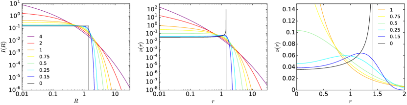
Figure 1: Left: Surface brightness profile $I(R)$ for Sérsic models with different values of $m$, focussing on models with small $m$. In this and all of the following figures, we work in dimensionless units, or equivalently, we consider a model with $R_{\text{e}}=L=M=1$. Middle: Luminosity density profile $\nu(r)$ for the same set of models. Right: Luminosity profiles of models with $m\leqslant 1$, but now shown in linear scale instead of log-log scale. All model with $m<\tfrac{1}{2}$ are characterised by a central depression.

The family of Sérsic models is defined by the surface brightness profile (2). When we replace the effective surface brightness by the total luminosity $L$ as a free parameter, we find

$$I(R)=\frac{b^{2m}}{2\pi\,m\,\Gamma(2m)}\,\frac{L}{R_{\text{e}}^{2}}\exp\left[-b\left(\frac{R}{R_{\text{e}}}\right)^{1/m}\right].$$ (3)

It is a three-parameter family with the total luminosity $L$ and the effective radius $R_{\text{e}}$ as the length and luminosity scales, and the Sérsic index $m$ a parameter that controls the shape of the surface brightness profile. The parameter $b=b(m)$ in this formula is not a free parameter in the model, but a dimensionless scaling parameter that depends on $m$, and is such that $R_{\text{e}}$ corresponds to the isophote that contains half of the emitted luminosity (we will discuss this parameter in more detail in Sect. 2.2). In the remainder of this paper, we will generally keep $L$ and $R_{\text{e}}$ fixed, and study the behaviour of the Sérsic model as a function of the Sérsic index $m$.

All Sérsic models are characterised by a finite central surface brightness. For given values of $L$ and $R_{\text{e}}$, the central surface brightness is an increasing value of the Sérsic index $m$. As we will see in the next subsection, the parameter $b(m)$ tends to zero for $m\rightarrow 0$ in a way that the central intensity converges to

$$I_{0}=\frac{L}{2\pi\,R_{\text{e}}^{2}}.$$ (4)

The fact that the total luminosity and the central surface brightness are finite even in the limit $m\rightarrow 0$ suggests that this limiting model is worth looking at in more detail. The left panel of Fig. 1 shows the intensity of the Sérsic profile for different values of $m$. For increasingly smaller values of $m$, the Sérsic intensity profile tends to approach a constant value at small radii, and then suddenly and quickly drops to zero beyond a certain radius. By using equation (50) it follows that, in the limit $m\rightarrow 0$, the Sérsic model reduces to a simple model characterised by a finite extent and a constant surface brightness,

$$I(R)=\begin{cases}\;I_{0}&R<\!\sqrt{2}\,R_{\text{e}},\\[1.00006pt] \;0&R>\!\sqrt{2}\,R_{\text{e}}.\end{cases}$$ (5)

2.2 Cumulative surface brightness and scaling parameter

For the Sérsic model, the cumulative surface brightness $S(R)$, that is the integrated flux emitted within the isophote at radius $R$,

$$S(R)=2\pi\int_{0}^{R}I(R^{\prime})\,R^{\prime}\,{\text{d}}R^{\prime},$$ (6)

can conveniently be expressed in terms of the incomplete gamma function (Paper I; Graham & Driver 2005),

$$\frac{S(R)}{L}=\frac{\gamma\left[2m,b\left(\dfrac{R}{R_{\text{e}}}\right)^{1/m}\right]}{\Gamma(2m)}.$$ (7)

In the limit $m\rightarrow 0$ this reduces to

$$\frac{S(R)}{L}=\begin{cases}\;\dfrac{R^{2}}{2R_{\text{e}}^{2}}&R<\!\sqrt{2}\,R_{\text{e}},\\[5.0pt] \;1&R>\!\sqrt{2}\,R_{\text{e}}.\end{cases}$$ (8)

As indicated in the previous section, the dimensionless scaling parameter $b$ is not a free parameter in the model, but a dimensionless number that depends on the value of $m$. Combining equation (7) with the definition of $R_{\text{e}}$ as the isophote that contains half of the emitted luminosity, it is easy to see that the value of $b$ can be found by solving the non-algebraic equation

$$\gamma(2m,b)=\frac{\Gamma(2m)}{2}.$$ (9)

Various interpolation formulae for $b$ at large $m$ have been presented in the literature (Capaccioli 1989; Paper I; Prugniel & Simien 1997). Ciotti & Bertin (1999) provide a full asymptotic expansion for $b$ for $m\rightarrow\infty$, and demonstrate that the truncated series with terms up to order $m^{-4}$ forms an excellent approximation, even for values of $m$ as small as one.

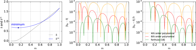
Figure 2: Left: Sérsic scaling parameter $b$ and $b^{m}$ as a function of $m$ in the range $0\leqslant m\leqslant 1$. The minimum value for $b^{m}$ is obtained at $m\approx 0.146$. Centre and right: Absolute accuracy and relative accuracy of different fitting formulae to $b$ in the range $0\leqslant m\leqslant 1$.

For the small $m\leqslant 1$ values we focus on in this paper, however, this expansion is not applicable . This was also noted by MacArthur et al. (2003), who propose a separate interpolation formula for small $m$. In Table 1 we provide accurate values for $b$ for values of $m$ between 0 and 1, obtained by solving equation (9) numerically. The variation of $b$ as a function of $m$ in this range is shown in the left panel for Fig. 2. Somewhat surprisingly, it turned out impossible to find a good polynomial interpolation formula for $b(m)$. The orange and red curves in central and right panels of Fig. 2 show the absolute and relative accuracy for the fourth and sixth order polynomial fits; no polynomial fit can reach absolute accuracy better than $10^{-3}$ over the interval $0\leqslant m\leqslant 1$, or a relative accuracy better than $10^{-3}$ over the interval $0.2\leqslant m\leqslant 1$ (relative errors are less meaningful for $m\rightarrow 0$ as $b(m)$ tends to zero in this limit).

In order to find a suitable fitting formula, one can argue that $b^{m}$ rather than $b$ is the fundamental scaling parameter in the Sérsic model. In most of the expressions for integrated quantities, the scaling parameter appears only in the combination $b^{m}$. From a mathematical point of view, the Sérsic surface brightness formula (3) can be represented in a more ‘natural’ way as

$$I(R)=\frac{1}{2\pi\,m\,\Gamma(2m)}\,\frac{L}{h^{2}}\exp\left[-\left(\frac{R}{h}\right)^{1/m}\right],$$ (10)

with the scale length $h$ instead of the effective radius as the obvious length scale (Ellis & Perry 1979; Davies et al. 1988). The parameter $b^{m}$ is then nothing but the ratio $R_{\text{e}}/h$.

The third column in Table 1 lists $b^{m}$ for Sérsic indices $m$ down to zero. Since $b$ converges to zero for $m\rightarrow 0$, the combination $b^{m}$ seems ill-defined. However, using the standard technique of asymptotic expansion, we prove in Appendix B that the leading term of the asymptotic expansion of $b(m)$ to $m\to 0$ can be written in closed form as

$$b^{m}\sim\sqrt{\,m\,\Gamma(2m)}.$$ (11)

In particular, this implies that $b^{m}$ converges to the finite value

$$\lim_{m\rightarrow 0}b^{m}=\frac{1}{\sqrt{2}}.$$ (12)

This result immediately proves the equations in Sect. 2.1 in the limit $m\rightarrow 0$.

The expression (11) only provides an accurate approximation for very small values of $m$, and it is not very useful as a practical approximation for general $m\leqslant 1$. However, it turns out that, contrary to $b$ itself, $b^{m}$ is very well fitted by a polynomial approximation over the interval $0\leqslant m\leqslant 1$. Indeed, the formula

$$b^{m}\approx\frac{1}{\sqrt{2}}+\sum_{k=1}^{4}a_{k}\,m^{k},$$ (13)

$$a_{1}=-0.45807,$$

$$a_{2}=1.83247,$$

$$a_{3}=-1.2556,$$

$$a_{4}=0.85239,$$

provides a fit with a mean absolute accuracy of $1.6\times 10^{-4}$ and a mean relative accuracy of $2.2\times 10^{-4}$ over the interval $0\leqslant m\leqslant 1$. The corresponding fitting formula for $b$,

$$b\approx\left(\frac{1}{\sqrt{2}}+\sum_{k=1}^{4}a_{k}\,m^{k}\right)^{1/m},$$ (14)

is shown as the green curve in Fig. 2. It is clearly a superior approximation to $b$ than the polynomial fits. Over the entire interval $0\leqslant m\leqslant 1$, it is characterised by a mean absolute accuracy of $1.1\times 10^{-4}$.

Curiously, the quantity $b^{m}$ does not monotonically increase as a function of $m$: the minimum value for $b^{m}$ is found for $m\approx 0.146$.

2.3 Luminosity density

Starting from a surface brightness profile $I(R)$, one can calculate the deprojected emissivity or luminosity density $\nu(r)$ through an inverse Abel transform. The general expression, valid for intensity profiles with an infinite as well as a finite extent, is (e.g., Ciotti 2000),

$$\nu(r)=-\frac{1}{\pi}\int_{r}^{r_{\text{t}}}\frac{{\text{d}}I(R)}{{\text{d}}R}\,\frac{{\text{d}}R}{\sqrt{R^{2}-r^{2}}}+{I(r_{\text{t}})\over\pi\sqrt{r_{\text{t}}^{2}-r^{2}}}$$ (15)

with $r_{\text{t}}$ the truncation radius. For models with an infinite extent, $r_{\text{t}}\to\infty$ and the formula simplifies to (Binney & Tremaine 2008)

$$\nu(r)=-\frac{1}{\pi}\int_{r}^{\infty}\frac{{\text{d}}I(R)}{{\text{d}}R}\,\frac{{\text{d}}R}{\sqrt{R^{2}-r^{2}}}.$$ (16)

It is well-known that there is no closed expression for the density corresponding the Sérsic model in terms of elementary functions or standard special functions. Baes & Van Hese (2011) used Mellin transforms to derive a general expression for the density and some related properties of the Sérsic model in terms of the Fox $H$ function. The general expression reads

$$\nu(r)=\frac{b^{3m}}{\pi^{3/2}\,\Gamma(2m)}\,\frac{L}{R_{\text{e}}^{3}}\,u^{-1}\,H^{2,0}_{1,2}\left[\left.\begin{matrix}(0,1)\\ (0,2m),(\tfrac{1}{2},1)\end{matrix}\,\right|u^{2}\right],$$ (17)

where we have introduced the reduced radial coordinate

$$u=\dfrac{b^{m}r}{R_{\text{e}}}=\frac{r}{h}.$$ (18)

This expression is maybe not directly useful for numerical calculations, because the general Fox $H$ function is not (yet) implemented in many numerical libraries or software packages. Implementations have been presented though for various programming languages, including C and MATLAB (Chergui et al. 2018), Mathematica (Shafique Ansari et al. 2012), and Python (Alhennawi et al. 2016). For rational $m$, the Fox $H$ function in expression (17) can be reduced to Meijer $G$ functions (Mazure & Capelato 2002; Baes & Gentile 2011). Contrary to the Fox $H$ function, the Meijer $G$ function is available in, for example, Maple and Mathematica, so the expression above can easily be evaluated to arbitrary precision.

A very useful application of the Fox $H$ expression (17) is that it enables to directly investigate the asymptotic behaviour of the luminosity density. Baes & Van Hese (2011) derived the asymptotic behaviour but did not discuss its implications. As already discussed in, for example, Paper I, the Sérsic models for $m>1$ have a power-law asymptotic behaviour at small radii. The leading term is

$$\nu(r)\sim\frac{b^{3m}\,\Gamma\left(\tfrac{1}{2}-\tfrac{1}{2m}\right)}{4\pi^{3/2}\,m^{2}\,\Gamma(2m)\,\Gamma\left(1-\tfrac{1}{2m}\right)}\,\frac{L}{R_{\text{e}}^{3}}\,u^{1/m-1}.$$ (19)

For large values of the Sérsic index, the model has a $r^{-1}$ central density cusp, similar to the Hernquist (1990) or NFW (Navarro et al. 1997) models, and this cusp gradually softens to a logarithmic cusp for the exponential model $m=1$. For $m<1$, the values we focus on in this paper, the Sérsic models have a finite luminosity density, given by

$$\nu_{0}=\frac{b^{3m}\,\Gamma(1-m)}{\pi^{2}\,\Gamma(1+2m)}\,\frac{L}{R_{\text{e}}^{3}}.$$ (20)

Very interesting is the leading term in the asymptotic expansion,

$$\frac{\nu(r)}{\nu_{0}}\sim\begin{cases}\;1+\dfrac{\Gamma(1-3m)}{2\,\Gamma(1-m)}\,u^{2}&0<m<\tfrac{1}{3},\\[11.99998pt] \;1+\dfrac{3\ln\tfrac{u}{2}+\gamma+\tfrac{3}{2}}{2\,\Gamma(\tfrac{3}{2})}\,u^{2}&m=\tfrac{1}{3},\\[11.99998pt] \;1+\dfrac{\sqrt{\pi}\,\Gamma\left(\tfrac{1}{2}-\tfrac{1}{2m}\right)}{2m\,\Gamma(1-m)\,\Gamma\left(1-\tfrac{1}{2m}\right)}\,u^{1/m-1}&\tfrac{1}{3}<m<\frac{1}{2},\\[13.99995pt] \;1-u^{2}&m=\tfrac{1}{2},\\[8.00003pt] \;1-\dfrac{\sqrt{\pi}\,\Gamma\left(\tfrac{3}{2}-\tfrac{1}{2m}\right)}{\Gamma(2-m)\,\Gamma\left(1-\tfrac{1}{2m}\right)}\,u^{1/m-1}&\tfrac{1}{2}<m<1.\end{cases}$$ (21)

This expansion shows that, at small radii, the luminosity density of the Sérsic model actually increases with increasing radius for all values $m<\tfrac{1}{2}$, as first noted by Trujillo et al. (2001). For $m<\tfrac{1}{3}$ this increase is parabolic, and between $m=\tfrac{1}{3}$ and $m=\tfrac{1}{2}$ the slope gradually softens towards linear. This increase is visible in the right panel of Fig. 1, where the luminosity density of the Sérsic model is shown for different values of $m$.

An explicit expression for the luminosity density corresponding to the limit $m\rightarrow 0$ can be determined by applying the deprojection recipe (16) to the surface brightness profile (5). From Equation (15) (see also Bracewell 1999), one finds

$$\nu(r)=\begin{cases}\;\dfrac{L}{2\pi^{2}R_{\text{e}}^{3}}\left(2-\dfrac{r^{2}}{R_{\text{e}}^{2}}\right)^{-1/2}&r<\!\sqrt{2}\,R_{\text{e}}.\\[5.0pt] \;0&r>\!\sqrt{2}\,R_{\text{e}}.\end{cases}$$ (22)

This formula shows that the limiting Sérsic model corresponding to $m=0$ is a spherical model with finite extent, and with a density profile that increases monotonically from a finite central value to an infinite density at the outer edge. We hence have a finite ball in which the outer layer has an infinite density, but the total luminosity is finite. The asymptotic behaviour at the centre is

$$\nu(r)\sim\nu_{0}\left(1+\tfrac{1}{2}\,u^{2}\right),$$ (23)

in agreement with the equation (21). This limiting case is interesting from a mathematical point of view, but has no direct astrophysical relevance.

2.4 Luminosity profile

The luminosity profile, that is the total luminosity emitted from a sphere with radius $r$, is given by

$$L(r)=4\pi\int_{0}^{r}\nu(r^{\prime})\,r^{\prime 2}\,{\text{d}}r^{\prime}.$$ (24)

For the Sérsic model, Baes & Van Hese (2011) showed that it can also be written in terms of the Fox $H$ function,

$$L(r)=\frac{2L}{\sqrt{\pi}\,\Gamma(2m)}\,u^{2}\,H^{2,1}_{2,3}\left[\left.\begin{matrix}(0,1),(0,1)\\ (0,2m),(\tfrac{1}{2},1),(-1,1)\end{matrix}\,\right|u^{2}\right].$$ (25)

From this general expression, the asymptotic behaviour at small $r$ can easily be derived. As all Sérsic models with $m<1$ are characterised by a finite central luminosity density, it is no surprise that $L(r)$ increases as $r^{3}$ at small radii,

$$L(r)\sim\frac{2\,\Gamma(1-m)}{3\pi\,m\,\Gamma(2m)}\,L\,u^{3}\quad 0<m<1.$$ (26)

In the limit $m\rightarrow 0$, the luminosity profile becomes

$$L(r)=\begin{cases}\;\dfrac{L}{\pi}\left[\arcsin\left(\dfrac{r}{\sqrt{2}R_{\text{e}}}\right)-\dfrac{r\sqrt{2R_{\text{e}}^{2}-r^{2}}}{R_{\text{e}}^{2}}\right]&r<\!\sqrt{2}\,R_{\text{e}},\\[5.0pt] \;L&r>\!\sqrt{2}\,R_{\text{e}}.\end{cases}$$ (27)

The asymptotic behaviour of this luminosity profile at small radii is

$$L(r)\sim\frac{\sqrt{2}\,L}{3\pi}\left(\frac{r}{R_{\text{e}}}\right)^{3}=\frac{4}{3\pi}\,L\,u^{3},$$ (28)

in agreement with the limit $m\rightarrow 0$ of expression (26).

3 Dynamical properties

Assuming a constant mass-to-light ratio, the luminosity density $\nu(r)$ can be converted to a mass density $\rho(r)$. From this mass density profile, the gravitational potential can be calculated and the dynamical structure can be investigated. This has been done in quite some detail for the Sérsic models with $m\geqslant 2$ in Paper I, and here we extend this analysis to the smaller values of the Sérsic index.

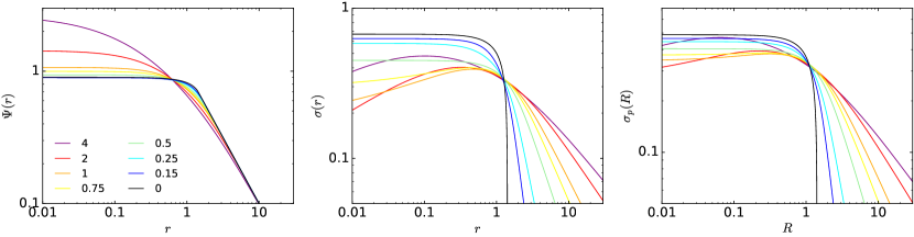
Figure 3: Left: Gravitational potential $\Psi(r)$ for the same set of Sérsic models as in Fig. 1. Middle: Velocity dispersion profile $\sigma(r)$, corresponding to an isotropic velocity distribution. Sérsic models with $m<1$ have a finite central velocity dispersion, models with $m\geqslant 1$ have a central velocity dispersion that goes to zero. Right: Observed or projected velocity dispersion profile $\sigma_{\text{p}}(R)$, again assuming an isotropic velocity distribution. All models have a finite projected velocity dispersion.

3.1 Gravitational potential

Given a spherical density profile $\rho(r)$, the (positive) gravitational potential $\Psi(r)$ can be determined as

$$\Psi(r)=4\pi G\left[\frac{1}{r}\int_{0}^{r}\rho(r^{\prime})\,r^{\prime 2}\,{\text{d}}r^{\prime}+\int_{r}^{\infty}\rho(r^{\prime})\,r^{\prime}\,{\text{d}}r^{\prime}\right].$$ (29)

For the Sérsic model, the potential can be written in terms of the Fox $H$ function (Baes & Van Hese 2011),

$$\Psi(r)=\frac{b^{m}}{\sqrt{\pi}\,\Gamma(2m)}\,\frac{GM}{R_{\text{e}}}\,u\,H^{2,1}_{2,3}\left[\left.\begin{matrix}(0,1),(0,1)\\ (0,2m),(-\tfrac{1}{2},1),(-1,1)\end{matrix}\,\right|u^{2}\right].$$ (30)

Obviously, the potential for all Sérsic models has a Keplerian decline at large radii, and a finite central value (Paper I; Baes & Van Hese 2011),

$$\Psi_{0}=\frac{2\,b^{m}\,\Gamma(1+m)}{\pi\,m\,\Gamma(2m)}\,\frac{GM}{R_{\text{e}}}.$$ (31)

At large $m$, the central potential is an increasing function of $m$. This is not the case for the entire range of Sérsic parameters, however: the minimum value of $\Psi_{0}$ is obtained for $m\approx 0.148$ (see Table 1). In the limit $m\rightarrow 0$, the gravitational potential can be calculated exactly as

$$\Psi(r)=\begin{cases}\;\dfrac{GM}{r}\left[\dfrac{2}{\pi}\arcsin\left(\dfrac{r}{\sqrt{2}R_{\text{e}}}\right)+\dfrac{r\sqrt{2R_{\text{e}}^{2}-r^{2}}}{\pi\,R_{\text{e}}^{2}}\right]&r<\!\sqrt{2}\,R_{\text{e}},\\[20.00003pt] \;\dfrac{GM}{r}&r>\!\sqrt{2}\,R_{\text{e}}.\end{cases}$$ (32)

At $r=0$, this potential reduces to

$$\Psi_{0}=\frac{2\!\sqrt{2}}{\pi}\,\frac{GM}{R_{\text{e}}},$$ (33)

in agreement with the limit $m\rightarrow 0$ of expression (31).

3.2 Velocity dispersions

Assuming an isotropic velocity distribution, the intrinsic velocity dispersion $\sigma(r)$ can be calculated using the solution of the Jeans equation,

$$\sigma^{2}(r)=\frac{1}{\nu(r)}\int_{r}^{\infty}\frac{\nu(r^{\prime})\,M(r^{\prime})\,{\text{d}}r^{\prime}}{r^{\prime 2}}.$$ (34)

An analytical expression for $\sigma(r)$ cannot be given, not even in terms of the Fox $H$ function, so we have to integrate this expression numerically. The central panel of Fig. 3 shows the velocity dispersion profile for different values of the Sérsic parameter. At large radii, the dispersion profile is relatively shallow for large $m$, and becomes gradually steeper as $m$ decreases. As already noted in Paper I, the velocity dispersion profiles for Sérsic models with $m>1$ are all characterised by a central depression, with the depression being more severe for larger values of $m$. This behaviour is expected for models in which the density behaves as a power law at small radii (e.g., see Appendix C of Bertin et al. 2002). Figure 3 also suggests that the Sérsic models with $m<1$ do not show this central depression, but have a finite central velocity dispersion, in line with the fact that Sérsic models with $m<1$ have a finite central density. In Appendix C we derive an explicit expression for $\sigma_{0}$ in terms of the Fox $H$ function,

$$\sigma_{0}^{2}=\frac{2m\,b^{m}}{\Gamma(2m)\,\Gamma(1-m)}\,\frac{GM}{R_{\text{e}}}\\ \times H^{2,3}_{4,4}\left[\left.\begin{matrix}(1,2m),(\tfrac{1}{2},1),(0,1),(0,1)\\ (0,2m),(\tfrac{1}{2},1),(-1,1),(1,1)\end{matrix}\,\right|1\right].$$ (35)

This expression is indeed finite for all $m<1$, and the numerical values are tabulated in Table 1. Clearly, $\sigma_{0}$ increases for decreasing $m$. In the limit $m\rightarrow 0$, we can explicitly calculate the entire velocity dispersion profile by substituting expressions (22) and (27) into the expression (34),

$$\sigma^{2}(r)=\begin{cases}\;\dfrac{GM}{r}\,\dfrac{2R_{\text{e}}^{2}-r^{2}}{\pi\,R_{\text{e}}^{2}}\arcsin\left(\dfrac{r}{\sqrt{2}R_{\text{e}}}\right)&r<\!\sqrt{2}\,R_{\text{e}},\\[5.0pt] \;0&r>\!\sqrt{2}\,R_{\text{e}}.\end{cases}$$ (36)

Setting $r=0$ in this expression we find a very simple expression for the central dispersion,

$$\sigma^{2}_{0}=\frac{\sqrt{2}}{\pi}\,\frac{GM}{R_{\text{e}}}.$$ (37)

This expression is in agreement with expression (35) for small values of $m$ (see Table 1).

From an observational point of view, the projected velocity dispersion or line-of-sight velocity dispersion $\sigma_{\text{p}}(R)$ is an important property. It can be obtained by projecting the velocity dispersion along the line of sight,

$$\sigma_{\text{p}}^{2}(R)=\frac{2}{I(R)}\int_{R}^{\infty}\frac{\nu(r)\,\sigma^{2}(r)\,{\text{d}}r}{\sqrt{r^{2}-R^{2}}},$$ (38)

or equivalently

$$\sigma_{\text{p}}^{2}(R)=\frac{2}{I(R)}\int_{R}^{\infty}\frac{\nu(r)\,M(r)\sqrt{r^{2}-R^{2}}\,{\text{d}}r}{r^{2}}.$$ (39)

Not surprisingly, an analytical solution cannot be obtained for general values of $m$. The right panel of Fig. 3 shows the line-of-sight velocity dispersion profiles for different values of $m$. At large radii, the line-of-sight dispersion profiles have more or less the same behaviour as the intrinsic dispersion profiles. The main difference is seen at small radii: where the intrinsic dispersion has a central depression for all $m>1$, the projected dispersion profiles converge to a finite value for all $m$. This value can be calculated explicitly (Appendix C),

$$\sigma_{\text{p},0}^{2}=\frac{4m\,b^{m}}{\pi\,\Gamma(2m)}\,\frac{GM}{R_{\text{e}}}\\ \times H^{2,3}_{4,4}\left[\left.\begin{matrix}(1-m,2m),(0,1),(0,1),(0,1)\\ (0,2m),(\tfrac{1}{2},1),(-1,1),(\tfrac{1}{2},1)\end{matrix}\,\right|1\right].$$ (40)

The central line-of-sight velocity dispersion increases with decreasing $m$, and reaches a finite value in the limit $m\rightarrow 0$,

$$\sigma_{\text{p},0}^{2}=\frac{2\!\sqrt{2}}{\pi^{2}}\,(2{\mathcal{C}}-1)\,\frac{GM}{R_{\text{e}}},$$ (41)

where ${\mathcal{C}}\simeq 0.91595...$ is Catalan’s constant. This expression can be found by combining the expressions (22), (27) and (39); a closed expression for the line-of-sight dispersion profile for arbitrary $R$ cannot be found. Table 1 shows that the expression (40) converges to the value (41) in the limit $m\rightarrow 0$.

3.3 Distribution function

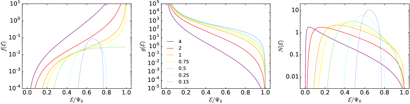
Figure 4: Left: Isotropic distribution function $f({\cal{E}})$ for the same set of Sérsic models as in Fig. 1. Only for $m\geqslant\tfrac{1}{2}$ the distribution function is positive over the entire range of binding energies, and hence physical. For models with $m<\tfrac{1}{2}$, the distribution function is negative for binding energies larger than some critical value, and hence these models cannot be supported by an isotropic velocity distributions. For these models, the (positive part of) the distribution function is shown as a dotted line. Middle: Density of states function $g({\cal{E}})$. Right: Differential energy distribution $N({\cal{E}})$.

The velocity dispersion profiles derived in the previous section are only meaningful if the isotropic distribution function is positive. It is well-known that there is a unique isotropic distribution function for each spherical potential-density pair, and that this distribution function depends only on the (positive) binding energy per unit mass ${\cal{E}}$ (e.g., Binney & Tremaine 2008). This distribution function $f({\cal{E}})$ can be calculated using Eddington’s formula,

$$f({\cal{E}})=\frac{1}{\sqrt{8}\,\pi^{2}}\int_{0}^{{\cal{E}}}\frac{{\text{d}}^{2}\rho(\Psi)}{{\text{d}}\Psi^{2}}\,\frac{{\text{d}}\Psi}{\sqrt{{\cal{E}}-\Psi}},$$ (42)

where $\rho(\Psi)$ is the mass density written as a function of the gravitational potential. The distribution function obtained in this way is not automatically guaranteed to be positive for $0<{\cal{E}}\leqslant\Psi_{0}$, which is a necessary condition for the model to be physically meaningful.

For the Sérsic models characterised by the potential-density pair (17)–(30), the Eddington formula (42) cannot be evaluated in an analytical way, so we have to use numerical means. For this purpose, expression (42) can be rewritten as

$$f({\cal{E}})=\frac{1}{\sqrt{8}\,\pi^{2}}\int_{r({\cal{E}})}^{\infty}\frac{\Delta(r)\,{\text{d}}r}{\sqrt{{\cal{E}}-\Psi(r)}},$$ (43)

where $r({\cal{E}})$ is the maximum radius reachable by a star with binding energy ${\cal{E}}$, defined implicitly by the equation $\Psi(r({\cal{E}}))={\cal{E}}$, and

$$\Delta(r)=\frac{r^{2}}{GM(r)}\left[\frac{{\text{d}}^{2}\rho(r)}{{\text{d}}r^{2}}+\frac{{\text{d}}\rho(r)}{{\text{d}}r}\left(\frac{2}{r}-\frac{4\pi\,\rho(r)\,r^{2}}{M(r)}\right)\right].$$ (44)

Binney (1982) used this approach to numerically calculate the distribution function of the de Vaucouleurs model ($m=4$), and showed that it is everywhere positive. In Paper I, this analysis was extended, and it was shown that this is the case for all Sérsic models, at least with $m>2$.

We extended this analysis even more, and calculate the distribution function for Sérsic models with arbitrary Sérsic index using expression (43), in particular focussing on the smaller values of $m$. We plot $f({\cal{E}})$ in the left panel of Fig. 4. A first important result is that $f({\cal{E}})$ is positive for all $m\geqslant\frac{1}{2}$. For all $m>\tfrac{1}{2}$ the distribution function is a strongly increasing function of the binding energy, with $f(0)=0$, and a divergence for ${\cal{E}}\rightarrow\Psi_{0}$. For the gaussian model, corresponding to $m=\tfrac{1}{2}$, the distribution function is also an increasing function, but the distribution function now converges towards a finite value at ${\cal{E}}=\Psi_{0}$.

The situation is quite different for $m<\frac{1}{2}$: for these models, the isotropic distribution function is not positive everywhere. In particular, the distribution function as obtained from equation (43) is positive at small binding energies, that is at large radii, but becomes negative for all binding energies larger than some critical value ${\cal{E}}_{\text{crit}}$. For increasingly smaller $m$, ${\cal{E}}_{\text{crit}}$ becomes increasingly smaller, or equivalently, the spatial region that corresponds to a negative distribution function becomes gradually larger. We have also plotted the distribution function, or at least the part of the distribution function that is positive, of two Sérsic models with $m<\tfrac{1}{2}$ on the left panel of Fig. 4.

The most important conclusion that should be drawn from this observation is that all Sérsic models with $m\geqslant\tfrac{1}{2}$ can be supported by an isotropic velocity dispersion tensor, since the corresponding distribution function $f({\cal{E}})$ is positive over the entire range of binding energies. Moreover, as the distribution functions of these $m\geqslant\tfrac{1}{2}$ models are monotonic, they are linearly stable with respect to both radial and non-radial perturbations, by virtue of the Doremux-Feix-Baumann theorem (Doremus et al. 1971; Binney & Tremaine 2008) and Antonov’s theorem (Antonov 1962), respectively.

The models with $m<\tfrac{1}{2}$, on the other hand, cannot be supported by an isotropic velocity dispersion tensor. This behaviour is not unexpected. In fact, our findings are a direct illustration of the results obtained by Ciotti & Pellegrini (1992), who showed that a radially decreasing density profile is a necessary condition for the positivity of the distribution function for isotropic spherical systems.

3.4 Differential energy distribution

While the distribution function does contain the full kinematical information of a dynamical system, it is important to realise that $f({\cal{E}})$ does not represent the number of stars per unit binding energy. The quantity that describes this useful characteristic is the differential energy distribution $N({\cal{E}})$. For isotropic spherically symmetric systems, $N({\cal{E}})$ can be obtained as the product of the distribution function and the so-called density of states function $g({\cal{E}})$, which represents the phase-space volume per unit binding energy (Binney & Tremaine 2008). It is calculated as

$$g({\cal{E}})=16\!\sqrt{2}\pi^{2}\int_{\cal{E}}^{\infty}\left|\,r^{2}\,\frac{{\text{d}}r}{{\text{d}}\Psi}\right|\sqrt{\Psi-{\cal{E}}}\,{\text{d}}\Psi.$$ (45)

The central panel of Fig. 4 shows the density of states function for the Sérsic models, and the right panel shows the corresponding differential energy distributions. For the de Vaucouleurs model, corresponding to $m=4$, the differential energy distribution is well approximated by a Boltzmann distribution, over a fairly large range in binding energy. This resemblance to a Boltzmann distribution was already noted by Binney (1982), and in Paper I it was argued that, of the entire family of Sérsic models, the one with $m=4$ was most Boltzmann-like. The right panel of Fig. 4 shows that, indeed, the Boltzmannian nature of the differential energy distribution decreases for decreasing $m$, and the peak of the $N({\cal{E}})$ distribution gradually moves towards larger ${\cal{E}}/\Psi_{0}$ values. As soon as $m<\tfrac{1}{2}$, the differential energy distribution becomes negative for large binding energies. In the limit $m\rightarrow 0$ the differential energy distribution, or at least the function $N({\cal{E}})$ calculated in the way described above, is characterised by an infinite peak at

$$\frac{{\cal{E}}_{\text{max}}}{\Psi_{0}}=\frac{\Psi(\sqrt{2}R_{\text{e}})}{\Psi_{0}}=\frac{\pi}{4},$$ (46)

and negative values for all ${\cal{E}}>{\cal{E}}_{\text{max}}$.

We note that this does not necessarily imply that the Sérsic models with $m<\tfrac{1}{2}$ are unphysical: it still possible to self-consistently generate these density distributions with anisotropic distribution functions that favour tangential over radial orbits. In principle, one can always build dynamical models that only contain purely circular orbits for arbitrary density profiles (leaving aside stability issues). Whether self-consistent and stable dynamical models with a gradual preference for tangential orbits can be constructed for Sérsic models with $m<\tfrac{1}{2}$ is currently unclear. Such models have been constructed for different spherical potential-density pairs (e.g., Dejonghe 1987; Baes & Dejonghe 2002; Baes & Van Hese 2007; Nguyen & Lingam 2013; Lingam & Nguyen 2014).

4 Summary

The goal of this paper was to investigate in detail the main photometric, intrinsic, and dynamic properties of the Sérsic model, with a particular focus on the subset of models with Sérsic index $m<1$. This small $m$ regime was not discussed in most previous studies on the Sérsic model (e.g., Paper I; Paper II; Mazure & Capelato 2002; Graham & Driver 2005). Sérsic models with small values of $m$ are very relevant, though, in particular for low-luminosity and dwarf elliptical galaxies. Indeed, the Sérsic index correlates with luminosity (Caon et al. 1993; Graham & Guzmán 2003), and values down to $m\approx 0.4$ have been found (e.g., Young & Currie 1994; Binggeli & Jerjen 1998; MacArthur et al. 2003).

We show that there is no polynomial fitting formula for the Sérsic scaling parameter $b$ with an absolute accuracy better than $10^{-3}$ over the interval $0\leqslant m\leqslant 1$. Instead we present a different fitting formula, based on a polynomial approximation for $b^{m}$, that has a mean absolute accuracy of $1.1\times 10^{-4}$ over this interval. We also derive the formal asymptotic expansion of $b(m)$ for $m\to 0$ that can be used to compute all the analytical limiting formulae presented in this paper.

While the surface brightness profile of all Sérsic models is finite at the centre, the corresponding luminosity density shows a rich variety, depending on the value of $m$. For $m>1$, the luminosity density is characterised by a $r^{1/m-1}$ cusp, while for $m<1$ the central luminosity density is finite. For $m<\tfrac{1}{2}$, the luminosity density profile increases with increasing radius at small radii, resulting in a central luminosity density depression. All Sérsic models have a finite potential well, and a finite central projected velocity dispersion (when assuming an anisotropic velocity distribution). The intrinsic velocity dispersion drops to zero for models with $m\geqslant 1$, but assumes a finite value for $m<1$. All of these properties can be calculated analytically.

All Sérsic models with $m\geqslant\tfrac{1}{2}$ can be supported by an isotropic velocity dispersion tensor, and these isotropic models are stable to both radial and non-radial perturbations. For decreasing value of $m$, the differential energy distribution deviates more and more from a Boltzmannian distribution. These results directly extend the conclusions of Paper I. However, we find that Sérsic models with $m<\tfrac{1}{2}$ cannot be supported by an isotropic velocity distribution, which is a logical consequence of their particular density profile.

The Sérsic model corresponding to the limit $m\rightarrow 0$ is characterised by a finite extent and a uniform surface brightness distribution. In 3D, this translates to a ball in which the density increases from the centre to an outer, infinite-density skin. Most of the intrinsic and dynamical properties can be expressed in terms of elementary functions for this extreme model.

Finally, we note that we have made use of the analytical expressions based on the Fox $H$ function, derived by Baes & Van Hese (2011). Our analysis again demonstrates the power of the underestimated Fox $H$ function as a tool for analytical work.

Appendix A Numerical values

In Table 1 we present numerical values for a number of important properties of the Sérsic models, as a function of $m$. All quantities are given in dimensionless units, or equivalently, for a model with $R_{\text{e}}=L=M=1$.

Table 1: Numerical values for a number of important properties of the Sérsic models, as a function of the Sérsic index $m$. The different columns correspond to the scaling parameter $b$, the ratio $b^{m}=R_{\text{e}}/h$, the central surface brightness $I_{0}$, the central luminosity density $\nu_{0}$, the central value of the gravitational potential $\Psi_{0}$, the central velocity dispersion $\sigma_{0}$, and the central projected velocity dispersion $\sigma_{\text{p},0}$. All quantities are given in dimensionless units, or equivalently, for a model with $R_{\text{e}}=L=M=1$.

$m$	$b$	$b^{m}$	$I_{0}$	$\nu_{0}$	$\Psi_{0}$	$\sigma_{0}$	$\sigma_{\text{p},0}$
$0.0$	$0.0$	$0.7071067812$	$0.1591549431$	$0.03582244802$	$0.9003163162$	$0.6709382670$	$0.4882770668$
$0.1$	$0.02074633919$	$0.6787254708$	$0.1597040458$	$0.03687117924$	$0.8954110224$	$0.6467405417$	$0.4745932365$
$0.2$	$0.1450781416$	$0.6797048938$	$0.1657441274$	$0.04174912260$	$0.8955714657$	$0.6052798406$	$0.4549379359$
$0.3$	$0.3157020170$	$0.7075924771$	$0.1783670066$	$0.05214840909$	$0.9049229140$	$0.5576761459$	$0.4365182562$
$0.4$	$0.5013512264$	$0.7586768505$	$0.1967139352$	$0.07074452800$	$0.9202187043$	$0.5054510861$	$0.4198025544$
$0.5$	$0.6931471806$	$0.8325546112$	$0.2206356002$	$0.1036366539$	$0.9394372787$	$0.4490044158$	$0.4046143026$
$0.6$	$0.8879362135$	$0.9311701833$	$0.2504981367$	$0.1646935035$	$0.9614737847$	$0.3883701725$	$0.3907268693$
$0.7$	$1.084371511$	$1.058338681$	$0.2870242952$	$0.2892627286$	$0.9857010672$	$0.3231072572$	$0.3779411016$
$0.8$	$1.281796137$	$1.219706019$	$0.3312367088$	$0.5903862892$	$1.011747061$	$0.2516350723$	$0.3660931503$
$0.9$	$1.479856427$	$1.422976161$	$0.3844538418$	$1.656657118$	$1.039383734$	$0.1684024227$	$0.3550500768$
$1.0$	$1.678346990$	$1.678346990$	$0.4483153816$	$\infty$	$1.068468879$	$0.0$	$0.3447039338$
$1.5$	$2.674060314$	$4.372771642$	$1.014407550$	$\infty$	$1.233536106$	$0.0$	$0.3008238298$
$2.0$	$3.672060749$	$13.48403014$	$2.411450297$	$\infty$	$1.430700033$	$0.0$	$0.2658868180$
$2.5$	$4.670908883$	$47.15236589$	$5.897607399$	$\infty$	$1.662679605$	$0.0$	$0.2367684306$
$3.0$	$5.670161189$	$182.2998096$	$14.69230924$	$\infty$	$1.934261054$	$0.0$	$0.2118423541$
$3.5$	$6.669637075$	$766.2274547$	$37.07959732$	$\infty$	$2.251549732$	$0.0$	$0.1901483907$
$4.0$	$7.669249443$	$3459.485015$	$94.48274697$	$\infty$	$2.621876860$	$0.0$	$0.1710622608$
$4.5$	$8.668951184$	$16628.36345$	$242.5415290$	$\infty$	$3.053889794$	$0.0$	$0.1541466369$
$5.0$	$9.668714615$	$84497.47049$	$626.2886060$	$\infty$	$3.557722251$	$0.0$	$0.1390769232$

Appendix B Asymptotic expansion of the scaling parameter for $m\rightarrow 0$

The scaling parameter $b$ is defined through equation (9). In order to find an asymptotic form for $b(m)$ for $m\rightarrow 0$, we take the Laurent expansion of the right-hand expression,

$$\frac{\Gamma(2m)}{2}=\frac{1}{4m}-\frac{\gamma}{2}+\frac{1}{2}\left(\frac{\pi^{2}}{6}+\gamma^{2}\right)m+{\mathcal{O}}(m^{2})$$ (47)

with $\gamma\simeq 0.577216...$ the Euler-Mascheroni constant. The left-hand side of (9) can be written as

$$\gamma(2m,b)=\int_{0}^{b}t^{2m-1}\,e^{-t}\,{\text{d}}t=\frac{b^{2m}}{2m}+\sum_{j=1}^{\infty}\frac{(-1)^{j}\,b^{2m+j}}{(2m+j)\,j!}$$ (48)

We search for a solution for $b^{2m}$ of the form

$$b^{2m}=X_{0}+X_{1}\,m+X_{2}\,m^{2}+\cdots$$ (49)

Inserting this expansion into expression (48) and equating the result to (47), we can determine each of the coefficients by using order balance. After some calculation, one finds

$$b^{2m}=\frac{1}{2}-\gamma\,m+\left(\frac{\pi^{2}}{6}+\gamma^{2}\right)m^{2}+\cdots$$ (50)

Repeating the treatment at all orders, it follows that the leading term of the asymptotic expansion of $b(m)$ for $m\to 0$ can be obtained in closed form as

$$b^{m}\sim\sqrt{\,m\,\Gamma(2m)}.$$ (51)

This is also shown in Fig. 5, where we compare the numerically determined values of $b^{m}$ and the approximation (51).

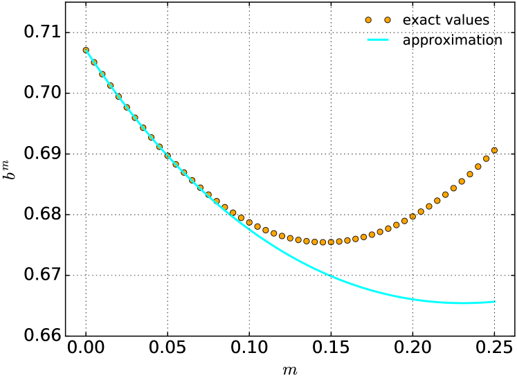
Figure 5: The quantity $b^{m}$ for very small values of $m$. The yellow dots correspond to the exact value determined by numerical evaluation of equation (9), the cyan line is the approximation (51).

Appendix C Exact expressions for the central dispersions

Assuming an isotropic velocity dispersion tensor, the intrinsic velocity dispersion profile $\sigma(r)$ can be derived using the solution of the Jeans equation,

$$\sigma^{2}(r)=\frac{G}{\nu(r)}\int_{r}^{\infty}\frac{M(r^{\prime})\,\nu(r^{\prime})\,{\text{d}}r^{\prime}}{r^{\prime 2}}.$$ (52)

In the case $m<1$, the central luminosity is finite, and we obtain for $r=0$,

$$\sigma_{0}^{2}=\frac{G}{\nu_{0}}\int_{0}^{\infty}\frac{M(r)\,\nu(r)\,{\text{d}}r}{r^{2}}.$$ (53)

Substituting the expressions (17) and (25) for $\nu(r)$ and $M(r)$, this becomes

$$\sigma_{0}^{2}=\frac{2m\,b^{m}}{\Gamma(2m)\,\Gamma(1-m)}\,\frac{GM}{R_{\text{e}}}\\ \qquad\quad\times\int_{0}^{\infty}H^{2,1}_{2,3}\left[\left.\begin{matrix}(0,1),(0,1)\\ (0,2m),(\tfrac{1}{2},1),(-1,1)\end{matrix}\,\right|x\right]\\ \times H^{2,0}_{1,2}\left[\left.\begin{matrix}(0,1)\\ (0,2m),(\tfrac{1}{2},1)\end{matrix}\,\right|x\right]x^{-1}\,dx.$$ (54)

The integral in this expression is a particular case of a Mellin transform of the product of two Fox $H$ functions, which can be evaluated again as a Fox $H$ function (Mathai et al. 2009, §2.3),

$$\sigma_{0}^{2}=\frac{2m\,b^{m}}{\Gamma(2m)\,\Gamma(1-m)}\,\frac{GM}{R_{\text{e}}}\,\\ \times H^{2,3}_{4,4}\left[\left.\begin{matrix}(1,2m),(\tfrac{1}{2},1),(0,1),(0,1)\\ (0,2m),(\tfrac{1}{2},1),(-1,1),(1,1)\end{matrix}\,\right|1\right].$$ (55)

In the special case $m=\tfrac{1}{2}$, corresponding to a Gaussian model, this Fox $H$ function reduces to a Meijer $G$ function, which can be expressed in terms of elementary functions,

$$\sigma_{0}^{2}=\sqrt{\frac{b}{\pi}}\,\frac{GM}{R_{\text{e}}}\,G^{1,2}_{2,2}\left[\left.\begin{matrix}\tfrac{1}{2},0\\ \tfrac{1}{2},-1\end{matrix}\,\right|1\right]=\frac{(4-\pi)\sqrt{b}}{2\sqrt{\pi}}\,\frac{GM}{R_{\text{e}}}.$$ (56)

The projected velocity dispersion profile can be found through the formula

$$\sigma_{\text{p}}^{2}(R)=\frac{2}{I(R)}\int_{R}^{\infty}\frac{M(r)\,\nu(r)\sqrt{r^{2}-R^{2}}\,{\text{d}}r}{r^{2}}.$$ (57)

For $R=0$, this expression reduces to

$$\sigma_{\text{p},0}^{2}=\frac{2}{I_{0}}\int_{0}^{\infty}\frac{M(r)\,\nu(r)\,{\text{d}}r}{r}.$$ (58)

This expression is very similar to expression (53), and can be evaluated in a similar way. The resulting expression is

$$\sigma_{\text{p},0}^{2}=\frac{4m\,b^{m}}{\pi\,\Gamma(2m)}\,\frac{GM}{R_{\text{e}}}\\ \times H^{2,3}_{4,4}\left[\left.\begin{matrix}(1-m,2m),(0,1),(0,1),(0,1)\\ (0,2m),(\tfrac{1}{2},1),(-1,1),(\tfrac{1}{2},1)\end{matrix}\,\right|1\right].$$ (59)

For the Gaussian model $m=\tfrac{1}{2}$, this expression can be simplified to a Meijer $G$ function and expressed in terms of elementary functions,

$$\sigma_{\text{p},0}^{2}=\frac{2\!\sqrt{b}}{\pi}\,\frac{GM}{R_{\text{e}}}\,G^{1,2}_{2,2}\left[\left.\begin{matrix}0,0\\ \tfrac{1}{2},-1\end{matrix}\,\right|1\right]\\ =\frac{[2\ln(1+\sqrt{2})-\sqrt{2}]\!\sqrt{b}}{\sqrt{\pi}}\,\frac{GM}{R_{\text{e}}}.$$ (60)

Also for other integer and half-integer values of $m$, the Fox $H$ function in expression (59) can be reformed to a Meijer $G$ function, now by application of Gauss’ multiplication theorem. One finds after some calculation

$$\sigma_{\text{p},0}^{2}=\frac{4(2m)^{m}b^{m}}{(2\pi)^{2m}\,\Gamma(2m)}\,\frac{GM}{R_{\text{e}}}\\ \times G^{2m,2m+1}_{2m+1,2m+1}\left[\left.\begin{matrix}-\tfrac{m-1}{2m},-\tfrac{m-1}{2m},\ldots,\tfrac{m-1}{2m},0,0\\[3.00003pt] \tfrac{1}{2m},\tfrac{2}{2m},\ldots,\tfrac{2m-1}{2m},\tfrac{1}{2},-1\end{matrix}\,\right|1\right].$$ (61)

Setting $m=1$ in this expression, we find a surprisingly simple result for the central projected velocity dispersion of the exponential model,

$$\sigma_{\text{p},0}^{2}=\frac{2b}{\pi^{2}}\,\frac{GM}{R_{\text{e}}}\,G^{2,3}_{3,3}\left[\left.\begin{matrix}0,0,0\\ \tfrac{1}{2},\tfrac{1}{2},-1\end{matrix}\,\right|1\right]=\frac{(\pi-3)\,b}{2}\,\frac{GM}{R_{\text{e}}}.$$ (62)

References

- Alhennawi et al. (2016) Alhennawi, H. R., El Ayadi, M. M. H., Alouini, M.-S., Ismail, M. H., & Mourad, H.-A. M. 2016, IEEE Transactions on Vehicular Technology, 65, 1957
- Allen et al. (2006) Allen, P. D., Driver, S. P., Graham, A. W., et al. 2006, MNRAS, 371, 2
- Antonov (1962) Antonov, V. A. 1962, Solution of the problem of stability of stellar system (Vestnik Leningradskogo Universiteta, Leningrad)
- Baes & Dejonghe (2002) Baes, M. & Dejonghe, H. 2002, A&A, 393, 485
- Baes & Gentile (2011) Baes, M. & Gentile, G. 2011, A&A, 525, A136
- Baes & Van Hese (2007) Baes, M. & Van Hese, E. 2007, A&A, 471, 419
- Baes & Van Hese (2011) Baes, M. & Van Hese, E. 2011, A&A, 534, A69
- Bertin et al. (2002) Bertin, G., Ciotti, L., & Del Principe, M. 2002, A&A, 386, 149
- Binggeli & Jerjen (1998) Binggeli, B. & Jerjen, H. 1998, A&A, 333, 17
- Binney (1982) Binney, J. 1982, MNRAS, 200, 951
- Binney & Tremaine (2008) Binney, J. & Tremaine, S. 2008, Galactic Dynamics: Second Edition (Princeton University Press)
- Bracewell (1999) Bracewell, R. 1999, The Fourier Transform and Its Applications, 3rd ed. (New York: McGraw-Hill)
- Bruce et al. (2012) Bruce, V. A., Dunlop, J. S., Cirasuolo, M., et al. 2012, MNRAS, 427, 1666
- Caon et al. (1993) Caon, N., Capaccioli, M., & D’Onofrio, M. 1993, MNRAS, 265, 1013
- Capaccioli (1989) Capaccioli, M. 1989, in World of Galaxies (Le Monde des Galaxies), ed. H. G. Corwin, Jr. & L. Bottinelli, 208–227
- Cardone (2004) Cardone, V. F. 2004, A&A, 415, 839
- Cardone et al. (2005) Cardone, V. F., Piedipalumbo, E., & Tortora, C. 2005, MNRAS, 358, 1325
- Chergui et al. (2018) Chergui, H., Benjillali, M., & Alouini, M.-S. 2018, ArXiv e-prints
- Ciotti (1991) Ciotti, L. 1991, A&A, 249, 99
- Ciotti (2000) Ciotti, L. 2000, Lecture notes on stellar dynamics (Scuola Normale Superiore, Pisa)
- Ciotti & Bertin (1999) Ciotti, L. & Bertin, G. 1999, A&A, 352, 447
- Ciotti & Lanzoni (1997) Ciotti, L. & Lanzoni, B. 1997, A&A, 321, 724
- Ciotti & Pellegrini (1992) Ciotti, L. & Pellegrini, S. 1992, MNRAS, 255, 561
- Davies et al. (1988) Davies, J. I., Phillipps, S., Cawson, M. G. M., Disney, M. J., & Kibblewhite, E. J. 1988, MNRAS, 232, 239
- de Vaucouleurs (1948) de Vaucouleurs, G. 1948, Annales d’Astrophysique, 11, 247
- de Vaucouleurs & Capaccioli (1979) de Vaucouleurs, G. & Capaccioli, M. 1979, ApJS, 40, 699
- Dehnen (1993) Dehnen, W. 1993, MNRAS, 265, 250
- Dejonghe (1987) Dejonghe, H. 1987, MNRAS, 224, 13
- D’Onofrio et al. (1994) D’Onofrio, M., Capaccioli, M., & Caon, N. 1994, MNRAS, 271, 523
- Doremus et al. (1971) Doremus, J.-P., Feix, M. R., & Baumann, G. 1971, Physical Review Letters, 26, 725
- Einasto (1965) Einasto, J. 1965, Trudy Astrofizicheskogo Instituta Alma-Ata, 5, 87
- Elíasdóttir & Möller (2007) Elíasdóttir, Á. & Möller, O. 2007, J. Cosmology Astropart. Phys., 7, 006
- Ellis & Perry (1979) Ellis, G. F. R. & Perry, J. J. 1979, MNRAS, 187, 357
- Gadotti (2009) Gadotti, D. A. 2009, MNRAS, 393, 1531
- Graham & Driver (2005) Graham, A. W. & Driver, S. P. 2005, PASA, 22, 118
- Graham & Guzmán (2003) Graham, A. W. & Guzmán, R. 2003, AJ, 125, 2936
- Gutiérrez et al. (2004) Gutiérrez, C. M., Trujillo, I., Aguerri, J. A. L., Graham, A. W., & Caon, N. 2004, ApJ, 602, 664
- Haubold et al. (2007) Haubold, H. J., Mathai, A. M., & Saxena, R. K. 2007, Bulletin of the Astronomical Society of India, 35, 681
- Henon (1959) Henon, M. 1959, Annales d’Astrophysique, 22, 126
- Hernquist (1990) Hernquist, L. 1990, ApJ, 356, 359
- Jaffe (1983) Jaffe, W. 1983, MNRAS, 202, 995
- Lange et al. (2016) Lange, R., Moffett, A. J., Driver, S. P., et al. 2016, MNRAS, 462, 1470
- Lingam & Nguyen (2014) Lingam, M. & Nguyen, P. H. 2014, MNRAS, 440, 2636
- MacArthur et al. (2003) MacArthur, L. A., Courteau, S., & Holtzman, J. A. 2003, ApJ, 582, 689
- Mathai et al. (2009) Mathai, A. M., Saxena, R. K., & Haubold, H. J. 2009, The H-Function: Theory and Applications (Springer-Verlag New York)
- Mazure & Capelato (2002) Mazure, A. & Capelato, H. V. 2002, A&A, 383, 384
- Möllenhoff & Heidt (2001) Möllenhoff, C. & Heidt, J. 2001, A&A, 368, 16
- Navarro et al. (1997) Navarro, J. F., Frenk, C. S., & White, S. D. M. 1997, ApJ, 490, 493
- Nguyen & Lingam (2013) Nguyen, P. H. & Lingam, M. 2013, MNRAS, 436, 2014
- Plummer (1911) Plummer, H. C. 1911, MNRAS, 71, 460
- Poveda et al. (1960) Poveda, A., Iturriaga, R., & Orozco, I. 1960, Boletin de los Observatorios Tonantzintla y Tacubaya, 2, 3
- Prugniel & Simien (1997) Prugniel, P. & Simien, F. 1997, A&A, 321, 111
- Retana-Montenegro et al. (2012a) Retana-Montenegro, E., Frutos-Alfaro, F., & Baes, M. 2012a, A&A, 546, A32
- Retana-Montenegro et al. (2012b) Retana-Montenegro, E., Van Hese, E., Gentile, G., Baes, M., & Frutos-Alfaro, F. 2012b, A&A, 540, A70
- Salo et al. (2015) Salo, H., Laurikainen, E., Laine, J., et al. 2015, ApJS, 219, 4
- Saxena et al. (2006) Saxena, R. K., Mathai, A. M., & Haubold, H. J. 2006, Ap&SS, 305, 289
- Sérsic (1968) Sérsic, J. L. 1968, Atlas de Galaxias Australes (Observatorio Astronomico, Cordoba, Argentina)
- Shafique Ansari et al. (2012) Shafique Ansari, I., Yilmaz, F., Alouini, M.-S., & Kucur, O. 2012, ArXiv e-prints
- Tremaine et al. (1994) Tremaine, S., Richstone, D. O., Byun, Y.-I., et al. 1994, AJ, 107, 634
- Trujillo et al. (2001) Trujillo, I., Aguerri, J. A. L., Cepa, J., & Gutiérrez, C. M. 2001, MNRAS, 321, 269
- Trujillo et al. (2002) Trujillo, I., Asensio Ramos, A., Rubiño-Martín, J. A., et al. 2002, MNRAS, 333, 510
- van der Wel et al. (2012) van der Wel, A., Bell, E. F., Häussler, B., et al. 2012, ApJS, 203, 24
- Van Hese et al. (2009) Van Hese, E., Baes, M., & Dejonghe, H. 2009, ApJ, 690, 1280
- Young & Currie (1994) Young, C. K. & Currie, M. J. 1994, MNRAS, 268, L11
- Young (1976) Young, P. J. 1976, AJ, 81, 807
- Zaninetti (2012) Zaninetti, L. 2012, Rev. Mexicana Astron. Astrofis., 48, 209