On the Global Minimizers of Real Robust Phase Retrieval with Sparse Noise

Abstract

We study a class of real robust phase retrieval problems under a Gaussian assumption on the coding matrix when the received signal is sparsely corrupted by noise. The goal is to establish conditions on the sparsity under which the input vector can be exactly recovered. The recovery problem is formulated as the minimization of the $\ell_{1}$ norm of the residual. The main contribution is a robust phase retrieval counterpart to the seminal paper by Candes and Tao on compressed sensing ($\ell_{1}$ regression) [Decoding by linear programming. IEEE Transactions on Information Theory, 51(12):4203–4215, 2005]. Our analysis depends on a key new property on the coding matrix which we call the Absolute Range Property (ARP). This property is an analogue to the Null Space Property (NSP) in compressed sensing. When the residuals are computed using squared magnitudes, we show that ARP follows from a standard Restricted Isometry Property (RIP). However, when the residuals are computed using absolute magnitudes, a new and very different kind of RIP or growth property is required. We conclude by showing that the robust phase retrieval objectives are sharp with respect to their minimizers with high probability.

1 Introduction

Phase retrieval has been widely studied in machine learning, signal processing and optimization. The goal of phase retrieval is to recover a signal $x$ provided the observations of the amplitude of its linear measurements:

$$|\left\langle a_{i},\,x\right\rangle|=b_{i},\quad 1\leq i\leq m$$ (1.1)

where $a_{i}\in\mathbb{C}^{n}$ or $\mathbb{R}^{n}$, $b_{i}\in\mathbb{R}$ are observations, and $x$ is an unknown variable we wish to recover (e.g. see [27]). A well studied form of the phase retrieval problem is

$$|\left\langle a_{i},\,x\right\rangle|^{2}=b_{i},\quad 1\leq i\leq m,$$ (1.2)

where $b_{i}$ now represent the squared magnitudes of the observations. It is shown in [28] that the phase retrieval problem is NP-hard. Recent work on the phase retrieval problem [15, 24, 20, 11, 10] focuses on the real phase retrieval problem where it is assumed that $a_{i}\in\mathbb{R}^{n}$ for each $i=1,2,...,m$. This is the line of inquiry we follow. In the following discussion the $m$ rows of the matrix $A\in\mathbb{R}^{m\times n}$ are the vectors $a_{i}\in\mathbb{R}^{n}$.

The two most popular approaches to the real phase retrieval problem are through semidefinite programming relaxations [2, 10, 12, 17, 21, 26, 31] and convex-composite optimization [5, 20, 24]. These approaches formulate real phase retrieval problem as an optimization problem of the form

$$\min_{x}\rho(|Ax|^{2}-b),$$ (1.3)

where $\rho$ is chosen to be either the $\ell_{1}$ or the square of $\ell_{2}$ norm, and, for any vector $z\in\mathbb{R}^{m}$, $|z|$ and $z^{2}$ are vectors in $\mathbb{R}^{m}$ whose components are the absolute value and squares of those in $z$. The objective in (1.3) is a composition of a convex and a smooth function, and is called convex-composite. This structure plays a key role in both optimality conditions and algorithm development for (1.3) [5].

In the noiseless case, when there exists a vector $x_{*}\in\mathbb{R}^{n}$ such that $|Ax_{*}|^{2}=b$ (or, $|Ax_{*}|=b$), a gradient based method called Wirtinger Flow (WF) was introduced by [11] to solve the smooth problem

$$\min_{x}\left\||Ax|^{2}-b\right\|_{2}^{2}.$$

WF admits a linear convergence rate when properly initialized. Further work along this line includes the Truncated Wirtinger Flow (TWF), e.g., see [17]. Truncated Wirtinger Flow requires $m\geq Cn$ measurements as opposed to the $m\geq Cn\log n$ measurements in WF to obtain a linear rate. A similar approach using sub-gradient is used to minimize $\min_{x}\left\||Ax|-b\right\|_{2}^{2}$ in [32] for the noiseless case.

Contributions. In this paper we address two forms of the robust phase retrieval problem, where the optimization objective takes the form

$$\min_{x}f_{p}(x):=\left\||Ax|^{p}-b\right\|_{1}\quad\mbox{for $p=1,2$},$$ (1.4)

and it is assumed that the matrix $A$ satisfies the following Gaussian assumption:

$$\mathrm{G:}\qquad\mbox{The entries of $A$ are i.i.d. standard Gaussians $N(0,1)$.}$$

Our goal is to establish a robust phase retrieval counterpart to the seminal paper by Candes and Tao on compressed sensing ($\ell_{1}$ regression) [13].

Compressed sensing problems [22] take the form

$$\min_{y}\left\|y\right\|_{1}\text{ such that }\Phi y=c,$$ (1.5)

where $\Phi\in\mathbb{R}^{n\times N},y\in\mathbb{R}^{N},c\in\mathbb{R}^{n}$. This problem is known to be equivalent to the $\ell_{1}$ linear regression problem

$$\min_{x}\left\|Ax-b\right\|_{1},$$ (1.6)

where $\Phi b=-c$ and $A\in\mathbb{R}^{N\times(N-n)}$ (e.g., the columns of $A$ form basis of $\text{Null}(\Phi)$). In [13] it is shown that there is a universal constant $s\in(0,1)$ such that, under suitable conditions on $A$ (e.g., Assumption G), if $x^{*}$ satisfies $\left\|Ax_{*}-b\right\|_{0}\leq sm$, then $x^{*}$ is the unique solution to (1.6), with high probability. We prove similar exact recovery results for the two robust phase retrieval problems (1.4). In particular, we show that $\{x_{*},-x_{*}\}=\mathop{\mathrm{argmin}}f_{p}$ with high probability, when $m\geq 2n-1$ (Theorem 5). In this situation, the solution set to $\min f_{p}$ and the $\ell_{0}$ phase retrieval problem coincide, that is,

$$\{x_{*},-x_{*}\}=\mathop{\mathrm{argmin}}_{x}\left\||Ax|^{p}-b\right\|_{0}.$$ (1.7)

Thus, the $\ell_{0}$ phase retrieval problem can be solved by the $\ell_{1}$ phase retrieval problem $\min f_{p}$, when there exists an $x_{*}$ with sufficiently sparse noise.

A key underlying structural requirement used by [13] is the Restricted Isometry Property (RIP). We also make use of an RIP property in the $p=2$ case. However, in the $p=1$ case a new property, which we call the p-Absolute Growth Property (p-AGP) (see Definition 3), is required. When $p=2$, RIP implies 2-AGP. The p-AGP holds under Assumption G, with high probability (see Lemmas 6 and 12). A second key property, which mimics the so-called Null Space Property (NSP) in compressed sensing [18, 19, 23, 25], is also introduced. We call this the p-Absolute Range Property (p-ARP) (see Definition 1), and show that p-AGP implies p-ARP under Assumption G with high probablility. In [9], it is shown that, for problem (1.5), if $\Phi$ satisfies RIP with parameter $\delta_{2s}<\sqrt{2}-1$, then $\Phi$ satisfies NSP of order $s$. Correspondingly, we show that the p-AGP implies the p-ARP with high probability under Assumption G. (see Lemmas 7 and 13).

There are separate classes of methods for solving (1.4) for $p=2$ and $p=1$. When $p=1$, one can apply a smoothing method to the absolute value function [1, 27], or use other relaxation techniques that preserve the nonsmooth objective but introduce auxiliary variables [34]. When $p=2$, the solution methods typically exploit the convex-composite structure of the objective $f_{2}$. These methods rely on two key conditions on the function $f_{2}$: weak convexity (i.e., $f+\frac{\rho}{2}\left\|\cdot\right\|^{2}$ is convex for some $\rho>0$) and sharpness (i.e., $f(x)-\min f\geq c\cdot\text{dist}(x,\mathcal{X})$ for some $c>0$ where $\mathcal{X}$ is the set of minimizers of $f$). Under these two properties, Duchi and Ruan [24], Drusvyatskiy, Davis and Paquette [20] and Charisopoulos, et al.[15] establish convergence and iteration complexity results for prox-linear and subgradient algorithms. Recently [33] and [16] considered gradient-based methods for the problem $\min_{x}f_{2}(x)$ when the noise is $sm$ sparse for some $s<1$. To establish locally linear convergence of their algorithms the authors of [33] require that the measurements satisfy $m\geq cn\log n$ for $c>0$, while the authors of [16] require that $s<c/\log m$ for some $c>0$. The results in [24] and [15] require $m\geq cn$ for some $c>0$ and for some $s\in[0,\frac{1}{2})$ sufficiently small.

Conditions for the weak convexity of $f_{2}$ follow from results in [24, 20] under assumptions weaker than Assumption G. In the noiseless case, the sharpness of $f_{2}$ also follows from results in [24, 20]. In the noisy case, sharpness is established in [24, 20] under same assumptions on the sparsity of the noise.

We establish sharpness for both $f_{1}$ and $f_{2}$ under Assumption G uniformly for all possible supports of the sparse noise. Our result for $p=2$ case has a similar flavor to those in [24, 15], but more closely parallels the result of Candes and Tao in the compressed sensing case. When $p=1$, our result has no precedence in the literature and requires a new approach. The function $f_{1}$ is not weakly convex since it is not even subdifferentially regular [27].

This paper is organized as follows. In section 2, we introduce the new properties p-ARP and p-AGP and provide a detailed description of how our program of proof parallels the program used in compressed sensing. In Section 3, we show that if $A$ satisfies p-ARP and the residual $|\,|Ax_{*}|^{p}-b|$ is sufficiently sparse, then $\{\pm x_{*}\}\subset\mathop{\mathrm{argmin}}f_{p}$ with equality under Assumption G. In section 4, we show that Assumption G implies that p-AGP implies p-ARP with high probability. In the last section we show that $f_{p}$ is sharp with respect to $\mathop{\mathrm{argmin}}f_{p}$, with high probability.

1.1 Notation

Lower case letters (i.e. $x$, $y$) denote vectors, while $x_{i}$ denotes the $i$th component of the $x$. $c_{0},c_{1},c_{2},\tilde{c_{0}},\tilde{c_{1}},C$ denote universal constants. $\left\|x\right\|$, $\left\|x\right\|_{1}$ denote the Euclidean and $\ell_{1}$ norms of vector x, while $\left\|x\right\|_{0}$ denotes the $\ell_{0}$ ‘norm’ $|\{i|x_{i}\neq 0\}|$. For a matrix $X$, $\left\|X\right\|_{F}$ denotes the Frobenius and $\left\|X\right\|$ denotes the $\ell_{2}$ operator norm. When $x=(x_{i})_{1\leq i\leq n}$ is a vector, $|x|:=(|x_{i}|)_{1\leq i\leq n}$ and $x^{p}:=(x_{i}^{p})_{1\leq i\leq m}$. For a vector $v\in\mathbb{R}^{m}$, and $T\in[m]:=\{1,2,...,m\}$, $v_{T}$ is defined to be a vector in $\mathbb{R}^{m}$ where the $i$th entry is $v_{i}$ if $i\in T$ and $0$ else where. $\mathrm{supp}(x):=\{i|x_{i}\neq 0\}$. We say a vector $x$ is $L$ sparse if $\left\|x\right\|_{0}:=|\mathrm{supp}(x)|\leq L$.

2 The Roadmap

Recall from the compressed sensing literature [18, 19] that a matrix $\Phi\in\mathbb{R}^{m\times n}$ satisfies Null Space Property (NSP) of order $L$ at $\psi\in(0,1)$ if

$$\left\|y_{T}\right\|_{1}\leq\psi\left\|y_{T^{c}}\right\|_{1}\quad\forall\,y\in\text{Null}(\Phi)\text{ and }|T|\leq L.$$ (2.1)

It is shown in [23, 25] that every $L$-sparse signal $y_{*}\in\mathbb{R}^{m}$ is the unique minimizer of the compressed sensing problem (1.5) with $b=\Phi y_{*}$ if and only if $\Phi\in\mathbb{R}^{p\times m}$ satisfies NSP of order $L$ for some $\psi\in(0,1)$. NSP of order $L$ is implied by the Restricted Isometry Property (RIP) for a sufficiently small RIP parameter $\delta_{2L}$ [9], where a matrix $\Phi\in\mathbb{R}^{p\times m}$ is said to satisfy RIP with constant $\delta_{L}$ if [13]

$$(1-\delta_{L})\left\|y\right\|_{2}^{2}\leq\left\|\Phi y\right\|_{2}^{2}\leq(1+\delta_{L})\left\|y\right\|_{2}^{2}\quad\mbox{$\forall\,L$-sparse vectors $y\in\mathbb{R}^{m}$}.$$ (2.2)

It is known that RIP is satisfied under many distributional hypothesis on the matrix $\Phi$, for example, random matrices $\Phi$ with entries i.i.d. Gaussian or Bernoulli random variables are known to satisfies RIP with high probability for $L\leq Cm/\log m$ for constant $C$ [3, 13, 14, 29]. Recapping, the general pattern of the proof for establishing that sufficiently sparse $y_{*}$ is the unique minimizer of problem (1.5) using distributional assumptions on $\Phi$ is given in the following program:

(CS)  

We extend this program to the class of robust phase retrieval problems

$$\min_{x}f_{p}(x):=\left\||Ax|^{p}-b\right\|_{1}$$ (2.3)

for $p\in\{1,2\}$, to show that, under Assumption G, and when the residuals $|Ax_{*}|^{p}-b$ are sufficiently sparse, the vectors $\pm x_{*}$ are the global minimizers of the real robust phase retrieval problems (2.3) with high probability. In our program, we substitute NSP and RIP with new properties called the $p$-Absolute Range Property (p-ARP) and the $p$-Absolute Growth Property (p-AGP), respectively.

Definition 1 (p-Absolute Range Property (p-ARP)).

For $p\in\{1,2\}$, we say $A\in\mathbb{R}^{m\times n}$ satisfies the p-Absolute Range Property of order $L_{p}$ for $\psi_{p}\in(0,1)$ if, for any $x,y\in\mathbb{R}^{n}$ and for any $T\subseteq[m]$ with $|T|\leq L_{p}$,

$$\left\|(|Ax|^{p}-|Ay|^{p})_{T}\right\|_{1}\!\leq\!\psi_{p}\left\|(|Ax|^{p}-|Ay|^{p})_{T^{c}}\right\|_{1}\ \forall\,x,y\in\mathbb{R}^{n}\,\text{and }T\!\subseteq\![m]\text{ with }|T|\!\leq\!L_{p}.$$ (2.4)

In order for Definition 1 to make sense, $m$ must be significantly larger than $n$. This is illustrated by the following example.

Example 2.

For $p\in\{1,2\}$, an example in which ARP does not hold for any order $L$ is $A=I_{n}$ for any $\psi\in(0,1)$. An example in which ARP of order $L=1/3$ holds is $A=(I_{n},I_{n},I_{n})^{T}$ for any $\psi\in[\frac{1}{2},1)$.

The connection between $p$-ARP and NSP is seen by observing the parallels between (2.4) the fact that $\Phi$ satisfies NSP of order $L$ for $\psi\in(0,1)$ (2.1) if

$$\left\|(Ax-Ay)_{T}\right\|_{1}\leq\psi\left\|(Ax-Ay)_{T^{c}}\right\|\quad\forall\,x,y\in\mathbb{R}^{n}\text{ and }T\subseteq[m]\text{ with }|T|\leq L,$$

where the columns of $A$ form a basis of $\text{Null}(\Phi)$.

Definition 3 (p-Absolute Growth Property (p-AGP)).

For $p\in\{1,2\}$, we say that the matrix $A\in\mathbb{R}^{m\times n}$ satisfies the p-Absolute Growth Property if there exists constants $0<\mu_{1}<\mu_{2}<2\mu_{1}$ and a mapping $\phi_{p}:\,\mathbb{R}^{n}\times\mathbb{R}^{n}\rightarrow\mathbb{R}_{+}$ such that

$$\mu_{1}\phi_{p}(x,y)\leq\frac{1}{m}\left\||Ax|^{p}-|Ay|^{p}|\right\|_{1}\leq\mu_{2}\phi_{p}(x,y)\quad\forall\,x,y\in\mathbb{R}^{n}.$$ (2.5)

The mapping $\phi_{p}$ is introduced to accommodate the fact that the robust phase retrieval problem cannot have unique solutions since if $x_{*}$ solves (2.3) then so does $-x_{*}$. For this reason, (2.5) implies that if $x=\pm y$, then $\phi_{p}(x,y)=0$. In what follows, we take

$$\phi_{2}(x,y):=\left\|xx^{T}-yy^{T}\right\|_{F}\ \mbox{ and }\ \phi_{1}(x,y):=\min\{\left\|x+y\right\|,\left\|x-y\right\|\}\quad\,\forall\,x,y\in\mathbb{R}^{n}.$$ (2.6)

The relationship between RIP and p-AGP is now seen by comparing (2.2) with (2.5). A fundamental (and essential) difference is that RIP for compressed sensing applies to any selection of $L$ columns from $\Phi$ where $L$ is considered to be small since it determines the sparsity of the solution. On the other hand, our p-AGP applies to the rows of $A$ corresponding to the zero entries in the sparse residual vector $|Ax_{*}|^{p}-b$.

We can now more precisely describe how our program of proof parallels the one used for compressed sensing.

1. :

2. :

3 Global minimization under p-ARP

In this section we parallel the discussion given in [19] with NSP replaced by p-ARP. We begin by introducing a measure of residual sparsity. For a vector $y\in\mathbb{R}^{n}$, let $T\subseteq[m]$ be the set of indices corresponding to the $L$ largest entries in the residual vector $||Ax|^{p}-b|$ and define

$$\sigma^{p}_{L}(x):=\left\|(|Ax|^{p}-b)_{T^{c}}\right\|_{1}.$$

Note that $\sigma_{L}^{p}(x)=0$ if and only if $\left\||Ax|^{p}-b\right\|_{0}\leq L$.

Lemma 4.

Let $A\in\mathbb{R}^{m\times n}$, $p\in\{1,2\}$ and $L\in(0,m)$. If the matrix $A$ satisfies p-ARP of order $L$ for $\psi\in(0,1)$, then

$$\left\||Ax|^{p}-|Ay|^{p}\right\|_{1}\leq\frac{1+\psi}{1-\psi}\left(\left\||Ax|^{p}-b\right\|_{1}-\left\||Ay|^{p}-b\right\|_{1}+2\sigma^{p}_{L}(y)\right),$$ (3.1)

for all $x,y\in\mathbb{R}^{n}$.

Proof.

In either case 1 or 2 above, let $T$ be the set of indices of the $L$ largest entries in $||Ay|^{p}-b|$. Then

$$\left\|(|Ax|^{p}-|Ay|^{p})_{T^{c}}\right\|_{1} \leq\left\|(|Ax|^{p}-b)_{T^{c}}\right\|_{1}+\left\|(|Ay|^{p}-b)_{T^{c}}\right\|_{1}$$ (3.2)

$$=\left\||Ax|^{p}-b\right\|_{1}-\left\|(|Ax|^{p}-b)_{T}\right\|_{1}+\sigma^{p}_{L}(y)$$

$$=\left\|(|Ay|^{p}-b)_{T}\right\|_{1}-\left\|(|Ax|^{p}-b)_{T}\right\|_{1}$$

$$\qquad\qquad+\left\||Ax|^{p}-b\right\|_{1}-\left\||Ay|^{p}-b\right\|_{1}+2\sigma^{p}_{L}(y)$$

$$\leq\left\|(|Ax|^{p}-|Ay|^{p})_{T}\right\|_{1}+\left\||Ax|^{p}-b\right\|_{1}-\left\||Ay|^{p}-b\right\|_{1}+2\sigma^{p}_{L}(y).$$

By p-ARP,

$$\left\|(|Ax|^{p}-|Ay|^{p})_{T}\right\|_{1}\leq\psi\left\|(|Ax|^{p}-|Ay|^{p})_{T^{c}}\right\|_{1}.$$ (3.3)

Consequently, by (3.2) and (3.3),

$$\left\|(|Ax|^{p}-|Ay|^{p})_{T^{c}}\right\|\leq\frac{1}{1-\psi}(\left\||Ax|^{p}-b\right\|_{1}-\left\||Ay|^{p}-b\right\|_{1}+2\sigma^{p}_{L}(y)).$$ (3.4)

By (3.3), we know

$$\left\||Ax|^{p}-|Ay|^{p}\right\| =\left\|(|Ax|^{p}-|Ay|^{p})_{T}\right\|_{1}+\left\|(|Ax|^{p}-|Ay|^{p})_{T^{c}}\right\|_{1}$$

$$\leq(1+\psi)\left\|(|Ax|^{p}-|Ay|^{p})_{T^{c}}\right\|_{1}.$$

By combining this with (3.4), we obtain (3.1) which holds true for all $x,y\in\mathbb{R}^{n}$. ∎

The main result of this section now follows.

Theorem 5.

Let $L\in(0,m)$, $p\in\{1,2\}$, and suppose $x_{*}\in\mathbb{R}^{n}$ is such that $(|Ax_{*}|^{p}-b)$ is $L$ sparse. Let the assumptions of Lemma 4 holds. Then $x_{*}$ is a global minimizer of the robust phase retrieval problem (2.3). Moreover, for any $x$,

$$\left\||Ax|^{p}-|Ax_{*}|^{p}\right\|_{1}\leq\frac{2(1+\psi)}{1-\psi}\sigma^{p}_{L}(x).$$

If $\tilde{x}$ is another global minimizer, then $|A\tilde{x}|=|Ax_{*}|$. If it is further assumed that the entries of $A$ are i.i.d. standard Gaussians and $m\geq 2n-1$, then, with probability 1, $x_{*}$ is the unique solution of (2.3) up to multiplication by $-1$.

Proof.

By lemma 4, since $\sigma^{p}_{L}(x_{*})=0$,

$$\left\||Ax|^{p}-|Ax_{*}|^{p}\right\|_{1}\leq\frac{1+\psi}{1-\psi}(\left\||Ax|^{p}-b\right\|_{1}-\left\||Ax_{*}|^{p}-b\right\|_{1})\quad\forall\,x\in\mathbb{R}^{n},$$ (3.5)

and so $\left\||Ax|^{p}-b\right\|_{1}\geq\left\||Ax_{*}|^{p}-b\right\|_{1}$ for all $x$, i.e., $x_{*}$ is a global minimizer. Again by Lemma 4,

$$\left\||Ax|^{p}-|Ax_{*}|^{p}\right\|_{1} \leq\frac{1+\psi}{1-\psi}(\left\||Ax_{*}|^{p}-b\right\|_{1}-\left\||Ax|^{p}-b\right\|_{1}+2\sigma^{p}_{L}(x))$$ (3.6)

$$\leq\frac{2(1+\psi)}{1-\psi}\sigma^{p}_{L}(x)$$ (3.7)

Inequality (3.5) also implies that if there is another minimizer $\tilde{x}$, then $|Ax_{*}|=|A\tilde{x}|$. The final statement on the uniqueness of $x_{*}$ is established in [2, Corollary 2.6]. ∎

In the next section we show that under Assumption G, p-ARP of order $L=sm$ holds for a sufficiently small constant $s$, with high probability.

4 Assumption G $\implies$ p-AGP $\implies$ p-ARP

In this section we use of the Gaussian Assumption G on the matrix $A$ to show that p-AGP holds for $A$ with high probability, and that p-AGP implies p-ARP of order $L:=sm$ with high probability for a constant $s\in(0,1)$. The cases $p=2$ and $p=1$ are treated separately since different techniques are required.

4.1 $\mathbf{p=2}$

We begin by re-stating [17, Lemma 1] in our notation, where the conclusion of [17, Lemma 1] is called RIP in [15].

Lemma 6 (Assumption G $\implies$ 2-AGP(RIP)).

[17, Lemma 1] Under Assumption G, there exists universal constants $c_{0},c_{1},C$ such that for $\epsilon\in(0,1)$, if $m>c_{0}n\epsilon^{-2}\log\frac{1}{\epsilon}$, then with probability at least $1-C\exp(-c_{1}\epsilon^{2}m)$,

$$0.9(1-\epsilon)\left\|M\right\|_{F}\leq\frac{1}{m}\sum_{i=1}^{m}|A_{i}MA_{i}^{T}|\leq\sqrt{2}(1+\epsilon)\left\|M\right\|_{F}$$ (4.1)

for all symmetric rank-2 matrices $M$ which implies 2-AGP with $M=xx^{T}-yy^{T}$, $\mu_{1}=0.9(1-\epsilon)$ and $\mu_{2}=\sqrt{2}(1+\epsilon)$.

Lemma 7 (Assumption G $\implies$ 2-AGP $\implies$ 2-ARP).

Under assumption G, there exist universal constants $c_{0},c_{1},C>0,s\in(0,1),\psi\in(0,1)$ such that if $m>c_{0}n$ and $A\in\mathbb{R}^{m\times n}$ satisfies G, then

$$\left\|(|Ax|^{2}-|Ay|^{2})_{T}\right\|_{1}\!\leq\!\psi\left\|(|Ax|^{2}-|Ay|^{2})_{T^{c}}\right\|_{1}\ \forall\,x,y\in\mathbb{R}^{n}\,\text{and }T\!\subseteq\![m]\text{ with }|T|\!\leq\!sm$$

with probability at least $1-C\exp(-c_{1}m)$. Consequently, 2-ARP holds for $m$ with high probability for $m$ sufficiently large.

Proof.

We first derive conditions on $\epsilon,\,s\in(0,1)$ so that $\psi\in(0,1)$ exists. To this end let $\epsilon,\,s\in(0,1)$ be given. Let $T\subset[m]$ be any subset of $sm$ indices and denote by $A_{T^{c}}$ the $(1-s)m\times n$ sub-matrix of $A$ whose rows correspond to the indices in $T^{c}$. With this notation, we have $|A_{T^{c}}x|=|Ax|_{T^{c}}$. Also note that the entries of the matrix $A_{T^{c}}$ satisfy G. By Lemma 6, there exist universal constants $c_{0},c_{1},C$ such that if $m>c_{0}n\epsilon^{-2}\log\frac{1}{\epsilon}$, then, for $M=xx^{T}-yy^{T}$ and each subset $T\subseteq|m|$ with $|T|=sm$,

$$0.9(1-\epsilon)\left\|xx^{T}-yy^{T}\right\|_{F}\!\leq\!\frac{1}{(1-s)m}\left\|(|Ax|^{2}-|Ay|^{2})_{T^{c}}\right\|_{1}\!\leq\!\sqrt{2}(1+\epsilon)\left\|xx^{T}-yy^{T}\right\|_{F}$$ (4.2)

fails to hold with probability no greater than $C\exp(-c_{1}\epsilon^{2}(1-s)m)$, that is, 2-AGP holds for $A_{T^{c}}$. Since there are

$${m\choose(1-s)m}={m\choose sm}\leq\left(e\frac{m}{sm}\right)^{sm}=\left(\frac{e}{s}\right)^{sm}$$

such $T$’s, the event

$$B:=\{\eqref{new_2}\text{ holds for every }T\subseteq[m]\text{ with }|T|=sm\}\cap\{\eqref{new_1}\text{ holds}\},$$

satisfies

$$\mathbb{P}(B) \geq 1-C(e/s)^{sm}\exp(-c_{1}\epsilon^{2}(1-s)m)-C\exp(-c_{1}\epsilon^{2}m)$$

$$=1-C\exp((1+c_{1}\epsilon^{2})sm+sm\log(\frac{1}{s})-c_{1}\epsilon^{2}m)-C\exp(-c_{1}\epsilon^{2}m).$$

Choose $\hat{s}>0$ so that $(1+c_{1}\epsilon^{2})\hat{s}+\hat{s}\log(\frac{1}{\hat{s}})<\frac{c_{1}}{2}\epsilon^{2}$. Then, for all $s\in(0,\hat{s})$, $\mathbb{P}(B)\geq 1-2C\exp(-(c_{1}/2)\epsilon^{2}m)$. Thus, if event $B$ occurs, we have

$$\left\|(|Ax|^{2}-|Ay|^{2})_{T}\right\|_{1} \!=\!\left\||Ax|^{2}\!-\!|Ay|^{2}\right\|_{1}\!-\!\left\|(|Ax|^{2}\!-\!|Ay|^{2})_{T^{c}}\right\|_{1}$$ (4.3)

$$\leq\sqrt{2}(1+\epsilon)m\left\|xx^{T}\!-\!yy^{T}\right\|_{F}\!-\!0.9(1-\epsilon)(1-s)m\left\|xx^{T}\!-\!yy^{T}\right\|_{F}$$

$$\leq\frac{\sqrt{2}(1+\epsilon)\!-\!0.9(1-\epsilon)(1-s)}{0.9(1-\epsilon)(1-s)}\left\|(|Ax|^{2}\!-\!|Ay|^{2})_{T^{c}}\right\|_{1},$$

where the first inequality follows from (4.1) applied to the first term and (4.2) applied to the second, and the second inequality follows by (4.2). Consequently, as long as $s\in(0,\hat{s})$ is chosen so that $\psi:=\frac{\sqrt{2}(1+\epsilon)-0.9(1-\epsilon)(1-s)}{0.9(1-\epsilon)(1-s)}<1$, the conclusion follows. This can be accomplished by choosing $\epsilon$ so that $\frac{\sqrt{2}(1+\epsilon)}{1.8(1-\epsilon)}<1$ (or equivalently, $0<\epsilon<\frac{1.8-\sqrt{2}}{1.8+\sqrt{2}}$) and then choosing $s\in(0,\,\min\{\hat{s},\,1-\frac{\sqrt{2}(1+\epsilon)}{1.8(1-\epsilon)}\})$. ∎

4.2 $\mathbf{p=1}$

This case requires a series of four technical lemmas in order to establish the main results. We list these lemmas below, and their proofs are in the appendix (Section 7).

Lemma 8.

Under assumption G, there exist universal constants $C_{0},C_{1},C_{2}$ such that for $\tilde{\epsilon}>0$ sufficiently small, if $m>C_{0}n\tilde{\epsilon}^{-4}\log\tilde{\epsilon}^{-1}$, then with probability at least $1-C_{1}\exp(-C_{2}\tilde{\epsilon}^{4}m)$,

$$(1-\tilde{\epsilon})\sqrt{\frac{2}{\pi}}\left\|h\right\|\leq\frac{1}{m}\sum_{i=1}^{m}|A_{i}h|\leq(1+\tilde{\epsilon})\sqrt{\frac{2}{\pi}}\left\|h\right\|\quad\forall\,h\in\mathbb{R}^{n}.$$ (4.4)

Lemma 9.

Under assumption G, there exists universal constants $\tilde{c}_{0},\tilde{c}_{1},\tilde{C}$ such that for $\tilde{\epsilon}$ sufficiently small, if $m>\tilde{c}_{0}n\tilde{\epsilon}^{-2}\log\frac{1}{\tilde{\epsilon}}$, then with probability at least $1-\tilde{C}\exp(-\tilde{c}_{1}\tilde{\epsilon}^{2}m)$,

$$\frac{1}{m}\sum_{i=1}^{m}\left||A_{i}x|^{2}-|A_{i}y|^{2}\right|^{\frac{1}{2}}\geq 0.77(1-\tilde{\epsilon})\left\|xx^{T}-yy^{T}\right\|^{\frac{1}{2}}_{F}\quad\forall\,x,y\in\mathbb{R}^{n}.$$ (4.5)

Lemma 10.

For $x,\ y\in\mathbb{R}^{n}$, if $x^{T}y\geq 0$ (i.e. $\left\|x-y\right\|\leq\left\|x+y\right\|$), then

$$\left\|x+y\right\|+(\sqrt{2}-1)\left\|x-y\right\|\geq\left\|x\right\|+\left\|y\right\|$$ (4.6)

Lemma 11.

For $x,y\in\mathbb{R}^{n}$,

$$\sqrt{2}\left\|xx^{T}-yy^{T}\right\|_{F}\geq\left\|x+y\right\|\left\|x-y\right\|$$ (4.7)

We first show that if the matrix $A$ satisfies Assumption G, then it satisfies $1-$AGP with high probability.

Lemma 12 (Assumption G $\implies$ 1-AGP).

Under assumption G, there exist universal constants $\tilde{C}_{0},\tilde{C}_{1},\tilde{C}_{2}>0$ such that for $\tilde{\epsilon}>0$ sufficiently small, if $m>\tilde{C}_{0}n\tilde{\epsilon}^{-4}\log\frac{1}{\tilde{\epsilon}}$, then with probability at least $1-\tilde{C}_{1}\exp(-\tilde{C}_{2}\tilde{\epsilon}^{4}m)$,

$$\mu_{1}\phi_{1}(x,y)\leq\frac{1}{m}\left\||Ax|-|Ay|\right\|_{1}\leq\mu_{2}\phi_{1}(x,y)\quad\forall\,x,y\in\mathbb{R}^{n},$$ (4.8)

where $\phi_{1}(x,y)$ is defined in (2.6), $\mu_{1}=\sqrt{\frac{2}{\pi}}(2-\sqrt{2}-\tilde{\epsilon})$ and $\mu_{2}=\sqrt{\frac{2}{\pi}}(1+\tilde{\epsilon})$. Consequently, 1-AGP holds with high probability for $m$ sufficiently large.

Proof.

By Lemma 8 and Lemma 9, there exist universal constant $c_{0},c_{1},c_{2}$ such that for $\epsilon$ sufficiently small, if $m>c_{0}n\epsilon^{-4}\log\frac{1}{\epsilon}$, then with probability at least $1-c_{1}\exp(-c_{2}\epsilon^{4}m)$, (4.4) and (7.6) hold. Since we can substitute $y$ by $-y$ if necessary, without loss of generality, we assume $\left\|x-y\right\|\leq\left\|x+y\right\|$.

The right hand inequality in (4.8) easily follows by (4.4) and triangle inequality

$$\left\||Ax|-|Ay|\right\|_{1}\leq\left\|A(x-y)\right\|_{1}.$$

For the left hand inequality of (4.8), we consider two cases: (1) $\left\|x-y\right\|\leq\left\|x+y\right\|\leq 10\left\|x-y\right\|$, and (2) $\left\|x+y\right\|\geq 10\left\|x-y\right\|$.

1. Assume $\left\|x-y\right\|\leq\left\|x+y\right\|\leq 10\left\|x-y\right\|$. By (4.4), we know

   $$\frac{1}{m}\left\||Ax|-|Ay|\right\|_{1}=\frac{1}{m}\sum_{i=1}^{m}||A_{i}x|-|A_{i}y||$$ (4.9)

   $$=\frac{1}{m}\sum_{i=1}^{m}|A_{i}(x+y)|+\frac{1}{m}\sum_{i=1}^{m}|A_{i}(x-y)|-\frac{1}{m}\sum_{i=1}^{m}|A_{i}x|-\frac{1}{m}\sum_{i=1}^{m}|A_{i}y|$$

   $$\geq\sqrt{\frac{2}{\pi}}\left((1-\epsilon)\left\|x+y\right\|+(1-\epsilon)\left\|x-y\right\|-(1+\epsilon)\left\|x\right\|-(1+\epsilon)\left\|y\right\|\right)$$

   $$\geq\sqrt{\frac{2}{\pi}}((2-\sqrt{2}-\sqrt{2}\epsilon)\left\|x-y\right\|-2\epsilon\left\|x+y\right\|)$$

   $$\geq\sqrt{\frac{2}{\pi}}(2-\sqrt{2}-(\sqrt{2}+20)\epsilon)\left\|x-y\right\|,$$

   where the second equality is from $||a|-|b||=|a+b|+|a-b|-|a|-|b|$ for $a,b\in\mathbb{R}$(since if $ab\geq 0$, then $||a|-|b||=|a-b|$ and $|a+b|=|a|+|b|$ and if $ab<0$, then $||a|-|b||=|a+b|$ and $|a-b|=|a|+|b|$), the first inequality is from Lemma 8 (with $=h$ successively set to $x+y,\ x-y,\,x$, and $y$), the second inequality uses Lemma 10 to replace $\left\|x\right\|+\left\|y\right\|$, and the last inequality follows from our assumption that $\left\|x+y\right\|\leq 10\left\|x-y\right\|$.

2. Assume $\left\|x+y\right\|\geq 10\left\|x-y\right\|$. We have

   $$\frac{1}{m}\left\||Ax|-|Ay|\right\|_{1} =\frac{1}{m}\sum_{i=1}^{m}||A_{i}x|-|A_{i}y||$$ (4.10)

   $$\geq\left(\frac{1}{m}\sum_{i=1}^{m}||A_{i}x|^{2}-|A_{i}y|^{2}|^{\frac{1}{2}}\right)^{2}\!\!\Bigg{/}\!\!\left(\frac{1}{m}\sum_{i=1}^{m}(|A_{i}x|+|A_{i}y|)\right)$$

   $$\geq\sqrt{\frac{\pi}{2}}\frac{0.77^{2}(1-\epsilon)^{2}\left\|xx^{T}-yy^{T}\right\|_{F}}{(1+\epsilon)(\left\|x\right\|+\left\|y\right\|)}$$

   $$\geq\frac{0.77^{2}\sqrt{\pi}(1-\epsilon)^{2}\left\|x+y\right\|\left\|x-y\right\|}{2(1+\epsilon)(\left\|x\right\|+\left\|y\right\|)}$$

   $$\geq\frac{0.77^{2}\sqrt{\pi}(1-\epsilon)^{2}\left\|x+y\right\|\left\|x-y\right\|}{2(1+\epsilon)(\left\|x+y\right\|+(\sqrt{2}-1)\left\|x-y\right\|)}$$

   $$\geq\frac{5\cdot 0.77^{2}\sqrt{\pi}(1-\epsilon)^{2}}{(\sqrt{2}+9)(1+\epsilon)}\left\|x-y\right\|$$

   where the first inequality is by Cauchy-Schwartz inequality applied to the vectors with $u_{i}=||A_{i}x|-|A_{i}y||^{\frac{1}{2}}$ and $v_{i}=||A_{i}x|+|A_{i}y||^{\frac{1}{2}}$ , the second inequality is by Lemma 9 and Lemma 8, the third inequality is by Lemma 11, the fourth inequality is by Lemma (10) and the last inequality is by $\left\|x+y\right\|\geq 10\left\|x-y\right\|$. When $0<\epsilon<0.01$, one can show by direct computation that

   $$\frac{5\cdot 0.77^{2}\sqrt{\pi}(1-\epsilon)^{2}}{(\sqrt{2}+9)(1+\epsilon)}>0.02+\sqrt{\frac{2}{\pi}}(2-\sqrt{2}),$$

   and so

   $$\frac{1}{m}\left\||Ax|-|Ay|\right\|_{1}\geq\sqrt{\frac{2}{\pi}}(2-\sqrt{2})\left\|x-y\right\|$$ (4.11)

Consequently,

$$\frac{1}{m}\left\||Ax|-|Ay|\right\|_{1}\geq\sqrt{\frac{2}{\pi}}\left(2-\sqrt{2}-(20+\sqrt{2})\epsilon\right))\left\|x-y\right\|.$$

By substituting $\epsilon$ with $\tilde{\epsilon}/(\sqrt{2}+20)$ and adjusting $c_{0},c_{1},c_{2}$ we arrived at the desired result. ∎

Lemma 13 (Assumption G $\implies$ 1-AGP $\implies$ 1-ARP).

Under Assumption G, there exist universal constants $c_{0},c_{1},C>0,s\in(0,1),\psi\in(0,1)$ such that if $m>c_{0}n$, then

$$\left\|(|Ax|-|Ay|)_{T}\right\|_{1}\!\leq\!\psi\left\|(|Ax|-|Ay|)_{T^{c}}\right\|_{1}\ \forall\,x,y\in\mathbb{R}^{n}\,\text{and }T\!\subseteq\![m]\text{ with }|T|\!\leq\!sm$$

holds with probability at least $1-C\exp(-c_{1}m)$. Consequently, 1-ARP holds with high probability for $m$ sufficiently large.

Proof.

The proof strategy is similar to Lemma 7. Let $\phi_{1}(x,y)$ be as defined in (2.6). Again, we first derive conditions on $\epsilon,\,s\in(0,1)$ so that $\psi\in(0,1)$ exists. To this end let $\epsilon,\,s\in(0,1)$ be given. By Lemma 12, there exist universal constants $c_{0},c_{1},C$ such that if $m>c_{0}n\epsilon^{-4}\log\frac{1}{\epsilon}$, then, for any $x,y\in\mathbb{R}^{n}$ and each subset $T\subseteq|m|$ with $|T|=sm$, the double sided inequality

$$\sqrt{\frac{2}{\pi}}(2-\sqrt{2}-\epsilon)\phi_{1}(x,y)\leq\frac{1}{(1-s)m}\left\|(|Ax|-|Ay|)_{T^{c}}\right\|_{1}\leq\sqrt{\frac{2}{\pi}}(1+\epsilon)\phi_{1}(x,y)$$ (4.12)

fails to hold with probability no larger than $C\exp(-c_{1}\epsilon^{2}(1-s)m)$, that is, 1-AGP holds for $A_{T^{c}}$. We know for the event $B:=\{\eqref{ic_7}\text{ holds for every }\text{ with }|T|=sm\}\cap\{\eqref{eq:nn33}\text{ holds}\}$, by taking $s$ sufficient small, there exist positive constant constant $\tilde{c}$ and $\tilde{C}$ such that $\mathbb{P}(B)\geq 1-\tilde{C}\exp(-\tilde{c}\epsilon^{4}m)$. On the event $B$, we obtain

$$\left\|(|Ax|-|Ay|)_{T}\right\|_{1} =\left\||Ax|-|Ay|\right\|_{1}-\left\|(|Ax|-|Ay|)_{T^{c}}\right\|_{1}$$

$$\leq\sqrt{\frac{2}{\pi}}(1+\epsilon)m\phi_{1}(x,y)-\sqrt{\frac{2}{\pi}}(2-\sqrt{2})(1-\epsilon)(1-s)m\phi_{1}(x,y)$$

$$\leq\frac{(1+\epsilon)-(2-\sqrt{2})(1-\epsilon)(1-s)}{(2-\sqrt{2})(1-\epsilon)(1-s)}\left\|(|Ax|-|Ay|)_{T^{c}}\right\|_{1}$$

So as long as we choose $s\in(0,1)$ such that $\psi:=\frac{(1+\epsilon)-(2-\sqrt{2})(1-\epsilon)(1-s)}{(2-\sqrt{2})(1-\epsilon)(1-s)}<1$, the conclusion follows. More precisely, $0<s<1-\frac{1+\epsilon}{2(2-\sqrt{2})(1-\epsilon)}$ (Note $\epsilon$ must be chosen such that $\frac{1+\epsilon}{2(2-\sqrt{2})(1-\epsilon)}<1$ in advance, which is possible since $2(2-\sqrt{2})>1$).

∎

By combining the results of this section with those of Section 3 we show under Assumption G that the solutions to the $\ell_{0}$ optimization problem (1.7) and $\ell_{1}$ optimization problem (2.3) coincide with high probability when the residuals are sufficiently sparse. Methods for solving (2.3) often require that the objective function $f_{p}$ satisfies a sharpness condition. In the next section, we consider this sharpness condition.

5 Sharpness

In this section we show that, under assumption G, if $|Ax_{*}|^{p}-b$ is sufficiently sparse, then the function

$$f_{p}(x):=\frac{1}{m}\left\|\,|Ax|^{p}-b\right\|_{1}$$

is sharp with respect to the solution set $\{x_{*},-x_{*}\}$ with high probability, for $p=1,2$. Sharpness is an extremely useful tool for analyzing the convergence and the rate of convergence of optimization algorithms [4, 6, 7, 8, 15, 20, 24].

Definition 14.

[8] Let $f:\mathbb{R}^{n}\rightarrow\mathbb{R}$ and set $\mathcal{X}:=\mathop{\mathrm{argmin}}f$. Then $f$ is said to be sharp with respect to $\mathcal{X}$ if

$$f(x)\geq\min_{x}f\ +\ \mu\text{dist}(x.\mathcal{X})\quad\forall x\in\mathbb{R}^{n},$$

where $\text{dist}(x.\mathcal{X}):=\inf_{y\in\mathcal{X}}\left\|x-y\right\|$.

Theorem 15.

Let Assumption G hold and let $p\in\{1,2\}$. Then there exist constants $C_{p},c_{p0},c_{p1}>0$ and $s_{p}\in(0,1)$, such that if $\left\||Ax_{*}|^{p}-b\right\|_{0}\leq s_{p}m$, then, for $m\geq c_{p0}n$, $f_{p}$ is sharp with probability at least $1-C_{p}\exp(-c_{p1}m)$.

Proof.

Let $C_{p},c_{p0},c_{p1}>0$ and $s_{p}\in(0,1)$ be as in Lemma 7 for $p=2$ and as in Lemma 13 for $p=1$. By either Lemma 7 ($p=2$) or Lemma 13 ($p=1$), $A$ satisfies $p$-ARP of order $s_{p}m$ for $\psi_{p}\in(0,1)$ for $p=1,2$, where $s_{p}$ and $\psi_{p}$ are constants depending on $p$. Hence, by (3.5),

$$f_{p}(x)-f_{p}(x_{*})\geq\frac{1-\psi_{p}}{m(1+\psi_{p})}\left\||Ax|^{2}-|Ax_{*}|^{2}\right\|_{1}$$ (5.1)

For $p=2$, Lemma 6 tells us that if $m\geq c_{p0}\epsilon^{-2}\log(\frac{1}{\epsilon})n$, then, with probability at least $1-C_{p}\exp\left(c_{p1}\epsilon^{-2}\log\frac{1}{\epsilon}m\right)$,

$$\frac{1}{m}\left\||Ax|^{2}-|Ax_{*}|^{2}\right\|_{1} \geq 0.9(1-\epsilon)\left\|xx^{T}-yy^{T}\right\|_{F}$$

$$\geq 0.45\sqrt{2}(1-\epsilon)\left\|x+x_{*}\right\|\left\|x-x_{*}\right\|$$

$$=0.45\sqrt{2}(1-\epsilon)\phi_{1}(x,x_{*})\max\{\left\|x-x_{*}\right\|,\left\|x+x_{*}\right\|\}$$

$$\geq 0.45\sqrt{2}(1-\epsilon)\left\|x_{*}\right\|\text{dist}(x,\{x_{*},-x_{*}\}),$$ (5.2)

where $\phi_{1}(x,x_{*})$ is defined in (2.6). For $p=1$, Lemma 12 tells us that, if $m\geq c_{p0}\epsilon^{-4}\log(\frac{1}{\epsilon})n$, then, with probability at least $1-C_{p}\exp\left(c_{p1}\epsilon^{-4}\log\frac{1}{\epsilon}m\right)$,

$$\frac{1}{m}\left\||Ax|-|Ax_{*}|\right\|_{1}\geq\sqrt{\frac{2}{\pi}}(2-\sqrt{2}-\epsilon)\text{dist}(x,\{x_{*},-x_{*}\}).$$

Thus, in either case, by taking an $0<\epsilon<1$ small enough and using (5.1), there is constant $\mu>0$ such that

$$f_{p}(x)-f_{p}(x_{*})\geq\mu\text{dist}(x,\mathcal{X}),$$

where $\mathcal{X}$ is $\mathop{\mathrm{argmin}}f_{p}$. ∎

It is shown in [15, 24] that if $f_{2}$ is sharp and weakly convex at $\mathop{\mathrm{argmin}}f_{2}$, then prox-linear method and subgradient descent method with geometrically decreasing stepsize converges locally quadratically and locally linearly, respectively. Since weak convexity of $f_{2}$ under assumption G is already shown in [24, 15, 20], sharpness in this regime guarantees these two algorithms converge with the specified rate. In both algorithms proper initialization is needed (e.g., Section 5 of [33]).

6 Concluding Remarks

There are a number of recent results discussing the nature of the solution set to the robust phase retrieval problem $\min_{x}f_{2}(x)$ with sparse noise under weaker distributional hypothesis than employed here [15, 24, 33, 16]. The focus of these works are algorithmic. Their goal is to show their methods are robust to outliers, and, in addition, some establish the sharpness of $f_{2}$ in order to prove rates of convergence [15, 24]. Although these works use weaker distributional hypothesis, the probability of successful recovery is an average over all possible subsets $T\subseteq[m]$ with $|T|=sm$ for some $s\in(0,\frac{1}{2})$. Consequently, the value of $s$ in their results is larger than ours. The reason for this difference is that, in our result, successful recovery is valid for all possible subsets $T\subseteq[m]$ with $|T|=sm$ for some $s\in(0,1)$, with uniformly high probability. A more precise description is this difference follows.

In [15, 24], the random matrix $A$ and the random index set $T\subseteq[m]$, with $|T|=sm$ for $s\in(0,\frac{1}{2})$, are drawn independently of each other. Let $w\in\{0,1\}^{m}$ denote the random indicator vector of $T$, that is, $w_{i}=1$ if $i\in T$ and $w_{i}=0$ otherwise. Let $z\in\mathbb{R}^{m}$ be an arbitrary vector. The noisy model in [15, 24] has the form

$$\min_{x}\tilde{f}_{2}(x):=\left\||Ax|^{2}-(\vec{1}-w)\odot b-w\odot z\right\|_{1},$$

where $b=|Ax_{*}|^{2}$, $\vec{1}$ represents the vector with $1$ in each entry and $\odot$ represents the elementwise product of vectors. The authors in [15, 24] prove sharpness of $\tilde{f}_{2}$ with respect to $x_{*}$ with high probability. Due to the independence of $A$ and $T$, in fact, they show that the probabillity

$$\mathbb{P}(\tilde{f}_{2}\text{ is sharp})=\frac{1}{{m\choose sm}}\sum_{T_{0}:|T_{0}|=sm}\mathbb{P}(\tilde{f}^{T_{0}}_{2}\text{ is sharp})$$

is high, where $\tilde{f}^{T_{0}}_{2}(x):=\left\||Ax|^{2}-(\vec{1}-w_{0})\odot b-w_{0}\odot z\right\|_{1}$ and $w_{0}$ is the indicator vector for a fixed index set $T_{0}$. On the other hand, we show that with high probability, $\tilde{f}^{T_{0}}_{2}$ is sharp for all possible $T_{0}$ with $|T_{0}|=sm$. Our result is a stronger implication, however, it comes at the expense of a smaller value for $s$. By design, this result closely parallels the result in [13] for compressed sensing.

7 Appendix

In this appendix we provide the proofs for Lemmas 8, 9, 10, and 11. These proofs make use of a Hoeffding-type inequality [30] explained below. A random variable $X$ is said to be sub-gaussian [30, Definition 5.7] if

$$\left\|X\right\|_{\psi_{2}}:=\sup_{p\geq 1}p^{-1/2}(\mathbb{E}|X|^{p})^{1/p}$$ (7.1)

is finite, and is said to be centered if it has zero expectation. By [30, Proposition 5.10], there is a universal constant $c>0$ such that if $X_{1},...,X_{N}$ are independent centered sub-gaussian random variables, then, for every $a=\{a_{1},...,a_{N}\}\in\mathbb{R}^{N}$ and $t\geq 0$, we have

$$\mathbb{P}\left(|\sum_{i=1}^{N}a_{i}X_{i}|\geq t\right)\leq e\cdot\exp(-\frac{ct^{2}}{K^{2}\left\|a\right\|^{2}}),$$ (7.2)

where $K:=\max_{i}\left\|X_{i}\right\|_{\psi_{2}}$.

Proof of Lemma 8: First observe that the inequality (4.4) is trivially true for $h=0$. Next, let $h\in\mathbb{R}^{n}\setminus\{0\}$ and $0<\epsilon<\sqrt{2}-1$. Observe that $\frac{|A_{i}h|}{\left\|h\right\|}$ are independent sub-gaussian random variables with mean $\sqrt{\frac{2}{\pi}}$. Therefore, $\frac{|A_{i}h|}{\left\|h\right\|}-\sqrt{\frac{2}{\pi}}$ is a centered sub-gaussian random variable. Hence, (7.2) tells us that there are universal constants $C>0$ and $c_{0}>0$ such that

$$\mathbb{P}\left(\left|\sum_{i=1}^{m}\left(\frac{|A_{i}h|}{\left\|h\right\|}-\sqrt{\frac{2}{\pi}}\right)\right|>m\sqrt{\frac{2}{\pi}}\epsilon\right)\leq C\exp(-c_{0}m\epsilon^{2}).$$ (7.3)

Therefore (4.4) holds for each fixed $h\in\mathbb{R}^{n}\setminus\{0\}$ with probability $1-C\exp(-c_{0}m\epsilon^{2})$. We now show that there exist a universal event with large probability, in which (4.4) holds for every $h$. On the unit sphere $S:=\{x|\left\|x\right\|=1\}$ construct an $\epsilon$-net $\mathcal{N}_{\epsilon}$ with $|\mathcal{N}_{\epsilon}|\leq(1+\frac{2}{\epsilon})^{n}$ [30, Lemma 5.2], i.e., for any $h\in S$, there exists $h_{0}\in\mathcal{N}_{\epsilon}\subseteq S$ such that $\left\|h-h_{0}\right\|\leq\epsilon$. Taking the probability of the union of the events in (7.3) for all the points $h_{0}\in\mathcal{N}_{\epsilon}$, we obtain the bound $C(1+\frac{2}{\epsilon})^{n}\exp(-c_{0}m\epsilon^{2})$. Hence, (4.4) holds for each $h_{0}\in\mathcal{N}_{\epsilon}$ with probability at least $1-C(1+\frac{2}{\epsilon})^{n}\exp(-c_{0}m\epsilon^{2})$. On the intersection of these events and the event of Lemma 6, we deduce, for any $h$ with $\left\|h\right\|=1$,

$$\frac{1}{m}|\sum_{i=1}^{m}|A_{i}h|-\sum_{i=1}^{m}|A_{i}h_{0}|| \leq\frac{1}{m}\sum_{i=1}^{m}||A_{i}h|-|A_{i}h_{0}||$$ (7.4)

$$\leq\frac{1}{m}\sum_{i=1}^{m}||A_{i}h|^{2}-|A_{i}h_{0}|^{2}|^{\frac{1}{2}}$$

$$\leq(\frac{1}{m}\sum_{i=1}^{m}||A_{i}h|^{2}-|A_{i}h_{0}|^{2}|)^{\frac{1}{2}}$$

$$\leq 2^{1/4}(1+\epsilon)^{1/2}\left\|hh^{T}-h_{0}h_{0}^{T}\right\|_{F}^{\frac{1}{2}}$$

$$\leq 2^{1/4}(1+\epsilon)^{1/2}(\left\|h-h_{0}\right\|\left\|h\right\|+\left\|h-h_{0}\right\|\left\|h_{0}\right\|)^{\frac{1}{2}}$$

$$\leq 2^{5/4}\epsilon^{1/2},$$

where the second inequality follows since $||a|-|b||^{2}\leq(|a|+|b|)||a|-|b||)$, the third from the concavity of $(\cdot)^{2}$, the fourth is by Lemma 6, the fifth is by triangle inequality and the last inequality is from $\left\|h\right\|=\left\|h_{0}\right\|=1$ and $\left\|h-h_{0}\right\|\leq\epsilon$. Hence

$$(1-\epsilon-2^{3/4}\sqrt{\pi\epsilon})\sqrt{\frac{2}{\pi}}\leq\frac{1}{m}\sum_{i=1}^{m}|A_{i}h|\leq(1+\epsilon+2^{3/4}\sqrt{\pi\epsilon})\sqrt{\frac{2}{\pi}}$$

holds for all $\left\|h\right\|=1$ with probability at least $1-(1+\frac{2}{\epsilon})^{n}\exp(-c_{0}m\epsilon^{2})-c_{2}\exp(-c_{3}m\epsilon^{2})$, for $m\geq c_{1}n\epsilon^{-2}\log(\frac{1}{\epsilon})$. For $c_{1}>0$ sufficiently large and $\epsilon$ small, the probability is at least

$$1-c_{2}\exp(-c_{3}m\epsilon^{2})-\exp(-c_{0}m\epsilon^{2}+2n\log(\frac{1}{\epsilon}))$$ (7.5)

$$\geq 1-c_{2}\exp(-c_{3}m\epsilon^{2})-\exp(-(c_{0}-\frac{2}{c_{1}})m\epsilon^{2})$$

$$\geq 1-\tilde{c}_{2}\exp(-\tilde{c}_{3}m\epsilon^{2}),$$

for some $\tilde{c}_{2},\,\tilde{c}_{3}>0$. By letting $\tilde{\epsilon}=\epsilon+2^{3/4}\sqrt{\pi\epsilon}<(1+2^{3/4}\sqrt{\pi})\sqrt{\epsilon}$ so that $\epsilon\geq k\tilde{\epsilon}^{2}$ for $k>0$, we arrive at the desired result. $\square$

Proof of Lemma 9: We only need to prove

$$\frac{1}{m}\sum_{i=1}^{m}\left|A_{i}MA_{i}^{T}\right|^{\frac{1}{2}}\geq 0.77(1-\epsilon)\left\|M\right\|^{\frac{1}{2}}_{F}$$ (7.6)

holds for all rank-2 matrix $M$ with high probability. Clearly this inequality holds when $M=0$. Assume $M\neq 0$. Furthermore, since we can divide (7.6) by $\left\|M\right\|^{\frac{1}{2}}$ on both sides, we can assume $\left\|M\right\|=1$. Moreover, using the eigenvalue decomposition of $M$, we can assume that $M=z_{1}z_{1}^{T}-sz_{2}z_{2}^{T}$ where $z_{1}^{T}z_{2}=0$, $\left\|z_{1}\right\|=\left\|z_{2}\right\|=1$ and $s\in[-1,1]$. Since for each $i$, $A_{i}z_{1}$ and $A_{i}z_{2}$ are independent standard gaussians,

$$\left|A_{i}MA_{i}^{T}\right|^{\frac{1}{2}}=\left|(A_{i}z_{1})^{2}-s(A_{i}z_{2})^{2}\right|^{\frac{1}{2}}\leq\left((A_{i}z_{1})^{2}+(A_{i}z_{2})^{2}\right)^{\frac{1}{2}}\leq|A_{i}z_{1}|+|A_{i}z_{2}|$$ (7.7)

are sub-gaussian. Set $e(s):=\mathbb{E}\left|A_{i}MA_{i}^{T}\right|^{\frac{1}{2}}=\mathbb{E}\left|Z_{1}^{2}-sZ_{2}^{2}\right|^{\frac{1}{2}}$ where $Z_{1}$ and $Z_{2}$ are independent standard gaussian scaler random variables. Notice $\left\|M\right\|_{F}=\left\|z_{1}z_{1}^{T}-sz_{2}z_{2}^{T}\right\|_{F}=\sqrt{1+s^{2}}$ and

$$e(s)=\mathbb{E}\left|Z_{1}^{2}-sZ_{2}^{2}\right|^{\frac{1}{2}} =\frac{1}{2\pi}\int_{0}^{\infty}r^{2}e^{-\frac{r^{2}}{2}}dr\int_{0}^{2\pi}\left|\cos^{2}\theta-s\sin^{2}\theta\right|^{-\frac{1}{2}}d\theta$$ (7.8)

$$=\frac{1}{2\sqrt{2\pi}}\int_{0}^{2\pi}\left|\cos^{2}\theta-s\sin^{2}\theta\right|^{\frac{1}{2}}d\theta$$

We draw a plot of $\frac{e(s)}{\left\|M\right\|_{F}}=\int_{0}^{2\pi}\left|\cos^{2}\theta-s\sin^{2}\theta\right|^{\frac{1}{2}}d\theta/(2\sqrt{2\pi(1+s^{2})})$ when $s\in[-1,1]$ through a numerical experiment.

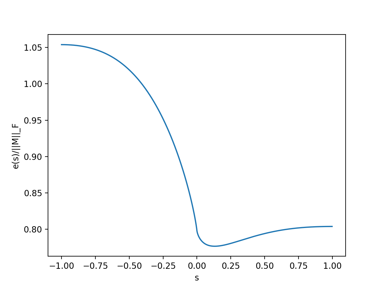
Fig. 1: Values of $\frac{e(s)}{\left\|M\right\|}_{F}$ when $s\in[-1,1]$.

Numerical experiment above shows that $\frac{e(s)}{\left\|M\right\|_{F}}\geq 0.77$ (hence $e(s)\geq 0.77$) for all $a\in[-1,1]$. Note that for each $i$, $Y_{i}:=\frac{\left|A_{i}MA_{i}^{T}\right|^{\frac{1}{2}}}{e(s)}-1$ is a centered sub-gaussian random variable. Hence, by (7.1) and (7.7),

$$\left\|Y_{i}\right\|_{\psi_{2}}\leq\sup_{p\geq 1}p^{-\frac{1}{2}}(\frac{2(\mathbb{E}|Z|^{p})^{\frac{1}{p}}}{e(s)}+1)\leq\frac{2}{0.77}\left\|Z\right\|_{\psi_{2}}+1<+\infty.$$

where $Z$ is a standard gaussian variable. Hence, (7.2) tells us that there exist universal constants $C>0$ and $c_{0}>0$ such that

$$\mathbb{P}\left(\left|\sum_{i=1}^{m}\left(\frac{\left|A_{i}MA_{i}^{T}\right|^{\frac{1}{2}}}{e(s)}-1\right)\right|>m\epsilon\right)\leq\hat{C}\exp(-\hat{c}_{0}m\epsilon^{2})$$ (7.9)

Consequently, for fixed $M$,

$$\frac{1}{m}\sum_{i=1}^{m}\left|A_{i}MA_{i}^{T}\right|^{\frac{1}{2}}\geq(1-\epsilon)e(s)\geq 0.77(1-\epsilon)\left\|M\right\|_{F}$$ (7.10)

holds with probability at least $1-\hat{C}\exp(-\hat{c}_{0}m\epsilon^{2})$.

Next we generalize (7.10) to all rank-2 matrices $M$. Again, by scale invariance, we assume $\left\|M\right\|_{F}=1$. Consequently, we only need to prove (9) holds with high probability for all $M\in\mathcal{M}:=\{\beta uu^{T}+\gamma vv^{T}|\left\|u\right\|=\left\|v\right\|=1$, $u^{T}v=0$ and $\beta^{2}+\gamma^{2}=1\}$. Set $\mathcal{S}_{\epsilon^{2}}:=\mathcal{T}_{\epsilon^{2}}\times\mathcal{N}_{\epsilon^{2}}\times\mathcal{N}_{\epsilon^{2}}$ where $\mathcal{T}_{\epsilon^{2}}$ is an $\epsilon^{2}$-net of $[-1,1]$ and $\mathcal{N}_{\epsilon^{2}}$ is an $\epsilon^{2}$-net of the unit sphere $\{x\in\mathbb{R}^{n}|\left\|x\right\|=1\}$. Since $|\mathcal{T}_{\epsilon^{2}}|\leq\frac{2}{\epsilon^{2}}$ and $|\mathcal{N}_{\epsilon^{2}}|\leq\left(\frac{3}{\epsilon^{2}}\right)^{n}$, we know $|\mathcal{S}_{\epsilon^{2}}|\leq\left(\frac{3}{\epsilon}\right)^{4n+2}$. Let $E$ denote the event that (7.10) holds for every $(\beta_{0},u_{0}.v_{0})\in\mathcal{S}_{\epsilon^{2}}$. Consequently,

$\mathbb{P}(E)\geq 1-2\hat{C}\left(\frac{3}{\epsilon}\right)^{4n+2}\exp(-\hat{c}_{0}m\epsilon^{2}).$

For $M\in\mathcal{M}$, we want to approximate $M=\beta uu^{T}+\gamma vv^{T}$ by an element $M_{0}=\beta_{0}u_{0}u_{0}^{T}+\gamma_{0}v_{0}v_{0}^{T}\in\mathcal{M}$ with $(\beta_{0},u_{0},v_{0})\in\mathcal{S}_{\epsilon^{2}}$. More precisely, let $(\beta_{0},u_{0},v_{0})\in\mathcal{S}_{\epsilon^{2}}$ and $M_{0}=\beta_{0}u_{0}u_{0}^{T}+\mathrm{sgn}(\gamma)\sqrt{1-\beta_{0}^{2}}v_{0}v_{0}^{T}$ be such that $|\beta-\beta_{0}|\leq\epsilon^{2}$, $\left\|u-u_{0}\right\|\leq\epsilon^{2}$ and $\left\|v-v_{0}\right\|\leq\epsilon^{2}$. Consequently, we have

$|\gamma-\mathrm{sgn}(\gamma)\sqrt{1-\beta_{0}^{2}}|=|\sqrt{1-\beta^{2}}-\sqrt{1-\beta_{0}^{2}}|\leq\left|\beta^{2}-\beta_{0}^{2}\right|^{\frac{1}{2}}\leq\sqrt{2}\left|\beta-\beta_{0}\right|^{\frac{1}{2}}\leq\sqrt{2}\epsilon.$

Also note that

$$\left\|\beta uu^{T}-\beta_{0}u_{0}u_{0}^{T}\right\|_{F} \leq|\beta-\beta_{0}|\left\|uu^{T}\right\|_{F}+\left\|\beta_{0}u(u-u_{0})^{T}\right\|_{F}+\left\|\beta_{0}(u-u_{0})u_{0}^{T}\right\|_{F}$$ (7.11)

$$=|\beta-\beta_{0}|\left\|u\right\|^{2}+|\beta_{0}|\left\|u-u_{0}\right\|(\left\|u\right\|+\left\|u_{0}\right\|)$$

$$\leq 3\epsilon^{2}<4\epsilon$$

Similarly we can prove $\left\|\gamma vv^{T}-\mathrm{sgn}(\gamma)\sqrt{1-\beta_{0}^{2}}v_{0}v_{0}^{T}\right\|\leq 2\epsilon^{2}+2\epsilon<4\epsilon$. On the intersection of events where (4.1) holds and $E$, we have

$$\left|\frac{1}{m}\sum_{i=1}^{m}|A_{i}MA_{i}^{T}|^{\frac{1}{2}}-\frac{1}{m}\sum_{i=1}^{m}|A_{i}M_{0}A_{i}^{T}|^{\frac{1}{2}}\right|\leq\frac{1}{m}\sum_{i=1}^{m}\left|\left|A_{i}MA_{i}^{T}\right|^{\frac{1}{2}}-\left|A_{i}M_{0}A_{i}^{T}\right|^{\frac{1}{2}}\right|$$

$$\leq\frac{1}{m}\sum_{i=1}^{m}\left|\left|A_{i}MA_{i}^{T}\right|-\left|A_{i}M_{0}A_{i}^{T}\right|\right|^{\frac{1}{2}}$$

$$\leq\left(\frac{1}{m}\sum_{i=1}^{m}\left|\left|A_{i}MA_{i}^{T}\right|-\left|A_{i}M_{0}A_{i}^{T}\right|\right|\right)^{\frac{1}{2}}$$

$$\leq\left(\frac{1}{m}\sum_{i=1}^{m}\left|A_{i}(M-M_{0})A_{i}^{T}\right|\right)^{\frac{1}{2}}$$

$$\leq\left(\frac{1}{m}\sum_{i=1}^{m}\left|A_{i}(\beta uu^{T}-\beta_{0}u_{0}u_{0}^{T})A_{i}^{T}\right|+\left|A_{i}(\gamma vv^{T}-\gamma_{0}v_{0}v_{0}^{T})A_{i}^{T}\right|\right)^{\frac{1}{2}}$$

$$\leq\left(\frac{1}{m}\sum_{i=1}^{m}\left|A_{i}(\beta uu^{T}-\beta_{0}u_{0}u_{0}^{T})A_{i}^{T}\right|\right)^{\frac{1}{2}}+\left(\frac{1}{m}\sum_{i=1}^{m}\left|A_{i}(\gamma vv^{T}-\gamma_{0}v_{0}v_{0}^{T})A_{i}^{T}\right|\right)^{\frac{1}{2}}$$

$$\leq 2^{\frac{1}{4}}(1+\epsilon)^{\frac{1}{2}}\left\|\beta uu^{T}-\beta_{0}u_{0}u_{0}^{T}\right\|_{F}^{\frac{1}{2}}+2^{\frac{1}{4}}(1+\epsilon)^{\frac{1}{2}}\left\|\gamma vv^{T}-\gamma_{0}v_{0}v_{0}^{T}\right\|_{F}^{\frac{1}{2}}$$

$$\leq 2^{\frac{9}{4}}(1+\epsilon)^{\frac{1}{2}}\epsilon^{\frac{1}{2}},$$

where the second inequality is by $||a|-|b||^{2}\leq|a^{2}-b^{2}|$ for any $a,b\in\mathbb{R}$, the third inequality is by concavity of $(\cdot)^{2}$, the fourth and the fifth inequalities are by triangle inequality, the sixth inequality is by $a^{2}+b^{2}\leq(a+b)^{2}$ for any $a,b\in\mathbb{R}$ and the seventh inequality is by the right hand side of equation (4.1). Consequently, if $m>c_{0}n\epsilon^{-2}\log\frac{1}{\epsilon}$

$$\frac{1}{m}\sum_{i=1}^{m}\left|A_{i}MA_{i}^{T}\right|^{\frac{1}{2}}\geq 0.77(1-\epsilon-2^{\frac{9}{4}}(1+\epsilon)^{\frac{1}{2}}\epsilon^{\frac{1}{2}})$$ (7.12)

holds with probability at least $1-2\hat{C}\left(\frac{3}{\epsilon}\right)^{4n+2}\exp(-\hat{c}_{0}m\epsilon^{2})-C\exp(-c_{1}\epsilon^{2}m)$. As in (7.5), by making $c_{0}$ large, we are able to make the probability $\geq 1-\hat{\hat{C}}\exp(-\hat{\hat{c}}_{0}m\epsilon^{2})$ for some constants $\hat{\hat{C}}$ and $\hat{\hat{c}}_{0}$. By letting $\tilde{\epsilon}:=\epsilon+2^{\frac{9}{4}}(1+\epsilon)^{\frac{1}{2}}\epsilon^{\frac{1}{2}}$ and adjust constants $\hat{\hat{C}},\hat{\hat{c}}_{0},c_{0}$ we arrive at the desired result. $\square$

Proof of Lemma 10: If $x=0$ or $y=0$ or $x=y$, the inequality holds. Thus, in particular, by the symmetry of (4.6) in $x$ and $y$, we can assume that $\left\|x\right\|\geq\left\|y\right\|>0$. Dividing (4.6) by $\left\|x\right\|$, tells us that we can assume $\left\|x\right\|=1$ and $\left\|y\right\|=t$ for $t\in[0,1]$. Set $\rho:=\frac{x^{T}y}{\left\|y\right\|}\in[0,1]$, and define $h(t,\rho):=\sqrt{t^{2}-2\rho t+1}+\sqrt{t^{2}+2\rho t+1}-1-t=\left\|x+y\right\|+\left\|x-y\right\|-\left\|x\right\|-\left\|y\right\|$. If $x=y$, we are done; otherwise, set $q(t,\rho):=\frac{h(t,\rho)}{\sqrt{t^{2}-2\rho t+1}}=\frac{\left\|x+y\right\|+\left\|x-y\right\|-\left\|x\right\|-\left\|y\right\|}{\left\|x-y\right\|}$, for each $(t,\rho)\in[0,1]\times[0,1]$. We now show that the minimum value of $q$ over $[0,1]\times[0,1]$ is $2-\sqrt{2}$. For fixed $t\in[0,1]$,

$$\frac{\partial q(t,\rho)}{\partial\rho} =\frac{t(t^{2}+1)}{(t^{2}-2\rho t+1)^{\frac{3}{2}}}\left[\frac{2}{(t^{2}+2\rho t+1)^{\frac{1}{2}}}-\frac{t+1}{t^{2}+1}\right]$$

$$\geq\frac{t(t^{2}+1)}{(t^{2}-2\rho t+1)^{\frac{3}{2}}}\left[\frac{2}{t+1}-\frac{t+1}{t^{2}+1}\right]$$

$$\geq 0,$$

where the first inequality follows since $t^{2}+2\rho t+1\leq(1+t)^{2}$ as $\rho\in[0,1]$, and the last inequality follows since $2(t^{2}+1)\geq(t+1)^{2}$. That is, $q(t,\rho)$ is increasing with respect to $\rho$ when $\rho\in[0,1]$ for each fixed $t\in[0,1]$. Also

$$\frac{dq(t,0)}{dt}=-\frac{1-t}{(1+t^{2})^{\frac{3}{2}}}\leq 0.$$

Hence $q(t,0)$ is decreasing for $t\in[0,1]$. We know for each $t\in[0,1]$, $\rho\in[0,1]$,

$$q(t,\rho)\geq q(t,0)\geq q(1,0)=2-\sqrt{2}$$

Thus $h(t,\rho)\geq(2-\sqrt{2})\left\|x-y\right\|$, which leads to the desired result. $\square$

Proof of Lemma 11: If $x=y=0$, we are done. Next assume at least one of $x$ and $y$ is non-zero. We assume $\left\|x\right\|=1$ and $\left\|y\right\|=t\in[0,1]$ since we can divide (4.7) by $\max\{\left\|x\right\|,\left\|y\right\|\}$ on both sides. Set $\rho:=\frac{x^{T}y}{\left\|y\right\|}$. We have

$$\sqrt{2}\left\|xx^{T}-yy^{T}\right\|_{F} \!=\!\sqrt{2}\left(\sum_{i,j}(x_{i}x_{j}-y_{i}y_{j})^{2}\right)^{\frac{1}{2}}$$

$$\!=\!\sqrt{2}\left(\!(\sum_{i}x_{i}^{2})(\sum_{j}x_{j}^{2})\!+\!(\sum_{i}y_{i}^{2})(\sum_{j}y_{j}^{2})\!-\!2(\sum_{i}x_{i}y_{i})(\sum_{j}x_{j}y_{j})\!\right)^{\frac{1}{2}}$$

$$\!=\!\left(2(1+t^{4})-4\rho^{2}t^{2}\right)^{\frac{1}{2}}$$

$$\!\geq\!\left((1+t^{2})^{2}-4\rho^{2}t^{2}\right)^{\frac{1}{2}}$$

$$\!=\!\sqrt{1+t^{2}+2\rho t}\sqrt{1+t^{2}-2\rho t}$$

$$\!=\!\left\|x+y\right\|\left\|x-y\right\|,$$

where the inequality follows by the algebraic geometric mean inequality. $\square$

References

- [1] Aleksandr Aravkin, James V Burke, and Daiwei He. Iteratively re-weighted least squares for non-convex optimization. Technical report, University of Washington, Preprint, 2019.
- [2] Radu Balan, Pete Casazza, and Dan Edidin. On signal reconstruction without phase. Applied and Computational Harmonic Analysis, 20(3):345–356, 2006.
- [3] Richard Baraniuk, Mark Davenport, Ronald DeVore, and Michael Wakin. A simple proof of the restricted isometry property for random matrices. Constructive Approximation, 28(3):253–263, 2008.
- [4] James Burke and Sien Deng. Weak sharp minima revisited part i: basic theory. Control and Cybernetics, 31:439–469, 2002.
- [5] James V Burke. Descent methods for composite nondifferentiable optimization problems. Mathematical Programming, 33(3):260–279, 1985.
- [6] James V Burke and Sien Deng. Weak sharp minima revisited, part ii: application to linear regularity and error bounds. Mathematical programming, 104(2-3):235–261, 2005.
- [7] James V Burke and Sien Deng. Weak sharp minima revisited, part iii: Error bounds for differentiable convex inclusions. Mathematical Programming, 116(1-2):37–56, 2009.
- [8] James V Burke and Michael C Ferris. Weak sharp minima in mathematical programming. SIAM Journal on Control and Optimization, 31(5):1340–1359, 1993.
- [9] Emmanuel J Candes. The restricted isometry property and its implications for compressed sensing. Comptes rendus mathematique, 346(9-10):589–592, 2008.
- [10] Emmanuel J Candès and Xiaodong Li. Solving quadratic equations via phaselift when there are about as many equations as unknowns. Foundations of Computational Mathematics, 14(5):1017–1026, 2014.
- [11] Emmanuel J Candes, Xiaodong Li, and Mahdi Soltanolkotabi. Phase retrieval via wirtinger flow: Theory and algorithms. IEEE Transactions on Information Theory, 61(4):1985–2007, 2015.
- [12] Emmanuel J Candes, Thomas Strohmer, and Vladislav Voroninski. Phaselift: Exact and stable signal recovery from magnitude measurements via convex programming. Communications on Pure and Applied Mathematics, 66(8):1241–1274, 2013.
- [13] Emmanuel J Candès and Terence Tao. Decoding by linear programming. IEEE Transactions on Information Theory, 51(12):4203–4215, 2005.
- [14] Emmanuel J Candes and Terence Tao. Near-optimal signal recovery from random projections: Universal encoding strategies? IEEE Transactions on Information Theory, 52(12):5406–5425, 2006.
- [15] Vasileios Charisopoulos, Yudong Chen, Damek Davis, Mateo Díaz, Lijun Ding, and Dmitriy Drusvyatskiy. Low-rank matrix recovery with composite optimization: good conditioning and rapid convergence. arXiv preprint arXiv:1904.10020, 2019.
- [16] Jinghui Chen, Lingxiao Wang, Xiao Zhang, and Quanquan Gu. Robust wirtinger flow for phase retrieval with arbitrary corruption. arXiv preprint arXiv:1704.06256, 2017.
- [17] Yuxin Chen and Emmanuel Candes. Solving random quadratic systems of equations is nearly as easy as solving linear systems. In Advances in Neural Information Processing Systems, pages 739–747, 2015.
- [18] Albert Cohen, Wolfgang Dahmen, and Ronald DeVore. Compressed sensing and best 𝑘-term approximation. Journal of the American mathematical society, 22(1):211–231, 2009.
- [19] Ingrid Daubechies, Ronald DeVore, Massimo Fornasier, and C Sinan Güntürk. Iteratively reweighted least squares minimization for sparse recovery. Communications on Pure and Applied Mathematics: A Journal Issued by the Courant Institute of Mathematical Sciences, 63(1):1–38, 2010.
- [20] Damek Davis, Dmitriy Drusvyatskiy, and Courtney Paquette. The nonsmooth landscape of phase retrieval. arXiv preprint arXiv:1711.03247, 2017.
- [21] Laurent Demanet and Paul Hand. Stable optimizationless recovery from phaseless linear measurements. Journal of Fourier Analysis and Applications, 20(1):199–221, 2014.
- [22] David L Donoho et al. Compressed sensing. IEEE Transactions on information theory, 52(4):1289–1306, 2006.
- [23] David L Donoho and Xiaoming Huo. Uncertainty principles and ideal atomic decomposition. IEEE transactions on information theory, 47(7):2845–2862, 2001.
- [24] John C Duchi and Feng Ruan. Solving (most) of a set of quadratic equalities: Composite optimization for robust phase retrieval. arXiv preprint arXiv:1705.02356, 2017.
- [25] Rémi Gribonval and Morten Nielsen. Sparse representations in unions of bases. PhD thesis, INRIA, 2002.
- [26] Xiaodong Li and Vladislav Voroninski. Sparse signal recovery from quadratic measurements via convex programming. SIAM Journal on Mathematical Analysis, 45(5):3019–3033, 2013.
- [27] D Russell Luke, James V Burke, and Richard G Lyon. Optical wavefront reconstruction: Theory and numerical methods. SIAM review, 44(2):169–224, 2002.
- [28] Panos M Pardalos and Stephen A Vavasis. Quadratic programming with one negative eigenvalue is np-hard. Journal of Global Optimization, 1(1):15–22, 1991.
- [29] Mark Rudelson and Roman Vershynin. On sparse reconstruction from fourier and gaussian measurements. Communications on Pure and Applied Mathematics: A Journal Issued by the Courant Institute of Mathematical Sciences, 61(8):1025–1045, 2008.
- [30] Roman Vershynin. Introduction to the non-asymptotic analysis of random matrices. arXiv preprint arXiv:1011.3027, 2010.
- [31] Irène Waldspurger, Alexandre d’Aspremont, and Stéphane Mallat. Phase recovery, maxcut and complex semidefinite programming. Mathematical Programming, 149(1-2):47–81, 2015.
- [32] Gang Wang, Georgios B Giannakis, and Yonina C Eldar. Solving systems of random quadratic equations via truncated amplitude flow. IEEE Transactions on Information Theory, 64(2):773–794, 2018.
- [33] Huishuai Zhang, Yuejie Chi, and Yingbin Liang. Provable non-convex phase retrieval with outliers: Median truncatedwirtinger flow. In International conference on machine learning, pages 1022–1031, 2016.
- [34] Peng Zheng and Aleksandr Aravkin. Relax-and-split method for nonsmooth nonconvex problems. arXiv preprint arXiv:1802.02654, 2018.