Factor Models for High-Dimensional Functional Time Series

Abstract

In this paper, we set up the theoretical foundations for a high-dimensional functional factor model approach in the analysis of large cross-sections (panels) of functional time series (FTS). We first establish a representation result stating that, under mild assumptions on the covariance operator of the cross-section, we can represent each FTS as the sum of a common component driven by scalar factors loaded via functional loadings, and a mildly cross-correlated idiosyncratic component. Our model and theory are developed in a general Hilbert space setting that allows for mixed panels of functional and scalar time series. We then turn to the identification of the number of factors, and the estimation of the factors, their loadings, and the common components. We provide a family of information criteria for identifying the number of factors, and prove their consistency. We provide average error bounds for the estimators of the factors, loadings, and common component; our results encompass the scalar case, for which they reproduce and extend, under weaker conditions, well-established similar results. Under slightly stronger assumptions, we also provide uniform bounds for the estimators of factors, loadings, and common component, thus extending existing scalar results. Our consistency results in the asymptotic regime where the number $N$ of series and the number $T$ of time observations diverge thus extend to the functional context the “blessing of dimensionality” that explains the success of factor models in the analysis of high-dimensional (scalar) time series. We provide numerical illustrations that corroborate the convergence rates predicted by the theory, and provide finer understanding of the interplay between $N$ and $T$ for estimation purposes. We conclude with an application to forecasting mortality curves, where we demonstrate that our approach outperforms existing methods.

Keywords:

Functional time series, High-dimensional time series, Factor model, Panel Data, Functional data analysis.

MSC 2010 subject classification:

62H25, 62M10, 60G10.

1 Introduction

Throughout the last decades, researchers have been dealing with datasets of increasing size and complexity. In particular, Functional Data Analysis (see e.g. Ramsay & Silverman, 2005; Ferraty & Vieu, 2006; Horváth & Kokoszka, 2012; Hsing & Eubank, 2015; Wang et al., 2015) has received much interest and, in view of its relevance in a number of applications, has gained fast-growing popularity. In Functional Data Analysis, the observations are taking values in some functional space, usually some Hilbert space $H$—often, in practice, the space ${{L^{2}\left([0,1],\mathbb{R}\right)}}$ of real-valued squared-integrable functions. When an ordered sequence of functional observations exhibits serial dependence, we enter the realm of Functional Time Series (FTS) (Hörmann & Kokoszka, 2010, 2012). Many standard univariate and low-dimensional multivariate time-series methods have been adapted to this functional setting, either using a time-domain approach (Kokoszka & Reimherr, 2013a, b; Hörmann et al., 2013; Aue et al., 2014, 2015; Horváth et al., 2014; Aue et al., 2017; Górecki, Hörmann, Horváth & Kokoszka, 2018; Bücher et al., 2020; Gao et al., 2018), a frequency domain approach under stationarity assumptions (Panaretos & Tavakoli, 2013a, b; Hörmann et al., 2015; Tavakoli & Panaretos, 2016; Hörmann et al., 2018; Rubín & Panaretos, 2020; Fang et al., 2020) or under local stationarity assumptions (van Delft et al., 2017; van Delft & Eichler, 2018; van Delft & Dette, 2021).

Parallel to this development of functional time series analysis, data in high dimensions (e.g. Bühlmann & van de Geer, 2011; Fan et al., 2013) have become pervasive in data sciences and related disciplines where, under the name of Big Data, they constitute one of the most active subjects of contemporary statistical research.

This contribution stands at the intersection of these two strands of literature, cumulating the challenges of function-valued observations and those of high dimension. Datasets, in this context, consist of large collections of $N$ scalar or functional time series—equivalently, scalar or functional time series in high dimension (from fifty, say, to several hundreds)—observed over a period of time $T$. Typical examples are continuous-time series of concentrations for a large number of pollutants, or/and collected daily over a large number of sites, daily series of returns observed at high intraday frequency for a large collection of stocks, or intraday energy consumption curves, to name only a few. Not all component series in the dataset are required to be function-valued, though, and it is very important for practice that mixed panels of scalar and functional series can be considered as well. In order to model such datasets, we develop a class of high-dimensional functional factor models inspired by the factor model approaches developed, mostly, in time series econometrics, which have proven effective, flexible, and quite efficient in the scalar case.

Since the econometric literature may be unfamilar to much of the readership of this journal, a general presentation of factor model methods for high-dimensional time series is in order. The basic idea of the approach consists of decomposing the observation into the sum of two mutually orthogonal unobserved components: the common component, a reduced-rank process driven by a small number of common shocks which account for most of the cross-correlations, and the idiosyncratic component which, consequently, is only mildly cross-correlated. Early instances of this can be traced back to the pioneering contributions by Geweke (1977), Sargent & Sims (1977), Chamberlain (1983), and Chamberlain & Rothschild (1983). The factor models considered by Geweke, Sargent, and Sims are exact, that is, involve mutually orthogonal (all leads, all lags) idiosyncratic components; the common shocks then account for all cross-covariances, a most restrictive assumption that cannot be expected to hold in practice. Chamberlain (1983) and Chamberlain & Rothschild (1983) are relaxing this exactness assumption into an assumption of mildly cross-correlated idiosyncratics (the so-called “approximate factor models”).Finite-$N$ non-identifiability is the price to be paid for that relaxation; the resulting models, however, remain asymptotically (as $N$ tends to infinity) identified, which is perfectly in line with the spirit of high-dimensional asymptotics.

This idea of an approximate factor model in the analysis of high-dimensional time series has been picked up, and popularized in the early 2000s, mostly by Stock & Watson (2002a, b); Bai & Ng (2002); Bai (2003), and Forni et al. (2000), followed by many others. The most common definition of “mildly cross-correlated,” hence of “idiosyncratic,” is “a (second-order stationary) process $\{\xi_{it}\,|\,i\in\mathbb{N},\,t\in\mathbb{Z}\}$ is called idiosyncratic if the variance of any sequence of normed (sum of squared coefficients equal to one) linear combination of the present, past, and future values of $\{\xi_{it}\}$, $i=1,\ldots,N$ is bounded as $N\to\infty$.” With this definition, Hallin & Lippi (2013) show that, under very general regularity assumptions, the decomposition into common and idiosyncratic constitutes a representation result rather than a statistical model—meaning that (at population level) it exists and is fully identified—and coincides with the so-called general(ized) dynamic factor model of Forni et al. (2000).

Let us give some intuition for common and idiosyncratic components for scalar data. In finance and economics, the common component is the co-movement of all the series, which are highly cross-sectionally correlated, and the idiosyncratic is thus literally the individual movement of each component that has smaller correlations with others. For financial data, low common-to-idiosyncratic variance ratios are typical for each series. However, not matter how small the values of these ratios, the contribution of the idiosyncratics, as $N\to\infty$, is eventually surpassed by that of the common component due to the pervasiveness of the factors (co-movements).

Most existing factor models then can be obtained by imposing further restrictions on this representation result: assuming a finite-dimensional common space yields the models proposed by Stock & Watson (2002a, b) and Bai & Ng (2002), additional sparse covariance assumptions characterize the approaches by Fan et al. (2011, 2013), and the dimension-reduction approach by Lam et al. (2011) and Lam & Yao (2012) is based on the assumption of i.i.d. idiosyncratic components. For further references on dynamic factor models, we refer to the survey paper by Bai & Ng (2008) or the monographs by Stock & Watson (2011) and Hallin et al. (2020); for the state-of-the-art on general dynamic factor models, see Forni et al. (2015, 2017).

Factor models for univariate functional data have already been studied: these are based on models which consider functional factors with scalar loadings (Hays et al., 2012; Kokoszka et al., 2015; Young, 2016; Bardsley et al., 2017; Kokoszka et al., 2017; Horváth et al., 2020), scalar factors with functional loadings (Kokoszka et al., 2018), functional factors with loadings that are operators (Tian, 2020), or scalar factors and loadings in a smoothing model (Gao et al., 2021).

For multivariate functional data (moderate fixed dimension), the only factor models we are aware of were introduced by Castellanos et al. (2015), who consider a multivariate Gaussian factor model with functional factors and scalar loadings, by Kowal et al. (2017), with scalar factors and functional loadings within a dynamic linear model, and by White & Gelfand (2020) with functional factors and scalar loadings within a multi-level model. There exists, also, a substantial literature on modelling multivariate functional data, see for instance Happ & Greven (2018); Górecki, Krzyśko, Waszak & Wołyński (2018); Wong et al. (2019); Li et al. (2020); Zhang et al. (2020); Qiu et al. (2021). Except for Wong et al. (2019), all these contributions, however, are limited to fixed-dimension vectors of functional data defined on the same domain.

The increasing availability of high-dimensional FTS data, requiring high-dimensional asymptotics under which the dimension of the functional objects is diverging with the sample size, recently has generated much interest: Zhou & Dette (2020) consider statistical inference for sums of high-dimensional FTS, Fang et al. (2020) explore new perspectives on dependence for high-dimentional FTS, Chang et al. (2020) study a learning framework based on autocovariances, and Hu & Yao (2021) investigate a sparse functional principal component analysis in high dimensions under Gaussian assumptions. Again, all functional components involved, in these papers, are required to take values in the same functional space.

On the other hand, the factor model approach in the statistical analysis of high-dimensional FTS remains largely unexplored. Gao et al. (2018) are using factor model techniques in the forecasting of high-dimensional FTS. They adopt a heuristic two-stage approach combining a truncated-PCA dimension reduction and separate scalar factor-model analyses of the resulting (scalar) panels of scores.

Our approach, inspired by the time-series econometrics literature, is radically different. Indeed, we start (Section 2.3) with a stochastic representation result establishing the existence, under a functional version of the traditional assumptions on dynamic panels, of a factor model representation of the observations with scalar factors and functional loadings. Theorems 2.2 and 2.3 are relating the existence and the form of a high-dimensional functional factor model representation to the asymptotic behavior of the eigenvalues of the panel covariance operator of the observations; they actually are the functional counterparts of classical results by Chamberlain & Rothschild (1983) and Chamberlain (1983). Contrary to Gao et al. (2018), our approach, thus, is principled: the existence and the form of our factor model representation are neither an assumption nor the description of a presupposed data-generating process but follow from a mathematical result. It avoids the loss of information related with Gao et al.’s truncation of the PCA decomposition and their separate analysis of interrelated panels of principal component scores. Its scalar factors and functional loadings, moreover, allow for the analysis of panels comprising time series of different types, functional and scalar.

Drawing inspiration from Stock & Watson (2002a), Stock & Watson (2002b), and Bai & Ng (2002), we then develop an estimation theory for the unobserved factors, loadings, and common components (Theorems 4.3, 4.4, 4.6, and 4.7). This is laying the theoretical foundations for an analysis of high-dimensional FTS. Since our methods can deal with mixed panels of scalar and functional time series, our results encompass and extend, sometimes under weaker assumptions, the classical ones by Chamberlain & Rothschild (1983); Bai & Ng (2002); Stock & Watson (2002a); Fan et al. (2013).

Our paper also derives a forecasting method for high-dimensional FTS. Through a panel of Japanese mortality curves, we show the superior accuracy of our method compared to alternative forecasting methods.

The paper is organized as follows. Section 2 is devoted to our representation result: roughly, a factor-model representation, with $r$ scalar factors and functional loadings, exists if and only if the number of diverging (as $N\to\infty$) eigenvalues of the covariance operator of the $N$-dimensional observation is $r$. Section 3 is dealing with estimation procedures: Section 3.1 introduces our estimators of the factors, loadings, and common component through a least squares approach and Section 3.2 provides a family of criteria for the identification of the number $r$ of factors. Section 4 is about the consistency properties of the procedures described in Section 3: consistency (Section 4.1) of the identification method of Section 3.2 and consistency rate results for the estimators described in Section 3.1. The latter take the form of average (Section 4.2) and uniform (Section  4.3) error bounds, respectively. In Section 5, we conduct some numerical experiments, and provide the forecasting application in Section 6. We conclude in Section 7 with a discussion. Technical results and all the proofs, as well as additional simulation results, are contained in the Appendices.

2 A representation Theorem

2.1 Notation

Throughout, we denote by

(2.1) $${\cal X}_{N,T}\vcentcolon=\{x_{it},\ i=1,\ldots,N,\;t=1,\ldots,T\}\quad N\in\mathbb{N},\ T\in\mathbb{N}$$

an observed $N\times T$ panel of time series, where the random elements $\{x_{it}:t\geq 1\}$ take values in a real separable Hilbert space $H_{i}$ equipped with the inner product $\left\langle\cdot,\cdot\right\rangle_{H_{i}}$ and norm ${\left\lVert\cdot\right\rVert}_{H_{i}}\vcentcolon=\left\langle\cdot,\cdot\right\rangle_{H_{i}}^{1/2}$, $i=1,\ldots,N$. These series can be of different types. A case of interest is the one for which some series are scalar ($H_{i}=\mathbb{R}$) and some others are square-integrable functions from some closed real interval to $\mathbb{R}$, that is, $H_{i}=L^{2}([a_{i},b_{i}],\mathbb{R}),$ where $a_{i},b_{i}\in\mathbb{R}$ with $a_{i}<b_{i}$. The typical inner-product on $L^{2}([a_{i},b_{i}],\mathbb{R})$ is $\left\langle f,g\right\rangle_{H_{i}}\vcentcolon=\int_{a_{i}}^{b_{i}}f(\tau)g(\tau)d\tau$ for $f,g\in L^{2}([a_{i},b_{i}],\mathbb{R})$. While the results could be derived for these special cases only, the generality of our approach allows the practitioner to choose the Hilbert spaces $H_{1},\ldots,H_{N}$ to suit their specific application.

We tacitly assume that all $x_{it}$’s are random elements with mean zero and finite second-order moments defined on some common probability space $(\Omega,\mathcal{F},\operatorname{{\mathbb{P}}})$; we also assume that ${\cal X}_{N,T}$ constitutes the finite realization of some second-order $t$-stationary double-indexed process ${\cal X}\vcentcolon=\{x_{it},\ i\in\mathbb{N},\;t\in\mathbb{Z}\}$. The mean zero assumption is not necessary, but simplifies the exposition—See Section E of the Appendices for more general, non zero-mean results. In practice, each observed series $\{x_{it}\}$ is centered at its empirical mean at the start of the statistical analysis.

Define ${\bm{H}}_{N}\vcentcolon=H_{1}{\scriptstyle\bigoplus}H_{2}{\scriptstyle\bigoplus}\cdots{\scriptstyle\bigoplus}H_{N}$ as the (orthogonal) direct sum of the Hilbert spaces $H_{1},\ldots,H_{N}$. The elements of ${\bm{H}}_{N}$ are of the form $\bm{v}\vcentcolon=(v_{1},v_{2},\ldots,v_{N})^{\mathsf{T}}$ or $\bm{w}\vcentcolon=(w_{1},w_{2},\ldots,w_{N})^{\mathsf{T}}$, where $v_{i},w_{i}\in H_{i},i=1,\ldots,N$, and $\cdot^{\mathsf{T}}$ denotes transposition. The $i$-th component of an element of ${\bm{H}}_{N}$ is denoted by $(\cdot)_{i}$; for instance, $({\bm{v}})_{i}$ stands for $v_{i}$. The space ${\bm{H}}_{N}$, naturally equipped with the inner product

$$\left\langle\bm{v},\bm{w}\right\rangle_{{\bm{H}}_{N}}\vcentcolon=\sum_{i=1}^{N}\left\langle v_{i},w_{i}\right\rangle_{H_{i}},$$

is a real separable Hilbert space. When no confusion is possible, we write $\left\langle\cdot,\cdot\right\rangle$ for $\left\langle\cdot,\cdot\right\rangle_{{\bm{H}}_{N}}$ and ${\left\lVert\cdot\right\rVert}\vcentcolon={\left\langle\cdot,\cdot\right\rangle}^{1/2}$ for the resulting norm. Let $\mathcal{L}(H_{1},H_{2})$ denote the space of bounded (linear) operators from $H_{1}$ to $H_{2}$, and use the shorthand notation $\mathcal{L}(H)$ for $\mathcal{L}(H,H)$. Denote the operator norm of $V\in\mathcal{L}(H_{1},H_{2})$ by

$${\left|\kern-0.86108pt\left|\kern-0.86108pt\left|V\right|\kern-0.86108pt\right|\kern-0.86108pt\right|}_{\infty}\vcentcolon=\sup_{x\in H_{1},x\neq 0}{\left\lVert Vx\right\rVert}_{H_{2}}/{\left\lVert x\right\rVert}_{H_{1}},$$

and write $V^{\star}$ for the adjoint of $V$, which satisfies $\left\langle Vu_{1},u_{2}\right\rangle_{H_{2}}=\left\langle u_{1},V^{\star}u_{2}\right\rangle_{H_{1}}$ for all $u_{1}\in\leavevmode\nobreak\ \!H_{1}$ and $u_{2}\in H_{2}$. In particular, we have

$${\left|\kern-0.86108pt\left|\kern-0.86108pt\left|V\right|\kern-0.86108pt\right|\kern-0.86108pt\right|}_{\infty}={\left|\kern-0.86108pt\left|\kern-0.86108pt\left|V^{\star}\right|\kern-0.86108pt\right|\kern-0.86108pt\right|}_{\infty}={\left|\kern-0.86108pt\left|\kern-0.86108pt\left|V^{\star}V\right|\kern-0.86108pt\right|\kern-0.86108pt\right|}_{\infty}^{1/2},$$

see Hsing & Eubank (2015). We denote by ${\left|\kern-0.86108pt\left|\kern-0.86108pt\left|V\right|\kern-0.86108pt\right|\kern-0.86108pt\right|}_{2}$ the Hilbert–Schmidt norm of an operator $V\in\mathcal{S}_{\infty}(H_{1},H_{2})$ defined by ${\left|\kern-0.86108pt\left|\kern-0.86108pt\left|V\right|\kern-0.86108pt\right|\kern-0.86108pt\right|}_{2}\vcentcolon=\big{[}\sum_{j\geq 1}{\left\lVert Ve_{i}\right\rVert}_{H_{2}}^{2}\big{]}^{1/2}$ where $\{e_{i}\}\subset H_{1}$ is an orthonormal basis of $H_{1}$, the sum might be finite or infinite, and is independent of the choice of the basis. If $V\in\mathbb{R}^{p\times q}$, then the Hilbert–Schmidt norm is often called the Frobenius norm. For $u_{1}\in H_{1},u_{2}\in H_{2}$, define $u_{1}\operatorname*{\otimes}u_{2}\in\mathcal{L}(H_{2},H_{1})$ by $(u_{1}\operatorname*{\otimes}u_{2})(v_{2})=\left\langle u_{2},v_{2}\right\rangle_{H_{2}}u_{1}$ for all $v_{2}\in H_{2}$. If $\alpha\in\mathbb{R},u\in H$, we define $u\alpha\vcentcolon=\alpha u$. We shall denote by $\mathbb{R}^{p\times q}$ the space of $p\times q$ real matrices, and will identify this space with the space of mappings $\mathcal{L}(\mathbb{R}^{q},\mathbb{R}^{p})$. Notice that for $\bm{A}\in\mathbb{R}^{p\times q}$, $\bm{A}^{\mathsf{T}}=\bm{A}^{\star}$. We write $\mathbb{N}$ for the set of positive integers, that is, $\mathbb{N}\vcentcolon=\{1,2,\ldots\}$, and denote the Euclidean norm in $\mathbb{R}^{p}$ by ${\left|\cdot\right|}$.

When working with the panel data, let ${\bm{x}}_{t}\vcentcolon=(x_{1t},x_{2t},\ldots,x_{Nt})^{\mathsf{T}}\leavevmode\nobreak\ \!\in\leavevmode\nobreak\ \!\bm{H}_{N}$ where, in order to keep the presentation simple, the dependence on $N$ does not explicitly appear. We denote by $\lambda_{N,1}^{x},\lambda_{N,2}^{x},\ldots$ the eigenvalues, in decreasing order of magnitude, of ${\bm{x}}_{t}$’s covariance operator ${\mathbb{E}\left[({\bm{x}}_{t}-\operatorname{\>{\mathbb{E}}}{\bm{x}}_{t})\operatorname*{\otimes}({\bm{x}}_{t}-\operatorname{\>{\mathbb{E}}}{\bm{x}}_{t})\right]}\in\mathcal{L}({\bm{H}}_{N})$, which maps ${\bm{y}}\in{\bm{H}}_{N}$ to

$${\mathbb{E}\left[\left\langle{\bm{x}}_{t}-\operatorname{\>{\mathbb{E}}}{\bm{x}}_{t},{\bm{y}}\right\rangle({\bm{x}}_{t}-\operatorname{\>{\mathbb{E}}}{\bm{x}}_{t})\right]}\in{\bm{H}}_{N},$$

(Hsing & Eubank, 2015, Definition 7.2.3). In view of stationarity, these eigenvalues do not depend on $t$. Unless otherwise mentioned, convergence of sequences of random variables is in mean square.

2.2 A functional factor model

The basic idea in all factor-model approaches to the analysis of high-dimensional time series consists in decomposing the observation $x_{it}$ into the sum $\chi_{it}+\xi_{it}$ of two unobservable and mutually orthogonal components, the common component $\chi_{it}$ and the idiosyncratic one $\xi_{it}$. The various factor models that are found in the literature only differ in the way $\chi_{it}$ and $\xi_{it}$ are characterized. The characterization we are adopting here is inspired from Forni & Lippi (2001).

Definition 2.1.

The functional zero-mean second-order stationary stochastic process

$${\cal X}\vcentcolon=\{x_{it}:\,i\in\leavevmode\nobreak\ \!\mathbb{N},\;t\in\leavevmode\nobreak\ \!\mathbb{Z}\}$$

admits a (high-dimensional) functional factor model representation with $r\in\mathbb{N}$ factors if there exist loadings $b_{il}\in H_{i}$, $i\in\mathbb{N}$, $l=1,\ldots,r$, $H_{i}$-valued processes $\{\xi_{it}:\ t\in\mathbb{Z}\}$, $i\in\mathbb{N}$, and a real $r$-dimensional second-order stationary process $\{{\bm{u}}_{t}=(u_{1t},\ldots,u_{rt})^{\mathsf{T}}:\ t\in\mathbb{Z}\}$, co-stationary with $\mathcal{X}$, such that

(2.2) $$x_{it}=\chi_{it}+\xi_{it}=b_{i1}u_{1t}+b_{i2}u_{2t}+\cdots+b_{ir}u_{rt}+\xi_{it},\qquad i\in\mathbb{N},\>\>t\in\mathbb{Z}$$

($\chi_{it}$ and $\xi_{it}$ unobservable) holds with

1. $\operatorname{\>{\mathbb{E}}}{{\bm{u}}}_{t}={\bm{0}}$ and ${\mathbb{E}\left[{{\bm{u}}}_{t}{{\bm{u}}}^{\mathsf{T}}_{t}\,\right]}=\bm{\Sigma}_{\bm{u}}\in\mathbb{R}^{r\times r}$ is positive definite;

2. ${\mathbb{E}\left[u_{lt}\xi_{it}\right]}=0$ and ${\mathbb{E}\left[\xi_{it}\right]}=0$ for all $t\in\mathbb{Z}$, $l=1,\ldots,r$, and $i\in\mathbb{N}$;

3. denoting by $\lambda^{\xi}_{N,l}$ the $l$-th (in decreasing order of magnitude) eigenvalue of the covariance operator ${\mathbb{E}\left[{\bm{\xi}}_{t}\operatorname*{\otimes}{\bm{\xi}}_{t}\right]}$ of $\bm{\xi}_{t}\!\vcentcolon=(\xi_{1t},\ldots,\xi_{Nt})^{\mathsf{T}}$, $\lambda^{\xi}_{1}\!\vcentcolon=\sup_{N}\lambda^{\xi}_{N,1}\leavevmode\nobreak\ \!\!<\leavevmode\nobreak\ \!\infty$;

4. denoting by $\lambda^{\chi}_{N,l}$ the $l$-th (in decreasing order of magnitude) eigenvalue of the covariance operator ${\mathbb{E}\left[{\bm{\chi}}_{t}\operatorname*{\otimes}{\bm{\chi}}_{t}\right]}$ of $\bm{\chi}_{t}\!\vcentcolon=(\chi_{1t},\ldots,\chi_{Nt})^{\mathsf{T}}\!\!$, $\lambda^{\chi}_{r}\vcentcolon=\sup_{N}\lambda^{\chi}_{N,r}\!\leavevmode\nobreak\ \!=\leavevmode\nobreak\ \!\infty$.

The $r$ scalar random variables $u_{lt}$ are called factors; the $b_{il}$’s are the (functional) factor loadings; $\chi_{it}$ and $\xi_{it}$ are called $x_{it}$’s common and idiosyncratic component, respectively.

Notice that the number $r\in\mathbb{N}$ is crucial in this definition, which calls for some remarks and comments.

1. In the terminology of Hallin & Lippi (2013), equation (2.2), where the factors are loaded contemporaneously, is a static functional factor representation, as opposed to the general dynamic factor representation, where the $b_{ij}$’s are linear one-sided square-summable filters of the form $b_{ij}(L)=\sum_{k=0}^{\infty}b_{ijk}L^{k}$ ($L$ the lag operator), and the $u_{jt}$’s are mutually orthogonal second-order white noises (the common shocks) satisfying ${\mathbb{E}\left[u_{lt}\xi_{is}\right]}=0$ for all $t,s\in\mathbb{Z}$ and $l=1,\ldots,r$. The static $r$-factor model where the $r$ factors are driven by $q\leq r$ shocks is a particular case of the general dynamic one with $q\leq r$ common shocks. When the idiosyncratic processes $\{\xi_{it}:\ t\leavevmode\nobreak\ \!\in\leavevmode\nobreak\ \!\mathbb{Z}\}$ themselves are mutually orthogonal at all leads and lags, static and general dynamic factor models are called exact; with this assumption relaxed into (iv) above, they sometimes are called approximate. In the sequel, what we call factor models all are approximate static factor models.

2. The functional factor representation (2.2) also can be written, with obvious notation ${\bm{\chi}}_{t}$ and ${\bm{\xi}}_{t}$, in vector form

   $${\bm{x}}_{t}=\bm{\chi}_{t}+\bm{\xi}_{t}=\bm{B}_{N}{\bm{u}}_{t}+\bm{\xi}_{t},$$

   where ${\bm{B}}_{N}\in\mathcal{L}(\mathbb{R}^{r},{\bm{H}}_{N})$ is the linear operator mapping the $l$-th canonical basis vector of $\mathbb{R}^{r}$ to $(b_{1l},b_{2l},\ldots,b_{Nl})^{\mathsf{T}}\in{\bm{H}}_{N}$.

3. Condition (iii) essentially requires that cross-correlations among the components of the process $\{\bm{\xi}_{t}:\ t\in\mathbb{Z}\}$ are not pervasive as $N\to\infty$; this is the characterization of idiosyncrasy. A sufficient assumption for condition (iii) to hold is

   $$\sum_{j=1}^{\infty}{\left|\kern-0.86108pt\left|\kern-0.86108pt\left|{\mathbb{E}\left[\xi_{it}\operatorname*{\otimes}\xi_{jt}\right]}\right|\kern-0.86108pt\right|\kern-0.86108pt\right|}_{\infty}<M<\infty,\quad\forall i=1,2,\ldots$$

   and $\operatorname{\>{\mathbb{E}}}{\left\lVert{\bm{\xi}}_{t}\right\rVert}^{2}<\infty$ for all $N\geq 1$, see Lemma D.23 in the Appendices.

4. Condition (iv) requires pervasiveness, as $N\to\infty$, of (instantaneous) correlations among the components of $\{\bm{\chi}_{t}:\ t\in\mathbb{Z}\}$; this is the characterization of commonness—the factor loadings $\bm{B}_{N}$ should be such that factors (common shocks) are loaded again and again as $N\to\infty$. A sufficient condition for this is that, as $T\to\infty$,

   $$\sum_{i=1}^{T}{\bm{u}}_{t}{\bm{u}}_{t}^{\mathsf{T}}/T\to\bm{\Sigma}_{\bm{u}}\quad\text{and}\quad{\bm{B}}_{N}^{\star}{\bm{B}}_{N}/N=\left(N^{-1}\sum_{i=1}^{N}\left\langle b_{il},b_{ik}\right\rangle_{H_{i}}\right)_{lk}\!\!\!\rightarrow\leavevmode\nobreak\ \!\bm{\Sigma}_{\bm{B}},$$

   where $\bm{\Sigma}_{\bm{u}}\in\mathbb{R}^{r\times r}$ and $\bm{\Sigma}_{{\bm{B}}}\in\mathbb{R}^{r\times r}$ are positive definite, and where we have identified the operator ${\bm{B}}_{N}^{\star}{\bm{B}}_{N}/N\in\mathcal{L}(\mathbb{R}^{r})$ with the corresponding $r\times r$ real matrix.

5. It follows from Lemma D.28 in the Appendices that if $\cal X$ has a functional factor representation with $r$ factors, then $\lambda^{x}_{r+1}\vcentcolon=\sup_{N}\lambda^{x}_{r+1}<\infty$. This in turn implies that the number $r$ of factors is uniquely defined.

6. The factor loadings and the factors are only jointly identifiable since, for any invertible matrix $\bm{Q}\in\mathbb{R}^{r\times r}$, $\bm{B}_{N}{\bm{u}}_{t}=(\bm{B}_{N}\bm{Q}^{-1})(\bm{Q}{\bm{u}}_{t}),$ so that $\bm{v}_{t}=\bm{Q}{\bm{u}}_{t}$ provides the same decomposition of $\cal X$ into common plus idiosyncratic as (2.2).

7. It is often assumed that $\{{\bm{u}}_{t}:\ t\in\mathbb{Z}\}$ is an $r$-dimensional autoregressive (VAR) process driven by $q\leq r$ white noises (Amengual & Watson, 2007), but this is not required here.

2.3 Representation Theorem

The following results shows that, under adequate condiions on its covariance operator, a process $\cal X$ admits a functional factor model representation (in the sense of Definition 2.1) with $r\in\mathbb{N}$ factors. These conditions are functional versions of the conditions considered in the scalar case, and involve the eigenvalues $\lambda_{N,j}^{x}$ of the covariance operator of the observations ${\bm{x}}_{t}$—while Definition 2.1 involves the eigenvalues $\lambda_{N,j}^{\chi}$ and $\lambda_{N,j}^{\xi}$ of the covariance operators of unobserved common and idiosyncratic components. Moreover, when $\cal X$ admits a functional factor model representation of the form (2.2), its decomposition into a common and an idiosyncratic component is unique.

Let $\lambda_{j}^{x}\vcentcolon=\lim_{N\to\infty}\lambda_{N,j}^{x}=\sup_{N}\lambda_{N,j}^{x}$. This limit (which is possibly infinite) exists, as $\lambda_{N,j}^{x}$ is monotone increasing with $N$.

Theorem 2.2.

The process $\cal X$ admits a (high-dimensional) functional factor model representation with $r$ factors if and only if $\lambda_{r}^{x}=\infty$ and $\lambda_{r+1}^{x}<\infty$.

The following result tells us that the common component $\chi_{it}$ is asymptotically identifiable, and provides its expression in terms of an $L^{2}\!\left(\Omega\right)$ projection.

Theorem 2.3.

Let $\cal X$ admit (in the sense of Definition 2.1) the functional factor model representation $x_{it}=\chi_{it}+\xi_{it}$, $i\in\mathbb{N}$, $t\in\mathbb{Z},$ with $r$ factors. Then (see the Appendix, Section A for a formal definition of $\operatorname{\mathrm{proj}}_{H_{i}}$),

$$\chi_{it}=\operatorname{\mathrm{proj}}_{H_{i}}(x_{it}|\mathcal{D}_{t}),\quad\forall i\in\mathbb{N},t\in\mathbb{Z},$$

where

$$\mathcal{D}_{t}\vcentcolon=\left\{\mathfrak{p}\in L^{2}\!\left(\Omega\right)|\>\mathfrak{p}=\lim_{N\rightarrow\infty}\left\langle{\bm{a}}_{N},{\bm{x}}_{t}\right\rangle_{{\bm{H}}_{N}},{\bm{a}}_{N}\in\bm{H}_{N},{\left\lVert{\bm{a}}_{N}\right\rVert}_{{\bm{H}}_{N}}\stackrel{{\scriptstyle N\rightarrow\infty}}{{\longrightarrow}}0\right\}\subset L^{2}\!\left(\Omega\right)$$

(here “$\lim_{N\to\infty}$” is the limit in quadratic mean). The common and the idiosyncratic parts of the factor model representation thus are unique, and asymptotically identified.

To clarify the definition of $\mathcal{D}_{t}$, let us give an example of ${\bm{a}}_{N}\in{\bm{H}}_{N}$ such ${\left\lVert{\bm{a}}_{N}\right\rVert}_{{\bm{H}}_{N}}\to\leavevmode\nobreak\ \!0$. Choosing $v_{i}\in H_{i}$, $i=1,\ldots,N$, such that ${\left\lVert v_{i}\right\rVert}_{H_{i}}=1$, set ${\bm{a}}_{N}=(v_{1}/{N},\ldots,v_{N}/{N})\in{\bm{H}}_{N}$, and notice that ${\left\lVert{\bm{a}}_{N}\right\rVert}_{{\bm{H}}_{N}}\to 0$ as $N\to\infty$. Now, assuming that (2.2) holds,

$$\left\langle{\bm{x}}_{t},{\bm{a}}_{N}\right\rangle_{{\bm{H}}_{N}}=\left\langle{\bm{B}}_{N}{\bm{u}}_{t},{\bm{a}}_{N}\right\rangle_{{\bm{H}}_{N}}+\left\langle{\bm{\xi}}_{t},{\bm{a}}_{N}\right\rangle_{{\bm{H}}_{N}},$$

and straightforward calculations show that ${\mathbb{E}\left[\left\langle{\bm{\xi}}_{t},{\bm{a}}_{N}\right\rangle_{{\bm{H}}_{N}}^{2}\right]}\leq\lambda^{\xi}_{N,1}{\left\lVert{\bm{a}}_{N}\right\rVert}_{{\bm{H}}_{N}}^{2}\to 0$ as $N\to\leavevmode\nobreak\ \!\infty$. Therefore,

$$\lim_{N\to\infty}\left\langle{\bm{x}}_{t},{\bm{a}}_{N}\right\rangle_{{\bm{H}}_{N}}=\lim_{N\to\infty}\left\langle{\bm{B}}_{N}{\bm{u}}_{t},{\bm{a}}_{N}\right\rangle_{{\bm{H}}_{N}}=\lim_{N\to\infty}\left\langle{\bm{u}}_{t},{\bm{B}}_{N}^{\star}{\bm{a}}_{N}\right\rangle_{{\bm{H}}_{N}},$$

provided the limits exist. This shows that the condition ${\left\lVert{\bm{a}}_{N}\right\rVert}_{{\bm{H}}_{N}}\to 0$ is sufficient for the idiosyncratic component to vanish asymptotically from $\left\langle{\bm{x}}_{t},{\bm{a}}_{N}\right\rangle_{{\bm{H}}_{N}}$.

The proofs of Theorems 2.2 and 2.3 are provided in the Appendices, Section D.1; they are inspired from Forni & Lippi (2001)—see also Chamberlain (1983) and Chamberlain & Rothschild (1983). Notice, however, that, unlike these references, our results do not require the minimal eigenvalue of the covariance of ${\bm{x}}_{t}$ to be bounded from below—an unreasonable assumption in the functional setting.

The logical importance of Theorems 2.2 and 2.3, which establish the status of (2.2) as a canonical stochastic representation of ${\cal X}$, should not be underestimated. That representation indeed needs not be a preassumed data-generating process for $\cal X$. The latter could take various forms, involving, for instance, a scalar matrix loading of functional shocks, yielding an alternative representation (2.1^′), say, of ${\cal X}$. Provided that the second-order structure of $\cal X$ satisfies the assumptions of Theorems 2.2 and 2.3, the two representations (2.2) and (2.1^′) then may coexist; being simpler, (2.2) then is by far preferable for statistical inference, although (2.1^′) might be more advantageous from the point of view of practical interpretation.

It should be stressed, however, that a representation as (2.1^′), which involves functional factors, requires that all Hilbert spaces $H_{i}$ coincide, thus precluding the analysis of mixed panels of functional and scalar series.

3 Estimation

Assuming that a functional factor model with $r\in\mathbb{N}$ factors holds for $\mathcal{X}$, we shall estimate the factors ${\bm{u}}_{t}$ and loading operator ${\bm{B}}_{N}$ via a least squares criterion. Section 3.1 describes the estimation method; see Sections 4.2 and 4.3 for consistency results.

3.1 Estimation of Factors, Loadings and Common Component

Least squares criteria are often used for estimating factors (Bai & Ng, 2002; Fan et al., 2013), but other methods are available as well (Forni & Reichlin, 1998; Forni et al., 2000), see the discussion in Section D.4 of the Appendices.

Since the actual number $r$ of factors is unknown, we shall devise estimators under the assumption that a functional factor representation of the form (2.2) holds with unspecified number $r\in\{1,2,\ldots\}$ of factors; Section 3.2 proposes a class of criteria for estimating the actual value of $r$.

For given $k$, our estimators ${\bm{B}}_{N}^{(k)}$ of the factor loadings and ${\bm{U}}_{T}^{(k)}=({\bm{u}}_{1}^{(k)},\ldots,{\bm{u}}_{T}^{(k)})$ of the factor values are the minimizers, over $\mathcal{L}(\mathbb{R}^{k},{\bm{H}}_{N})$ and $\mathbb{R}^{k\times T}$, respectively, of

(3.1) $$P\left({\bm{B}}_{N}^{(k)},{\bm{U}}_{T}^{(k)}\right)\vcentcolon=\sum_{t}{\left\lVert{\bm{x}}_{t}-{\bm{B}}_{N}^{(k)}{\bm{u}}_{t}^{(k)}\right\rVert}^{2}.$$

The following result gives a method for solving this minimization problem. The proof is provided in Section D.4 of the Appendices, where the reader can also find the algorithm in the special case $H_{i}={{L^{2}\left([0,1],\mathbb{R}\right)}}$ for all $i\geq 1$.

Proposition 3.1.

The minimum in (3.1) is obtained by setting ${\bm{B}}_{N}^{(k)}\vcentcolon=\widetilde{{\bm{B}}}^{(k)}_{N}$ and ${\bm{U}}_{T}^{(k)}\vcentcolon=\widetilde{{\bm{U}}}^{(k)}_{T}$, where $\widetilde{{\bm{B}}}^{(k)}_{N}$ and $\widetilde{{\bm{U}}}^{(k)}_{T}$ are computed as follows:

1. compute ${\bm{F}}\in\mathbb{R}^{T\times T}$, defined by $({\bm{F}})_{st}\vcentcolon=\left\langle{\bm{x}}_{s},{\bm{x}}_{t}\right\rangle/N$;

2. compute the leading $k$ eigenvalue/eigenvector pairs $(\tilde{\lambda}_{l},\tilde{\bm{f}_{l}})$ of ${\bm{F}}$, and set

   $$\hat{\lambda}_{l}\vcentcolon=T^{-1/2}\tilde{\lambda}_{l}\in\mathbb{R},\ \ \hat{\bm{f}}_{l}\vcentcolon=T^{1/2}\tilde{\bm{f}}_{l}/{\left|\tilde{\bm{f}_{l}}\right|}\in\mathbb{R}^{T};$$

3. compute $\hat{\bm{e}}_{l}\vcentcolon=\hat{\lambda}_{l}^{-1/2}T^{-1}\sum_{t=1}^{T}(\hat{\bm{f}}_{l})_{t}{\bm{x}}_{t}\in{\bm{H}}_{N}$;

4. set $\widetilde{{\bm{U}}}^{(k)}_{T}\vcentcolon=(\hat{\bm{f}}_{1},\ldots,\hat{\bm{f}}_{k})^{\mathsf{T}}\in\mathbb{R}^{k\times T}$ and define $\widetilde{{\bm{B}}}^{(k)}_{N}$ as the operator in $\mathcal{L}(\mathbb{R}^{k},{\bm{H}}_{N})$ mapping the $l$-th canonical basis vector of $\mathbb{R}^{k}$ to ${\hat{\lambda}_{l}}^{1/2}\hat{\bm{e}}_{l}$, $l=1,\ldots,k$.

The scaling in 2. is such that the $\hat{\lambda}_{i}$s are $O_{\rm P}(1)$—see Lemma D.13 in the Appendices. The estimator of the common component $\chi_{it}$ is then the $i$th component

(3.2) $$\hat{\chi}_{it}^{(k)}\vcentcolon=\left(\widetilde{{\bm{B}}}^{(k)}_{N}\tilde{{\bm{u}}}^{(k)}_{t}\right)_{i}\in H_{i},$$

of the vector $\widetilde{{\bm{B}}}^{(k)}_{N}\tilde{{\bm{u}}}^{(k)}_{t}\in{\bm{H}}_{N}$. Our approach requires computing inner products such as $\left\langle{\bm{x}}_{s},{\bm{x}}_{t}\right\rangle=\sum_{i=1}^{N}\left\langle x_{is},x_{it}\right\rangle_{H_{i}}$: any preferred method for computing $\left\langle x_{is},\ x_{it}\right\rangle_{H_{i}}$ can be used, see the discussion at the end of Section D.4 of the Appendices.

In the scalar case ($H_{i}=\mathbb{R}$), our method corresponds to performing a PCA of the data ${\bm{X}}_{NT}\in\mathbb{R}^{N\times T}$ by first computing the PC scores via an eigendecompositionof ${\bm{X}}_{NT}^{\mathsf{T}}{\bm{X}}_{NT}\in\mathbb{R}^{T\times T}$. Our approach is different from most existing multivariate functional principal component analysis (MFPCA; e.g. Ramsay & Silverman, 2005; Berrendero et al., 2011; Chiou et al., 2014; Jacques & Preda, 2014) in that it accommodates the “multivariate” parts to be in different Hilbert spaces. Our method shares similarities with the MFPCA for functional data with values in different domains of Happ & Greven (2018), but is nevertheless different. Indeed, we do not rely on intermediate Karhunen–Loève projections for each $\{x_{it}:t\in\mathbb{Z}\}$. Using a Karhunen–Loève (or FPCA) projection for each $x_{it}$ separately, prior to conducting the global PCA, is not a good idea in our setting, as there is no guarantee that the common component will be picked by the individual Karhunen–Loève projections which, actually, might well remove all common components (see Section 5 below and Section B in the Appendices for examples). The connection between our MFPCA and our functional factor models is similar to the one between PCA and multivariate factor models in the high-dimensional context: (1) asymptotically, (MF)PCA recovers the common component, and (2) in finite samples, (MF)PCA can be used to estimate factor and loadings, up to an invertible transformation.

3.2 Identifying the number of factors

We have given in Section 3.1 estimators of the factors, loadings and common component if a functional factor model with given number $k$ of factors holds. In practice, that number is unknown and identifying it is a challenging problem. In the scalar context, a rich literature exists on the subject, based on information criteria (Bai & Ng, 2002; Amengual & Watson, 2007; Hallin & Liška, 2007; Bai & Ng, 2007; Li et al., 2017; Westerlund & Mishra, 2017), testing procedures (Pan & Yao, 2008; Onatski, 2009; Kapetanios, 2010; Lam & Yao, 2012; Ahn & Horenstein, 2013), or various other strategies (Onatski, 2010; Lam & Yao, 2012; Cavicchioli et al., 2016; Fan et al., 2019), to quote only a few.

All these references, of course, are limited to scalar factor models. Extending them all to the functional context is beyond the scope of this paper, which is focused on the estimation of loadings and factors. Therefore, we are concentrating on the extension of the classical Bai & Ng (2002) information theoretic criterion. When combined with the tuning device proposed in Alessi et al. (2010), that criterion has proved quite efficient in the scalar case.

In this section, we describe a general class of information criteria extending the Bai & Ng (2002) method and providing a consistent estimation of the actual number of factors in the functional context, hence also in the classical scalar context; in that particular case, our consistency results hold under assumptions that are weaker than the existing ones (e.g., the assumptions in Bai & Ng, 2002)—see Remark 4.5.

The information criteria that we will use for identifying the number of factors are of the form

(3.3) $$\mathrm{IC}(k)\vcentcolon=V(k,\widetilde{{\bm{U}}}^{(k)}_{T})+k\,g(N,T),$$

which is the sum of a goodness-of-fit measure

(3.4) $$V(k,\widetilde{{\bm{U}}}^{(k)}_{T})\vcentcolon=\min_{{{\bm{B}}_{N}^{(k)}\in\mathcal{L}(\mathbb{R}^{k},{\bm{H}}_{N})}}\frac{1}{NT}\sum_{t=1}^{T}{\left\lVert{\bm{x}}_{t}-{{\bm{B}}_{N}^{(k)}}\tilde{{\bm{u}}}^{(k)}_{t}\right\rVert}^{2}$$

(recall that $\tilde{{\bm{u}}}^{(k)}_{t}\in\mathbb{R}^{k}$ is the $t$-th column of $\widetilde{{\bm{U}}}^{(k)}_{T}$ defined in Proposition 3.1) and a penalty term $k\,g(N,T)$. For a given set $\{x_{it}:i=1,\ldots,N;t=1,\ldots,T\}$ of observations, we estimate the number of factors by

(3.5) $$\hat{r}\vcentcolon=\operatorname*{arg\,min}_{k=1,\ldots,k_{\mathrm{max}}}\mathrm{IC}(k),$$

where $k_{\textrm{max}}<\infty$ is some pre-specified maximal number of factors. Section 4.1 provides some consistency results for $\hat{r}$.

4 Theoretical Results

Consistency results for $\hat{r}$ and the estimators described in Section 3.1 require regularity assumptions, which are functional versions of standard assumptions in scalar factor models (see, e.g., Bai & Ng, 2002).

Assumption A.

There exists $\{{\bm{u}}_{t}\}\subset\mathbb{R}^{r}$ and $\{{\bm{\xi}}_{t}\}\subset{\bm{H}}_{N}$ that are mean zero second-order co-stationary, with ${\mathbb{E}\left[u_{lt}\xi_{it}\right]}=0$ for all $l=1,\ldots,r$ and $i\geq 1$, such that (2.2) holds. The covariance matrix $\bm{\Sigma}_{{\bm{u}}}\vcentcolon={\mathbb{E}\left[{\bm{u}}_{t}{\bm{u}}_{t}^{\mathsf{T}}\right]}\in\mathbb{R}^{r\times r}$ is positive definite and $T^{-1}\sum_{t=1}^{T}{\bm{u}}_{t}{\bm{u}}_{t}^{\mathsf{T}}\stackrel{{\scriptstyle{\rm P}}}{{\longrightarrow}}\bm{\Sigma}_{{\bm{u}}}$ as $T\rightarrow\infty$.

Assumption B.

$N^{-1}\sum_{i=1}^{N}\left\langle b_{il},b_{ik}\right\rangle_{H_{i}}\to\left(\bm{\Sigma}_{{\bm{B}}}\right)_{lk}$ as $N\to\infty$ for some $r\times r$ positive definite matrix $\bm{\Sigma}_{{\bm{B}}}\in\mathbb{R}^{r\times r}$ and all $1\leq l,\,k\leq r$.

Assumption C.

Let $\nu_{N}(h)\vcentcolon=N^{-1}{\mathbb{E}\left[\left\langle{\bm{\xi}}_{t},{\bm{\xi}}_{t-h}\right\rangle\right]}$. There exists a constant $M<\infty$ such that

(C1)

$\sum_{h\in\mathbb{Z}}\left\lvert\nu_{N}(h)\right\rvert\leq M$ for all $N\geq 1$, and

(C2)

$\operatorname{\>{\mathbb{E}}}\left\lvert\sqrt{N}\left(N^{-1}\left\langle{\bm{\xi}}_{t},{\bm{\xi}}_{s}\right\rangle-\nu_{N}(t-s)\right)\right\rvert^{2}<M$ for all $N,t,s\geq 1$.

Assumption D.

There exists a constant $M<\infty$ such that ${\left\lVert b_{il}\right\rVert}<M$ for all $i\in\leavevmode\nobreak\ \!\mathbb{N}$ and $l=1,\ldots,r$, and $\sum_{j=1}^{\infty}{\left|\kern-0.86108pt\left|\kern-0.86108pt\left|{\mathbb{E}\left[\xi_{it}\operatorname*{\otimes}\xi_{jt}\right]}\right|\kern-0.86108pt\right|\kern-0.86108pt\right|}_{\infty}<M$ for all $i\in\mathbb{N}$.

Assumption A has some basic requirements about the model (factors and idiosyncratics are co-stationary and uncorrelated at lag zero), and the factors. It assumes, in particular, that ${\left|\kern-0.86108pt\left|\kern-0.86108pt\left|{\bm{U}}_{T}\right|\kern-0.86108pt\right|\kern-0.86108pt\right|}_{2}=O_{\rm P}(\sqrt{T})$. It also implies a weak law of large numbers for $\{{\bm{u}}_{t}{\bm{u}}_{t}^{\mathsf{T}}\}$, which holds under various dependence assumptions on $\{{\bm{u}}_{t}\}$, see e.g. Brillinger (2001); Bradley (2005); Dedecker et al. (2007). The mean zero assumption is not necessary here, but simplifies the exposition of the results, see Section E in the Appendices.

Assumption B deals with the factor loadings, and implies, in particular,that $\sum_{i=1}^{N}\sum_{l=1}^{r}{\left\lVert b_{il}\right\rVert}^{2}$ is of order $N$. Intuitively, it means (pervasiveness) that the factors are loaded again and again as the cross-section increases.

Assumptions A and B together imply that the first $r$ eigenvalues of the covariance operator of ${\bm{\chi}}_{t}$ diverge at rate $N$. They could be weakened by assuming that the $r$ largest eigenvalues of the $r\times r$ matrix $\left(N^{-1}\sum_{i=1}^{N}\left\langle b_{il},b_{ik}\right\rangle_{H_{i}}\right)_{l,k=1,\ldots,r}$ and ${\bm{U}}_{T}{\bm{U}}_{T}^{\mathsf{T}}/T$ are bounded away from infinity and zero, see e.g. Fan et al. (2013).

Assumption C is an assumption on the idiosyncratic terms: (C1) limits the total variance and lagged cross-covariances of the idiosyncratic component; (C2) implies a uniform rate of convergence in the law of large numbers for $\{\left\langle{\bm{\xi}}_{t},{\bm{\xi}}_{s}\right\rangle/N:N\geq 1\}$. In particular, (C2) implicitly limits the cross-sectional and lagged correlations of the idiosyncratic components, and is sharply weaker than the corresponding assumption of Bai & Ng (2002), see Remark 4.5 below.

Assumption D limits the cross-sectional correlation of the idiosyncratic components, and bounds the norm of the loadings. It implies that $\sum_{t=1}^{T}{\left|{\bm{B}}_{N}^{\star}{\bm{\xi}}_{t}\right|}^{2}$ is $O_{\rm P}\left({NT}\right)$ as $N,T\to\leavevmode\nobreak\ \infty$ (see Lemma D.11 in the Appendices) and could be replaced by this weaker condition in the proofs of Theorems 4.3, 4.4, 4.6 and 4.7.

Note that Assumptions A, B, C, and D imply that the largest $r$ eigenvalues of $\operatorname{{\mathrm{cov}}}({\bm{x}}_{t})$ diverge while the $(r+1)$th one remains bounded (Lemma D.23 in the Appendices), hence the common and idiosyncratic components are asymptotically identified (Theorem 2.2).

4.1 Consistent Estimation of the Number of Factors

The following result gives sufficient conditions on the penalty term $g(N,T)$ in (3.3) for the estimated number of factors (3.5) to be consistent as both $N$ and $T$ go to infinity.

Theorem 4.1.

Let $C_{N,T}\vcentcolon=\min\{\sqrt{N},\sqrt{T}\}$ and consider $\hat{r}$ as defined in (3.5). Under Assumptions A, B, C, and D, if $g(N,T)$ is such that

$$g(N,T)\rightarrow 0\quad\text{and}\quad C_{N,T}g(N,T)\rightarrow\leavevmode\nobreak\ \!\infty\quad\text{as}\quad C_{N,T}\rightarrow\leavevmode\nobreak\ \!\infty,$$

then $\operatorname{{\mathbb{P}}}(\hat{r}=r)\longrightarrow 1$ as $N$ and $T$ go to infinity.

Remark 4.2.

1. This result tells us that the penalty function $g(N,T)$ must converge to zero slow enough that $C_{N,T}g(N,T)$ diverges. Bai & Ng (2002) obtain a similar result, but they have the less stringent condition on the rate of decay of $g(N,T)$, namely that $C_{N,T}^{2}g(N,T)\rightarrow\infty$. However, they require stronger assumptions on the idiosyncratic components (for instance, they require that $\operatorname{\>{\mathbb{E}}}{\left\lVert\xi_{it}\right\rVert}^{7}<\infty$), see the erratum of Bai & Ng (2002). Our stronger condition on the rate of decay of $g(N,T)$ (which is consistent with the results of Amengual & Watson, 2007) allows for much weaker conditions on the idiosyncratic component. The rate of decay of $g(N,T)$ could be changed to match the one of Bai & Ng (2002) provided the correlation of the idiosyncratic component is such that the operator norm of the $T\times T$ real matrix $(\left\langle{\bm{\xi}}_{s},{\bm{\xi}}_{t}\right\rangle)_{s,t=1,\ldots,T}$ is $O_{\rm P}(NT/C_{N,T}^{2})$. Stronger conditions on $g(N,T)$ are preferable to stronger conditions on the idiosyncratic, though, since $g(N,T)$ is under the statistician’s control, whereas the distribution of the idiosyncratic is not.

2. In the special case $H_{i}=\mathbb{R}$ for all $i\geq 1$, Theorem 4.1 looks similar to Theorem 2 in Bai & Ng (2002). However, our conditions are weaker, as we neither require $\operatorname{\>{\mathbb{E}}}{\left\lVert{\bm{u}}_{t}\right\rVert}^{4}<\leavevmode\nobreak\ \!\infty$ nor $\operatorname{\>{\mathbb{E}}}{\left\lVert\xi_{it}\right\rVert}^{8}<M<\infty$ (an assumption that is unlikely to hold in most equity return series). We also are weakening their assumption

   $$\operatorname{\>{\mathbb{E}}}\left\lvert\sqrt{N}\left(\left\langle{\bm{\xi}}_{t},{\bm{\xi}}_{s}\right\rangle/N-\nu_{N}(t-s)\right)\right\rvert^{4}<M<\infty,\quad\forall s,t,N\geq 1,$$

   on idiosyncratic cross-covariances into $\operatorname{\>{\mathbb{E}}}\left\lvert\sqrt{N}\left(\left\langle{\bm{\xi}}_{t},{\bm{\xi}}_{s}\right\rangle/N-\nu_{N}(t-s)\right)\right\rvert^{2}<M$. The main tools that allow us to derive results under weaker assumptions are Hölder inequalities between Schatten norms of compositions of operators (see Section D.2 in the Appendices), whereas classical results mainly use the Cauchy–Schwartz inequality.

3. Estimation of the number of factors in the scalar case has been extensively studied: let us compare our assumptions with the assumptions made in some of the consistency results available in the literature. The assumptions in Amengual & Watson (2007) are similar to ours, except for their Assumptions (A7) and (A9) which we do not impose. Onatski (2010) considers estimation of the factors in a setting allowing for “weak” factors, using the empirical distribution of the eigenvalues—his assumptions are not directly comparable to ours. Lam & Yao (2012) make the (strong) assumption that the idiosyncratics are white noise, and their model therefore is not comparable to ours. Li et al. (2017) assume the factors are independent linear processes, and that the idiosyncratics are independent, cross-sectionally as well as serially, which is quite a restrictive assumption, and require $N,T\to\infty$ with $N/T\to\alpha>0$.

4. As already mentioned, in practice, we recommend combining the method considered in Theorem 3.2 with the tuning device proposed in Hallin & Liška (2007) and Alessi et al. (2009b). A brief description of that tuning device is provided in Section 5.2; its consistency readily follows from the consistency of the “un-tuned” version.

4.2 Average Error Bounds

In this section, we provide average error bounds on the estimated factors, loadings, and common component. We restrict to the case $k=r$ (correct identification of the number of factors), in which case our results imply that the first $r$ estimated factors and loadings are consistent. The misspecified case $k\neq r$ is discussed in Section F.1 of the Appendices.

The first result of this section (Theorem 4.3, see below) tells us, essentially, that $\widetilde{{\bm{U}}}^{(r)}_{T}$ consistently estimates the true factors ${\bm{U}}_{T}$. Since the true factors are only identified up to an invertible linear transformation, however, consistency here is about the convergence of the row space spanned by $\widetilde{{\bm{U}}}^{(r)}_{T}$ to the row space spanned by ${\bm{U}}_{T}$. The discrepancy between these row spaces can be measured by

$$\delta_{N,T}\vcentcolon=\min_{{\bm{R}}\in\mathbb{R}^{r\times r}}{\left|\kern-0.86108pt\left|\kern-0.86108pt\left|\widetilde{{\bm{U}}}^{(r)}_{T}-{\bm{R}}{\bm{U}}_{T}\right|\kern-0.86108pt\right|\kern-0.86108pt\right|}_{2}/{\sqrt{T}}.$$

This $\delta_{N,T}$ is the rescaled Hilbert–Schmidt norm of the residual of the least squares fit of the rows of $\widetilde{{\bm{U}}}^{(r)}_{T}$ onto the row space of ${\bm{U}}_{T}$, where the dependence on $N$ and $T$ is made explicit. The $T^{-1/2}$ rescaling is needed because ${\left|\kern-0.86108pt\left|\kern-0.86108pt\left|\widetilde{{\bm{U}}}^{(r)}_{T}\right|\kern-0.86108pt\right|\kern-0.86108pt\right|}_{2}^{2}=rT$.

We now can state one of the main results of this section.

Theorem 4.3.

Under Assumptions A, B, C, and D, letting $C_{N,T}\vcentcolon=\min\{\sqrt{N},\sqrt{T}\}$,

$$\delta_{N,T} =O_{\rm P}(C_{N,T}^{-1})\qquad\text{as $N$ and $T$ tend to infinity.}$$

This result, proved in Section D.6 of Appendices, essentially means that the factors are consistently estimated (as both $N$ and $T$, hence $C_{N,T}$, go to infinity). Note in particular that $\delta_{N,T}\equiv\delta_{N,T}(\widetilde{{\bm{U}}}^{(r)}_{T},{\bm{U}}_{T})$ is not symmetric in $\widetilde{{\bm{U}}}^{(r)}_{T},{\bm{U}}_{T}$, and hence is not a metric. Nevertheless, small values of $\delta_{N,T}$ imply that the row space of the estimated factors is close to the row space of the true factors. By classical least squares theory, we have

$$\delta_{N,T}={\left|\kern-0.86108pt\left|\kern-0.86108pt\left|(\bm{I}_{T}-{\bm{P}}_{{\bm{U}}_{T}})(\widetilde{{\bm{U}}}^{(r)}_{T})^{\mathsf{T}}/\sqrt{T}\right|\kern-0.86108pt\right|\kern-0.86108pt\right|}_{2},$$

where ${\bm{P}}_{{\bm{U}}_{T}}$ is the orthogonal projection onto the column space of ${\bm{U}}_{T}^{\mathsf{T}}$. This formula will be useful in Section 5.

Under additional constraints on the factor loadings and the factors and adequate additional assumptions, it is possible to show that the estimated factors $\widetilde{{\bm{U}}}^{(r)}_{T}$ converge exactly (up to a sign) to the true factors ${\bm{U}}_{T}$ (Stock & Watson, 2002a). Recalling $\bm{\Sigma}_{{\bm{B}}}$ and $\bm{\Sigma}_{\bm{u}}$ from Assumptions A and B, we need, for instance,

Assumption E.

All the eigenvalues of $\bm{\Sigma}_{{\bm{B}}}\bm{\Sigma}_{\bm{u}}$ are distinct.

Under Assumptions A, B, and E, for $N$ and $T$ large enough, we can choose the loadings and factors such that ${\bm{U}}_{T}{\bm{U}}_{T}^{\mathsf{T}}/T={\bf I}_{r}$, and ${\bm{B}}_{N}^{\star}{\bm{B}}_{N}/N\in\mathbb{R}^{r\times r}$ is diagonal with distinct positive diagonal entries whose gaps remain bounded from below, as $N,T\to\leavevmode\nobreak\ \!\infty$. This new assumption, which we can make (under Assumptions A, B, and E) without loss of generality, allows us to show that the factors are consistently estimated up to a sign.

Theorem 4.4.

Let Assumptions A, B, C, D, and E hold; assume furthermore that, for $N$ and $T$ large enough, ${\bm{U}}_{T}{\bm{U}}_{T}^{\mathsf{T}}/T={\bf I}_{r}$ and ${\bm{B}}_{N}^{\star}{\bm{B}}_{N}/N\in\mathbb{R}^{r\times r}$ is diagonal with distinct decreasing entries. Then, there exists an $r\times r$ diagonal matrix $\bm{R}_{NT}\in\mathbb{R}^{r\times r}$ (depending on $N$ and $T$) with entries $\pm 1$ such that

(4.1) $${\left|\kern-0.86108pt\left|\kern-0.86108pt\left|\widetilde{{\bm{U}}}^{(r)}_{T}-\bm{R}_{NT}{\bm{U}}_{T}\right|\kern-0.86108pt\right|\kern-0.86108pt\right|}_{2}/\sqrt{T}=O_{\rm P}(C_{N,T}^{-1})\quad\text{as $N,\,T\to\infty$.}$$

This result is proved in Section D.6 of the Appendices. Note that (4.1) does not assume any particular dependence between $N$ and $T$: the order of the estimation error depends only on $\min\{N,T\}$. A couple of remarks are in order.

Remark 4.5.

1. As mentioned earlier, Assumptions A, B, C, and D imply that the common and idiosyncratic components are asymptotically identified, see Lemma D.23 and Theorem 2.2. The extra assumptions for consistent estimation of the factors’ row space (and for the loadings and common component, see Theorems 4.6 and 4.7 below) are needed because the covariance $\operatorname{{\mathrm{cov}}}({\bm{x}}_{t})$ is unknown, and its first $r$ eigenvectors must be estimated.

2. Notice, in particular, that Theorem 4.3 holds for the case $H_{i}=\mathbb{R}$ for all $i$, where it coincides with Theorem 1 of Bai & Ng (2002). Our assumptions, however, are weaker, as discussed in Remark 4.2. Stock & Watson (2002a) also have consistency results for the factors, which are similar to ours in the special case $H_{i}=\mathbb{R}$ for all $i$.

3. Note that we could replace the $N^{-1}$ rate in Assumption B with $N^{-\alpha_{0}}$, $\alpha_{0}\in(0,1)$, in which case we have weak (or semi-weak) factors (Onatski, 2010; Chudik et al., 2011; Lam & Yao, 2012), which would affect the rate of convergence in Theorems 4.3, 4.4, 4.6, and 4.7; see also Boivin & Ng (2006).

4. We do not make any Gaussian assumptions and, unlike Lam & Yao (2012), we do not assume that the idiosyncratic component is white noise.

5. Bai & Ng (2002) allow for limited correlation between the factors and the idiosyncratic components. This, which betrays their interpretation of the factor model representation (2.2) as a data-generating process, is only an illusory increase of generality, since it is tantamount to artificially transferring to the unobserved idiosyncratic part of the contribution of the factors. Such a transfer is pointless, since it cannot bring any inferential improvement: the resulting model is observationally equivalent to the original one and the estimation method, anyway, (asymptotically) will reverse the transfer between common and idiosyncratic.

6. The results could be extended to conditionally heteroscedastic common shocks and idiosyncratic components, as frequently assumed in the scalar case (see, e.g., Alessi et al., 2009a; Barigozzi & Hallin, 2019; Trucios et al., 2019). This, which would come at the cost of additional identifiability constraints, is left for further research.

In order to obtain average error bounds for the loadings, let us consider the following condition.

Assumption F($\alpha$).

Letting $C_{N,T}\vcentcolon=\min\{\sqrt{N},\sqrt{T}\}$,

$${\left|\kern-0.86108pt\left|\kern-0.86108pt\left|\frac{1}{T}\sum_{t=1}^{T}{\bm{u}}_{t}\operatorname*{\otimes}{\bm{\xi}}_{t}\right|\kern-0.86108pt\right|\kern-0.86108pt\right|}_{2}^{2}=O_{\rm P}\left(NC_{N,T}^{-(1+\alpha)}\right)\qquad\text{ for some $\alpha\in[0,1]$. }$$

Assumption F($\alpha$) can be viewed as providing a concentration bound, and implicitly imposes limits on the lagged dependency of the series $\{{\bm{u}}_{t}\operatorname*{\otimes}{\bm{\xi}}_{t}\}$. Notice that Assumptions A and C jointly imply Assumption F($\alpha$) for $\alpha=0$ (see Lemma D.10 in the Appendices), so that $\alpha=0$ corresponds to the absence of restrictions on these cross-dependencies; $\alpha=1$ is the strongest case of this assumptions, and corresponds to the weakest cross-dependency between factors and idiosyncratics (within $\alpha\in[0,1]$): it is implied by the following stronger (but more easily interpretable) conditions (see Lemma D.24 in the Appendices):

1. Assumption A holds, and ${\mathbb{E}\left[\left\langle{\bm{\xi}}_{t},{\bm{\xi}}_{s}\right\rangle u_{lt}u_{ls}\right]}={\mathbb{E}\left[\left\langle{\bm{\xi}}_{t},{\bm{\xi}}_{s}\right\rangle\right]}{\mathbb{E}\left[u_{lt}u_{ls}\right]}$ for all $s,t\in\mathbb{Z}$ and all $l=1,\ldots,r$;

2. there exists some $M<\infty$ such that $\sum_{h\in\mathbb{Z}}\left\lvert\nu_{N}(h)\right\rvert<M,$ for all $N\geq 1$.

Note that Assumption F($\alpha$) with $\alpha=1$ is still less stringent than Assumption D in Bai & Ng (2002).

The next result of this section deals with the consistent estimation of the factor loadings. Let $\overline{{\bm{B}}}^{(r)}_{N}\in\mathcal{L}(\mathbb{R}^{r},{\bm{H}}_{N})$ be the operator mapping, for , $l=1,\ldots,k$, the $l$-th canonical basis vector of $\mathbb{R}^{r}$ to $\hat{\bm{e}}_{l}$ where $\hat{\bm{e}}_{l}$ is defined in Proposition 3.1. Notice that $\overline{{\bm{B}}}^{(r)}_{N}$ has the same range as $\widetilde{{\bm{B}}}^{(r)}_{N}$. Similarly to the factors, the factor loading operator ${\bm{B}}_{N}$ is only identified up to an invertible transformation, and we therefore measure the consistency of $\overline{{\bm{B}}}^{(r)}_{N}$ by quantifying the discrepancy between the range of $\overline{{\bm{B}}}^{(r)}_{N}$ and the range of ${\bm{B}}_{N}$ through

(4.2) $${\varepsilon}_{N,T}\vcentcolon=\min_{{\bm{R}}\in\mathbb{R}^{r\times r}}{\left|\kern-0.86108pt\left|\kern-0.86108pt\left|\overline{{\bm{B}}}^{(r)}_{N}-{\bm{B}}_{N}{\bm{R}}\right|\kern-0.86108pt\right|\kern-0.86108pt\right|}_{2}/\sqrt{N}.$$

To better understand this expression, let us consider the case ${\bm{H}}_{N}=\mathbb{R}^{N}$ where $\overline{{\bm{B}}}^{(r)}_{N}$ and ${\bm{B}}_{N}$ are elements of $\mathbb{R}^{N\times r}$. In this case, ${\varepsilon}_{N,T}$ is the Hilbert–Schmidt norm of the residual of the columns of $\overline{{\bm{B}}}^{(r)}_{N}$ projected onto the column space of ${\bm{B}}_{N}$, which depends on both $N$ and $T$. A similar interpretation holds for the general case. The $\sqrt{N}$ renormalization is needed as ${\left|\kern-0.86108pt\left|\kern-0.86108pt\left|\overline{{\bm{B}}}^{(r)}_{N}\right|\kern-0.86108pt\right|\kern-0.86108pt\right|}_{2}^{2}=rN$. We then have, for the factor loadings, the following consistency result (proved in Section D.6 of the Appendices).

Theorem 4.6.

Under Assumptions A, B, C, D, and F($\alpha$),

$${\varepsilon}_{N,T} =O_{\rm P}\left(C_{N,T}^{-\frac{1+\alpha}{2}}\right),$$

where we recall $C_{N,T}\vcentcolon=\min\{\sqrt{N},\sqrt{T}\}$.

The rate of convergence for the loadings thus crucially depends on the value of $\alpha\in\leavevmode\nobreak\ \![0,1]$ in Assumption F($\alpha$). The larger $\alpha$ (in particular, the weaker the lagged dependencies in $\{{\bm{u}}_{t}\operatorname*{\otimes}{\bm{\xi}}_{t}\}$), the better the rate. Unless $\alpha=1$, that rate is slower than for the estimation of the factors. As in Theorem 4.4, it could be shown that, under additional identification constraints, the loadings can be estimated consistently up to a sign. Details are left to the reader.

We can turn now to the estimation of the common component $\{{\bm{\chi}}_{t}\}$ itself. Recall the definition of $\hat{\chi}_{it}^{(r)}$ from (3.2). Using Theorems 4.3 and 4.6, we obtain the following result, the proof of which is in Section D.6 of the Appendices.

Theorem 4.7.

Under Assumptions A, B, C, D, and F($\alpha$),

$$\frac{1}{{NT}}{\sum_{i=1}^{N}\sum_{t=1}^{T}{\left\lVert\chi_{it}-\hat{\chi}_{it}^{(r)}\right\rVert}_{H_{i}}^{2}}=O_{\rm P}\left(C_{N,T}^{-(1+\alpha)}\right),\qquad\alpha\in[0,1].$$

The ${NT}$ renormalization is used because $\sum_{i=1}^{N}\sum_{t=1}^{T}{\left\lVert\chi_{it}\right\rVert}_{H_{i}}^{2}$ is of order ${NT}$. Again, the rate of convergence depends on $\alpha$, which quantifies the strength of lagged dependencies in $\{{\bm{u}}_{t}\operatorname*{\otimes}{\bm{\xi}}_{t}\}$.

4.3 Uniform Error Bounds

In this section, we provide uniform error bounds for the estimators of factors, in the spirit of Fan et al. (2013, Theorem 4 and Corollary 1). The proofs of the results are in Section D.7 of the Appendices. Our first result gives uniform bounds for the estimated factors. For this, we need the following regularity assumptions.

Assumption G($\kappa$).

For some integer $\kappa\geq 1$, there exists $M_{2}<\infty$ such that

$$\max\left(\operatorname{\>{\mathbb{E}}}\left\lvert\sqrt{N}\left(N^{-1}\left\langle{\bm{\xi}}_{t},{\bm{\xi}}_{s}\right\rangle-\nu_{N}(t-s)\right)\right\rvert^{2\kappa},\ \operatorname{\>{\mathbb{E}}}{\left|N^{-1/2}{\bm{B}}_{N}^{\star}{\bm{\xi}}_{t}\right|}^{2\kappa},\ \operatorname{\>{\mathbb{E}}}{\left|{\bm{u}}_{t}\right|}^{2\kappa}\right)<M_{2}$$

for all $N,\,t,\,s\geq 1$.

Let

(4.3) $$\tilde{\bm{R}}\vcentcolon=\hat{\bm{\Lambda}}^{-1}\widetilde{{\bm{U}}}^{(r)}_{T}{\bm{U}}_{T}^{\star}{\bm{B}}_{N}^{\star}{\bm{B}}_{N}/(NT)\in\mathbb{R}^{r\times r},$$

where $\hat{\bm{\Lambda}}\in\mathbb{R}^{r\times r}$ is the diagonal matrix with diagonal elements $\hat{\lambda}_{1},\ldots,\hat{\lambda}_{r}$.

Theorem 4.8.

Under Assumptions A, B, C, D, and G($\kappa$),

$$\max_{t=1,\ldots,T}{\left|\tilde{\bm{u}}_{t}-\tilde{\bm{R}}{\bm{u}}_{t}\right|}=O_{\rm P}\left(\max\left\{\frac{1}{\sqrt{T}},\frac{T^{1/(2\kappa)}}{\sqrt{N}}\right\}\right).$$

We see that if $N,T\to\infty$ with $T=o(N^{\kappa})$, the estimator of the factors is uniformly consistent. For $\kappa=2$ and the special case ${\bm{H}}_{N}=\mathbb{R}^{N}$, we recover exactly the same rate of convergence as Fan et al. (2013, Theorem 4). Our Assumption G($\kappa$), for $\kappa=2$, is similar to their Assumptions 4. Some of our other assumptions, however, are weaker: we do not need lower bounds on the variance of the idiosyncratics, do not assume that the factors and idiosyncratics are sub-Gaussian, but impose instead the weaker assumption $\operatorname{\>{\mathbb{E}}}{\left|{\bm{u}}_{t}\right|}^{4}<\infty$). We also do not need to assume exponential $\alpha$-mixing for the factors and idiosyncratics, but assume instead that $T^{-1}\sum_{t=1}^{T}{\bm{u}}_{t}{\bm{u}}_{t}^{\mathsf{T}}\stackrel{{\scriptstyle{\rm P}}}{{\longrightarrow}}\bm{\Sigma}_{\bm{u}}$. Notice moreover that our bound is more general than the one in Fan et al. (2013), since it shows the dependency on the rate at which $T$ can diverge with respect to $N$ as a function of the number of moments in Assumption G($\kappa$).

We also provide some uniform error bounds on the estimated loadings and common component in Section C of the Appendices.

5 Numerical Experiments

In this section, we assess the finite-sample performance of our estimators on simulated panels $\{x_{it}:1\leq i\leq N,1\leq t\leq T\}$.

Panels of size $(N=100)\times(T=200)$ were generated as follows from a functional factor model with three factors. All functional time series in the panel are represented in an orthonormal basis of dimension 7, with basis functions ${\varphi}_{1},\ldots,{\varphi}_{7}$; the particular choice of the orthonormal functions $\{{\varphi}_{j}\}$ has no influence on the results. Each of the three factors is independently generated from a Gaussian AR(1) process with coefficient $a_{k}$ and variance $1-a_{k}^{2}$, $k=1,2,3$. These coefficients are picked at random from a uniform on $(-1,1)$ at the beginning of the simulations and kept fixed across the 500 replications. The $a_{k}$s are then rescaled so that the operator norm of the companion matrix of the three-dimensional VAR process ${\bm{u}}_{t}$ is $0.8$.

The factor loading operator ${\bm{B}}_{N}\!\in\!\mathcal{L}(\mathbb{R}^{3}\!,{\bm{H}}_{N})$ was chosen such that $(u_{1t},u_{2t},u_{3t})^{\mathsf{T}}\!\!\in\leavevmode\nobreak\ \!\!\mathbb{R}^{3}$ is mapped to the vector in ${\bm{H}}_{N}$ whose $i$-th entry is $\sum_{l=1}^{3}u_{lt}\tilde{b}_{il}{\varphi}_{l}$ where $\tilde{b}_{il}\in\!\mathbb{R}$. This implies that each common component $\chi_{it}$ always belongs to the space spanned by the first three basis functions ${\varphi}_{l}$, $l=1,2,3$. The coefficient matrix $\tilde{\bf B}=(\tilde{b}_{il})\in\mathbb{R}^{N\times 3}$ uniquely defines the loading operator ${\bm{B}}_{N}$. Those $3N$ coefficients were generated as follows: first pick a value at random from a uniform over $[0,1]^{3N}$, then rescale each fixed-$i$ triple to have unit Euclidean norm. This rescaling implies that the total variance of each common component (for each $i$) is equal to 1; $\tilde{\bf B}$ is kept fixed across replications.

The idiosyncratic components belong to the space spanned by ${\varphi}_{1},\ldots,{\varphi}_{7}$; their coefficients $(\left\langle\xi_{it},{\varphi}_{j}\right\rangle)_{j}$ were generated from

$$(\left\langle\xi_{it},{\varphi}_{1}\right\rangle,\ldots,\left\langle\xi_{it},{\varphi}_{7}\right\rangle)^{\mathsf{T}}\stackrel{{\scriptstyle\text{i.i.d.}}}{{\sim}}\mathcal{N}(\bm{0},c\cdot\bm{E}/\operatorname{{\mathrm{Tr}}}(\bm{E})),\;i=1,\ldots,N,\;t=1,\ldots,T.$$

($\bm{E}$ a $7\times 7$ real matrix). Since the total variance of each common component is one, the constant $c$ is the relative amount of idiosyncratic noise: $c=1$ means equal common and idiosyncratic variances, while larger values of $c$ makes estimation of factors, loadings, and common components more difficult. We considered four Data Generating Processes (DGPs):

1. DGP1: $c=1$, $\bm{E}=\mathrm{diag}(1,2^{-2},3^{-2},\ldots,7^{-2})$,

2. DGP2: $c=1$, $\bm{E}=\mathrm{diag}(7^{-2},6^{-2},\ldots,1)$,

3. DGP3: $c=7$, $\bm{E}=\mathrm{diag}(1,2^{-2},3^{-2},\ldots,7^{-2})$,

4. DGP4: $c=7$, $\bm{E}=\mathrm{diag}(7^{-2},6^{-2},\ldots,1)$.

In DGP1 and DGP3, we have chosen to align the largest idiosyncratic variances with the span of the factor loadings (spanned by $\{\varphi_{1},\varphi_{2},\varphi_{3}\}$). In this case, $\widetilde{{\bm{B}}}^{(3)}_{N}\widetilde{{\bm{U}}}^{(3)}_{T}$ is picking the three common shocks, but also the idiosyncratic components (which have large variances). On the contrary, in DGP2, DGP4, we have chosen the directions of largest idiosyncratic variance to be orthogonal to the span of the factor loadings.

The variance of the idiosyncratic components (for each $i$) is equal to $1$ for DGP1 and DGP2, equal to $7$ for DGP3 and DGP4; the latter thus are more difficult. In particular, while one might feel that performing a Karhunen–Loève truncation for each separate FTS (each $i$) is a good idea, this actually would perform quite poorly in DGP4, where the first (population) eigenfunctions (for each $i$) are exactly orthogonal to the common component. This phenomenon is corroborated by our application to forecasting, see Section 6.

5.1 Estimation of the factors, loadings, and common component

We only consider here the average bounds of Section 4.2. For $N=10,25,50,100$ and $T=50,100,200$, we have considered the subpanels of the first $N$ and $T$ observation from the “large” $100\times 200$ panel. For each replication and each choice of $N$ and $T$, we estimated the factors and factor loadings using the least squares approach described in Proposition 3.1 from the $N\times T$ panel, assuming that the number of factors is known to be $3$. We have then computed the approximation error $\delta_{N,T}^{2}$ for the factors, ${\varepsilon}_{N,T}^{2}$ for the loadings, and $\phi_{N,T}$ for the common component (see Section 4.2), with

(5.1) $$\phi_{N,T}\vcentcolon=(NT)^{-1}\sum_{i=1}^{N}\sum_{t=1}^{T}{\left\lVert\chi_{it}-\hat{\chi}^{(3)}_{it}\right\rVert}_{H_{i}}^{2}.$$

The results, averaged over the 500 replications, are shown in Figures 1(a)–1(b) and Figures 2(a)–2(b) below, for DGP1, DGP2, DGP3, and DGP4, respectively. A careful inspection of these figures allows one to infer whether the asymptotic regime predicted by the theoretical results (see Section 4.2) has been reached. We will give a detailed description of this for DGP1, Figure 1(a).

Looking at the left plot in Figure 1(a), the local slope $a$ of the curve $\log_{2}(N)\mapsto\log_{2}\delta_{N,T}^{2}$ for fixed $T$ tells us that the error rate is $N^{a}$, for fixed $T$. Here, $a\approx-1$; hence, the error rates for the factors is about $N^{-1}$ for each $T$. For $N$ fixed, the spacings $b$ between $\log_{2}\delta_{N,T}^{2}$ from $T=\leavevmode\nobreak\ \!50$ to $100$ indicate that the error rate is $T^{b}$ for $N$ fixed. Since $0\leq-b<0.25$, the error rate for fixed $N$ is less than $T^{-0.25}$. The simulation results give us insight into which of the terms $T^{-1}$ or $N^{-1}$ is dominant, and for the factors in DGP1, the dominant term in $N^{-1}$ for $T\in[50,200]$. We do expect to see an error rate $T^{-1}$ for large fixed $N$ large, and simulations (with $N=1000$, not shown here) confirm that this is indeed the case. The middle plot of Figure 1(a) shows the error rate for the loadings. Since the factors and the idiosyncratic component are independent in our simulations, we expect to have the same $O_{\rm P}(\max(T^{-1},N^{-1}))$ error rates as for the factors. For the larger values of $N$, it is clear that the dominant term is $T^{-1}$. Smaller values of $N$ actually exhibit a transition from a $N^{-1}$ to a $T^{-1}$ regime: the spacings $b$ between the lines become more uniform and are close to $-1$ as $N$ increases, and the slope $a$ decreases in magnitude as $N$ increases, and seems to converge to zero. The right sub-figure shows the error rates for the common component, for which we expect, in this setting, the same $O_{\rm P}(\max(T^{-1},N^{-1}))$ error rates as for the loadings. Inspection reveals similar effects as for the factor loadings: for $T=200$, the error rate is close to $N^{-1}$ for small values of $N$. For $N=100$, it is almost $T^{-1}$ for small $T$ values. Figure 1(b) (DGP2) can be interpreted in a similar fashion.

(a) Simulation scenario DGP1.

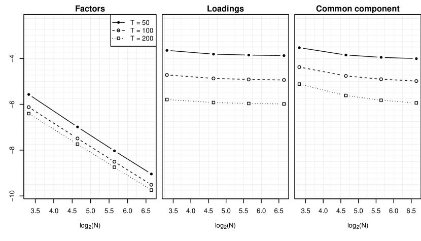
(b) Simulation scenario DGP2.

Figure 1: Estimations errors (in $\log_{2}$ scale) for DGP1 (subfigure (a)) and DGP2 (subfigure (b)). For each subfigure, we provide the estimation error for the factors ($\log_{2}\delta_{N,T}^{2}$, left), loadings ($\log_{2}{\varepsilon}_{N,T}^{2}$, middle), and common component ($\log_{2}\phi_{N,T}$, right, $\phi_{N,T}$ defined in (5.1)) as functions of $\log_{2}N$. The scales on the vertical axes are the same. Each curve corresponds to one value of $T\in\{50,100,200\}$, sampled for $N\in\{10,25,50,100\}$.

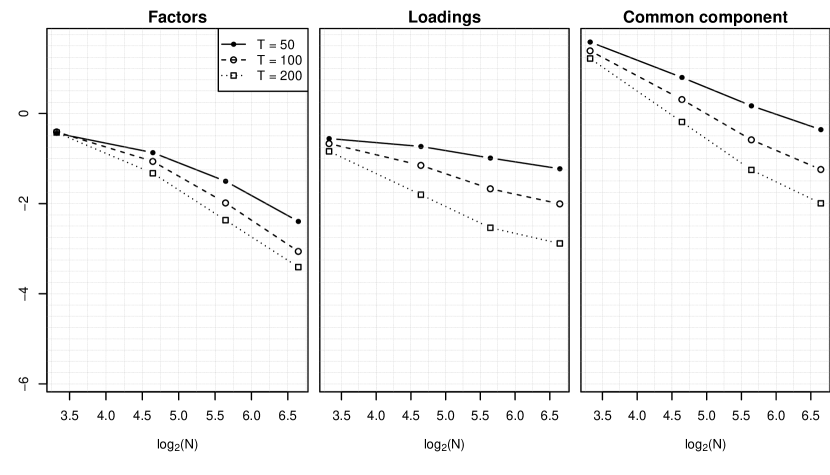
(a) Simulation scenario DGP3.

(b) Simulation scenario DGP4.

Figure 2: Estimations errors (in $\log_{2}$ scale) for DGP3 (subfigure (a)) and DGP4 (subfigure (b)). For each subfigure, we have the estimation error for the factors ($\log_{2}\delta_{N,T}^{2}$, left), loadings ($\log_{2}{\varepsilon}_{N,T}^{2}$, middle), and common component ($\log_{2}\phi_{N,T}$, right, $\phi_{N,T}$ defined in (5.1)) as functions of $\log_{2}N$. The scales of the vertical axes are the same. Each curve corresponds to one value of $T\in\{50,100,200\}$, sampled for $N\in\{10,25,50,100\}$.

Results for DGP3 and DGP4 are shown in Figure 2. A comparison between DGP3, DGP4 and DGP1, DGP2 is interesting because they only differ by the scale of the idiosyncratic components. We see that the errors are much higher for DGP3, DGP4 than for DGP1, DGP2, as expected. Notice that the dominant term for the factors is no longer of order $N^{-1}$ over all values of $N,T$: it seems to kick in for $N\in[25,100]$ in DGP3, DGP4, but looks slightly higher than $N^{-1}$ for $N\in[10,25]$ and $T\in[100,200]$ in DGP4 (noticeably so for $T=200$). A similar phenomenon occurs for the loadings and common component in DGP4, for $N\in[10,25]$ and $T=200$. These rates do not contradict the theoretical results of Section 4.2, which hold for $N,T\to\infty$, so DGP4, in particular, indicates that the values of $N$ considered there are too small for the asymptotics to have kicked in, and prompts further theoretical investigations about the estimation error rates in finite samples.

5.2 Estimation of the number of factors

Following the results of Section 3.2, we suggest a data-driven identification of the number $r$ of factors. Recall the definition of ${\cal X}_{N,T}$ in (2.1). The criteria that we will use for identifying the number of factors are combining the information-theoretic criteria described in Section 3.2 with the tuning and permutation-enhanced method of Alessi et al. (2009b) (ABC below). That method considers criteria of the form

(5.2) $$\mathrm{IC}(c,{\cal X}_{N,T},k)\vcentcolon=V(k,\widetilde{{\bm{U}}}^{(k)}_{T})+c\,k\,g(N,T),$$

which is the same as (3.3), but with a tuning $c>0$ of the penalty term. Indeed, if a penalty function $g(N,T)$ satisfies the assumptions of Theorem 4.1, then $c\,g(N,T)$ also satisfies these assumptions. The choice of the tuning parameter $c$ itself is data-driven, which allows the information criterion to be calibrated for each dataset.

In the ABC methodology, one estimates $r$ for a grid $C=\{c_{i}:\;i=1,\ldots,I\}$ of tuning parameter values. For every point in the grid, we shuffle the cross-sectional order several times then create sub-panels of sizes $\{(N_{j},T_{j}),\,j=1,\ldots,J\}$ with $(N_{J},T_{J})=(N,T)$ by selecting the top-left part of the panel. For every $i$ and $j$, we repeat these procedures $P$ times on random permutations of the cross-sectional order. For every $i=1,\ldots,I$, $j=1,\ldots,J$, and every permutation $p=1,\ldots,P$, we compute

(5.3) $$\hat{r}(c_{i},j,p)\vcentcolon=\operatorname*{arg\,min}_{k=1,\ldots,k_{\mathrm{max}}}\mathrm{IC}(c_{i},{\cal X}_{N_{j},T_{j}}^{(p)},k).$$

Define now the sample $\hat{r}_{i,p}\vcentcolon=\{\hat{r}(c_{i},j,p):j=1,\ldots,J\}$. One finally selects the optimal scaling $\hat{c}_{i,p}$ as the middle value of the second plateau of the function $c_{i}\rightarrow\mathrm{Var}\big{[}\hat{r}_{i,p}\big{]}$ and the number $\hat{r}$ of factors as the median of $\{\hat{r}(\hat{c}_{i,p},J,p):p=1,\ldots,P\}$. The consistency of $\hat{r}$ readily follows from that of the “un-tuned” method—see Hallin & Liška (2007) for details.

For our simulation, we have adopted $k_{\mathrm{max}}\vcentcolon=10$, $P\vcentcolon=5$, $N_{j}\vcentcolon=\left\lfloor\frac{4N}{5}+N(j-1)/45\right\rfloor$ $(j=1,\ldots,10)$, and $T_{j}\vcentcolon=T$, with a grid $C=\{0,0.05,0.1,\ldots,10\}$ for the values of $c$ and the following adaptations of the IC1 and IC2 penalty functions of Bai & Ng (2002):

$$g_{\texttt{IC1a}}(N,T) \vcentcolon=\sqrt{\frac{N+T}{NT}}\log\bigg{(}\frac{NT}{N+T}\bigg{)},$$

$$g_{\texttt{IC2a}}(N,T) \vcentcolon=\sqrt{\frac{N+T}{NT}}\log C_{N,T}^{2}.$$

In order to analyze the performance of the corresponding identification procedures, we have generated data based on DGP1 for $N\in\{10,25,50,100\}$ and $T\in\{25,50,100,200\}$. Among 100 replications, we have counted the number of overestimations and underestimations of $r$. The results are displayed in Table 1. We see that the number of factors is almost perfectly estimated if $N\geq 50$ or $T\geq 100$, or if $N\geq 25$ and $T\geq 50$. Furthermore, that number is almost never overestimated. For smaller panel sizes ($N=10,T=25$—but this is really very small) the criteria give a correct estimate about half of the time, with the other half yielding an underestimation.

	IC1a				IC2a
	$T\!=\!25$	$T\!=\!50$	$T\!=\!100$	$T\!=\!200$	$T\!=\!25$	$T\!=\!50$	$T\!=\!100$	$T\!=\!200$
$N=10$	52 (0)	17 (0)	1 (0)	0 (0)	54 (0)	20 (0)	1 (0)	0 (0)
$N=25$	13 (0)	0 (0)	0 (0)	0 (0)	15 (0)	0 (0)	0 (0)	0 (0)
$N=50$	2 (1)	0 (0)	0 (0)	0 (0)	2 (0)	0 (0)	0 (0)	0 (0)
$N=100$	0 (1)	0 (0)	0 (0)	0 (0)	0 (1)	0 (0)	0 (0)	1 (0)

Table 1: Number of underestimation (overestimation) of the number of factors using IC1a, IC2a among 100 replications of DGP1.

5.3 Estimation with Misspecified Number of Factors

The influence on the estimation of the common component of a misspecification of the number of factors is investigated in Section F.1 of the Appendices. The estimation error appears to be smallest when the estimated number of factor is correctly identified, provided that $N$ and $T$ are “large enough,” where “large enough” depends on the ratio between total idiosyncratic and total common variances; see Section F.1 in the Appendices for a detailed discussion.

6 Forecasting of mortality curves

In this section, we show how the theory developed can be used to accurately forecast a high-dimensional vector of FTS. We consider the National Institute of Population and Social Security Research (2020) dataset that contains age-specific and gender-specific mortality rates for the 47 Japanese prefectures from 1975 through 2016. For every prefecture and every year, the mortality rates are grouped by gender (Male or Female) and by age (from 0 to 109). People aged 110+ are grouped together in a single rate value. Gao et al. (2018) used this specific dataset to show that their method outperforms existing FTS methods. We will use the same dataset to show that our method in turn outperforms Gao et al. (2018).

Due to sparse observations at old ages, we have grouped the observations related to the age groups of 95 or more by averaging the mortality rates and denote by $x_{it}(\tau)$, $i=1,\ldots,47$; $t=1,\ldots,42$; $\tau=0,1,\ldots,95$ the log mortality rate of people aged $\tau$ living in prefecture $i$ during year $1974+t$. The dataset contains many missing values which we replaced with the rates of the previous age group. We conducted separate analyses for males and females, making our forecasting results comparable to those in Gao et al. (2018).

The three $h$-step ahead forecasting methods to be compared are

1. The method of Gao et al. (2018), implemented via the dedicated functions of their R package ftsa (Shang, 2013), with the smoothing technique and the parameter values they suggested for this dataset.

2. Componentwise forecasting. For each of the $N$ functional time series in the panel, we fitted a functional model independently of the other functional time series. As it is common in functional time series, we obtain the forecast by decomposing every function on its principal components, forecasting every functional principal component score separately and recomposing the functional forecast based on the score forecasts (cf. for instance Hyndman & Ullah, 2007; Hyndman & Shang, 2009). For this exercise, we have used six functional principal components and ARMA models to predict the scores.

3. Our $h$-step ahead forecasting method, which we now describe.

The smoothing technique we have used differs from the one considered by Gao et al. (2018) since the latter results in a 96-points representation of the curves while our method is computationally more efficient with data represented in a functional basis. Thus, in order to implement our method, we transform the regularly-spaced data points into curves represented on a 9-dimensional B-splines basis. In our notation, $H_{i}\vcentcolon=L^{2}([0,\,95],\mathbb{R})$, $i=1,\ldots,47$. Our $h$-step ahead forecasting algorithm, based on the data $\{x_{it}:i=1,\ldots,47;\,t=1,\ldots,T\}$ with $T\leq 42$, works as follows.

1. Compute $\hat{r}$ using the permutation-enhanced ABC methodology with the same parameters as in Section 5.2 and the IC2a penalization function.

2. For $i=1,\ldots,N$, compute the $i$th sample mean $\hat{\mu}_{i}\vcentcolon=\sum_{t=1}^{T}x_{it}/T$ and the centered panel $y_{it}\vcentcolon=x_{it}-\hat{\mu}_{i}$.

3. Compute the estimated factors $\{\tilde{{\bm{u}}}^{(\hat{r})}_{t}:t=1,\ldots,T\}$ and factor loadings $\widetilde{{\bm{B}}}^{(\hat{r})}_{N}$ using Proposition 3.1, and compute the common component $\hat{\chi}_{it}^{(\hat{r})}$ using (3.2); compute the estimators $\hat{\xi}^{(\hat{r})}_{it}\vcentcolon=y_{it}-\hat{\chi}_{it}^{(\hat{r})}$, $i=1,\ldots,N$ and $t=1,\ldots,T$ of the idiosyncratic components.

4. For each $l\in\{1,\ldots,\hat{r}\}$, select the ARIMA model that best models the $l$-thfactor $\{u_{l,t}^{(\hat{r})}:t=1,\ldots,T\}$ according to the BIC criterion; forecast $\tilde{{\bm{u}}}^{(\hat{r})}_{T+h}$ based on these fitted models, using past values $\{u_{l,t}^{(\hat{r})}:t=1,\ldots,T\}$.

5. For every $i\in\{1,\ldots,N\}$, pick the ARIMA model that best models the idiosyncratic component $\{\hat{\xi}^{(\hat{r})}_{it}:t=1,\ldots,T\}$ according to the BIC criterion, and forecast $\hat{\xi}^{(\hat{r})}_{i,T+h}$ based on the fitted model, using past values $\hat{\xi}^{(\hat{r})}_{it}$ up to $t=T$.

6. The final forecast is $\hat{x}_{i,T+h}\vcentcolon=\hat{\mu}_{i}+\tilde{b}^{(\hat{r})}_{i}\tilde{{\bm{u}}}^{(\hat{r})}_{T+h}+\hat{\xi}^{(\hat{r})}_{i,T+h},$ where $\tilde{b}^{(\hat{r})}_{i}\vcentcolon=\mathsf{P}_{i}\widetilde{{\bm{B}}}^{(\hat{r})}_{N}$, and $\mathsf{P}_{i}:{\bm{H}}_{N}\to H_{i}$ maps $(v_{1},\ldots,v_{N})^{\mathsf{T}}\in{\bm{H}}_{N}$ to $v_{i}\in H_{i}$.

In order to properly assess the forecasting accuracy of each method, we split the dataset into a training set and a test set. The training set consists of the observations from 1975 to $1974+\Delta$, which translates into $t=1,\ldots,\Delta$. The test set consists of the observations for the years $1974+\Delta+1$ and subsequent ($t\geq\Delta+1$). For every rolling window $t=1,\ldots,\Delta$, we re-estimate the parameters of our model and those from Gao et al. (2018).

To ensure that our forecasts imply positive mortality rates, we have applied the log transform to the mortality curves. Log transforms are quite classical in that area of statistical demography (cf. Hyndman & Ullah, 2007; Hyndman & Shang, 2009; He et al., 2021). Gao et al. (2018) have also used the log curves for estimating their model but, in the last stage of their forecasting analysis, they compute the exponentials of their forecasted log curves and base their metrics on it. However, the female mortality rate for $95$+ is $1645$ times larger than the mortality rate for age $10$ and $345$ times larger than the mortality rate at age 40 (averaged across time and the Japanese regions). Similar results hold for male mortality curves. This fact just illustrates that the scale of the mortality rates differs greatly from one age to another. Hence, in the analysis of Gao et al. (2018), the contribution of the young ages to the averaged errors is negligible. Assessing the quality of a model’s predictions based on a metric that disregards most of the predictions may be misleading. In accordance with the demographic practice, we thus decided to establish our comparisons on a metric based on the log curves. For the sake of completeness, we also present the results based on the methodology of Gao et al. (2018) in Section G of the Appendices.

Comparisons are conducted using the mean absolute forecasting error (MAFE) defined as

$${\text{MAFE}}(h)\vcentcolon=\frac{1}{47\times 89\times(17-h)}\sum_{i=1}^{47}\sum_{\Delta=26}^{42-h}\sum_{\tau=0}^{89}\Big{|}{\hat{x}_{i,\Delta+h}(\tau/89)-x_{i,\Delta+h}(\tau/89)}\Big{|},$$

and the mean squared forecasting error (MSFE) defined as

$${\text{MSFE}}(h)\vcentcolon=\frac{1}{47\times 89\times(17-h)}\sum_{i=1}^{47}\sum_{\Delta=26}^{42-h}\sum_{\tau=0}^{89}\Big{[}\hat{x}_{i,\Delta+h}(\tau/89)-x_{i,\Delta+h}(\tau/89)\Big{]}^{2}.$$

Notice that $\Delta=26$ corresponds to the year $2000$, and that $\Delta=42-h$ corresponds to the year $2016-h$. These forecasting errors are given in Table 2. The results indicate that our method markedly outperforms the other methods for all $h$, for both measures of performance (MAFE and MSFE), an for both the male and female panels. This is not surprising, since our method does not lose cross-sectional information by separately estimating factor models for the various principal components of the cross-section as the GSY method does; nor does it ignore the interrelations between the $N$ functional time series as CF does.

	Female						Male
	MAFE			MSFE			MAFE			MSFE
	GSY	CF	TNH	GSY	CF	TNH	GSY	CF	TNH	GSY	CF	TNH
$h=1$	296	286	250	190	166	143	268	232	221	167	124	122
$h=2$	295	294	252	187	171	145	271	243	224	171	131	124
$h=3$	294	301	254	190	176	148	270	252	227	170	136	126
$h=4$	300	305	258	195	178	152	274	259	230	177	141	129
$h=5$	295	308	259	190	179	154	270	268	233	169	146	131
$h=6$	295	313	259	194	181	156	271	278	235	169	152	134
$h=7$	302	321	263	200	187	161	266	289	240	164	160	138
$h=8$	298	329	269	192	193	167	266	302	245	161	168	142
$h=9$	303	339	275	203	199	172	277	315	251	169	178	148
$h=10$	308	347	280	209	205	177	283	327	254	174	186	150
Mean	299	314	262	195	183	157	272	277	236	169	152	134
Median	297	311	259	193	180	155	271	273	234	169	149	133

Table 2: Comparison of the forecasting accuracies of our method (denoted as TNH ) with Gao et al. (2018) (denoted as GSY) and with componentwise FTS forecasting (denoted CF) on the Japanese mortality curves for $h=1,\ldots,10$, female and male curves. Boldface is used for the winning MAFE and MSFE values, which uniformly correspond to the TNH forecast. Both metrics have been multiplied by $1000$ for readability.

7 Discussion

This paper proposes a new paradigm for the analysis of high-dimensional time series with functional (and possibly also scalar) components. The approach is based on a new concept of (high-dimensional) functional factor model which, in the particular case of purely scalar series reduces to the the well-established concepts studied by Stock & Watson (2002a, b) and Bai & Ng (2002), albeit under weaker assumptions. We extend to the functional context the classical representation results of Chamberlain (1983); Chamberlain & Rothschild (1983) and propose consistent estimation procedures for the common components, the factors, and the factor loadings as both the size $N$ of the cross-section and the length $T$ of the observation period tend to infinity, with no constraints on their relative rates of divergence. We also propose a consistent identification method for the number of factors, extending to the functional context the methods of Bai & Ng (2002) and Alessi et al. (2010).

This is, however, only a first step in the development of a full-fledged toolkit for the analysis of high-dimensional time series, and a long list of important issues remains on the agenda of future research. This includes, but is not limited to, the following points.

1. This paper only considers consistency of the estimates. Further asymptotic analysis should be developed in the direction of consistency rates and asymptotic distributions, on the model of Bai (2003); Forni et al. (2004); Lam & Yao (2012) or Forni et al. (2017).

2. The factor model developed here is an extension of the static scalar models by Stock & Watson (2002a, b) and Bai & Ng (2002), where factor loadings are matrices. That factor model is only a particular case of the general (also called generalized) dynamic factor model introduced by Forni et al. (2000), where factors are loaded in a fully dynamic way via filters (see Hallin & Lippi (2013) for the advantages that generalized approach). An extension of the general dynamic factor model to the functional setting is, of course, highly desirable, but requires a more general representation result involving filters with operatorial coefficients and the concept of functional dynamic principal components (Panaretos & Tavakoli, 2013a; Hörmann et al., 2015).

3. The problem of identifying the number of factors is only briefly considered here, and requires further attention. In particular, functional versions of the eigenvalue-based methods by Onatski (2009, 2010) or the hypothesis testing-based ones by Pan & Yao (2008); Kapetanios (2010); Lam & Yao (2012); Ahn & Horenstein (2013) deserve being developed and compared to the method we are proposing here.

4. Another crucial issue is the analysis of volatilities. In the scalar case, the challenge is in the estimation and forecasting of high-dimensional conditional covariance matrices and such quantities as values-at-risk or expected shortfalls: see Fan et al. (2008, 2011, 2013); Barigozzi & Hallin (2016, 2017); Trucios et al. (2019). In the functional context, these matrices, moreover, are replaced with high-dimensional operators.

Acknowledgements

We would like to thank Yoav Zemel, Gilles Blanchard and Yuan Liao for helpful technical discussions, as well as Yuan Gao and Hanlin Shang for details of the implementation of the forecasting methods described in Gao et al. (2018). Finally, we thank the referees and the associate editor for comments leading to an improved version of the paper.

Code

The R code reproducing the numerical experiments of Section 5, as well as code used for Section 6, can be obtained by contacting the authors by email.

Appendix A Orthogonal Projections

Let $H$ be a separable Hilbert space. Denote by $L^{2}_{H}\left(\Omega\right)$ the space of $H$-valued random elements $X:\Omega\rightarrow H$ with $\operatorname{\>{\mathbb{E}}}\!X\!=0$ and $\operatorname{\>{\mathbb{E}}}\!{\left\lVert X\right\rVert}_{H}^{2}\!<\leavevmode\nobreak\ \!\infty$. For any finite-dimensional subspace $\mathcal{U}\subset L^{2}\!\left(\Omega\right)$, where $L^{2}\!\left(\Omega\right)$ is the set of random variables with mean zero and finite variance, let

(A.1) $$\operatorname{\mathrm{span}}_{H}(\mathcal{U})\vcentcolon=\left\{\sum_{j=1}^{m}u_{j}b_{j}:b_{j}\in H,\,u_{j}\in\mathcal{U},\,m=1,2,\ldots\right\}.$$

Since $\mathcal{U}$ is finite-dimensional, $\operatorname{\mathrm{span}}_{H}(\mathcal{U})\subseteq L^{2}_{H}\left(\Omega\right)$ is a closed subspace. Indeed, denoting by $u_{1},\ldots,u_{r}\in\leavevmode\nobreak\ \!{\mathcal{U}}$ ($r<\infty$) an orthonormal basis,

$$\operatorname{\>{\mathbb{E}}}{\left\lVert u_{1}b_{1}+\cdots+u_{r}b_{r}\right\rVert}_{H}^{2}={\left\lVert b_{1}\right\rVert}_{H}^{2}+\cdots+{\left\lVert b_{r}\right\rVert}_{H}^{2}.$$

By the orthogonal decomposition Theorem (Hsing & Eubank 2015, Theorem 2.5.2), for any $X\in L^{2}_{H}\left(\Omega\right)$, there exists a unique $U[X]\in\operatorname{\mathrm{span}}_{H}(\mathcal{U})$ such that

(A.2) $$X=U[X]+V[X],$$

where $V[X]=X-U[X]\in\operatorname{\mathrm{span}}_{H}(\mathcal{U})^{\perp}$; hence ${\mathbb{E}\left[uV[X]\right]}=0$ for all $u\in\mathcal{U}$ and

(A.3) $$\operatorname{\>{\mathbb{E}}}{\left\lVert X\right\rVert}_{H}^{2}=\operatorname{\>{\mathbb{E}}}{\left\lVert U[X]\right\rVert}_{H}^{2}+\operatorname{\>{\mathbb{E}}}{\left\lVert V[X]\right\rVert}_{H}^{2}.$$

Consider the following definition.

Definition A.1.

The decomposition (A.2) of $X\in L^{2}_{H}\left(\Omega\right)$ into $U[X]$ and $V[X]$ is called the orthogonal decomposition of $X$ onto $\operatorname{\mathrm{span}}_{H}(\mathcal{U})$ and its orthogonal complement; $U[X]=\vcentcolon\operatorname{\mathrm{proj}}_{H}(X|\mathcal{U})$ is the orthogonal projection of $X$ onto $\operatorname{\mathrm{span}}_{H}(\mathcal{U})$.

If $u_{1},\ldots,u_{r}\in L^{2}\!\left(\Omega\right)$ form a basis of $\mathcal{U}$, then $\operatorname{\mathrm{proj}}_{H}(X|\mathcal{U})=\sum_{l=1}^{r}u_{l}b_{l}$ for some unique $b_{1},\ldots,b_{r}\in H$; if they form an orthonormal basis, then $b_{l}={\mathbb{E}\left[u_{l}X\right]}$, $l=1,\ldots,r$. We shall also use the notation

$$\operatorname{\mathrm{proj}}_{H}(X|{\bm{u}})\vcentcolon=\operatorname{\mathrm{proj}}_{H}(X|u_{1},\ldots,u_{r})\vcentcolon=\operatorname{\mathrm{proj}}_{H}(X|\mathcal{U}),$$

and

$$\operatorname{\mathrm{span}}_{H}({\bm{u}})\vcentcolon=\operatorname{\mathrm{span}}_{H}(\mathcal{U}),$$

where $\mathcal{U}=\operatorname{\mathrm{span}}(u_{1},\ldots,u_{r})$ and ${\bm{u}}=(u_{1},\ldots,u_{r})^{\mathsf{T}}\in\mathbb{R}^{r}$. Notice that if ${\mathbb{E}\left[{\bm{u}}{\bm{u}}^{\mathsf{T}}\right]}=\bm{I}_{r}$ (with $\bm{I}_{r}$ the $r\times r$ identity matrix), then

(A.4) $$\operatorname{\mathrm{proj}}_{H}(X|{\bm{u}})={\mathbb{E}\left[X\operatorname*{\otimes}{\bm{u}}\right]}{\bm{u}}.$$

Appendix B Advantage of Proposed Approach

This section provides examples where the approach proposed by Gao et al. (2018), contrary to ours, runs into serious problems. In Gao et al. (2018), each series $\{x_{it}:t\in\mathbb{Z}\}$ is first projected onto the first $p_{0}$ eigenfunctions of the long-run covariance operator,

$$C^{(x_{i})}\vcentcolon=\sum_{t\in\mathbb{Z}}{\mathbb{E}\left[x_{it}\operatorname*{\otimes}x_{i0}\right]}.$$

Consider the high-dimensional functional factor model with $r\in\mathbb{N}$ factors

$$x_{it}=b_{i1}u_{1t}+\cdots+b_{ir}u_{rt}+\xi_{it},\quad i=1,2,\ldots,\ t\in\mathbb{Z},$$

where $b_{i1},\ldots,b_{ir}\in H_{i}$ are deterministic, $i\geq 1$. If we assume that ${\mathbb{E}\left[{\bm{u}}_{t}\operatorname*{\otimes}{\bm{\xi}}_{s}\right]}={\bf 0}$ for all $s,t\in\mathbb{Z}$, the long-run covariance operator of $\{x_{it}:t\in\mathbb{Z}\}$ is

$$C^{(x_{i})}=\sum_{t\in\mathbb{Z}}{\mathbb{E}\left[x_{it}\operatorname*{\otimes}x_{i0}\right]} =\sum_{t\in\mathbb{Z}}\left({\mathbb{E}\left[(\bm{b}_{i}{\bm{u}}_{t})\operatorname*{\otimes}(\bm{b}_{i}{\bm{u}}_{0})\right]}+{\mathbb{E}\left[\xi_{it}\operatorname*{\otimes}\xi_{i0}\right]}\right)$$

$$=\bm{b}_{i}C^{(u)}\bm{b}_{i}^{\star}+C^{(\xi_{i})},$$

where $\bm{b}_{i}\in\mathcal{L}(\mathbb{R}^{r},H_{i})$ maps $(u_{1},\ldots,u_{r})^{\mathsf{T}}\in\mathbb{R}^{r}$ to $u_{1}b_{i1}+\cdots+u_{r}b_{ir}\in H_{i}$,

$${\bf C}^{(u)}\vcentcolon=\sum_{t\in\mathbb{Z}}{\mathbb{E}\left[{\bm{u}}_{t}\operatorname*{\otimes}{\bm{u}}_{0}\right]},\quad\text{ and}\quad C^{(\xi_{i})}\vcentcolon=\sum_{t\in\mathbb{Z}}{\mathbb{E}\left[\xi_{it}\operatorname*{\otimes}\xi_{i0}\right]}.$$

Let

$${\bf C}^{(u)}=\sum_{j=1}^{r}\lambda_{j}^{(u)}{\bf v}_{j}^{(u)}\operatorname*{\otimes}{\bf v}_{j}^{(u)}\quad\text{and}\quad C^{(\xi_{i})}=\sum_{j=1}^{\infty}\lambda_{j}^{(\xi_{i})}{\varphi}_{j}^{(\xi_{i})}\operatorname*{\otimes}{\varphi}_{j}^{(\xi_{i})}$$

denote the eigen-decompositions of ${\bf C}^{(u)}$ and $C^{(\xi_{i})}$, respectively. Then,

(B.1) $$C^{(x_{i})}=\sum_{j=1}^{r}\lambda_{j}^{(u)}{\bf v}_{j}^{(u)}\operatorname*{\otimes}{\bf v}_{j}^{(u)}+\sum_{j=1}^{\infty}\lambda_{j}^{(\xi_{i})}{\varphi}_{j}^{(\xi_{i})}\operatorname*{\otimes}{\varphi}_{j}^{(\xi_{i})}.$$

If ${\varphi}_{j}^{(\xi_{i})}$ is orthogonal to $b_{i1},\ldots,b_{ir}\in H_{i}$, $j\geq 1$, we can choose $\lambda_{j}^{(\xi_{i})},j=1,\ldots,J$, large enough that

1. the first $J$ eigenvectors of $C^{(x_{i})}$ are ${\varphi}_{j}^{(\xi_{i})}$, with associated eigenvalues $\lambda_{j}^{(\xi_{i})}$, $j=1,\ldots J$;

2. the proportion $\sum_{j=1}^{J}\lambda_{j}^{(\xi_{i})}/\operatorname{{\mathrm{Tr}}}(C^{(x_{i})})$ of variance explained by the first $J$ principal components of $\{x_{it}:t\in\mathbb{Z}\}$ is arbitrarily close to $1$.

In such a case, the preliminary FPCA approximation of each series $\{x_{it}:t\in\mathbb{Z}\}$ in Gao et al. (2018) (at population level, based on the true long-run covariance of $C^{(x_{i})}$) would completely discard the common component. Since we do not perform such preliminary FPCA approximation, the common component would not get lost with our method (see results for DGP4, Figure 2(b), for the empirical performance of our method in a similar situation). A similar point can be made if one performs, as a preliminary step, the usual FPCA projection of each series based on the lag-$0$ covariance operators ${\mathbb{E}\left[x_{i0}\operatorname*{\otimes}x_{i0}\right]}$ (as opposed to the long-run covariance), or even a more sophisticated dynamic FPCA projection (Panaretos & Tavakoli 2013a, Hörmann et al. 2015).

Appendix C Uniform error bounds on loadings and the common component

In this Section, we provide uniform error bounds for the loadings and the common component. All the results in this Section are proved in Section D.7.

We first turn our attention to the loadings. Let ${\bm{b}}_{i}\in\mathcal{L}(\mathbb{R}^{r},H_{i})$ be the linear operator mapping $(\alpha_{1},\ldots,\alpha_{r})^{\mathsf{T}}$ to $\sum_{l=1}^{r}\alpha_{l}b_{il}$. The estimator of ${\bm{b}}_{i}$ is $\tilde{{\bm{b}}}^{(r)}_{i}\!=\mathsf{P}_{i}\widetilde{{\bm{B}}}^{(r)}\!$, where $\mathsf{P}_{i}:\leavevmode\nobreak\ \!{\bm{H}}_{N}\to\leavevmode\nobreak\ \!H_{i}$ is the canonical projection, mapping $(v_{1},\ldots,v_{N})^{\mathsf{T}}\in{\bm{H}}_{N}$ to $v_{i}\in H_{i}$, $i=1,\ldots,N$. With this notation, notice that ${\bm{b}}_{i}=\mathsf{P}_{i}{\bm{B}}_{N}$. To get uniform error bounds for the loadings, we need some technical assumptions, which rely on the concept of $\tau$-mixing: for a sequence of random elements $\{Y_{t}\}\subset H_{0}$ such that ${\left\lVert Y_{t}\right\rVert}_{H_{0}}\leq c$ almost surely, where $H_{0}$ is a real separable Hilbert space with norm ${\left\lVert\cdot\right\rVert}_{H_{0}}$, we define the $\tau$-mixing coefficients (Blanchard & Zadorozhnyi 2019, Example 2.3)

(C.1) $$\tau(h)\vcentcolon=\sup\Big{\{}{\mathbb{E}\left[Z({\varphi}(Y_{t+h})-\operatorname{\>{\mathbb{E}}}{\varphi}(Y_{t+h}))\right]}\leavevmode\nobreak\ \Big{|}\leavevmode\nobreak\ t\geq 1,Z\in L^{1}(\Omega,\mathcal{M}^{Y}_{t},\operatorname{{\mathbb{P}}}),$$

$$\hskip 142.26378pt\operatorname{\>{\mathbb{E}}}{\left|Z\right|}\leq 1,{\varphi}\in\mathsf{\Lambda}_{1}(H_{0},c)\Big{\}},$$

where $\mathcal{M}^{Y}_{t}$ is the $\sigma$-algebra generated by $Y_{1},\ldots,Y_{t}$ and, denoting by $B_{c}(H_{0})\subset H_{0}$ the ball of radius $c>0$ centered at zero,

$$\mathsf{\Lambda}_{1}(H_{0},c)\vcentcolon=\Big{\{}{\varphi}:B_{c}(H_{0})\to\mathbb{R}\text{ such that }{\left|{\varphi}(x)-{\varphi}(y)\right|}\leq{\left\lVert x-y\right\rVert}_{H_{0}},\forall x,y\in H_{0}\Big{\}}.$$

Notice that by the Kirszbraun Theorem (Schwartz 1965, Theorem 1.31), the definition of $\tau(h)$ is independent of the choice of upper bound $c>0$.

For obtaining uniform bounds on the loadings, we make the following assumptions.

Assumption H($\gamma$).

(H1)

For all $l=\leavevmode\nobreak\ \!1,\ldots,r$ and all $i,t\geq 1$, ${\mathbb{E}\left[u_{lt}\xi_{it}\right]}=0,$

$$\left\lvert u_{lt}\right\rvert<c_{u}<\infty\quad\text{and}\quad{\left\lVert\xi_{it}\right\rVert}_{H_{i}}\leq c_{\xi}<\infty\quad\text{almost surely. }$$

(H2)

There exists $\alpha,\theta,\gamma>0$ such that, for all $l=1,\ldots,r$ and all $i\geq\leavevmode\nobreak\ \!1$, the process

$$\{(u_{lt},\xi_{it}):t=1,2,\ldots\}\subset\mathbb{R}\oplus H_{i}$$

is $\tau$-mixing with coefficient $\tau(h)\leq\leavevmode\nobreak\ \!\alpha\exp(-(\theta h)^{\gamma})$.

Assumption H($\gamma$) is needed in order to apply Bernstein-type concentration inequalities for $T^{-1}\sum_{s=1}^{T}u_{ls}\xi_{is}$ (Blanchard & Zadorozhnyi 2019), and could be replaced by any other technical condition that yields such concentration bounds. Notice that we do not assume joint $\tau$-mixing on the cross-section of idiosyncratics and factors. Assumption (H2) is implied by the stronger (joint $\tau$-mixing) assumption that

$$\Big{\{}(u_{1t},\ldots,u_{rt},\xi_{1t},\xi_{2t},\ldots):t\geq 1\Big{\}}\subset\mathbb{R}^{r}\oplus\bigoplus_{i\geq 1}H_{i}$$

is exponentially $\tau$-mixing. Such a joint assumption on all factors and idiosyncratics is made in Fan et al. (2013), but with $\alpha$-mixing instead of $\tau$-mixing. Note that $\alpha$-mixing coefficients are not comparable to $\tau$-mixing coefficients. However, $\tau$-mixing holds for some simple AR$(1)$ models that are not $\alpha$-mixing. Examples of $\tau$-mixing processes can be found in Blanchard & Zadorozhnyi (2019). Other types of mixing coefficients equivalent to $\tau$-mixing when the random elements are almost surely bounded are the $\theta_{\infty}$-mixing coefficients (Dedecker et al. 2007, Definition 2.3) or the $\tau_{\infty}$-mixing coefficients (Olivier 2010, p.492).

We can now state a uniform error bound result for the estimators of ${\bm{b}}_{i},i=1,\ldots,N$.

Theorem C.1.

Let Assumptions A, B, C, D and H($\gamma$) hold. Then,

$$\max_{i=1,\ldots,N}{\left|\kern-0.86108pt\left|\kern-0.86108pt\left|\tilde{{\bm{b}}}^{(r)}_{i}-{\bm{b}}_{i}\tilde{\bm{R}}^{-1}\right|\kern-0.86108pt\right|\kern-0.86108pt\right|}_{2}=O_{\rm P}\left(\max\left\{\frac{1}{\sqrt{N}},\frac{\log(N)\log(T)^{1/{2\gamma}}}{\sqrt{T}}\right\}\right).$$

We see that if $N,T\to\infty$ with $\log(N)=o(\sqrt{T}/\log(T)^{1/{2\gamma}})$, the estimator of the loadings is uniformly consistent. We notice that in the special case ${\bm{H}}_{N}=\mathbb{R}^{N}$, Fan et al. (2013) do not impose boundedness assumptions on the factors and idiosyncratics, but rather impose exponential tail bounds on them. They impose exponential $\alpha$-mixing conditions on the factors and idiosyncratics (jointly), whereas we impose exponential $\tau$-mixing on the product of factors and idiosyncratics. Their rate of convergence is similar, except for the $\log(N)\log(T)^{1/{2\gamma}}$ factor, which appears as $\sqrt{\log(N)}$ in their case. The reason for our different rates of convergence is that we rely on concentration inequalities for weakly dependent time series in Hilbert spaces (Blanchard & Zadorozhnyi 2019), which are weaker and require stronger assumptions than their scalar counterparts (Merlevède et al. 2011). Having said that, whether these rates are optimal or whether the assumptions here are the weakest possible ones remain open questions.

The next result gives uniform bounds for the estimation of the common component. Recall the definition of $\hat{\chi}_{it}^{(r)}$ in (3.2).

Theorem C.2.

Under the assumptions of Theorems 4.8 and C.1,

$$\max_{t=1,\ldots T}\max_{i=1,\ldots,N}{\left\lVert\hat{\chi}^{(r)}_{it}-\chi_{it}\right\rVert}_{H_{i}}=O_{\rm P}\Big{(}\max\Big{\{}\frac{T^{1/(2\kappa)}}{\sqrt{N}},\frac{\log(N)\log(T)^{1/{2\gamma}}}{\sqrt{N}\,T^{(\kappa-1)/(2\kappa)}},$$

$$\hskip 199.16928pt\frac{\log(N)\log(T)^{1/{2\gamma}}}{\sqrt{T}}\Big{\}}\Big{)}.$$

If $N,T\to\infty$ with $T=o(N^{\kappa})$ and $\log(N)=o(\sqrt{T}/\log(T)^{1/{2\gamma}})$, the estimator of the common component is uniformly consistent, and the rate simplifies to

$$O_{\rm P}(\max\{T^{1/(2\kappa)}N^{-1/2},\ \log(N)\log(T)^{1/{2\gamma}}T^{-1/2}\}),$$

which yields some similarities to the rate in Fan et al. (2013, Corollary 1), though slightly different from it due to differences between our regularity assumptions.

Appendix D Proofs

Let $v_{i}\in H_{i}$: we write, with a slight abuse of notation, $v_{i}\in\leavevmode\nobreak\ \!\mathcal{L}(\mathbb{R},H_{i})$ for the mapping $v_{i}:\alpha\mapsto v_{i}\alpha\vcentcolon=\alpha v_{i}$ from $\mathbb{R}$ to $H_{i}$. Applying this notation for an ele- ment $\bm{v}=(v_{1},\ldots,v_{N})^{\mathsf{T}}$ of ${\bm{H}}_{N}$, we have that $\bm{v}\in\mathcal{L}(\mathbb{R},{\bm{H}}_{N})$ is the mapping $a\mapsto a\bm{v}$ from $\mathbb{R}$ to ${\bm{H}}_{N}$; in particular, ${\bm{v}}a=(av_{1},\ldots,av_{N})^{\mathsf{T}}$. Finally, let ${\left|\cdot\right|}$ denote the Euclidean norm in $\mathbb{R}^{p},p\geq 1$.

D.1 Proofs of Theorems 2.2 and 2.3

All proofs in this section are for some arbitrary but fixed $t$, with $N\rightarrow\infty$. Whenever possible, we therefore omit the index $t$, and write $\bm{X}_{N}$ for ${\bm{X}}_{N,t}\vcentcolon=(X_{1t},\ldots,X_{Nt})^{\mathsf{T}}$, etc. Denote by $\bm{\Sigma}_{N}={\mathbb{E}\left[{\bm{X}}_{N}\operatorname*{\otimes}{\bm{X}}_{N}\right]}$ the covariance operator of ${\bm{X}}_{N}$ which, in view of stationarity, does not depend on $t$. Denoting by $\bm{p}_{N,i}\in\leavevmode\nobreak\ \!{\bm{H}}_{N}$ the $i$th eigenvector of $\bm{\Sigma}_{N}$ and by $\lambda_{N,i}$ the corresponding eigenvalue, we have the eigendecomposition

$$\bm{\Sigma}_{N}=\sum_{i=1}^{\infty}\lambda_{N,i}\bm{p}_{N,i}\operatorname*{\otimes}\bm{p}_{N,i}.$$

The eigenvectors $\{\bm{p}_{N,i}:i\geq 1\}\subset{\bm{H}}_{N}$ form an orthonormal basis of theimage $\mathrm{Im}(\bm{\Sigma}_{N})\subseteq\leavevmode\nobreak\ {\bm{H}}_{N}$ of $\bm{\Sigma}_{N}$. We can extend this set of eigenvectors of $\bm{\Sigma}_{N}$ to form an orthonormal basis of ${\bm{H}}_{N}$. With a slight abuse of notation, we shall denote this basis by $\{\bm{p}_{N,i}:i\geq 1\}$, possibly reordering the eigenvalues: we might no longer have non-increasing and positive eigenvalues, but still can enforce $\lambda_{N,1}\geq\cdots\geq\lambda_{N,r+1}\geq\lambda_{N,r+1+j}$ for all $j\geq 1$. Define

$$\bm{P}_{N}=\sum_{k=1}^{r}{\bm{p}}_{N,k}\operatorname*{\otimes}{\bm{z}}_{k}\in\mathcal{L}(\mathbb{R}^{r},{\bm{H}}_{N}),$$

where ${\bm{z}}_{k}$ is the $k$-th vector in the canonical basis of $\mathbb{R}^{r}$. Let

$$\ell_{2}\vcentcolon=\left\{\bm{\alpha}=(\alpha_{1},\alpha_{2},\ldots):\alpha_{i}\in\mathbb{R},\sum_{i}\alpha_{i}^{2}<+\infty\right\},$$

and let $\bm{\alpha}_{k}\in\ell_{2}$ be the $k$-th canonical basis vector, with $(\bm{\alpha}_{k})_{k}=1$ and $(\bm{\alpha}_{k})_{i}=0$ for $i\neq k$. Define

$$\bm{Q}_{N}\vcentcolon=\sum_{k=1}^{\infty}{\bm{p}}_{N,r+k}\operatorname*{\otimes}\bm{\alpha}_{k}\in\mathcal{L}(\ell_{2},{\bm{H}}_{N}).$$

Denote by $\bm{\Lambda}_{N}\in\mathcal{L}(\mathbb{R}^{r})$ the diagonal matrix with diagonal elements $\lambda_{N,1},\ldots,\lambda_{N,r}$, that is,

$$\bm{\Lambda}_{N}\vcentcolon=\sum_{k=1}^{r}\lambda_{N,k}{\bm{z}}_{k}\operatorname*{\otimes}{\bm{z}}_{k},$$

and define $\bm{\Phi}_{N}\in\mathcal{L}(\ell_{2})$ as

$$\bm{\Phi}_{N}\vcentcolon=\sum_{k=1}^{\infty}\lambda_{N,r+k}\bm{\alpha}_{k}\operatorname*{\otimes}\bm{\alpha}_{k}.$$

With this notation, we have

(D.1) $$\bm{\Sigma}_{N}=\bm{P}_{N}\bm{\Lambda}_{N}\bm{P}_{N}^{\star}+\bm{Q}_{N}\bm{\Phi}_{N}\bm{Q}_{N}^{\star}\in\mathcal{L}({\bm{H}}_{N})\quad\text{and}\quad\bm{P}_{N}\bm{P}_{N}^{\star}+\bm{Q}_{N}\bm{Q}_{N}^{\star}=\mathrm{Id}_{N},$$

where $\mathrm{Id}_{N}$ is the identity operator on ${\bm{H}}_{N}$. Let

(D.2) $$\bm{\psi}_{N}\vcentcolon=\bm{\Lambda}_{N}^{-1/2}\bm{P}_{N}^{\star}\bm{X}_{N}=(\lambda_{N,1}^{-1/2}\left\langle\bm{p}_{N,1},\bm{X}_{N}\right\rangle,\ldots,\lambda_{N,r}^{-1/2}\left\langle\bm{p}_{N,r},\bm{X}_{N}\right\rangle)^{\mathsf{T}}\in\mathbb{R}^{r}$$

(note that, by Lemma D.28, $\bm{\psi}_{N}$ is well defined for $N$ large enough since $\lambda_{N,r}\to\infty$ as ${N\to\infty}$). Using (D.1), we get

(D.3) $$\bm{X}_{N}=\bm{P}_{N}\bm{P}_{N}^{\star}\bm{X}_{N}+\bm{Q}_{N}\bm{Q}_{N}^{\star}\bm{X}_{N}=\bm{P}_{N}\bm{\Lambda}_{N}^{1/2}\bm{\psi}_{N}+\bm{Q}_{N}\bm{Q}_{N}^{\star}\bm{X}_{N},$$

where the two summands are uncorrelated since $\bm{P}_{N}^{\star}\bm{\Sigma}_{N}\bm{Q}_{N}=0\in\mathcal{L}(\ell_{2},\mathbb{R}^{r})$, the zero operator: (D.3) in fact is the orthogonal decomposition of $\bm{X}_{N}$ into $\operatorname{\mathrm{span}}_{{\bm{H}}_{N}}(\bm{\psi}_{N})$ and its orthogonal complement, as defined in Appendix A. Let $\mathcal{P}_{M,N}$ be the canonical projection of ${\bm{H}}_{N}$ onto ${\bm{H}}_{M}$, $M<N$, namely,

(D.4) $$\mathcal{P}_{M,N}\begin{pmatrix}v_{1}\\ \vdots\\ v_{M}\\ v_{M+1}\\ \vdots\\ v_{N}\end{pmatrix}=\begin{pmatrix}v_{1}\\ \vdots\\ v_{M}\end{pmatrix}.$$

Let $\mathcal{O}(r)\subset\mathbb{R}^{r\times r}$ denote the set of all $r\times r$ orthogonal matrices, i.e. the $r\times r$ matrices $\bm{C}$ such that $\bm{C}\bm{C}^{\star}=\bm{C}^{\star}\bm{C}=\bm{I}_{r}\in\mathbb{R}^{r\times r}$. For $\bm{C}\in\mathcal{O}(r)$, left-multiplying both sides of (D.3) by $\bm{C}\bm{\Lambda}_{M}^{-1/2}\bm{P}_{M}^{\star}\mathcal{P}_{M,N}$, with $M<N$, yields

$$\bm{C}\bm{\psi}_{M} =\bm{C}\bm{\Lambda}_{M}^{-1/2}\bm{P}_{M}^{\star}\mathcal{P}_{M,N}\bm{P}_{N}\bm{\Lambda}_{N}^{1/2}\bm{\psi}_{N}+\bm{C}\bm{\Lambda}_{M}^{-1/2}\bm{P}_{M}^{\star}\mathcal{P}_{M,N}\bm{Q}_{N}\bm{Q}_{N}^{\star}\bm{X}_{N}$$

(D.5) $$=\bm{D}\bm{\psi}_{N}+\bm{R}\bm{X}_{N}\in\mathbb{R}^{r},$$

which is the orthogonal decomposition of $\bm{C}\bm{\psi}_{M}$ onto the span of $\bm{\psi}_{N}$ and its orthogonal complement, since the two summands in the right-hand side of (D.5) are uncorrelated. Notice that $\bm{D}\in\mathbb{R}^{r\times r}$ and $\bm{R}\in\mathcal{L}({\bm{H}}_{N},\mathbb{R}^{r})$ both depend on $\bm{C},M$, and $N$, which we emphasize by writing $\bm{D}=\bm{D}[\bm{C},M,N]$ and $\bm{R}=\bm{R}[\bm{C},M,N]$.

The following Lemma gives a bound on the residual term $\bm{R}[\bm{C},M,N]\bm{X}_{N}$ in (D.5).

Lemma D.1.

The largest eigenvalue of the covariance matrix of $\bm{R}[\bm{C},M,N]\bm{X}_{N}$ is bounded by $\lambda_{N,r+1}/\lambda_{M,r}$.

Proof.

Write $\bm{A}\succeq\bm{B}$ if $\bm{A}-\bm{B}$ is non-negative definite. We know that

$$\mathrm{Id}_{N}\succeq\bm{Q}_{N}\bm{Q}_{N}^{\star}\quad\text{ and}\quad\lambda_{N,r+1}\bm{Q}_{N}\bm{Q}_{N}^{\star}\succeq\bm{Q}_{N}\bm{\Phi}_{N}\bm{Q}_{N}^{\star}.$$

Hence, $\lambda_{N,r+1}\mathrm{Id}_{N}\succeq\bm{Q}_{N}\bm{\Phi}_{N}\bm{Q}_{N}^{\star}$. Multiplying to the left by $\bm{C}\bm{\Lambda}_{M}^{-1/2}\bm{P}_{M}^{\star}\mathcal{P}_{M,N}$ and to the right by its adjoint, and using the fact that $\bm{\Phi}_{N}=\bm{Q}_{N}^{\star}\bm{\Sigma}_{N}\bm{Q}_{N}$, we get

$$\lambda_{N,r+1}\bm{C}\bm{\Lambda}_{M}^{-1}\bm{C}^{\star} \succeq\bm{C}\bm{\Lambda}_{M}^{-1/2}\bm{P}_{M}^{\star}\mathcal{P}_{M,N}\bm{Q}_{N}\bm{Q}_{N}^{\star}\bm{\Sigma}_{N}\bm{Q}_{N}\bm{Q}_{N}^{\star}\bm{P}_{M}\mathcal{P}_{M,N}^{\star}\bm{\Lambda}_{M}^{-1/2}\bm{C}^{\star}$$

$$=\bm{R}\bm{\Sigma}_{N}\bm{R}^{\star}.$$

Lemma D.28 completes the proof since the largest eigenvalue on the left-hand side is $\lambda_{N,r+1}/\lambda_{M,r}$. ∎

Let us now take covariances on both sides of (D.5). This yields

$$\bm{I}_{r}=\bm{D}\bm{D}^{\star}+\bm{R}\bm{\Sigma}_{N}\bm{R}^{\star}.$$

Denoting by $\delta_{i}$ the $i$th largest eigenvalue of $\bm{D}\bm{D}^{\star}$, we have, by Lemmas D.1 and D.28,

(D.6) $$1-\frac{\lambda_{N,r+1}}{\lambda_{M,r}}\leq\delta_{i}\leq 1.$$

Thus, for $N>M\geq M_{0}$, all eigenvalues $\delta_{i}$ are strictly positive and, since $\lambda_{r+1}<\infty$ and $\lambda_{r}=\infty$, $\delta_{i}$ can be made arbitrarily close to $1$ by choosing $M_{0}$ large enough. Denoting by ${\bm{W}}\bm{\Delta}^{1/2}\bm{V}^{\star}$ the singular decomposition of $\bm{D}$, where $\bm{\Delta}$ is the diagonal matrix of $\bm{D}\bm{D}^{\star}$’s eigenvalues $\delta_{1}\geq\delta_{2}\geq\cdots\geq\delta_{r}$, define

(D.7) $$\bm{F}\vcentcolon=\bm{F}[\bm{D}]=\bm{F}[\bm{C},M,N]={\bm{W}}\bm{V}^{\star},\qquad\bm{D}={\bm{W}}\bm{\Delta}^{1/2}\bm{V}^{\star}.$$

Note that (D.6) implies that $\bm{F}$ is well defined for $M,N$ large enough, and that $\bm{F}\!\in\leavevmode\nobreak\ \!\!\mathcal{O}(r)$. The following lemma shows that $\bm{C}\bm{\psi}_{M}$ is well approximated by $\bm{F}\bm{\psi}_{N}$.

Lemma D.2.

For every ${\varepsilon}>0$, there exists an $M_{\varepsilon}$ such that, for all $N>M\geq M_{\varepsilon}$, $\bm{F}=\bm{F}[\bm{C},M,N]$ is well defined and the largest eigenvalue of the covariance of

$$\bm{C}\bm{\psi}_{M}-\bm{F}\bm{\psi}_{N}=\bm{C}\bm{\psi}_{M}-\bm{F}[\bm{C},M,N]\bm{\psi}_{N}$$

is smaller than ${\varepsilon}$ for all $N>M\geq M_{\varepsilon}$.

Proof.

First notice that it suffices to take $M_{\varepsilon}>M_{0}$ for $\bm{F}$ to be well defined. We have

$$\bm{C}\bm{\psi}_{M}-\bm{F}\bm{\psi}_{M}=\bm{R}\bm{X}_{N}+(\bm{D}-\bm{F})\bm{\psi}_{N},$$

and, since the two terms on the right-hand side are uncorrelated, the covariance of their sum is the sum of their covariances. Denoting by $\bm{S}$ the covariance operator of the left-hand side and by ${\left|\kern-0.86108pt\left|\kern-0.86108pt\left|\bm{S}\right|\kern-0.86108pt\right|\kern-0.86108pt\right|}_{\infty}$ the operator norm of $\bm{S}$, and noting that

$$\bm{D}-\bm{F}={\bm{W}}(\bm{\Delta}^{1/2}-\bm{I}_{r})\bm{V}^{\star},$$

we get

$${\left|\kern-0.86108pt\left|\kern-0.86108pt\left|\bm{S}\right|\kern-0.86108pt\right|\kern-0.86108pt\right|}_{\infty} \leq{\left|\kern-0.86108pt\left|\kern-0.86108pt\left|\bm{R}\bm{\Sigma}_{N}\bm{R}^{\star}\right|\kern-0.86108pt\right|\kern-0.86108pt\right|}_{\infty}+{\left|\kern-0.86108pt\left|\kern-0.86108pt\left|{\bm{W}}(\bm{\Delta}^{1/2}-\bm{I}_{r})\bm{V}^{\star}\bm{V}(\bm{\Delta}^{1/2}-\bm{I}_{r}){\bm{W}}^{\star}\right|\kern-0.86108pt\right|\kern-0.86108pt\right|}_{\infty}$$

(D.8) $$={\left|\kern-0.86108pt\left|\kern-0.86108pt\left|\bm{R}\bm{\Sigma}_{N}\bm{R}^{\star}\right|\kern-0.86108pt\right|\kern-0.86108pt\right|}_{\infty}+{\left|\kern-0.86108pt\left|\kern-0.86108pt\left|\bm{\Delta}^{1/2}-\bm{I}_{r}\right|\kern-0.86108pt\right|\kern-0.86108pt\right|}_{\infty}^{2},$$

since ${\bm{W}}$ and $\bm{V}$ are unitary matrices. The first summand of (D.8) can be made smaller than ${\varepsilon}/2$ for $M$ large enough (by Lemma D.1), and the second summand can be made smaller than ${\varepsilon}/2$ in view of (D.6). ∎

A careful inspection of the proofs of these results shows that they hold for all values of $t$, i.e., writing $\bm{\psi}_{N,t}=\bm{\Lambda}_{N}^{-1/2}\bm{P}_{N}^{\star}\bm{X}_{N,t}$, the result of Lemma D.2 holds for the difference $\bm{D}\bm{\psi}_{M,t}-\bm{F}\bm{\psi}_{N,t}$, with a value of $M_{\varepsilon}$ that does not depend on $t$, by stationarity. Recall $\mathcal{D}_{t}$, defined in Theorem 2.3. The following results provides a constructive proof of the existence of the process $\bm{u}_{t}$.

Proposition D.3.

There exists an $r$-dimensional second-order stationary process $\bm{u}_{t}=(u_{1t},\ldots,u_{rt})^{\mathsf{T}}\in\mathbb{R}^{r}$ such that

1. $u_{lt}\in\mathcal{D}_{t}$ for $l=1,\ldots,r$ and all $t\in\mathbb{Z}$,

2. ${\mathbb{E}\left[\bm{u}_{t}\bm{u}_{t}^{\mathsf{T}}\right]}=\bm{I}_{r}$, $\bm{u}_{t}$ is second-order stationary, and $\bm{u}_{t}$ and ${\bm{X}}_{N,t}$ are second-order co-stationary.

Proof.

Recall that $M_{\varepsilon}$ is defined in Lemma D.2. The idea of the proof is that $\bm{\psi}_{M,t}$ is converging after suitable rotation.

Step 1:

Let $s_{1}\vcentcolon=M_{1/2^{2}}$, let $\bm{F}_{1}\vcentcolon={\bm{I}_{r}}$, and let $\bm{u}^{1,t}\vcentcolon=\bm{F}_{1}\bm{\psi}_{s_{1},t}$.

Step 2:

Let $s_{2}\vcentcolon=\max\left\{s_{1},M_{1/2^{4}}\right\}$, let $\bm{F}_{2}\vcentcolon=\bm{F}[\bm{F}_{1},s_{1},s_{2}]$, and let $\bm{u}^{2,t}\vcentcolon=\bm{F}_{2}\bm{\psi}_{s_{2},t}$.

$\quad\vdots$

Step $q+1$:

Let $s_{q+1}\vcentcolon=\max\left\{s_{q},M_{1/s^{2(q+1)}}\right\}$, let $\bm{F}_{q+1}\vcentcolon=\bm{F}[\bm{F}_{q},s_{q},s_{q+1}]$, andlet $\bm{u}^{q+1,t}\vcentcolon=\bm{F}_{q+1}\bm{\psi}_{s_{q+1},t}$.

$\quad\vdots$

Denoting by $u_{l}^{q,t}$ the $l$th coordinate of $\bm{u}^{q,t}$, we have

$$\operatorname{\>{\mathbb{E}}}{\left|u_{l}^{q,t}-u_{l}^{q+1,t}\right|}^{2}=\operatorname{\>{\mathbb{E}}}{\left|\bm{F}_{q}\bm{\psi}_{s_{q},t}-\bm{F}[\bm{F}_{q},s_{q},s_{q+1}]\bm{\psi}_{s_{q+1},t}\right|}^{2}\leq\frac{1}{2^{2q}},$$

and thus

$$\sqrt{\operatorname{\>{\mathbb{E}}}{\left|u_{l}^{q,t}-u_{l}^{q+h,t}\right|}^{2}}\leq\sum_{j=1}^{h}\sqrt{\operatorname{\>{\mathbb{E}}}{\left|u_{l}^{q+j-1,t}-u_{l}^{q+j,t}\right|}^{2}}\leq\frac{1}{2^{q-1}}.$$

Therefore $(u_{l}^{q,t})_{q\geq 1}$ is a Cauchy sequence and consequently converges in $L^{2}\!\left(\Omega\right)$ to some limit $u_{lt}$, $l=1,\ldots,r$. Note that ${\mathbb{E}\left[\bm{u}^{q,t}(\bm{u}^{q,t})^{\mathsf{T}}\right]}=\bm{I}_{r}$ for each $q$ since $\bm{F}_{q}\in\leavevmode\nobreak\ \!\mathcal{O}(r)$, so that

$${\mathbb{E}\left[\bm{u}_{t}\bm{u}_{t}^{\mathsf{T}}\right]}=\lim_{q\rightarrow\infty}{\mathbb{E}\left[\bm{u}^{q,t}(\bm{u}^{q,t})^{\mathsf{T}}\right]}=\bm{I}_{r}.$$

Furthermore, ${\mathbb{E}\left[\bm{u}_{t}\bm{u}_{t+h}^{\mathsf{T}}\right]}$ is well defined (and finite) for every $h\in\mathbb{Z}$, and

$$\operatorname{\>{\mathbb{E}}}\bm{u}_{t}\bm{u}_{t+h}^{\mathsf{T}}=\lim_{q\rightarrow\infty}\operatorname{\>{\mathbb{E}}}\bm{u}^{q,t}(\bm{u}^{q,t+h})^{\mathsf{T}}=\lim_{q\rightarrow\infty}\bm{F}_{q}{\mathbb{E}\left[\bm{\psi}_{s_{q},t}(\bm{\psi}_{s_{q},t+h})^{\mathsf{T}}\right]}\bm{F}_{q}^{\mathsf{T}}.$$

The term inside the limit is independent of $t$ (since ${\bm{X}}_{N,t}$ is second-order stationary), and hence $\operatorname{\>{\mathbb{E}}}\bm{u}_{t}\bm{u}_{t+h}^{\mathsf{T}}$ does not depend on $t$, and $(\bm{u}_{t})_{t\in\mathbb{Z}}$ thus is second-order stationary. Furthermore,

$${\mathbb{E}\left[x_{it}\operatorname*{\otimes}\bm{u}_{t+s}\right]}=\lim_{q\to\infty}{\mathbb{E}\left[x_{it}\operatorname*{\otimes}\bm{u}^{q,t+s}\right]}=\lim_{q\rightarrow\infty}{\mathbb{E}\left[x_{it}\operatorname*{\otimes}{\bm{X}}_{s_{q},t+s}\right]}\bm{P}_{s_{q}}^{\star}\bm{\Lambda}_{s_{q}}^{-1}\bm{F}_{q}^{\star},$$

and since the term inside the limit does not depend on $t$, it follows that $\bm{u}_{t}$ is co-stationary with ${\bm{X}}_{N,t}$, for all $N$.

Let us now show that $u_{lt}\in\mathcal{D}_{t}$. We have

$$\bm{u}^{q,t}=\bm{F}_{q}\bm{\psi}_{s_{q},t} =\begin{pmatrix}\operatorname{\mathrm{row}}_{1}(\bm{F}_{q})\bm{\psi}_{s_{q},t}\\ \vdots\\ \operatorname{\mathrm{row}}_{r}(\bm{F}_{q})\bm{\psi}_{s_{q},t}\end{pmatrix}=\begin{pmatrix}\left\langle\operatorname{\mathrm{col}}_{1}(\bm{F}_{q}^{\mathsf{T}}),\bm{\psi}_{s_{q},t}\right\rangle\\ \vdots\\ \left\langle\operatorname{\mathrm{col}}_{r}(\bm{F}_{q}^{\mathsf{T}}),\bm{\psi}_{s_{q},t}\right\rangle\end{pmatrix}$$

$$=\begin{pmatrix}\left\langle\operatorname{\mathrm{col}}_{1}(\bm{F}_{q}^{\mathsf{T}}),\bm{\Lambda}^{-1/2}_{s_{q}}\bm{P}_{s_{q}}^{\star}{\bm{X}}_{N,t}\right\rangle\\ \vdots\\ \left\langle\operatorname{\mathrm{col}}_{r}(\bm{F}_{q}^{\mathsf{T}}),\bm{\Lambda}^{-1/2}_{s_{q}}\bm{P}_{s_{q}}^{\star}{\bm{X}}_{N,t}\right\rangle\end{pmatrix}=\begin{pmatrix}\left\langle\bm{P}_{s_{q}}\bm{\Lambda}_{s_{q}}^{-1/2}\operatorname{\mathrm{col}}_{1}(\bm{F}_{q}^{\mathsf{T}}),{\bm{X}}_{N,t}\right\rangle\\ \vdots\\ \left\langle\bm{P}_{s_{q}}\bm{\Lambda}_{s_{q}}^{-1/2}\operatorname{\mathrm{col}}_{r}(\bm{F}_{q}^{\mathsf{T}}),{\bm{X}}_{N,t}\right\rangle\end{pmatrix},$$

where $\operatorname{\mathrm{row}}_{l}(A)$ and $\operatorname{\mathrm{col}}_{l}(A)$ denote the $l$th row and the $l$th column of $A$, respectively. We need to show that the norm of $\bm{P}_{s_{q}}\bm{\Lambda}_{s_{q}}^{-1/2}\operatorname{\mathrm{col}}_{l}(\bm{F}_{q})$, $l=1,\ldots,r$, converges to zero. We have

$${\left\lVert\bm{P}_{s_{q}}\bm{\Lambda}_{s_{q}}^{-1/2}\operatorname{\mathrm{col}}_{l}(\bm{F}_{q}^{\mathsf{T}})\right\rVert}^{2} =\left\langle\bm{P}_{s_{q}}\bm{\Lambda}_{s_{q}}^{-1/2}\operatorname{\mathrm{col}}_{l}(\bm{F}_{q}^{\mathsf{T}}),\bm{P}_{s_{q}}\bm{\Lambda}_{s_{q}}^{-1/2}\operatorname{\mathrm{col}}_{l}(\bm{F}_{q}^{\mathsf{T}})\right\rangle$$

$$=\left\langle\bm{\Lambda}_{s_{q}}^{-1/2}\operatorname{\mathrm{col}}_{l}(\bm{F}_{q}^{\mathsf{T}}),\bm{P}_{s_{q}}^{\star}\bm{P}_{s_{q}}\bm{\Lambda}_{s_{q}}^{-1/2}\operatorname{\mathrm{col}}_{l}(\bm{F}_{q}^{\mathsf{T}})\right\rangle$$

$$=\left\langle\bm{\Lambda}_{s_{q}}^{-1/2}\operatorname{\mathrm{col}}_{l}(\bm{F}_{q}^{\mathsf{T}}),\bm{\Lambda}_{s_{q}}^{-1/2}\operatorname{\mathrm{col}}_{l}(\bm{F}_{q}^{\mathsf{T}})\right\rangle$$

$$=(\bm{F}_{q}\bm{\Lambda}_{s_{q}}^{-1}\bm{F}_{q}^{\mathsf{T}})_{ll}\leq{\left|\kern-0.86108pt\left|\kern-0.86108pt\left|\bm{F}_{q}\bm{\Lambda}_{s_{q}}^{-1}\bm{F}_{q}^{\mathsf{T}}\right|\kern-0.86108pt\right|\kern-0.86108pt\right|}_{\infty}={\left|\kern-0.86108pt\left|\kern-0.86108pt\left|\bm{\Lambda}_{s_{q}}^{-1}\right|\kern-0.86108pt\right|\kern-0.86108pt\right|}_{\infty}=\lambda_{s_{q},r}^{-1}.$$

Since $\lim_{q\rightarrow\infty}\lambda_{s_{q},r}=\infty$, it follows that $u_{lt}\in\mathcal{D}_{t}$. ∎

We now know that each space $\mathcal{D}_{t}$ has dimension at least $r$. The following result tells us that this dimension is exactly $r$.

Lemma D.4.

The dimension of $\mathcal{D}_{t}$ is $r$, and $\left\{u_{1t},\ldots,u_{rt}\right\}$ is an orthonormal basis for it.

Proof.

We know that the dimension of $\mathcal{D}_{t}$ is at least $r$, and that $u_{1t},\ldots,u_{rt}\in\mathcal{D}_{t}$ are orthonormal. To complete the proof, we only need to show that the dimension of $\mathcal{D}_{t}$ is less than or equal to $r$. Dropping the index $t$ to simplify notation, assume that $\mathcal{D}$ has dimension larger than $r$. Then, there exists $d_{1},\ldots,d_{r+1}\in\mathcal{D}$ orthonormal, with $d_{j}=\lim_{N\rightarrow\infty}d_{jN}$ in $L^{2}\!\left(\Omega\right)$, where $d_{jN}=\left\langle\bm{v}_{jN},\bm{X}_{N}\right\rangle$ abd $\bm{v}_{jN}\in{\bm{H}}_{N}$ such that ${\left\lVert\bm{v}_{jN}\right\rVert}^{2}\rightarrow 0$ as $N\rightarrow\infty$.

Let $\bm{A}^{(N)}$ be the $(r+1)\times(r+1)$ matrix with $(i,j)$th entry $A^{(N)}_{ij}={\mathbb{E}\left[d_{iN}d_{jN}\right]}$. On the one hand, $\bm{A}^{(N)}\rightarrow\bm{I}_{r+1}$. On the other hand,

$$A^{(N)}_{ij}=\left\langle\bm{v}_{iN},\bm{\Sigma}_{N}\bm{v}_{jN}\right\rangle=\left\langle\bm{v}_{iN},\bm{P}_{N}\bm{\Lambda}_{N}\bm{P}_{N}^{\star}\bm{v}_{jN}\right\rangle+\left\langle\bm{v}_{iN},\bm{Q}_{N}\bm{\Phi}_{N}\bm{Q}_{N}^{\star}\bm{v}_{jN}\right\rangle$$

and, from the Cauchy–Schwarz inequality,

$$|\left\langle\bm{v}_{iN},\bm{Q}_{N}\bm{\Phi}_{N}\bm{Q}_{N}^{\star}\bm{v}_{jN}\right\rangle| \leq{\left|\kern-0.86108pt\left|\kern-0.86108pt\left|\bm{Q}_{N}\right|\kern-0.86108pt\right|\kern-0.86108pt\right|}_{\infty}^{2}{\left|\kern-0.86108pt\left|\kern-0.86108pt\left|\bm{\Phi}_{N}\right|\kern-0.86108pt\right|\kern-0.86108pt\right|}_{\infty}{\left\lVert\bm{v}_{jN}\right\rVert}{\left\lVert\bm{v}_{iN}\right\rVert}$$

$$\leq\lambda_{N,r+1}{\left\lVert\bm{v}_{jN}\right\rVert}{\left\lVert\bm{v}_{iN}\right\rVert}\rightarrow 0,$$

as $N\rightarrow\infty$. Therefore, the limit of $\bm{A}^{(N)}$ is the same as the limit of $\bm{B}^{(N)}$ with $(i,j)$th entry $B^{(N)}_{ij}=\left\langle\bm{v}_{iN},\bm{P}_{N}\bm{\Lambda}_{N}\bm{P}_{N}^{\star}\bm{v}_{jN}\right\rangle$. But this is impossible since $\bm{B}^{(N)}$ is of rank at most $r$ for all $N$. Therefore, the dimension of $\mathcal{D}$ is at most $r$. ∎

Consider the orthogonal decomposition

$$X_{it}=\gamma_{it}+\delta_{it},\quad\text{with}\quad\gamma_{it}=\operatorname{\mathrm{proj}}_{H_{i}}(X_{it}|\mathcal{D}_{t})\quad\text{and}\quad\delta_{it}=X_{it}-\gamma_{it},$$

of $X_{it}$ into its orthogonal projection $\operatorname{\mathrm{proj}}_{H_{i}}(\cdot|\mathcal{D}_{t})$ onto $\operatorname{\mathrm{span}}_{H_{i}}(\mathcal{D}_{t})$ and its orthogonal complement—see Appendix A for definitions. Since $\gamma_{it}\in\operatorname{\mathrm{span}}_{H_{i}}(\mathcal{D}_{t})$, we can write it as a linear combination

$$\gamma_{it}=b_{i1}u_{1t}+\cdots+b_{ir}u_{rt},$$

(with coefficients in $H_{i}$) of $u_{1t},\ldots,u_{rt}\in\mathbb{R}$, where $b_{ij}=\operatorname{\>{\mathbb{E}}}\gamma_{it}u_{jt}=\operatorname{\>{\mathbb{E}}}X_{it}u_{jt}\in H_{i}$ does not depend on $t$ in view of the co-stationarity of $\bm{u}_{t}$ and ${\bm{X}}_{N,t}$.

The only technical result needed to prove Theorem 2.2 is that $\bm{\xi}$ is idiosyncratic, that is, $\lambda^{\xi}_{1}<\infty$. The rest of this section is devoted to the derivation of this result.

Although $\bm{\psi}_{N}$ does not necessarily converge, we know intuitively that the projection onto the entries of $\bm{\psi}_{N}$ should somehow converge. The following notion and result formalize this intuition.

Definition D.5.

Let $(\bm{v}_{N})_{N}\subset{\mathbb{R}^{r}}$ be an $r$-dimensional process with mean zero and ${\mathbb{E}\left[\bm{v}_{N}\bm{v}_{N}^{\mathsf{T}}\right]}=\bm{I}_{r}$. Consider the orthogonal decomposition

$$\bm{v}_{M}=\bm{A}_{MN}\bm{v}_{N}+\bm{\rho}_{MN},$$

and let $\operatorname{{\mathrm{cov}}}(\bm{\rho}_{MN})$ be the covariance matrix of $\bm{\rho}_{MN}$. We say that $\{\bm{v}_{N}\}$ generates a Cauchy sequence of subspaces if, for all ${\varepsilon}>0$, there is an $M_{{\varepsilon}}\geq 1$ such that $\operatorname{{\mathrm{Tr}}}[\operatorname{{\mathrm{cov}}}(\bm{\rho}_{MN})]<{\varepsilon}$ for all $N$ and $M>M_{{\varepsilon}}$. .

Lemma D.6.

Let $Y\in L^{2}_{H}\left(\Omega\right)$. If $\{\bm{v}_{N}\}\subset L^{2}_{\mathbb{R}^{r}}(\Omega)$ generates a Cauchy sequence of subspaces and $Y_{N}=\operatorname{\mathrm{proj}}_{H}(Y|\bm{v}_{N}),$ then $\{Y_{N}\}$ converges in $L^{2}_{H}\left(\Omega\right)$.

Proof.

Without any loss of generality, we can assume that $\operatorname{\>{\mathbb{E}}}\bm{v}_{N}\bm{v}_{N}^{\mathsf{T}}=\bm{I}_{r}$. Let

$$Y=Y_{N}+r_{N}=\bm{c}_{N}\bm{v}_{N}+r_{N}\quad\text{and}\quad Y_{M}+r_{M}=\bm{c}_{M}\bm{v}_{M}+r_{M}$$

be orthogonal decompositions, with $\bm{c}_{k}\vcentcolon=\sum_{l=1}^{r}b_{kl}\operatorname*{\otimes}{\bm{z}}_{l}\in\mathcal{L}(\mathbb{R}^{r},H)$, where ${\bm{z}}_{l}$ is the $l$-th canonical basis vector of $\mathbb{R}^{r}$, $b_{kl}\in H$, $k=N,M$ and $l=1,\ldots,r$. We therefore get

$$Y_{N}-Y_{M}=\bm{c}_{N}\bm{v}_{N}-\bm{c}_{M}\bm{v}_{M}=r_{M}-r_{N}.$$

The squared norm of the left-hand side can be written as the inner product between the middle and right expressions. Namely,

$$\operatorname{\>{\mathbb{E}}}{\left\lVert Y_{N}-Y_{M}\right\rVert}^{2} =\operatorname{\>{\mathbb{E}}}\left\langle\bm{c}_{N}\bm{v}_{N}-\bm{c}_{M}\bm{v}_{M},r_{M}-r_{N}\right\rangle$$

$$=\operatorname{\>{\mathbb{E}}}\left\langle\bm{c}_{N}\bm{v}_{N},r_{M}\right\rangle+\operatorname{\>{\mathbb{E}}}\left\langle\bm{c}_{M}\bm{v}_{M},r_{N}\right\rangle$$

$$=:S_{1,NM}+S_{2,MN},\ \ \text{say,}$$

where the cross-terms are zero by orthogonality. Since $\bm{v}_{N}=\bm{A}_{NM}\bm{v}_{M}+\bm{\rho}_{NM}$ and since $\bm{v}_{M}$ is uncorrelated with $r_{M}$,

$$S_{1,NM}=\operatorname{\>{\mathbb{E}}}\left\langle\bm{c}_{N}\bm{\rho}_{NM},r_{M}\right\rangle;$$

the Cauchy–Schwarz inequality, along with simple matrix algebra and matrix norm inequalities (see Section D.2), then yields

(D.9) $$\left|S_{1,NM}\right|^{2}\leq\operatorname{{\mathrm{Tr}}}\left[\bm{c}_{N}^{\star}\bm{c}_{N}\right]{\operatorname{\>{\mathbb{E}}}{\left\lVert r_{M}\right\rVert}^{2}}\operatorname{{\mathrm{Tr}}}\left[\operatorname{{\mathrm{cov}}}(\bm{\rho}_{NM})\right].$$

Notice that

$$\operatorname{\>{\mathbb{E}}}{\left\lVert Y\right\rVert}^{2}=\operatorname{{\mathrm{Tr}}}[\bm{c}_{N}^{\star}\bm{c}_{N}]+\operatorname{\>{\mathbb{E}}}{\left\lVert r_{N}\right\rVert}^{2}=\operatorname{{\mathrm{Tr}}}[\bm{c}_{M}^{\star}\bm{c}_{M}]+\operatorname{\>{\mathbb{E}}}{\left\lVert r_{M}\right\rVert}^{2}.$$

Therefore, the first two terms of the right-hand side in (D.9) are bounded and, since $\bm{v}_{N}$ generates a Cauchy sequence of subspaces, $|S_{1,NM}|$ can be made arbitrarily small for large $N$ and $M$. A similar argument holds for $|S_{2,MN}|$ and, therefore, $\{Y_{N}\}\subset L^{2}_{H}\left(\Omega\right)$ is a Cauchy sequence, and thus converges, as was to be shown. ∎

We now show that the process $\{\bm{\psi}_{N}\}$, defined in (D.2), generates a Cauchy sequence of subspaces.

Lemma D.7.

The process $\{\bm{\psi}_{N}\}$ generates a Cauchy sequence of subspaces.

Proof.

For $N>M$, we already have the orthogonal decomposition

(D.10) $$\bm{\psi}_{M}=\bm{D}\bm{\psi}_{N}+\bm{\rho}_{MN},$$

with $\bm{D}=\bm{\Lambda}^{-1/2}_{M}\bm{P}_{M}^{\star}\mathcal{P}_{M,N}\bm{P}_{N}\bm{\Lambda}_{N}^{1/2}$. Lemma D.1 gives $\operatorname{{\mathrm{Tr}}}(\operatorname{{\mathrm{cov}}}(\bm{\rho}_{MN}))\leq r\lambda_{N,r+1}/\lambda_{M,r}$, which can be made arbitrarily small for $N,M$ large enough. We now need to show that the residual of the projection of $\bm{\psi}_{N}$ onto $\bm{\psi}_{M}$ is also small. By (A.4), the orthogonal projection of $\bm{\psi}_{N}$ onto $\operatorname{\mathrm{span}}_{\mathbb{R}^{r}}(\bm{\psi}_{M})$ is ${\mathbb{E}\left[\bm{\psi}_{N}\operatorname*{\otimes}\bm{\psi}_{M}\right]}\bm{\psi}_{M}$. Expanding the expectation, we get

$${\mathbb{E}\left[\bm{\psi}_{N}\operatorname*{\otimes}\bm{\psi}_{M}\right]} ={\mathbb{E}\left[(\bm{\Lambda}_{N}^{-1/2}\bm{P}_{N}^{\star}\bm{X}_{N})\operatorname*{\otimes}(\bm{\Lambda}_{M}^{-1/2}\bm{P}_{M}^{\star}\bm{X}_{M})\right]}$$

$$={\mathbb{E}\left[\bm{\Lambda}_{N}^{-1/2}\bm{P}_{N}^{\star}(\bm{X}_{N}\operatorname*{\otimes}\bm{X}_{M})\bm{P}_{M}\bm{\Lambda}_{M}^{-1/2})\right]}$$

$$=\bm{\Lambda}_{N}^{-1/2}\bm{P}_{N}^{\star}\bm{\Sigma}_{N}\mathcal{P}_{M,N}^{\star}\bm{P}_{M}\bm{\Lambda}_{M}^{-1/2}$$

$$=\bm{\Lambda}_{N}^{-1/2}\bm{P}_{N}^{\star}\left(\bm{P}_{N}\bm{\Lambda}_{N}\bm{P}_{N}^{\star}+\bm{Q}_{N}\bm{\Phi}_{N}\bm{Q}_{N}^{\star}\right)\mathcal{P}_{M,N}^{\star}\bm{P}_{M}\bm{\Lambda}_{M}^{-1/2}$$

$$=\bm{\Lambda}_{N}^{-1/2}\bm{\Lambda}_{N}\bm{P}_{N}^{\star}\mathcal{P}_{M,N}^{\star}\bm{P}_{M}\bm{\Lambda}_{M}^{-1/2}=\bm{D}^{\star},$$

where the third equality comes from the fact that ${\bm{X}}_{M}=\mathcal{P}_{M,N}{\bm{X}}_{N}$, and the fourth one follows from (D.1). We therefore have $\bm{\psi}_{N}=\bm{D}^{\star}\bm{\psi}_{M}+\bm{\rho}_{NM}$. Taking covariances, we get

$$\bm{I}_{r}=\bm{D}^{\star}\bm{D}+\operatorname{{\mathrm{cov}}}(\bm{\rho}_{NM})=\bm{D}\bm{D}^{\star}+\operatorname{{\mathrm{cov}}}(\bm{\rho}_{MN})$$

where the second equality follows from (D.10). Taking traces yields

$$\operatorname{{\mathrm{Tr}}}(\operatorname{{\mathrm{cov}}}(\bm{\rho}_{MN}))=\operatorname{{\mathrm{Tr}}}(\operatorname{{\mathrm{cov}}}(\bm{\rho}_{NM})),$$

which completes the proof. ∎

We now know that $\{\bm{\psi}_{N,t}:N\in\mathbb{N}\}\subset\mathbb{R}^{r}$ generates a Cauchy sequence of subspaces. Let us show that the projection onto $\operatorname{\mathrm{span}}_{H}(\bm{\psi}_{N,t})$ converges to the projection onto $\operatorname{\mathrm{span}}_{H}(\mathcal{D}_{t})$.

Lemma D.8.

For each $i\geq 1$ and $t\in\mathbb{Z}$,

$$\lim_{N\rightarrow\infty}\operatorname{\mathrm{proj}}_{H_{i}}(x_{it}|\bm{\psi}_{N,t})=\operatorname{\mathrm{proj}}_{H_{i}}(x_{it}|\mathcal{D}_{t}).$$

Proof.

Let

(D.11) $$\gamma_{N,it}\vcentcolon=\operatorname{\mathrm{proj}}_{H_{i}}(x_{it}|\bm{\psi}_{N,t}).$$

We know by Lemmas D.6 and D.7 that

(D.12) $$\gamma_{N,it}\rightarrow\gamma_{\infty,it}\in H_{i}.\qquad\text{as }N\rightarrow\infty,$$

Let us show that $\gamma_{\infty,it}=\operatorname{\mathrm{proj}}_{H_{i}}(x_{it}|\mathcal{D}_{t})$. Using (A.4), we have

$$\gamma_{\infty,it} =\lim_{N\to\infty}\operatorname{\mathrm{proj}}_{H_{i}}(x_{it}|\bm{\psi}_{N,t})=\lim_{N\to\infty}{\mathbb{E}\left[x_{it}\operatorname*{\otimes}\bm{\psi}_{N,t}\right]}\bm{\psi}_{N,t}$$

$$=\lim_{N\to\infty}{\mathbb{E}\left[x_{it}\operatorname*{\otimes}\bm{\psi}_{s_{N},t}\right]}\bm{\psi}_{s_{N},t}=\lim_{N\to\infty}{\mathbb{E}\left[(x_{it}\operatorname*{\otimes}\bm{\psi}_{s_{N},t})\bm{F}_{N}^{\star}\right]}\bm{F}_{N}\bm{\psi}_{s_{N},t}$$

$$=\lim_{N\to\infty}{\mathbb{E}\left[x_{it}\operatorname*{\otimes}(\bm{F}_{N}\bm{\psi}_{s_{N},t})\right]}\bm{F}_{N}\bm{\psi}_{s_{N},t}={\mathbb{E}\left[x_{it}\operatorname*{\otimes}{\bm{u}}\right]}{\bm{u}}=\operatorname{\mathrm{proj}}_{H_{i}}(x_{it}|\mathcal{D}_{t})$$

where we have used the fact that $\bm{F}_{N}\in\mathbb{R}^{r\times r}$, defined in the proof of Proposition D.3, is a deterministic orthogonal matrix, that $\lim_{N\to\infty}\bm{F}_{N}\bm{\psi}_{s_{N},t}={\bm{u}}_{t}$ in $L^{2}_{\mathbb{R}^{r}}(\Omega)$, and Lemma D.4. ∎

Let $\delta_{N,i}\vcentcolon=x_{it}-\operatorname{\mathrm{proj}}_{H_{i}}(x_{it}|\bm{\psi}_{N})$ and $\delta_{\infty,i}\vcentcolon=\lim_{N\to\infty}\delta_{N,i}$, which exists and is equal to $x_{it}-\operatorname{\mathrm{proj}}_{H_{i}}(x_{it}|\mathcal{D}_{t})$ by Lemma D.8. We can now show that the largest eigenvalue $\lambda_{N,1}^{\delta_{\infty}}$ of the covariance operator of $(\delta_{\infty,1t},\ldots,\delta_{\infty,Nt})^{\mathsf{T}}\in{\bm{H}}_{N}$ is bounded.

Lemma D.9.

For all $N\geq 1$, $\lambda_{N,1}^{\delta_{\infty}}\leq\lambda_{r+1}^{x}$. In particular, if $\lambda_{r+1}^{x}<\infty$, $\bm{\delta}_{\infty}$ is idiosyncratic, i.e.  $\sup_{N\geq 1}\lambda^{\delta_{\infty}}_{N,1}<\infty$.

Proof.

We shall omit the subscript $t$ for simplicity. Let $\bm{\Sigma}_{M}^{\delta_{N}}$ be the covariance operator of $(\delta_{N,1},\ldots,\delta_{N,M})^{\mathsf{T}}$, for $N\geq M$ or $N=\infty$. Since $\delta_{N,i}$ converges to $\delta_{\infty,i}$ in $L^{2}_{H_{i}}(\Omega)$, $\bm{\Sigma}_{M}^{\delta_{N}}$ converges to $\bm{\Sigma}_{M}^{\delta_{\infty}}$ as $N\to\infty$. This implies that the largest eigenvalue $\lambda_{M,1}^{\delta_{N}}$ of the covariance operator of $(\delta_{N,1},\ldots,\delta_{N,M})^{\mathsf{T}}$ converges to $\lambda_{M,1}^{\delta_{\infty}}$ as $N\rightarrow\leavevmode\nobreak\ \!\infty$, since

$$\left|\lambda_{M,1}^{\delta_{N}}-\lambda_{M,1}^{\delta_{\infty}}\right|\leq{\left|\kern-0.86108pt\left|\kern-0.86108pt\left|\bm{\Sigma}_{M}^{\delta_{N}}-\bm{\Sigma}_{M}^{\delta_{\infty}}\right|\kern-0.86108pt\right|\kern-0.86108pt\right|}_{\infty}$$

(Hsing & Eubank 2015). Since $\bm{\Sigma}_{M}^{\delta_{N}}$ has the same eigenvalues as a compression of $\bm{\Sigma}_{N}^{\delta_{N}}$ (see Lemma D.28 for the definition of a compression), Lemma D.28 implies

$$\lambda_{M,1}^{\delta_{N}}\leq\lambda_{N,1}^{\delta_{N}}=\lambda_{N,r+1}^{x},$$

where we have used the fact that, by definition, $\lambda^{\delta_{N}}_{N,1}=\lambda^{x}_{N,r+1}$, see (D.3). Taking the limit as $N\rightarrow\infty$, we get

$$\lambda^{\delta_{\infty}}_{M,1}\leq\lambda^{x}_{r+1}<\infty,$$

and, since this holds true for each $M$, it follows that $\lambda^{\delta_{\infty}}_{1}\leq\lambda^{x}_{r+1}<\infty$. ∎

Proof of Theorem 2.2.

The “only if” part follows directly from Lemma D.28 since $\bm{\chi}_{t}$ and ${\bm{\xi}}_{t}$ are uncorrelated. For the “if” part, let us assume $\lambda^{x}_{r}=\infty$, $\lambda^{x}_{r+1}<\infty$. Then we know that $x_{it}$ has the representation

$$x_{it}=\gamma_{it}+\delta_{it},\quad\text{with}\quad\gamma_{it}=\operatorname{\mathrm{proj}}_{H_{i}}(X_{it}|\mathcal{D}_{t})\quad\text{and}\quad\delta_{it}=X_{it}-\gamma_{it}.$$

We know that

$$\gamma_{it}=b_{i1}u_{1t}+\cdots+b_{ir}u_{rt},b_{il}\vcentcolon={\mathbb{E}\left[u_{lt}x_{it}\right]}$$

(Lemma D.4) and is co-stationary with $\mathcal{X}$ (Proposition D.3). From Lemma D.8, we also know that $\gamma_{it}=\lim_{N\to\infty}\operatorname{\mathrm{proj}}_{H_{i}}(x_{it}|\bm{\psi}_{N})$. Lemma D.9 (with $\delta_{it}=\delta_{\infty,it}$) implies that $\lambda_{N,1}^{\delta}\leq\lambda^{x}_{r+1}$; using Lemma D.28, we get $\lambda^{\chi}_{N,r}\geq\lambda^{x}_{N,r}-\lambda^{\delta}_{N,1}$, and thus $\lambda^{\chi}_{N,r}\rightarrow\infty$ as $N\rightarrow\infty$. ∎

Proof of Theorem 2.3 .

Assume that $\chi_{it}=\tilde{b}_{i1}v_{1t}+\cdots+\tilde{b}_{ir}v_{rt}$, with $\tilde{b}_{il}\in H_{i}$ and $v_{lt}\in L^{2}\!\left(\Omega\right)$ for all $i\geq 1$, $l=1,\ldots,r$, and $t\in\mathbb{Z}$. Also assume that $\mathfrak{p}\in\mathcal{D}_{t}$, sothat $\mathfrak{p}=\lim_{N}\left\langle\bm{a}_{N},{\bm{X}}_{N}\right\rangle$ for $\bm{a}_{N}\in{\bm{H}}_{N}$ with ${\left\lVert\bm{a}_{N}\right\rVert}\rightarrow 0$. Since $\lambda_{1}^{\xi}<\infty$, the non-correlation of $\chi$ and $\xi$ yields $\mathfrak{p}=\lim_{N}\left\langle\bm{a}_{N},\bm{\chi}_{N}\right\rangle$, which implies that $\mathfrak{p}\in\operatorname{\mathrm{span}}(\bm{v}_{t})$ for $\bm{v}_{t}=(v_{1t},\ldots,v_{rt})^{\mathsf{T}}$, where $\bm{\chi}_{N}\vcentcolon=(\chi_{1t},\ldots,\chi_{Nt})^{\mathsf{T}}$. Therefore,

$$\operatorname{\mathrm{span}}(\bm{v}_{t})\supset\operatorname{\mathrm{span}}(\mathcal{D}_{t})=\operatorname{\mathrm{span}}(\bm{u}_{t}),$$

where $\bm{u}_{t}$ is constructed in Proposition D.3. But $\operatorname{\mathrm{span}}(\bm{v}_{t})$ and $\operatorname{\mathrm{span}}(\bm{u}_{t})$ both have dimension $r$, so they are equal, and therefore

$$\chi_{it}=\operatorname{\mathrm{proj}}_{H_{i}}(X_{it}|\operatorname{\mathrm{span}}(\bm{v}_{t}))=\operatorname{\mathrm{proj}}_{H_{i}}(X_{it}|\mathcal{D}_{t}).$$

If $X_{it}=\gamma_{it}+\delta_{it}$ is another functional factor representation with $r$ factors, then we have

$$\gamma_{it}=\operatorname{\mathrm{proj}}_{H_{i}}(X_{it}|\mathcal{D}_{t})=\chi_{it}\quad\text{and}\quad\delta_{it}=X_{it}-\gamma_{it}=X_{it}-\chi_{it}=\xi_{it},$$

which shows the uniqueness of the decomposition. ∎

Before turning to the next proofs, let us recall some operator theory.

D.2 Classes of Operators

Let us first recall some basic definitions and properties of classes of operators on separable Hilbert spaces (Weidmann 1980, Chapter 7). Let $H_{1}$ and $H_{2}$ be separable (real) Hilbert spaces. Denote by $\mathcal{S}_{\infty}(H_{1},H_{2})$ the space of compact (linear) operators from $H_{1}$ to $H_{2}$. The space $\mathcal{S}_{\infty}(H_{1},H_{2})$ is a subspace of $\mathcal{L}(H_{1},H_{2})$ and consists of all the operators $A\in\mathcal{L}(H_{1},H_{2})$ that admit a singular value decomposition

$$A=\sum_{j\geq 1}s_{j}[A]u_{j}\operatorname*{\otimes}v_{j},$$

where $\{s_{j}[A]\}\!\subset\![0,\infty)$ are the singular values of $A$, ordered in decreasing order of magnitude and satisfying $\lim_{j\rightarrow\infty}s_{j}[A]=0$, $\{u_{j}\}\!\subset\!H_{1}$ and $\{v_{j}\}\!\subset\!H_{2}$ are orthonormal vectors.

An operator $A\!\in\!\mathcal{S}_{\infty}(H_{1},H_{2})$ satisfying ${\left|\kern-0.86108pt\left|\kern-0.86108pt\left|A\right|\kern-0.86108pt\right|\kern-0.86108pt\right|}_{1}\!\vcentcolon=\!\sum_{j}s_{j}[A]\!<\!\infty$ is called a trace-class operator; the subspace of trace-class operators is denoted by $\mathcal{S}_{1}(H_{1},H_{2})$. We have that ${\left|\kern-0.86108pt\left|\kern-0.86108pt\left|A\right|\kern-0.86108pt\right|\kern-0.86108pt\right|}_{\infty}\!\leq\!{\left|\kern-0.86108pt\left|\kern-0.86108pt\left|A\right|\kern-0.86108pt\right|\kern-0.86108pt\right|}_{1}\!=\!{\left|\kern-0.86108pt\left|\kern-0.86108pt\left|A^{\star}\right|\kern-0.86108pt\right|\kern-0.86108pt\right|}_{1}$ and, if $C\!\in\!\mathcal{L}(H_{2},H)$, then ${\left|\kern-0.86108pt\left|\kern-0.86108pt\left|CA\right|\kern-0.86108pt\right|\kern-0.86108pt\right|}_{1}\!\leq\!{\left|\kern-0.86108pt\left|\kern-0.86108pt\left|C\right|\kern-0.86108pt\right|\kern-0.86108pt\right|}_{\infty}{\left|\kern-0.86108pt\left|\kern-0.86108pt\left|A\right|\kern-0.86108pt\right|\kern-0.86108pt\right|}_{1}$.

An operator $A\in\mathcal{S}_{\infty}(H_{1},H_{2})$ satisfying ${\left|\kern-0.86108pt\left|\kern-0.86108pt\left|A\right|\kern-0.86108pt\right|\kern-0.86108pt\right|}_{2}\vcentcolon=\sqrt{\sum_{j}(s_{j}[A])^{2}}<\infty$ is called Hilbert–Schmidt; the subspace of Hilbert–Schmidt operators is denoted by $\mathcal{S}_{2}(H_{1},H_{2})$. We have that ${\left|\kern-0.86108pt\left|\kern-0.86108pt\left|A\right|\kern-0.86108pt\right|\kern-0.86108pt\right|}_{\infty}\leq{\left|\kern-0.86108pt\left|\kern-0.86108pt\left|A\right|\kern-0.86108pt\right|\kern-0.86108pt\right|}_{2}={\left|\kern-0.86108pt\left|\kern-0.86108pt\left|A^{\star}\right|\kern-0.86108pt\right|\kern-0.86108pt\right|}_{2}$; if $C\in\mathcal{L}(H_{2},H)$, then ${\left|\kern-0.86108pt\left|\kern-0.86108pt\left|CA\right|\kern-0.86108pt\right|\kern-0.86108pt\right|}_{2}\leq{\left|\kern-0.86108pt\left|\kern-0.86108pt\left|C\right|\kern-0.86108pt\right|\kern-0.86108pt\right|}_{\infty}{\left|\kern-0.86108pt\left|\kern-0.86108pt\left|A\right|\kern-0.86108pt\right|\kern-0.86108pt\right|}_{2}$. Furthermore, if $B\in\mathcal{S}_{2}(H_{2},H)$, then ${\left|\kern-0.86108pt\left|\kern-0.86108pt\left|BA\right|\kern-0.86108pt\right|\kern-0.86108pt\right|}_{1}\leq{\left|\kern-0.86108pt\left|\kern-0.86108pt\left|B\right|\kern-0.86108pt\right|\kern-0.86108pt\right|}_{2}{\left|\kern-0.86108pt\left|\kern-0.86108pt\left|A\right|\kern-0.86108pt\right|\kern-0.86108pt\right|}_{2}$ and if $A\in\mathcal{S}_{1}(H_{1},H_{2})$, then ${\left|\kern-0.86108pt\left|\kern-0.86108pt\left|A\right|\kern-0.86108pt\right|\kern-0.86108pt\right|}_{2}\leq{\left|\kern-0.86108pt\left|\kern-0.86108pt\left|A\right|\kern-0.86108pt\right|\kern-0.86108pt\right|}_{1}$. We shall use the shorthand notation $\mathcal{S}_{1}(H)$ for $\mathcal{S}_{1}(H,H)$, and similarly for $\mathcal{S}_{2}(H)$. If $A\in\mathcal{S}_{1}(H)$, we define its trace by

$$\operatorname{{\mathrm{Tr}}}(A)\vcentcolon=\sum_{i\geq 1}\left\langle Ae_{i},e_{i}\right\rangle,$$

where $\{e_{i}\}\subset H$ is a complete orthonormal sequence (COS). The sum does not depend on the choice of the COS, and $\left\lvert\operatorname{{\mathrm{Tr}}}(A)\right\rvert\leq{\left|\kern-0.86108pt\left|\kern-0.86108pt\left|A\right|\kern-0.86108pt\right|\kern-0.86108pt\right|}_{1}$. If $A$ is symmetric positive semi-definite (i.e. $A=A^{\star}$ and $\left\langle Au,u\right\rangle\geq 0,\forall u\in H$), then $\operatorname{{\mathrm{Tr}}}(A)={\left|\kern-0.86108pt\left|\kern-0.86108pt\left|A\right|\kern-0.86108pt\right|\kern-0.86108pt\right|}_{1}$. If $A\in\mathcal{L}(H_{1},H_{2})$ and $B\in\mathcal{L}(H_{2},H_{1})$ and either ${\left|\kern-0.86108pt\left|\kern-0.86108pt\left|A\right|\kern-0.86108pt\right|\kern-0.86108pt\right|}_{1}<\infty$ or ${\left|\kern-0.86108pt\left|\kern-0.86108pt\left|A\right|\kern-0.86108pt\right|\kern-0.86108pt\right|}_{2}+{\left|\kern-0.86108pt\left|\kern-0.86108pt\left|B\right|\kern-0.86108pt\right|\kern-0.86108pt\right|}_{2}<\infty$, wehave $\operatorname{{\mathrm{Tr}}}(AB)=\operatorname{{\mathrm{Tr}}}(BA)$. For any $B\in\mathcal{S}_{2}(H),{\left|\kern-0.86108pt\left|\kern-0.86108pt\left|B\right|\kern-0.86108pt\right|\kern-0.86108pt\right|}_{2}=\sqrt{\operatorname{{\mathrm{Tr}}}(BB^{\star})}$.

The spaces $\mathcal{S}_{\infty}(H)$, $\mathcal{S}_{2}(H)$, and $\mathcal{S}_{1}(H)$ are also called Schatten spaces.

D.3 Matrix Representation of Operators

We shall be dealing with $N\times L$ matrices whose $(i,l)$th entries, $l=1,\ldots,L$ are elements of the Hilbert space $H_{i}$, $i=1,\ldots,N$. If ${\bm{Y}}$ is such a matrix, letting ${\bm{z}}_{l}\in\mathbb{R}^{L}$ denote the $l$th canonical basis vector of $\mathbb{R}^{L}$, notice that ${\bm{Y}}$ induces a unique operator $\mathsf{L}({\bm{Y}})\in\mathcal{L}(\mathbb{R}^{L},{\bm{H}}_{N})$ defined by $\mathsf{L}({\bm{Y}}){\bm{z}}_{l}=\operatorname{\mathrm{col}}_{l}({\bm{Y}})$, $l=1,\ldots,L$ where $\operatorname{\mathrm{col}}_{l}({\bm{Y}})$ is the $l$th column of ${\bm{Y}}$, which is an element of ${\bm{H}}_{N}$. In other words, if

$$\bm{\alpha}=(\alpha_{1},\ldots,\alpha_{L})^{\mathsf{T}}=\sum_{l=1}^{L}\alpha_{l}{\bm{z}}_{l}\in\mathbb{R}^{L},$$

then

$$\mathsf{L}({\bm{Y}})\bm{\alpha}=\sum_{l=1}^{L}\alpha_{l}\operatorname{\mathrm{col}}_{l}({\bm{Y}})\in{\bm{H}}_{N}.$$

Thus, $\mathsf{L}({\bm{Y}})\bm{\alpha}$ is obtained by mimicking matrix multiplication. Notice that if ${\bm{Y}}_{1}$ is of the same nature as ${\bm{Y}}$, defining the sum ${\bm{Y}}+{\bm{Y}}_{1}$ through entry-wise summation, we get

$$\mathsf{L}({\bm{Y}}+{\bm{Y}}_{1})=\mathsf{L}({\bm{Y}})+\mathsf{L}({\bm{Y}}_{1}).$$

Conversely, an operator $C\in\mathcal{L}(\mathbb{R}^{L},{\bm{H}}_{N})$ induces a unique $N\times L$ matrix $\mathsf{Mat}(C)$ with columns in ${\bm{H}}_{N}$, where

$$\operatorname{\mathrm{col}}_{l}(\mathsf{Mat}(C))\vcentcolon=C{\bm{z}}_{l}\in{\bm{H}}_{N}.$$

If $C_{1}\in\mathcal{L}(\mathbb{R}^{L},{\bm{H}}_{N})$,

$$\mathsf{Mat}(C+C_{1})=\mathsf{Mat}(C)+\mathsf{Mat}(C_{1}).$$

Since $\mathsf{L}(\mathsf{Mat}(C))=C$ and $\mathsf{Mat}(\mathsf{L}({\bm{Y}}))={\bm{Y}}$ for generic operators $C$ and matrices ${\bm{Y}}$, they yield a bijection between $N\times L$ matrices with columns in ${\bm{H}}_{N}$ and operators in $\mathcal{L}(\mathbb{R}^{L},{\bm{H}}_{N})$:

(D.13)

Notice that $\mathsf{L}({\bm{Y}})^{\star}\mathsf{L}({\bm{Y}})\in\mathcal{L}(\mathbb{R}^{L})$ and therefore it can be identified with a matrix in $\mathbb{R}^{L\times L}$, and straightforward calculations yield that the $(l,k)$th entry of this matrix is $\left\langle\operatorname{\mathrm{col}}_{l}({\bm{Y}}),\operatorname{\mathrm{col}}_{k}({\bm{Y}})\right\rangle$.

D.4 Proof of Proposition 3.1

Let ${\bm{X}}_{NT},{\bm{\chi}}_{NT},$ and ${\bm{\xi}}_{NT}$ denote the $N\times T$ matrices with $(i,t)$th entries $x_{it},\chi_{it},$ and $\xi_{it}$, respectively. The factor model then can be written under matrix form as

$${\bm{X}}_{NT}=\bm{\chi}_{NT}+{\bm{\xi}}_{NT}=\mathsf{Mat}({\bm{B}}_{N}{\bm{U}}_{T})+{\bm{\xi}}_{NT},$$

following the notation of Section D.3.

In order to prove Proposition 3.1, notice that ${\bm{X}}_{NT}$ induces (see Section D.3) a linear operator in $\mathsf{L}({\bm{X}}_{NT})\in\mathcal{L}(\mathbb{R}^{T},{\bm{H}}_{N})$. Recall that ${\bm{B}}_{N}\in\mathcal{L}(\mathbb{R}^{r},{\bm{H}}_{N})$ is the linear operator mapping the $l$-th canonical basis vector of $\mathbb{R}^{r}$ to $(b_{1l},b_{2l},\ldots,b_{Nl})^{\mathsf{T}}\in{\bm{H}}_{N}$. Thus, using the notation introduced in Section D.3,

(D.14) $$\mathsf{L}({\bm{X}}_{NT})={\bm{B}}_{N}{\bm{U}}_{T}+\mathsf{L}({\bm{\xi}}_{NT}).$$

Proof of Proposition 3.1.

Notice that the objective function (3.1) can be re-written as

$$P({\bm{B}}^{(k)}_{N},{\bm{U}}^{(k)}_{T})={\left|\kern-0.86108pt\left|\kern-0.86108pt\left|\mathsf{L}({\bm{X}}_{NT})-{\bm{B}}_{N}^{(k)}{\bm{U}}_{T}^{(k)}\right|\kern-0.86108pt\right|\kern-0.86108pt\right|}_{2}^{2}$$

where ${\left|\kern-0.86108pt\left|\kern-0.86108pt\left|\cdot\right|\kern-0.86108pt\right|\kern-0.86108pt\right|}_{2}$ stands for the Hilbert–Schmidt norm (see Section D.2). Since ${\bm{B}}_{N}{\bm{U}}_{T}$ has rank at most $r$, the problem of minimizing (3.1) has a clear solution: by the Eckart–Young–Mirsky Theorem (Hsing & Eubank 2015, Theorem 4.4.7), the value of ${\bm{B}}_{N}{\bm{U}}_{T}$ minimizing (3.1) is the $r$-term truncation of the singular value decomposition of $\mathsf{L}({\bm{X}}_{NT})$. Let us write the singular value decomposition of $\mathsf{L}({\bm{X}}_{NT})$ under the form

(D.15) $$\mathsf{L}({\bm{X}}_{NT})=\sum_{l=1}^{N}\hat{\lambda}_{l}^{1/2}\hat{\bm{e}}_{l}\operatorname*{\otimes}\hat{\bm{f}}_{l}$$

with $\hat{\lambda}_{1}\geq\hat{\lambda}_{2}\geq\cdots\geq 0$, where $\hat{\bm{e}}_{l}$ (belonging to ${\bm{H}}_{N}$) is rescaled to have norm $\sqrt{N}$ and $\hat{\bm{f}}_{l}$s (belonging to $\mathbb{R}^{T}$) is rescaled to have norm $\sqrt{T}$, $l\geq 1$; $\hat{\lambda}_{l}$, thus, is a rescaled singular values—we show in Lemma D.13 that this rescaling is such that $\hat{\lambda}_{1}=O_{\rm P}(1)$. To keep the notation simple, the sum is ranging over $l=1,\ldots,N$: if $N>T$, the last $(N-T)$ values of $\hat{\lambda}_{l}$ are set to zero.

To complete the proof, note that the steps listed in Proposition 3.1 are just the steps involved in computing the singular value decomposition of $\mathsf{L}({\bm{X}}_{NT})$ from the spectral decomposition of $\mathsf{L}({\bm{X}}_{NT})^{\star}\mathsf{L}({\bm{X}}_{NT})\in\mathcal{L}(\mathbb{R}^{T})$; setting

(D.16) $$\widetilde{{\bm{U}}}^{(k)}_{T}\vcentcolon=\begin{pmatrix}\hat{\bm{f}}_{1}^{\mathsf{T}}\\ \vdots\vspace{1mm}\\ \hat{\bm{f}}_{k}^{\mathsf{T}}\end{pmatrix}\in\mathbb{R}^{k\times T},$$

and defining $\widetilde{{\bm{B}}}^{(k)}_{N}\in\mathcal{L}(\mathbb{R}^{k},{\bm{H}}_{N})$ as mapping $\hat{\bm{e}}_{l}$, the $l$th canonical basis vector of $\mathbb{R}^{k}$, to $\hat{\lambda}_{l}^{1/2}\hat{\bm{e}}_{l}\in{\bm{H}}_{N}$, the composition $\widetilde{{\bm{B}}}^{(k)}_{N}\widetilde{{\bm{U}}}^{(k)}_{T}$ yields the $k$-term truncation of the singular value decomposition of $\mathsf{L}({\bm{X}}_{NT})$. ∎

For the sake of completeness, let us provide the explicit form of the four steps in Proposition 3.1 in the special case where $H_{i}\equiv{{L^{2}\left([0,1],\mathbb{R}\right)}}$ for all $i\geq 1$, with the traditional inner-product $\left\langle f,g\right\rangle_{H_{i}}\vcentcolon=\int_{0}^{1}f(\tau)g(\tau)d\tau$:

1. compute ${\bm{F}}\in\mathbb{R}^{T\times T}$, defined by $({\bm{F}})_{st}\vcentcolon=\sum_{i=1}^{N}\int_{0}^{1}x_{is}(\tau)x_{it}(\tau)d\tau/N$;

2. compute the leading $k$ eigenvalue/eigenvector pair $(\tilde{\lambda}_{l},\tilde{\bm{f}_{l}})$ of ${\bm{F}}$, and set

   $$\hat{\lambda}_{l}\vcentcolon=T^{-1/2}\tilde{\lambda}_{l}\in\mathbb{R},\qquad\hat{\bm{f}}_{l}\vcentcolon=T^{1/2}\tilde{\bm{f}}_{l}/{\left\lVert\bm{f}_{l}\right\rVert}\in\mathbb{R}^{T};$$

3. compute $\hat{\bm{e}}_{l}\vcentcolon=(\hat{e}_{1l},\ldots,\hat{e}_{Nl})^{\mathsf{T}}$, where $\hat{e}_{il}\in{{L^{2}\left([0,1],\mathbb{R}\right)}}$ is defined by

   $$\hat{e}_{il}(\tau)\vcentcolon=\hat{\lambda}_{l}^{-1/2}T^{-1}\sum_{t=1}^{T}(\hat{\bm{f}}_{l})_{t}x_{it}(\tau),\quad\tau\in[0,1],\ \ i=1,\ldots,N;$$

4. set $\widetilde{{\bm{U}}}^{(k)}_{T}\vcentcolon=(\hat{\bm{f}}_{1},\ldots,\hat{\bm{f}}_{k})^{\mathsf{T}}\in\mathbb{R}^{k\times T}$ and define $\widetilde{{\bm{B}}}^{(k)}_{N}$ as the operator in $\mathcal{L}(\mathbb{R}^{k},{\bm{H}}_{N})$ mapping the $l$-th canonical basis vector of $\mathbb{R}^{k}$ to ${\hat{\lambda}_{l}}^{1/2}\hat{\bm{e}}_{l}$, $l=1,\ldots,k$.

Some remarks are in order. The reason for this choice is the following: $\widetilde{{\bm{U}}}^{(k)}_{T}$ can be obtained by computing the first $r$ eigenvectors of $\mathsf{L}({\bm{X}}_{NT})^{\star}\mathsf{L}({\bm{X}}_{NT})$, and rescaling them by $\sqrt{T}$. Note that computing $\mathsf{L}({\bm{X}}_{NT})^{\star}\mathsf{L}({\bm{X}}_{NT})$ requires computing $O(T^{2})$ inner products in ${\bm{H}}_{N}$, and then computing the leading $k$ eigenvectors of a real $T\times T$ matrix. The loadings $\widetilde{{\bm{B}}}^{(k)}_{N}$ can be obtained by an eigendecomposition of $\mathsf{L}({\bm{X}}_{NT})\mathsf{L}({\bm{X}}_{NT})^{\star}$. However, this would require the eigendecomposition of an operator in $\mathcal{L}({\bm{H}}_{N})$, which could be computationally much more demanding than performing an eigendecomposition of $\mathsf{L}({\bm{X}}_{NT})^{\star}\mathsf{L}({\bm{X}}_{NT})$ to obtain $\widetilde{{\bm{U}}}^{(k)}_{T}$, then multiplying it with ${\bm{X}}_{NT}$ to obtain $\widetilde{{\bm{B}}}^{(k)}_{N}$.

Since our approach requires computing inner products $\left\langle{\bm{x}}_{s},{\bm{x}}_{t}\right\rangle=\sum_{i=1}^{N}\left\langle x_{is},x_{it}\right\rangle_{H_{i}}$, any preferred method for computing $\left\langle x_{is},\ x_{it}\right\rangle_{H_{i}}$ can be used. For instance, if $H_{i}\!={{L^{2}\left([0,1],\mathbb{R}\right)}}$ and $x_{is},\ x_{it}\in{{L^{2}\left([0,1],\mathbb{R}\right)}}$ are only observed on a grid with noise, i.e.

$$y_{isk}=x_{is}(\tau_{ik})+{\varepsilon}_{isk},\quad k=1,\ldots,K,$$

then the raw observations $(\tau_{ik},y_{isk})_{k}$ can be smoothed in order to compute

$$\left\langle x_{is},x_{it}\right\rangle_{H_{i}}=\int_{0}^{1}x_{is}(\tau)x_{it}(\tau)d\tau.$$

If the curves are only sparsely observed, as in the setup of Yao et al. (2005), then the inner-products $\left\langle x_{is},x_{it}\right\rangle_{H_{i}}$ can be computed by first obtaining FPC scores for the $\{x_{it}:t\in\mathbb{Z}\}$ processes, see Yao et al. (2005) and Rubín & Panaretos (2020) for details.

D.5 Proof of Theorem 4.1

Before proceeding with the proof of Theorem 4.1, let us establish a couple of technical lemmas. Recall that ${\bm{\xi}}_{NT}$ is the $N\times T$ matrix with $(i,t)$th entry $\xi_{it}$ and that $\mathsf{L}({\bm{\xi}}_{NT})\in\mathcal{L}(\mathbb{R}^{T},{\bm{H}}_{N})$, see Section D.3.

Lemma D.10.

Under Assumptions C, as $N$ and $T$ go to infinity,

(D.17) $${\left|\kern-0.86108pt\left|\kern-0.86108pt\left|\mathsf{L}({\bm{\xi}}_{NT})^{\star}\mathsf{L}({\bm{\xi}}_{NT})\right|\kern-0.86108pt\right|\kern-0.86108pt\right|}_{2}=O_{\rm P}(NT/C_{N,T}).$$

In particular, ${\left|\kern-0.86108pt\left|\kern-0.86108pt\left|\mathsf{L}({\bm{\xi}}_{NT})\right|\kern-0.86108pt\right|\kern-0.86108pt\right|}_{\infty}=O_{\rm P}(\sqrt{NT/C_{N,T}})$. Additionally, if Assumption A holds, then Assumption F($\alpha$) holds with $\alpha=0$.

Proof.

We have

$${\left|\kern-0.86108pt\left|\kern-0.86108pt\left|(NT)^{-1}\mathsf{L}({\bm{\xi}}_{NT})^{\star}\mathsf{L}({\bm{\xi}}_{NT})\right|\kern-0.86108pt\right|\kern-0.86108pt\right|}_{2}^{2}=\sum_{t,s=1}^{T}(\left\langle{\bm{\xi}}_{t},{\bm{\xi}}_{s}\right\rangle/N)^{2}/T^{2}\leq 2T^{-2}\sum_{t,s}(\nu_{N}(t-s)^{2}+\eta_{st}^{2}),$$

where $\eta_{st}\vcentcolon=N^{-1}\left\langle{\bm{\xi}}_{t},{\bm{\xi}}_{s}\right\rangle-\nu_{N}(t-s).$ First, by Assumption C,

$$T^{-2}\sum_{t,s}\nu_{N}(t-s)^{2}=O(T^{-1}),\quad N,T\to\infty.$$

Second, by Assumption C and the Markov inequality, for any $c>0$,

$$\operatorname{{\mathbb{P}}}\left(T^{-2}\sum_{t,s}\eta_{st}^{2}>c\right)\leq c^{-1}T^{-2}\sum_{s,t}\operatorname{\>{\mathbb{E}}}\eta_{st}^{2}\leq c^{-1}M_{1}/N.$$

Therefore,

$$T^{-2}\sum_{t,s}\eta_{st}^{2}=O_{\rm P}(N^{-1}),\quad N,T\to\infty,$$

which entails (D.17). The second statement of the lemma then follows from the fact that ${\left|\kern-0.86108pt\left|\kern-0.86108pt\left|\mathsf{L}({\bm{\xi}}_{NT})\right|\kern-0.86108pt\right|\kern-0.86108pt\right|}_{\infty}^{2}={\left|\kern-0.86108pt\left|\kern-0.86108pt\left|\mathsf{L}({\bm{\xi}}_{NT})^{\star}\mathsf{L}({\bm{\xi}}_{NT})\right|\kern-0.86108pt\right|\kern-0.86108pt\right|}_{\infty}$. The last statement holds by noticing that

$$\sum_{t=1}^{T}{\bm{u}}_{t}\operatorname*{\otimes}{\bm{\xi}}_{t}={\bm{U}}_{T}\mathsf{L}({\bm{\xi}}_{NT})^{\star},$$

and applying the second statement of the lemma. ∎

Lemma D.11.

Under Assumption D, there exists $M_{1}<\infty$ such that

$$(NT)^{-1}\operatorname{\>{\mathbb{E}}}{{\left|\kern-0.86108pt\left|\kern-0.86108pt\left|\bm{B}_{N}^{\star}\mathsf{L}({\bm{\xi}}_{NT})\right|\kern-0.86108pt\right|\kern-0.86108pt\right|}_{2}^{2}}\leq M_{1}\quad\text{ for all $N,T\geq 1$.}$$

In particular, ${\left|\kern-0.86108pt\left|\kern-0.86108pt\left|\bm{B}_{N}^{\star}\mathsf{L}({\bm{\xi}}_{NT})\right|\kern-0.86108pt\right|\kern-0.86108pt\right|}_{2}=O_{\rm P}(\sqrt{NT}),$ as $N,T\to\infty$.

Proof.

Recall that ${\left|\cdot\right|}$ stands for the Euclidean norm and that ${\bm{B}}_{N}^{\star}{\bm{\xi}}_{s}\in\mathbb{R}^{r}$. We have

$${\left|\kern-0.86108pt\left|\kern-0.86108pt\left|\bm{B}_{N}^{\star}\mathsf{L}({\bm{\xi}}_{NT})\right|\kern-0.86108pt\right|\kern-0.86108pt\right|}_{2}^{2}=\sum_{s=1}^{T}{\left|\bm{B}_{N}^{\star}\bm{\xi}_{s}\right|}^{2}.$$

Let $\mathsf{P}_{i}:{\bm{H}}_{N}\to H_{i}$ be the canonical projection mapping $(v_{1},\ldots,v_{N})^{\mathsf{T}}\in{\bm{H}}_{N}$to $v_{i}\in H_{i}$, $i=1,\ldots,N$ and define $\bm{b}_{i}\vcentcolon=\mathsf{P}_{i}{\bm{B}}_{N}\in\mathcal{L}(\mathbb{R}^{r},H_{i})$. Since

$${\bm{B}}_{N}\!=\!\sum_{i=1}^{N}\mathsf{P}_{i}^{\star}\mathsf{P}_{i}{\bm{B}}_{N}\!=\!\sum_{i=1}^{N}\mathsf{P}_{i}^{\star}\bm{b}_{i},$$

we get $\bm{B}_{N}^{\star}\bm{\xi}_{s}\!=\!\sum_{i=1}^{N}\bm{b}_{i}^{\star}\xi_{is}$. Since $\bm{b}_{i}^{\star}\xi_{is}\!\in\!\mathbb{R}^{r}$,

$$N^{-1}\operatorname{\>{\mathbb{E}}}{\left|\bm{B}_{N}^{\star}\bm{\xi}_{s}\right|}^{2} =N^{-1}{\mathbb{E}\left[\left(\sum_{i=1}^{N}\bm{b}_{i}^{\star}\xi_{is}\right)^{\mathsf{T}}\left(\sum_{j=1}^{N}\bm{b}_{j}^{\star}\xi_{js}\right)\right]}$$

$$=N^{-1}\sum_{i,j=1}^{N}{\mathbb{E}\left[\left(\bm{b}_{i}^{\star}\xi_{is}\right)^{\mathsf{T}}\left(\bm{b}_{j}^{\star}\xi_{js}\right)\right]}\quad\ =N^{-1}\sum_{i,j=1}^{N}{\mathbb{E}\left[\operatorname{{\mathrm{Tr}}}\left(\left(\bm{b}_{i}^{\star}\xi_{is}\right)\operatorname*{\otimes}\left(\bm{b}_{j}^{\star}\xi_{js}\right)\right)\right]}$$

$$=N^{-1}\sum_{i,j=1}^{N}{\mathbb{E}\left[\operatorname{{\mathrm{Tr}}}\left(\bm{b}_{i}^{\star}\left(\xi_{is}\operatorname*{\otimes}\xi_{js}\right)\bm{b}_{j}\right)\right]}=N^{-1}\sum_{i,j=1}^{N}\operatorname{{\mathrm{Tr}}}\left(\bm{b}_{j}\bm{b}_{i}^{\star}{\mathbb{E}\left[\xi_{is}\operatorname*{\otimes}\xi_{js}\right]}\right)$$

$$\leq N^{-1}\sum_{i,j=1}^{N}{\left|\kern-0.86108pt\left|\kern-0.86108pt\left|\bm{b}_{j}\bm{b}_{i}^{\star}\right|\kern-0.86108pt\right|\kern-0.86108pt\right|}_{1}{\left|\kern-0.86108pt\left|\kern-0.86108pt\left|{\mathbb{E}\left[\xi_{is}\operatorname*{\otimes}\xi_{js}\right]}\right|\kern-0.86108pt\right|\kern-0.86108pt\right|}_{\infty}$$

$$\leq N^{-1}\max_{i,j=1,\ldots,N}{\left|\kern-0.86108pt\left|\kern-0.86108pt\left|\bm{b}_{j}\bm{b}_{i}^{\star}\right|\kern-0.86108pt\right|\kern-0.86108pt\right|}_{1}\sum_{i,j=1}^{N}{\left|\kern-0.86108pt\left|\kern-0.86108pt\left|{\mathbb{E}\left[\xi_{is}\operatorname*{\otimes}\xi_{js}\right]}\right|\kern-0.86108pt\right|\kern-0.86108pt\right|}_{\infty}$$

$$\leq\left(\max_{i,j=1,\ldots,N}{\left|\kern-0.86108pt\left|\kern-0.86108pt\left|\bm{b}_{j}\right|\kern-0.86108pt\right|\kern-0.86108pt\right|}_{2}{\left|\kern-0.86108pt\left|\kern-0.86108pt\left|\bm{b}_{i}\right|\kern-0.86108pt\right|\kern-0.86108pt\right|}_{2}\right)N^{-1}\sum_{i,j=1}^{N}{\left|\kern-0.86108pt\left|\kern-0.86108pt\left|{\mathbb{E}\left[\xi_{is}\operatorname*{\otimes}\xi_{js}\right]}\right|\kern-0.86108pt\right|\kern-0.86108pt\right|}_{\infty}\leq rM^{3}$$

where we have used Hölder’s inequality for operators. The claim follows directly since the bound $rM^{3}$ is independent of $s$. ∎

Let

(D.18) $$\hat{{\bm{U}}}^{(k)}_{T}\vcentcolon=\begin{pmatrix}\hat{\lambda}_{1}\hat{\bm{f}_{1}}^{\mathsf{T}}\\ \vdots\\ \hat{\lambda}_{k}\hat{\bm{f}_{k}}^{\mathsf{T}}\end{pmatrix}\in\mathbb{R}^{k\times T};$$

recall $\widetilde{{\bm{U}}}^{(k)}$ from (D.16) and that ${\bm{U}}_{T}\in\mathbb{R}^{r\times T}$ is the matrix containing the actual $r$ factors. Notice that the following equation links $\hat{{\bm{U}}}^{(k)}_{T}$ and $\widetilde{{\bm{U}}}^{(k)}_{T}$:

(D.19) $$\hat{{\bm{U}}}^{(k)}_{T}=\widetilde{{\bm{U}}}^{(k)}_{T}\mathsf{L}({\bm{X}}_{NT})^{\star}\mathsf{L}({\bm{X}}_{NT})/(NT).$$

Let us also define the $k\times r$ matrix

(D.20) $${\bm{Q}}_{k}\vcentcolon=\widetilde{{\bm{U}}}^{(k)}_{T}{\bm{U}}_{T}^{\star}{\bm{B}}_{N}^{\star}{\bm{B}}_{N}/(NT)\in\mathbb{R}^{k\times r}.$$

The next result is key in subsequent proofs. Recall that $C_{N,T}\vcentcolon=\min\{\sqrt{N},\sqrt{T}\}$ and let $\hat{{\bm{u}}}^{(k)}_{t}\in\mathbb{R}^{k}$ be the $t$-th column of $\hat{{\bm{U}}}^{(k)}_{T}$.

Theorem D.12.

Under Assumptions A, C, D, for any fixed $k\in\{1,2,\ldots\}$,

$$T^{-1}{\left|\kern-0.86108pt\left|\kern-0.86108pt\left|\hat{{\bm{U}}}^{(k)}_{T}-{\bm{Q}}_{k}{\bm{U}}_{T}\right|\kern-0.86108pt\right|\kern-0.86108pt\right|}_{2}^{2}=\frac{1}{T}\sum_{t=1}^{T}{\left\lVert\hat{{\bm{u}}}^{(k)}_{t}-\bm{Q}_{k}{\bm{u}}_{t}\right\rVert}^{2}=O_{\rm P}(C_{N,T}^{-2}),$$

as $N,T\to\infty$, where $C_{N,T}\vcentcolon=\min\{\sqrt{N},\sqrt{T}\}$.

Proof.

Using (D.19), we get

$$\hat{{\bm{U}}}^{(k)}_{T}-\bm{Q}_{k}{\bm{U}}_{T} =\frac{1}{NT}\widetilde{{\bm{U}}}^{(k)}_{T}\mathsf{L}({\bm{\xi}}_{NT})^{\star}\mathsf{L}({\bm{\xi}}_{NT})+\frac{1}{NT}\widetilde{{\bm{U}}}^{(k)}_{T}{\bm{U}}_{T}^{\star}{\bm{B}}_{N}^{\star}\mathsf{L}({\bm{\xi}}_{NT})$$

$$\qquad\qquad\qquad\qquad\qquad\qquad\qquad\!+\frac{1}{NT}\widetilde{{\bm{U}}}^{(k)}_{T}\mathsf{L}({\bm{\xi}}_{NT})^{\star}{\bm{B}}_{N}{\bm{U}}_{T}$$

and, therefore,

$${\left|\kern-0.86108pt\left|\kern-0.86108pt\left|\hat{{\bm{U}}}^{(k)}_{T}-\bm{Q}_{k}{\bm{U}}_{T}\right|\kern-0.86108pt\right|\kern-0.86108pt\right|}_{2} \leq\frac{1}{NT}{\left|\kern-0.86108pt\left|\kern-0.86108pt\left|\widetilde{{\bm{U}}}^{(k)}_{T}\mathsf{L}({\bm{\xi}}_{NT})^{\star}\mathsf{L}({\bm{\xi}}_{NT})\right|\kern-0.86108pt\right|\kern-0.86108pt\right|}_{2}+\frac{1}{NT}{\left|\kern-0.86108pt\left|\kern-0.86108pt\left|\widetilde{{\bm{U}}}^{(k)}_{T}{\bm{U}}_{T}^{\star}{\bm{B}}_{N}^{\star}\mathsf{L}({\bm{\xi}}_{NT})\right|\kern-0.86108pt\right|\kern-0.86108pt\right|}_{2}$$

$$\qquad\qquad\qquad\qquad\qquad\qquad\qquad+\frac{1}{NT}{\left|\kern-0.86108pt\left|\kern-0.86108pt\left|\widetilde{{\bm{U}}}^{(k)}_{T}\mathsf{L}({\bm{\xi}}_{NT})^{\star}{\bm{B}}_{N}{\bm{U}}_{T}\right|\kern-0.86108pt\right|\kern-0.86108pt\right|}_{2}.$$

Let us consider each terms separately. For the first term,

$$\frac{1}{NT}{\left|\kern-0.86108pt\left|\kern-0.86108pt\left|\widetilde{{\bm{U}}}^{(k)}_{T}\mathsf{L}({\bm{\xi}}_{NT})^{\star}\mathsf{L}({\bm{\xi}}_{NT})\right|\kern-0.86108pt\right|\kern-0.86108pt\right|}_{2} \leq\frac{1}{NT}{\left|\kern-0.86108pt\left|\kern-0.86108pt\left|\widetilde{{\bm{U}}}^{(k)}_{T}\right|\kern-0.86108pt\right|\kern-0.86108pt\right|}_{\infty}{\left|\kern-0.86108pt\left|\kern-0.86108pt\left|\mathsf{L}({\bm{\xi}}_{NT})^{\star}\mathsf{L}({\bm{\xi}}_{NT})\right|\kern-0.86108pt\right|\kern-0.86108pt\right|}_{2}$$

$$=O_{\rm P}(\sqrt{T}C_{N,T}^{-1}),$$

by Lemma D.10. For the second term, it follows from Lemma D.11 that

$$\frac{1}{NT}{\left|\kern-0.86108pt\left|\kern-0.86108pt\left|\widetilde{{\bm{U}}}^{(k)}_{T}{\bm{U}}_{T}^{\star}{\bm{B}}_{N}^{\star}\mathsf{L}({\bm{\xi}}_{NT})\right|\kern-0.86108pt\right|\kern-0.86108pt\right|}_{2} \leq\frac{1}{NT}{\left|\kern-0.86108pt\left|\kern-0.86108pt\left|\widetilde{{\bm{U}}}^{(k)}_{T}\right|\kern-0.86108pt\right|\kern-0.86108pt\right|}_{\infty}{\left|\kern-0.86108pt\left|\kern-0.86108pt\left|{\bm{U}}_{T}^{\star}\right|\kern-0.86108pt\right|\kern-0.86108pt\right|}_{\infty}{\left|\kern-0.86108pt\left|\kern-0.86108pt\left|\bm{B}_{N}^{\star}\mathsf{L}({\bm{\xi}}_{NT})\right|\kern-0.86108pt\right|\kern-0.86108pt\right|}_{2}$$

$$=O_{\rm P}(\sqrt{T/N}),$$

For the third term,

$$\frac{1}{NT}{\left|\kern-0.86108pt\left|\kern-0.86108pt\left|\widetilde{{\bm{U}}}^{(k)}_{T}\mathsf{L}({\bm{\xi}}_{NT})^{\star}{\bm{B}}_{N}{\bm{U}}_{T}\right|\kern-0.86108pt\right|\kern-0.86108pt\right|}_{2} \leq\frac{1}{NT}{\left|\kern-0.86108pt\left|\kern-0.86108pt\left|\widetilde{{\bm{U}}}^{(k)}_{T}\right|\kern-0.86108pt\right|\kern-0.86108pt\right|}_{\infty}{\left|\kern-0.86108pt\left|\kern-0.86108pt\left|\mathsf{L}({\bm{\xi}}_{NT})^{\star}\bm{B}_{N}\right|\kern-0.86108pt\right|\kern-0.86108pt\right|}_{\infty}{\left|\kern-0.86108pt\left|\kern-0.86108pt\left|{\bm{U}}_{T}\right|\kern-0.86108pt\right|\kern-0.86108pt\right|}_{2}$$

$$=O_{\rm P}(\sqrt{T/N}),$$

again by Lemma D.11. Therefore,

$$\frac{1}{T}\sum_{t=1}^{T}{\left\lVert\hat{{\bm{u}}}^{(k)}_{t}-{\bm{Q}}_{k}{\bm{u}}_{t}\right\rVert}^{2}=T^{-1}{\left|\kern-0.86108pt\left|\kern-0.86108pt\left|\hat{{\bm{U}}}^{(k)}_{T}-{\bm{Q}}_{k}{\bm{U}}_{T}\right|\kern-0.86108pt\right|\kern-0.86108pt\right|}_{2}^{2} =O_{\rm P}(C_{N,T}^{-2})+O_{\rm P}(N^{-1})$$

(D.21) $$=O_{\rm P}(C_{N,T}^{-2}).\vspace{-4mm}$$

∎

The next result tell us that the (rescaled) sample eigenvalue $\hat{\lambda}_{1}$ is bounded.

Lemma D.13.

Under Assumptions A, B, and C, as $N,T\to\infty$,

$$\hat{\lambda}_{1}=O_{\rm P}(1)\qquad\text{and}\qquad{\left|\kern-0.86108pt\left|\kern-0.86108pt\left|\mathsf{L}({\bm{X}}_{NT})\right|\kern-0.86108pt\right|\kern-0.86108pt\right|}_{\infty}=O_{\rm P}(\sqrt{NT}).$$

In particular, ${\left|\kern-0.86108pt\left|\kern-0.86108pt\left|\hat{{\bm{U}}}^{(k)}_{T}\right|\kern-0.86108pt\right|\kern-0.86108pt\right|}_{2}\!\!=O_{\rm P}(\sqrt{T})$, where $\hat{{\bm{U}}}^{(k)}_{T}\!\!$ is defined in the proof of Theorem 4.3.

Proof.

We have, by definition of $\hat{\lambda}_{1}$, and using Assumptions A, B, C, (D.14), and Lemma D.10,

$$\hat{\lambda}_{1} ={\left|\kern-0.86108pt\left|\kern-0.86108pt\left|\mathsf{L}({\bm{X}}_{NT})^{\star}\mathsf{L}({\bm{X}}_{NT})/(NT)\right|\kern-0.86108pt\right|\kern-0.86108pt\right|}_{\infty}$$

$$=(NT)^{-1}{\left|\kern-0.86108pt\left|\kern-0.86108pt\left|\mathsf{L}({\bm{X}}_{NT})\right|\kern-0.86108pt\right|\kern-0.86108pt\right|}_{\infty}^{2}$$

$$\leq 2(NT)^{-1}({\left|\kern-0.86108pt\left|\kern-0.86108pt\left|\bm{B}_{N}{\bm{U}}_{T}\right|\kern-0.86108pt\right|\kern-0.86108pt\right|}_{\infty}^{2}+{\left|\kern-0.86108pt\left|\kern-0.86108pt\left|\mathsf{L}({\bm{\xi}}_{NT})\right|\kern-0.86108pt\right|\kern-0.86108pt\right|}_{\infty}^{2})$$

$$\leq 2(NT)^{-1}({\left|\kern-0.86108pt\left|\kern-0.86108pt\left|\bm{B}_{N}\right|\kern-0.86108pt\right|\kern-0.86108pt\right|}_{\infty}^{2}{\left|\kern-0.86108pt\left|\kern-0.86108pt\left|{\bm{U}}_{T}\right|\kern-0.86108pt\right|\kern-0.86108pt\right|}_{\infty}^{2}+{\left|\kern-0.86108pt\left|\kern-0.86108pt\left|\mathsf{L}({\bm{\xi}}_{NT})\right|\kern-0.86108pt\right|\kern-0.86108pt\right|}_{\infty}^{2})$$

$$\leq 2(NT)^{-1}(O(N)O_{\rm P}(T)+O_{\rm P}(NTC_{N,T}^{-1}))=O_{\rm P}(1),$$

as $N,T\to\infty$. The last statement of the Lemma follows from the fact that, as $N,T\to\infty$,

$$T^{-1}{\left|\kern-0.86108pt\left|\kern-0.86108pt\left|\hat{{\bm{U}}}^{(k)}_{T}\right|\kern-0.86108pt\right|\kern-0.86108pt\right|}_{2}^{2}=\hat{\lambda}_{1}^{2}+\cdots+\hat{\lambda}_{k}^{2}\leq k\hat{\lambda}_{1}^{2}=O_{\rm P}(1).\vspace{-9mm}$$

∎

For a sequence of random variables $Y_{N}>0$ and a sequence of constants $a_{N}>0$, we write $Y_{N}=\Omega_{\rm P}(a_{N})$ for $Y_{N}^{-1}=O_{\rm P}(a_{N}^{-1})$.

Lemma D.14.

Under Assumptions A, B, C, and D, $\hat{\lambda}_{r}=\Omega_{\rm P}(1)$.

Proof.

Write $\lambda_{k}[A]$ for the $k$-th largest eigenvalue of a self-adjoint operator $A$. By definition,

$$\hat{\lambda}_{r} \vcentcolon=\lambda_{r}\left[\mathsf{L}({\bm{X}}_{NT})^{\star}\mathsf{L}({\bm{X}}_{NT})/(NT)\right]$$

$$=\lambda_{r}\big{[}{\bm{U}}_{T}^{\star}{\bm{B}}_{N}^{\star}{\bm{B}}_{N}{\bm{U}}_{T}/(NT)$$

$$\qquad+(NT)^{-1}({\bm{U}}_{T}^{\star}{\bm{B}}_{N}^{\star}\mathsf{L}({\bm{\xi}}_{NT})+\mathsf{L}({\bm{\xi}}_{NT})^{\star}{\bm{B}}_{N}{\bm{U}}_{T}+\mathsf{L}({\bm{\xi}}_{NT})^{\star}\mathsf{L}({\bm{\xi}}_{NT}))\big{]}.$$

Since the operator norm of $(NT)^{-1}{\bm{U}}_{T}^{\star}{\bm{B}}_{N}^{\star}\mathsf{L}({\bm{\xi}}_{NT})$ is $o_{\rm P}(1)$ under Assumptions A, C, and D (see Lemma D.10), we have, by Lemma D.25,

$$\left\lvert\hat{\lambda}_{r}-\lambda_{r}[{\bm{U}}_{T}^{\star}{\bm{B}}_{N}^{\star}{\bm{B}}_{N}{\bm{U}}_{T}/(NT)]\right\rvert=o_{\rm P}(1)$$

as $N,T\to\infty$. We therefore just need to show that $\lambda_{r}[{\bm{U}}_{T}^{\star}{\bm{B}}_{N}^{\star}{\bm{B}}_{N}{\bm{U}}_{T}/(NT)]=\Omega_{\rm P}(1)$ as $N,T\to\infty$. Using the Courant–Fischer–Weyl minimax characterization of eigenvalues (Hsing & Eubank 2015), we obtain

$$\lambda_{r}[{\bm{U}}_{T}^{\star}{\bm{B}}_{N}^{\star}{\bm{B}}_{N}{\bm{U}}_{T}/(NT)]\geq\lambda_{r}[{\bm{B}}_{N}^{\star}{\bm{B}}_{N}/N]\cdot\lambda_{r}[{\bm{U}}_{T}^{\star}{\bm{U}}_{T}/T].$$

Now, by Assumption B, $\lambda_{r}[{\bm{B}}_{N}^{\star}{\bm{B}}_{N}/N]=\Omega_{\rm P}(1)$ as $N\to\infty$, and, by Assumption A,

$$\lambda_{r}[{\bm{U}}_{T}^{\star}{\bm{U}}_{T}/T]=\lambda_{r}[{\bm{U}}_{T}{\bm{U}}_{T}^{\star}/T]=\Omega_{\rm P}(1),$$

as $T\to\infty$. The result follows. ∎

The next lemma is dealing with the singular values of the matrix ${\bm{Q}}_{k}$ defined in (D.20). Denote by $s_{j}[A]$ the $j$th largest singular value of a matrix $A$.

Lemma D.15.

Under Assumptions A, B, C, and D, letting $r_{*}\vcentcolon=\min(k,r)$, we have

$$s_{r_{*}}[{\bm{Q}}_{k}]=\Omega_{\rm P}(1)\quad\text{and}\quad s_{r_{*}}\left[{\bm{Q}}_{k}{\bm{U}}_{T}/\sqrt{T}\right]=\Omega_{\rm P}(1)$$

as $N,T\to\infty$. In other words, for $k\leq r$, the rows of ${\bm{Q}}_{k}$ are, for $N,T$ large enough, linearly independent and, for $k\geq r$, ${\bm{Q}}_{k}$ has a left generalized inverse ${\bm{Q}}_{k}^{-}$ with ${\left|\kern-0.86108pt\left|\kern-0.86108pt\left|{\bm{Q}}_{k}^{-}\right|\kern-0.86108pt\right|\kern-0.86108pt\right|}_{\infty}=O_{\rm P}(1)$.

Proof.

The Courant–Fischer–Weyl minimax characterization of singular values (Hsing & Eubank 2015) yields

$$s_{r_{*}}\left[{\bm{Q}}_{k}{\bm{U}}_{T}/\sqrt{T}\right]\leq s_{1}\left[{\bm{U}}_{T}/\sqrt{T}\right]s_{r_{*}}[{\bm{Q}}_{k}]=\left(s_{1}\left[{\bm{U}}_{T}{\bm{U}}_{T}^{\star}/\sqrt{T}\right]\right)^{1/2}s_{r_{*}}[{\bm{Q}}_{k}],$$

hence, given that $s_{1}[{\bm{U}}_{T}{\bm{U}}_{T}^{\star}/T]=O_{\rm P}(1)$ as $T\to\infty$, by Assumption A,

$$s_{r_{*}}[{\bm{Q}}_{k}]\geq(s_{1}\left[{\bm{U}}_{T}{\bm{U}}_{T}^{\star}/T\right])^{-1/2}s_{r_{*}}\left[{\bm{Q}}_{k}{\bm{U}}_{T}/\sqrt{T}\right]=\Omega_{\rm P}(1)s_{r_{*}}\left[{\bm{Q}}_{k}{\bm{U}}_{T}/\sqrt{T}\right],$$

and, by (D.21) and Lemma D.25,

$$s_{r_{*}}\left[{\bm{Q}}_{k}{\bm{U}}_{T}/\sqrt{T}\right]=s_{r_{*}}\left[\hat{{\bm{U}}}^{(k)}_{T}/\sqrt{T}\right]+o_{\rm P}(1)=\hat{\lambda}_{r_{*}}+o_{\rm P}(1).$$

Lemma D.14 then implies that $s_{r_{*}}\left[{\bm{Q}}_{k}{\bm{U}}_{T}/\sqrt{T}\right]=\Omega_{\rm P}(1)$ as $N,T\to\infty$, which completes the proof. ∎

We will use the following result (which follows directly from ordinary least square regression theory): if ${\bm{W}}$ is $k\times T$, then

(D.22) $$V(k,{\bm{W}})=N^{-1}T^{-1}\operatorname{{\mathrm{Tr}}}(\mathsf{L}({\bm{X}}_{NT})\bm{M}_{{\bm{W}}}\mathsf{L}({\bm{X}}_{NT})^{\star}),$$

where $\bm{M}_{{\bm{W}}}\vcentcolon=\bm{I}_{T}-\bm{P}_{{\bm{W}}}$ is the $T\times T$ orthogonal projection matrix with span the null space of ${\bm{W}}$ or, in other words, $\bm{P}_{{\bm{W}}}$ is the orthogonal projection onto the column space of ${\bm{W}}^{\mathsf{T}}$. If ${\bm{W}}$ is of full row rank, then

(D.23) $$\bm{P}_{{\bm{W}}}\vcentcolon={\bm{W}}^{\star}({\bm{W}}{\bm{W}}^{\star})^{-1}{\bm{W}}.$$

Recall the definition of $V(k,\widetilde{{\bm{U}}}^{(k)}_{T})$ given in (3.4). Assuming that $\hat{\lambda}_{k}>0$ (otherwise it is clear that $r<k$), notice that $V(k,\widetilde{{\bm{U}}}^{(k)}_{T})=V(k,\hat{{\bm{U}}}^{(k)}_{T})$, hence

$$\mathrm{IC}(k)=V(k,\hat{{\bm{U}}}^{(k)}_{T})+k\,g(N,T).$$

Lemma D.16.

Under Assumptions A, B, and C, for $1\leq k\leq r$, with ${\bm{Q}}_{k}$ defined in (D.20), we have

$$\left\lvert V(k,\hat{{\bm{U}}}^{(k)}_{T})-V(k,\bm{Q}_{k}{\bm{U}}_{T})\right\rvert=O_{\rm P}(C_{N,T}^{-1})$$

as $N,T\to\infty$.

Proof.

Using (D.22), we get

$$\left\lvert V(k,\hat{{\bm{U}}}^{(k)}_{T})-V(k,\bm{Q}_{k}{\bm{U}}_{T})\right\rvert =N^{-1}T^{-1}\operatorname{{\mathrm{Tr}}}\left[\mathsf{L}({\bm{X}}_{NT})(\bm{P}_{\bm{Q}_{k}{\bm{U}}_{T}}-\bm{P}_{\hat{{\bm{U}}}^{(k)}_{T}})\mathsf{L}({\bm{X}}_{NT})^{\star}\right]$$

$$\leq{\left|\kern-0.86108pt\left|\kern-0.86108pt\left|\bm{P}_{\hat{{\bm{U}}}^{(k)}_{T}}-\bm{P}_{\bm{Q}_{k}{\bm{U}}_{T}}\right|\kern-0.86108pt\right|\kern-0.86108pt\right|}_{1}{\left|\kern-0.86108pt\left|\kern-0.86108pt\left|\mathsf{L}({\bm{X}}_{NT})^{\star}\mathsf{L}({\bm{X}}_{NT})/(NT)\right|\kern-0.86108pt\right|\kern-0.86108pt\right|}_{\infty}$$

$$={\left|\kern-0.86108pt\left|\kern-0.86108pt\left|\bm{P}_{\hat{{\bm{U}}}^{(k)}_{T}}-\bm{P}_{\bm{Q}_{k}{\bm{U}}_{T}}\right|\kern-0.86108pt\right|\kern-0.86108pt\right|}_{1}O_{\rm P}(1)$$

as $N,T\to\infty$, by Lemma D.13. We now deal with ${\left|\kern-0.86108pt\left|\kern-0.86108pt\left|\bm{P}_{\hat{{\bm{U}}}^{(k)}_{T}}-\bm{P}_{\bm{Q}_{k}{\bm{U}}_{T}}\right|\kern-0.86108pt\right|\kern-0.86108pt\right|}_{1}$. Letting

$$\bm{D}_{k}\vcentcolon=\hat{{\bm{U}}}^{(k)}_{T}(\hat{{\bm{U}}}^{(k)}_{T})^{\star}/T\quad\text{and}\quad\bm{D}_{0}\vcentcolon={\bm{Q}}_{k}{\bm{U}}_{T}{\bm{U}}_{T}^{\star}{\bm{Q}}_{k}^{\star}/T,$$

we know by Lemmas D.14 and D.15 that these two matrices are invertible for $N$ and $T$ large enough, and

$$\bm{P}_{\hat{{\bm{U}}}^{(k)}_{T}}-\bm{P}_{\bm{Q}_{k}{\bm{U}}_{T}} =T^{-1}\left((\hat{{\bm{U}}}^{(k)}_{T})^{\star}{\bm{D}}_{k}^{-1}\hat{{\bm{U}}}^{(k)}_{T}-({\bm{Q}}_{k}{\bm{U}}_{T})^{\star}{\bm{D}}_{0}^{-1}({\bm{Q}}_{k}{\bm{U}}_{T})\right)$$

$$=T^{-1}(\hat{{\bm{U}}}^{(k)}_{T}-{\bm{Q}}_{k}{\bm{U}}_{T})^{\star}{\bm{D}}_{k}^{-1}\hat{{\bm{U}}}^{(k)}_{T}$$

$$\quad+T^{-1}({\bm{Q}}_{k}{\bm{U}}_{T})^{\star}({\bm{D}}_{k}^{-1}-{\bm{D}}_{0}^{-1})(\hat{{\bm{U}}}^{(k)}_{T})$$

$$\quad+T^{-1}({\bm{Q}}_{k}{\bm{U}}_{T})^{\star}{\bm{D}}_{0}^{-1}(\hat{{\bm{U}}}^{(k)}_{T}-{\bm{Q}}_{k}{\bm{U}}_{T}).$$

Therefore,

$${\left|\kern-0.86108pt\left|\kern-0.86108pt\left|\bm{P}_{\hat{{\bm{U}}}^{(k)}_{T}}-\bm{P}_{\bm{Q}_{k}{\bm{U}}_{T}}\right|\kern-0.86108pt\right|\kern-0.86108pt\right|}_{1} \leq T^{-1}{\left|\kern-0.86108pt\left|\kern-0.86108pt\left|\hat{{\bm{U}}}^{(k)}_{T}-{\bm{Q}}_{k}{\bm{U}}_{T}\right|\kern-0.86108pt\right|\kern-0.86108pt\right|}_{2}{\left|\kern-0.86108pt\left|\kern-0.86108pt\left|{\bm{D}}_{k}^{-1}\right|\kern-0.86108pt\right|\kern-0.86108pt\right|}_{2}{\left|\kern-0.86108pt\left|\kern-0.86108pt\left|\hat{{\bm{U}}}^{(k)}_{T}\right|\kern-0.86108pt\right|\kern-0.86108pt\right|}_{2}$$

$$\quad+T^{-1}{\left|\kern-0.86108pt\left|\kern-0.86108pt\left|{\bm{Q}}_{k}{\bm{U}}_{T}\right|\kern-0.86108pt\right|\kern-0.86108pt\right|}_{2}{\left|\kern-0.86108pt\left|\kern-0.86108pt\left|{\bm{D}}_{k}^{-1}-{\bm{D}}_{0}^{-1}\right|\kern-0.86108pt\right|\kern-0.86108pt\right|}_{2}{\left|\kern-0.86108pt\left|\kern-0.86108pt\left|\hat{{\bm{U}}}^{(k)}_{T}\right|\kern-0.86108pt\right|\kern-0.86108pt\right|}_{2}$$

$$\quad+T^{-1}{\left|\kern-0.86108pt\left|\kern-0.86108pt\left|{\bm{Q}}_{k}{\bm{U}}_{T}\right|\kern-0.86108pt\right|\kern-0.86108pt\right|}_{2}{\left|\kern-0.86108pt\left|\kern-0.86108pt\left|{\bm{D}}_{0}^{-1}\right|\kern-0.86108pt\right|\kern-0.86108pt\right|}_{2}{\left|\kern-0.86108pt\left|\kern-0.86108pt\left|\hat{{\bm{U}}}^{(k)}_{T}-{\bm{Q}}_{k}{\bm{U}}_{T}\right|\kern-0.86108pt\right|\kern-0.86108pt\right|}_{2}.$$

We know from Theorem D.12 that ${\left|\kern-0.86108pt\left|\kern-0.86108pt\left|\hat{{\bm{U}}}^{(k)}_{T}-{\bm{Q}}_{k}{\bm{U}}_{T}\right|\kern-0.86108pt\right|\kern-0.86108pt\right|}_{2}=O_{\rm P}(\sqrt{T}/C_{N,T})$ and, by Lemmas D.14 and D.13, that ${\left|\kern-0.86108pt\left|\kern-0.86108pt\left|{\bm{D}}_{k}^{-1}\right|\kern-0.86108pt\right|\kern-0.86108pt\right|}_{2}=O_{\rm P}(1)$ and ${\left|\kern-0.86108pt\left|\kern-0.86108pt\left|\hat{{\bm{U}}}^{(k)}_{T}\right|\kern-0.86108pt\right|\kern-0.86108pt\right|}_{2}=O_{\rm P}(\sqrt{T})$, all as $N,T\to\infty$. Furthermore,

$${\left|\kern-0.86108pt\left|\kern-0.86108pt\left|{\bm{Q}}_{k}{\bm{U}}_{T}\right|\kern-0.86108pt\right|\kern-0.86108pt\right|}_{2} \leq{\left|\kern-0.86108pt\left|\kern-0.86108pt\left|{\bm{Q}}_{k}\right|\kern-0.86108pt\right|\kern-0.86108pt\right|}_{\infty}{\left|\kern-0.86108pt\left|\kern-0.86108pt\left|{\bm{U}}_{T}\right|\kern-0.86108pt\right|\kern-0.86108pt\right|}_{2}$$

$$\leq{\left|\kern-0.86108pt\left|\kern-0.86108pt\left|\widetilde{{\bm{U}}}^{(k)}_{T}\right|\kern-0.86108pt\right|\kern-0.86108pt\right|}_{\infty}{\left|\kern-0.86108pt\left|\kern-0.86108pt\left|{\bm{U}}_{T}\right|\kern-0.86108pt\right|\kern-0.86108pt\right|}_{\infty}{\left|\kern-0.86108pt\left|\kern-0.86108pt\left|\bm{B}_{N}^{\star}\bm{B}_{N}\right|\kern-0.86108pt\right|\kern-0.86108pt\right|}_{\infty}{\left|\kern-0.86108pt\left|\kern-0.86108pt\left|{\bm{U}}_{T}\right|\kern-0.86108pt\right|\kern-0.86108pt\right|}_{2}/(NT)=O_{\rm P}(\sqrt{T})$$

as $N,T\to\infty$. We are only left to bound ${\left|\kern-0.86108pt\left|\kern-0.86108pt\left|{\bm{D}}_{k}^{-1}-{\bm{D}}_{0}^{-1}\right|\kern-0.86108pt\right|\kern-0.86108pt\right|}_{2}$ and ${\left|\kern-0.86108pt\left|\kern-0.86108pt\left|{\bm{D}}_{0}^{-1}\right|\kern-0.86108pt\right|\kern-0.86108pt\right|}_{2}$. First, note that, by Lemma D.15,

$${\left|\kern-0.86108pt\left|\kern-0.86108pt\left|{\bm{D}}_{0}^{-1}\right|\kern-0.86108pt\right|\kern-0.86108pt\right|}_{2}\leq\sqrt{k}(\lambda_{k}[{\bm{D}}_{0}])^{-1}=\sqrt{k}(\Omega_{\rm P}(1))^{-1}=O_{\rm P}(1),$$

as $N,T\to\infty$. Using this, we get

$${\left|\kern-0.86108pt\left|\kern-0.86108pt\left|{\bm{D}}_{k}^{-1}-{\bm{D}}_{0}^{-1}\right|\kern-0.86108pt\right|\kern-0.86108pt\right|}_{2} ={\left|\kern-0.86108pt\left|\kern-0.86108pt\left|{\bm{D}}_{k}^{-1}({\bm{D}}_{0}-{\bm{D}}_{k}){\bm{D}}_{0}^{-1}\right|\kern-0.86108pt\right|\kern-0.86108pt\right|}_{2}$$

$$\leq{\left|\kern-0.86108pt\left|\kern-0.86108pt\left|{\bm{D}}_{k}^{-1}\right|\kern-0.86108pt\right|\kern-0.86108pt\right|}_{2}{\left|\kern-0.86108pt\left|\kern-0.86108pt\left|{\bm{D}}_{0}-{\bm{D}}_{k}\right|\kern-0.86108pt\right|\kern-0.86108pt\right|}_{2}{\left|\kern-0.86108pt\left|\kern-0.86108pt\left|{\bm{D}}_{0}^{-1}\right|\kern-0.86108pt\right|\kern-0.86108pt\right|}_{2}=O_{\rm P}(C_{N,T}^{-1})$$

as $N,T\to\infty$. Indeed, from Theorem D.12 and Lemma D.13, as $N,T\to\infty$, we have

$${{\left|\kern-0.86108pt\left|\kern-0.86108pt\left|{\bm{D}}_{0}-{\bm{D}}_{k}\right|\kern-0.86108pt\right|\kern-0.86108pt\right|}_{2}}$$

$$={\left|\kern-0.86108pt\left|\kern-0.86108pt\left|(\hat{{\bm{U}}}^{(k)}_{T}-{\bm{Q}}_{k}{\bm{U}}_{T})(\hat{{\bm{U}}}^{(k)}_{T})^{\star}/T+{\bm{Q}}_{k}{\bm{U}}_{T}(\hat{{\bm{U}}}^{(k)}_{T}-{\bm{Q}}_{k}{\bm{U}}_{T})^{\star}/T\right|\kern-0.86108pt\right|\kern-0.86108pt\right|}_{2}$$

$$\leq{\left|\kern-0.86108pt\left|\kern-0.86108pt\left|\hat{{\bm{U}}}^{(k)}_{T}-{\bm{Q}}_{k}{\bm{U}}_{T}\right|\kern-0.86108pt\right|\kern-0.86108pt\right|}_{2}{\left|\kern-0.86108pt\left|\kern-0.86108pt\left|\hat{{\bm{U}}}^{(k)}_{T}\right|\kern-0.86108pt\right|\kern-0.86108pt\right|}_{2}/T+{\left|\kern-0.86108pt\left|\kern-0.86108pt\left|{\bm{Q}}_{k}\right|\kern-0.86108pt\right|\kern-0.86108pt\right|}_{\infty}{\left|\kern-0.86108pt\left|\kern-0.86108pt\left|{\bm{U}}_{T}\right|\kern-0.86108pt\right|\kern-0.86108pt\right|}_{2}{\left|\kern-0.86108pt\left|\kern-0.86108pt\left|\hat{{\bm{U}}}^{(k)}_{T}-{\bm{Q}}_{k}{\bm{U}}_{T}\right|\kern-0.86108pt\right|\kern-0.86108pt\right|}_{2}/T$$

$$=O_{\rm P}(\sqrt{T}/C_{N,T})O_{\rm P}(\sqrt{T})/T+O_{\rm P}(1)O_{\rm P}(\sqrt{T})O_{\rm P}(\sqrt{T}/C_{N,T})/T=O_{\rm P}\left(C_{N,T}^{-1}\right),$$

hence ${\left|\kern-0.86108pt\left|\kern-0.86108pt\left|\bm{P}_{\hat{{\bm{U}}}^{(k)}_{T}}-\bm{P}_{\bm{Q}_{k}{\bm{U}}_{T}}\right|\kern-0.86108pt\right|\kern-0.86108pt\right|}_{1}=O_{\rm P}(C_{N,T}^{-1})$ and

$$\left\lvert V(k,\hat{{\bm{U}}}^{(k)}_{T})-V(k,\bm{Q}_{k}{\bm{U}}_{T})\right\rvert=O_{\rm P}(C_{N,T}^{-1}).\hfill$$

 

∎

Lemma D.17.

Under Assumptions A, B, and C, for $k<r$,

$$V(k,\bm{Q}_{k}{\bm{U}}_{T})-V(r,{\bm{U}}_{T})=\Omega_{\rm P}(1)$$

as $N,T\to\infty$.

Proof.

Using (D.22) and the notation of (D.23), we have

$$V(k,\bm{Q}_{k}{\bm{U}}_{T})-V(r,{\bm{U}}_{T}) =N^{-1}T^{-1}\operatorname{{\mathrm{Tr}}}\left[\mathsf{L}({\bm{X}}_{NT})(\bm{P}_{{\bm{U}}_{T}}-\bm{P}_{{\bm{Q}}_{k}{\bm{U}}_{T}})\mathsf{L}({\bm{X}}_{NT})^{\star}\right]$$

$$=(NT)^{-1}\operatorname{{\mathrm{Tr}}}[{\bm{B}}_{N}{\bm{U}}_{T}(\bm{P}_{{\bm{U}}_{T}}-\bm{P}_{{\bm{Q}}_{k}{\bm{U}}_{T}}){\bm{U}}_{T}^{\star}{\bm{B}}_{N}^{\star}]$$

(D.24) $$\qquad+(NT)^{-1}\operatorname{{\mathrm{Tr}}}\left[{\bm{B}}_{N}{\bm{U}}_{T}(\bm{P}_{{\bm{U}}_{T}}-\bm{P}_{{\bm{Q}}_{k}{\bm{U}}_{T}})\mathsf{L}({\bm{\xi}}_{NT})^{\star}\right]$$

$$\qquad+(NT)^{-1}\operatorname{{\mathrm{Tr}}}\left[\mathsf{L}({\bm{\xi}}_{NT})(\bm{P}_{{\bm{U}}_{T}}-\bm{P}_{{\bm{Q}}_{k}{\bm{U}}_{T}})\mathsf{L}({\bm{X}}_{NT})^{\star}\right].$$

Let us show that the first term in (D.24) is $\Omega_{\rm P}(1)$, while the other two are $o_{\rm P}(1)$, both as $N,T\to\infty$.

For the first term in (D.24), we have

$$(NT)^{-1}\operatorname{{\mathrm{Tr}}}[{\bm{B}}_{N}{\bm{U}}_{T}(\bm{P}_{{\bm{U}}_{T}}-\bm{P}_{{\bm{Q}}_{k}{\bm{U}}_{T}}){\bm{U}}_{T}^{\star}{\bm{B}}_{N}^{\star}]$$

$$=(NT)^{-1}\operatorname{{\mathrm{Tr}}}[\{{\bm{U}}_{T}(\bm{P}_{{\bm{U}}_{T}}-\bm{P}_{{\bm{Q}}_{k}{\bm{U}}_{T}}){\bm{U}}_{T}^{\star}\}\{{\bm{B}}_{N}^{\star}{\bm{B}}_{N}\}]$$

$$\geq\lambda_{1}[{\bm{U}}_{T}(\bm{P}_{{\bm{U}}_{T}}-\bm{P}_{{\bm{Q}}_{k}{\bm{U}}_{T}}){\bm{U}}_{T}^{\star}/T]\cdot\lambda_{r}[{\bm{B}}_{N}^{\star}{\bm{B}}_{N}/N],$$

by Lemma D.26, which is applicable because the matrices in brackets are symmetric positive semi-definite, since $\bm{P}_{{\bm{U}}_{T}}-\bm{P}_{{\bm{Q}}_{k}{\bm{U}}_{T}}$ is an orthogonal projection matrix (the row space of ${\bm{Q}}_{k}{\bm{U}}_{T}$ is a subspace of the row space of ${\bm{U}}_{T}$). We also have that

$$\lambda_{1}[{\bm{U}}_{T}(\bm{P}_{{\bm{U}}_{T}}\! -\bm{P}_{{\bm{Q}}_{k}{\bm{U}}_{T}}){\bm{U}}_{T}^{\star}/T]$$

$$=\lambda_{1}[{\bm{U}}_{T}{\bm{U}}_{T}^{\star}/T\!-\{{\bm{U}}_{T}{\bm{U}}_{T}^{\star}{\bm{Q}}_{k}^{\star}({\bm{Q}}_{k}{\bm{U}}_{T}{\bm{U}}_{T}^{\star}{\bm{Q}}_{k}^{\star})^{-1}{\bm{Q}}_{k}{\bm{U}}_{T}{\bm{U}}_{T}^{\star}/T\}]$$

$$\geq\lambda_{r}[{\bm{U}}_{T}{\bm{U}}_{T}^{\star}/T]=\Omega_{\rm P}(1)$$

as $N,T\to\infty$, where the inequality follows from Lemma D.27, since the matrix in brackets has rank $k<r$; the $\Omega_{\rm P}(1)$ is a consequence of Assumption A. We also know by Assumption B that $\lambda_{r}[{\bm{B}}_{N}^{\star}{\bm{B}}_{N}/N]=\Omega_{\rm P}(1)$ and, therefore,

$$(NT)^{-1}\operatorname{{\mathrm{Tr}}}[{\bm{B}}_{N}{\bm{U}}_{T}(\bm{P}_{{\bm{U}}_{T}}-\bm{P}_{{\bm{Q}}_{k}{\bm{U}}_{T}}){\bm{U}}_{T}^{\star}{\bm{B}}_{N}^{\star}]=\Omega_{\rm P}(1)$$

as $N,T\to\infty$.

Turning to the second term in (D.24), we have

$$\left\lvert(NT)^{-1}\operatorname{{\mathrm{Tr}}}\left[{\bm{B}}_{N}{\bm{U}}_{T}(\bm{P}_{{\bm{U}}_{T}}-\bm{P}_{{\bm{Q}}_{k}{\bm{U}}_{T}})\mathsf{L}({\bm{\xi}}_{NT})^{\star}\right]\right\rvert$$

$$\leq{\left|\kern-0.86108pt\left|\kern-0.86108pt\left|{\bm{B}}_{N}{\bm{U}}_{T}(\bm{P}_{{\bm{U}}_{T}}-\bm{P}_{{\bm{Q}}_{k}{\bm{U}}_{T}})\mathsf{L}({\bm{\xi}}_{NT})^{\star}\right|\kern-0.86108pt\right|\kern-0.86108pt\right|}_{1}/(NT)$$

$$\leq{\left|\kern-0.86108pt\left|\kern-0.86108pt\left|{\bm{B}}_{N}\right|\kern-0.86108pt\right|\kern-0.86108pt\right|}_{\infty}{\left|\kern-0.86108pt\left|\kern-0.86108pt\left|{\bm{U}}_{T}\right|\kern-0.86108pt\right|\kern-0.86108pt\right|}_{\infty}{\left|\kern-0.86108pt\left|\kern-0.86108pt\left|\bm{P}_{{\bm{U}}_{T}}-\bm{P}_{{\bm{Q}}_{k}{\bm{U}}_{T}}\right|\kern-0.86108pt\right|\kern-0.86108pt\right|}_{1}{\left|\kern-0.86108pt\left|\kern-0.86108pt\left|\mathsf{L}({\bm{\xi}}_{NT})^{\star}\right|\kern-0.86108pt\right|\kern-0.86108pt\right|}_{\infty}/(NT)$$

$$=O_{\rm P}\left(C_{N,T}^{-1/2}\right)\leq o_{\rm P}(1)$$

as $N,T\to\infty$, where we have used inequalities for the trace norm of operator products, the fact that $\bm{P}_{{\bm{U}}_{T}}-\bm{P}_{{\bm{Q}}_{k}{\bm{U}}_{T}}$ has rank less than $r$, Assumptions A and B, and Lemma D.10.

To conclude, let us consider the third term in (D.24):

$$\left\lvert(NT)^{-1}\operatorname{{\mathrm{Tr}}}\left[\mathsf{L}({\bm{\xi}}_{NT})(\bm{P}_{{\bm{U}}_{T}}-\bm{P}_{{\bm{Q}}_{k}{\bm{U}}_{T}})\mathsf{L}({\bm{X}}_{NT})^{\star}\right]\right\rvert$$

$$\leq(NT)^{-1}{\left|\kern-0.86108pt\left|\kern-0.86108pt\left|\mathsf{L}({\bm{\xi}}_{NT})(\bm{P}_{{\bm{U}}_{T}}-\bm{P}_{{\bm{Q}}_{k}{\bm{U}}_{T}})\mathsf{L}({\bm{X}}_{NT})^{\star}\right|\kern-0.86108pt\right|\kern-0.86108pt\right|}_{1}$$

$$\leq(NT)^{-1}{\left|\kern-0.86108pt\left|\kern-0.86108pt\left|\mathsf{L}({\bm{\xi}}_{NT})\right|\kern-0.86108pt\right|\kern-0.86108pt\right|}_{\infty}{\left|\kern-0.86108pt\left|\kern-0.86108pt\left|\bm{P}_{{\bm{U}}_{T}}-\bm{P}_{{\bm{Q}}_{k}{\bm{U}}_{T}}\right|\kern-0.86108pt\right|\kern-0.86108pt\right|}_{1}{\left|\kern-0.86108pt\left|\kern-0.86108pt\left|\mathsf{L}({\bm{X}}_{NT})\right|\kern-0.86108pt\right|\kern-0.86108pt\right|}_{\infty}$$

$$=O_{\rm P}\left(C_{N,T}^{-1/2}\right)\leq o_{\rm P}(1)$$

as $N,T\to\infty$, where we used Hölder’s inequalities again for the trace norm of operator products, the fact that $\bm{P}_{{\bm{U}}_{T}}-\bm{P}_{{\bm{Q}}_{k}{\bm{U}}_{T}}$ has rank less than $r$, and Lemmas D.10 and D.13. ∎

Lemma D.18.

Assume $r<k\leq k_{\text{max}}$. Under Assumptions A, B, C, and D, we have, as $N,T\to\infty$,

(D.25) $$V(k,\hat{{\bm{U}}}^{(k)}_{T})-V(r,\hat{{\bm{U}}}^{(r)}_{T})=O_{\rm P}\left(C^{-1}_{NT}\right).$$

Proof.

Since

$$\left\lvert V(k,\hat{{\bm{U}}}^{(k)}_{T})-V(r,\hat{{\bm{U}}}^{(r)}_{T})\right\rvert \leq\left\lvert V(k,\hat{{\bm{U}}}^{(k)}_{T})-V(r,{\bm{U}}_{T})\right\rvert+\left\lvert V(r,{\bm{U}}_{T})-V(k,\hat{{\bm{U}}}^{(r)}_{T})\right\rvert$$

$$\leq 2\max_{r\leq k\leq k_{\text{max}}}\left\lvert V(k,\hat{{\bm{U}}}^{(k)}_{T})-V(r,{\bm{U}}_{T})\right\rvert,$$

it is sufficient to prove that for each $k\geq r$, under Assumptions A, B, C, D,

$$\left\lvert V(k,\hat{{\bm{U}}}^{(k)}_{T})-V(r,{\bm{U}}_{T})\right\rvert=O_{\rm P}(C_{N,T}^{-1})$$

as $N,T\to\infty$ (here and below, all rates are meant as $N,T\to\infty$).

Let $\bm{Q}_{k}^{-}$ denote the generalized inverse of $\bm{Q}_{k}$, satisfying $\bm{Q}_{k}^{-}\bm{Q}_{k}=I_{r}$. This generalized inverse is well defined (for $N,T$ large enough) in view of Lemma D.15, and such that ${\left|\kern-0.86108pt\left|\kern-0.86108pt\left|{\bm{Q}}_{k}^{-}\right|\kern-0.86108pt\right|\kern-0.86108pt\right|}_{\infty}=O_{\rm P}(1)$. Since

$$\mathsf{L}({\bm{X}}_{NT})={\bm{B}}_{N}{\bm{U}}_{T}+\mathsf{L}({\bm{\xi}}_{NT})={\bm{B}}_{N}{\bm{Q}}_{k}^{-}{\bm{Q}}_{k}{\bm{U}}_{T}+\mathsf{L}({\bm{\xi}}_{NT})={\bm{B}}_{N}{\bm{Q}}_{k}^{-}\hat{{\bm{U}}}^{(k)}_{T}+{\bm{e}}$$

where ${\bm{e}}\vcentcolon=\mathsf{L}({\bm{\xi}}_{NT})-{\bm{B}}_{N}{\bm{Q}}_{k}^{-}(\hat{{\bm{U}}}^{(k)}_{T}-{\bm{Q}}_{k}{\bm{U}}_{T})\in\mathcal{L}(\mathbb{R}^{T},{\bm{H}}_{N})$, we have that

$$V(k,\hat{{\bm{U}}}^{(k)}_{T})=(NT)^{-1}\operatorname{{\mathrm{Tr}}}[\mathsf{L}({\bm{X}}_{NT}){\bm{M}}_{\hat{{\bm{U}}}^{(k)}_{T}}\mathsf{L}({\bm{X}}_{NT})^{\star}]=(NT)^{-1}\operatorname{{\mathrm{Tr}}}[{\bm{e}}{\bm{M}}_{\hat{{\bm{U}}}^{(k)}_{T}}{\bm{e}}^{\star}].$$

We also have that

$$V(r,{\bm{U}}_{T})=\operatorname{{\mathrm{Tr}}}[\mathsf{L}({\bm{X}}_{NT}){\bm{M}}_{{\bm{U}}_{T}}\mathsf{L}({\bm{X}}_{NT})]/(NT)=\operatorname{{\mathrm{Tr}}}[\mathsf{L}({\bm{\xi}}_{NT}){\bm{M}}_{{\bm{U}}_{T}}\mathsf{L}({\bm{\xi}}_{NT})^{\star}]/(NT).$$

Therefore,

$$\left\lvert V(r,{\bm{U}}_{T})-V(k,\hat{{\bm{U}}}^{(k)}_{T})\right\rvert$$

$$\leq 2\left\lvert(NT)^{-1}\operatorname{{\mathrm{Tr}}}[\mathsf{L}({\bm{\xi}}_{NT}){\bm{M}}_{\hat{{\bm{U}}}^{(k)}_{T}}\{{\bm{Q}}_{k}^{-}(\hat{{\bm{U}}}^{(k)}_{T}-{\bm{Q}}_{k}{\bm{U}}_{T})\}^{\star}{\bm{B}}_{N}^{\star}]\right\rvert$$

(D.26) $$\quad+\left\lvert(NT)^{-1}\operatorname{{\mathrm{Tr}}}[{\bm{B}}_{N}{\bm{Q}}_{k}^{-}(\hat{{\bm{U}}}^{(k)}_{T}-{\bm{Q}}_{k}{\bm{U}}_{T}){\bm{M}}_{\hat{{\bm{U}}}^{(k)}_{T}}\{{\bm{Q}}_{k}^{-}(\hat{{\bm{U}}}^{(k)}_{T}-{\bm{Q}}_{k}{\bm{U}}_{T})\}^{\star}{\bm{B}}_{N}^{\star}]\right\rvert$$

$$\quad+\left\lvert(NT)^{-1}\operatorname{{\mathrm{Tr}}}[\mathsf{L}({\bm{\xi}}_{NT})({\bm{M}}_{{\bm{U}}_{T}}-{\bm{M}}_{\hat{{\bm{U}}}^{(k)}_{T}})\mathsf{L}({\bm{\xi}}_{NT})^{\star}]\right\rvert=\vcentcolon S_{1}+S_{2}+S_{3},\text{ say.}$$

In view of Theorem D.12 and Assumption D,

$$S_{1} \leq 2(NT)^{-1}{\left|\kern-0.86108pt\left|\kern-0.86108pt\left|{\bm{M}}_{\hat{{\bm{U}}}^{(k)}_{T}}\right|\kern-0.86108pt\right|\kern-0.86108pt\right|}_{\infty}{\left|\kern-0.86108pt\left|\kern-0.86108pt\left|\{{\bm{Q}}_{k}^{-}(\hat{{\bm{U}}}^{(k)}_{T}-{\bm{Q}}_{k}{\bm{U}}_{T})\}^{\star}{\bm{B}}_{N}^{\star}\mathsf{L}({\bm{\xi}}_{NT})\right|\kern-0.86108pt\right|\kern-0.86108pt\right|}_{1}$$

$$\leq 2(NT)^{-1}{\left|\kern-0.86108pt\left|\kern-0.86108pt\left|{\bm{Q}}_{k}^{-}\right|\kern-0.86108pt\right|\kern-0.86108pt\right|}_{\infty}{\left|\kern-0.86108pt\left|\kern-0.86108pt\left|\hat{{\bm{U}}}^{(k)}_{T}-{\bm{Q}}_{k}{\bm{U}}_{T}\right|\kern-0.86108pt\right|\kern-0.86108pt\right|}_{2}{\left|\kern-0.86108pt\left|\kern-0.86108pt\left|{\bm{B}}_{N}^{\star}\mathsf{L}({\bm{\xi}}_{NT})\right|\kern-0.86108pt\right|\kern-0.86108pt\right|}_{2}$$

$$=(NT)^{-1}O_{\rm P}(\sqrt{T}/C_{N,T})O_{\rm P}(\sqrt{NT})=O_{\rm P}\left(C_{N,T}^{-2}\right).$$

It follows from Theorem D.12 and Assumption B that

$$S_{2} \leq(NT)^{-1}{\left|\kern-0.86108pt\left|\kern-0.86108pt\left|{\bm{B}}_{N}\right|\kern-0.86108pt\right|\kern-0.86108pt\right|}_{\infty}^{2}{\left|\kern-0.86108pt\left|\kern-0.86108pt\left|{\bm{Q}}_{k}^{-}\right|\kern-0.86108pt\right|\kern-0.86108pt\right|}_{\infty}^{2}{\left|\kern-0.86108pt\left|\kern-0.86108pt\left|{\bm{M}}_{\hat{{\bm{U}}}^{(k)}_{T}}\right|\kern-0.86108pt\right|\kern-0.86108pt\right|}_{\infty}{\left|\kern-0.86108pt\left|\kern-0.86108pt\left|\hat{{\bm{U}}}^{(k)}_{T}-{\bm{Q}}_{k}{\bm{U}}_{T}\right|\kern-0.86108pt\right|\kern-0.86108pt\right|}_{2}^{2}$$

$$=(NT)^{-1}O_{\rm P}(n)O_{\rm P}(1)O_{\rm P}(1)O_{\rm P}(T/C_{N,T}^{2})$$

$$=O_{\rm P}\left(C_{N,T}^{-2}\right).$$

Turning to the last summand of (D.26), we have

$$S_{3} =\left\lvert(NT)^{-1}\operatorname{{\mathrm{Tr}}}[\mathsf{L}({\bm{\xi}}_{NT})(\bm{P}_{{\bm{U}}_{T}}-\bm{P}_{\hat{{\bm{U}}}^{(k)}_{T}})\mathsf{L}({\bm{\xi}}_{NT})^{\star}]\right\rvert$$

$$\leq(NT)^{-1}{\left|\kern-0.86108pt\left|\kern-0.86108pt\left|{\bm{\xi}}_{NT}\right|\kern-0.86108pt\right|\kern-0.86108pt\right|}_{\infty}^{2}{\left|\kern-0.86108pt\left|\kern-0.86108pt\left|\bm{P}_{{\bm{U}}_{T}}-\bm{P}_{\hat{{\bm{U}}}^{(k)}_{T}}\right|\kern-0.86108pt\right|\kern-0.86108pt\right|}_{1}$$

$$\leq(NT)^{-1}O_{\rm P}(NTC_{N,T}^{-1})(r+k)=O_{\rm P}\left(C_{N,T}^{-1}\right).$$

 

∎

Proof of Theorem 4.1.

Recall that $\mathrm{IC}(k)=V(k,\hat{{\bm{U}}}^{(k)}_{T})+k\,g(N,T)$. We will prove that

$$\lim_{N,T\to\infty}\operatorname{{\mathbb{P}}}(\mathrm{IC}(k)<\mathrm{IC}(r))=0,\quad k\neq r,\;k\leq k_{max}.$$

We have

$$\mathrm{IC}(k)-\mathrm{IC}(r)=V(k,\hat{{\bm{U}}}^{(k)}_{T})-V(r,\hat{{\bm{U}}}^{(r)}_{T})-(r-k)g(N,T).$$

Thus, it is sufficient to prove that

$$\lim_{N,T\to\infty}\operatorname{{\mathbb{P}}}\left(V(k,\hat{{\bm{U}}}^{(k)}_{T})-V(r,\hat{{\bm{U}}}^{(r)}_{T})<(r-k)g(N,T)\right)=0.$$

Let us split the proof into the two cases $k<r\leq k_{max}$ and $r<k\leq k_{max}$. For the first case,

$$V(k,\hat{{\bm{U}}}^{(k)}_{T})-V(r,\hat{{\bm{U}}}^{(r)}_{T}) =[V(k,\hat{{\bm{U}}}^{(k)}_{T})-V(k,\bm{Q}_{k}{\bm{U}}_{T})]$$

$$\quad+[V(k,\bm{Q}_{k}{\bm{U}}_{T})-V(r,\bm{Q}_{r}{\bm{U}}_{T})]$$

$$\quad+[V(r,\bm{Q}_{r}{\bm{U}}_{T})-V(r,\hat{{\bm{U}}}^{(r)}_{T})].$$

The first and third terms are $O_{\rm P}(C_{N,T}^{-1})$ by Lemma D.16. For the second term, since $\bm{Q}_{r}{\bm{U}}_{T}$ and ${\bm{U}}_{T}$ are spanning the same row space (Lemma D.15), $V(r,\bm{Q}_{r}{\bm{U}}_{T})=V(r,{\bm{U}}_{T})$. Now, $V(k,\bm{Q}_{k}{\bm{U}}_{T})-V(r,{\bm{U}}_{T})=\Omega_{\rm P}(1)$ in view of Lemma D.17. We conclude that

$$\lim_{N,T\to\infty}\operatorname{{\mathbb{P}}}\left(V(k,\hat{{\bm{U}}}^{(k)}_{T})-V(r,\hat{{\bm{U}}}^{(r)}_{T})<(r-k)g(N,T)\right)=0,$$

because $g(N,T)\to 0$. For $k>r$,

$$\lim_{N,T\to\infty}\operatorname{{\mathbb{P}}}\left(\mathrm{IC}(k)-\mathrm{IC}(r)<0\right)$$

$$=\lim_{N,T\to\infty}\operatorname{{\mathbb{P}}}\left(V(r,\hat{{\bm{U}}}^{(r)}_{T})-V(k,\hat{{\bm{U}}}^{(k)}_{T})>(k-r)g(N,T)\right)$$

$$\leq\lim_{N,T\to\infty}\operatorname{{\mathbb{P}}}\left(V(r,\hat{{\bm{U}}}^{(r)}_{T})-V(k,\hat{{\bm{U}}}^{(k)}_{T})>g(N,T)\right).$$

By Lemma D.18, $V(r,\hat{{\bm{U}}}^{(r)}_{T})-V(k,\hat{{\bm{U}}}^{(k)}_{T})=O_{\rm P}(C^{-1}_{NT})$ and thus, because $C_{N,T}\,\leavevmode\nobreak\ g(N,T)$ diverges,

$$\lim_{N,T\to\infty}\operatorname{{\mathbb{P}}}\left(\mathrm{IC}(k)-\mathrm{IC}(r)<0\right)=0.$$

This concludes the proof. ∎

D.6 Proofs of Section 4.2

Recall that

(D.27) $$\tilde{\bm{R}}=\hat{\bm{\Lambda}}^{-1}\widetilde{{\bm{U}}}^{(r)}_{T}{\bm{U}}_{T}^{\star}{\bm{B}}_{N}^{\star}{\bm{B}}_{N}/(NT)=\hat{\bm{\Lambda}}^{-1}{\bm{Q}}_{r}$$

where $\hat{\bm{\Lambda}}$ is the $r\times r$ diagonal matrix with diagonal entries $\hat{\lambda}_{i}$ defined in (D.15)and ${\bm{Q}}_{r}\in\mathbb{R}^{r\times r}$ is defined in (D.20).

Proof of Theorem 4.3.

Recall that $\hat{{\bm{U}}}^{(r)}_{T}=\hat{\bm{\Lambda}}\widetilde{{\bm{U}}}^{(r)}_{T}$ and ${\bm{Q}}_{r}=\hat{\bm{\Lambda}}\tilde{\bm{R}}$, where ${\bm{Q}}_{r}$ is defined in (D.20). We have

$${\left|\kern-0.86108pt\left|\kern-0.86108pt\left|\widetilde{{\bm{U}}}^{(r)}_{T}-\tilde{\bm{R}}{\bm{U}}_{T}\right|\kern-0.86108pt\right|\kern-0.86108pt\right|}_{2}\leq{\left|\kern-0.86108pt\left|\kern-0.86108pt\left|\hat{\bm{\Lambda}}^{-1}\right|\kern-0.86108pt\right|\kern-0.86108pt\right|}_{\infty}{\left|\kern-0.86108pt\left|\kern-0.86108pt\left|\hat{{\bm{U}}}^{(k)}_{T}-{\bm{Q}}_{r}{\bm{U}}_{T}\right|\kern-0.86108pt\right|\kern-0.86108pt\right|}_{2}.$$

The claim follows from applying Lemma D.14 and Theorem D.12. ∎

Proof of Theorem 4.4.

Recall that ${\bm{\chi}}_{NT}$ is the $N\times T$ matrices with $(i,t)$ entry $\chi_{it}$. By assumptions, for $N,T$ large enough,

(D.28) $$\mathsf{L}({\bm{\chi}}_{NT})^{\star}\mathsf{L}({\bm{\chi}}_{NT})/(NT)=\sum_{k=1}^{r}\lambda_{k}{\bm{u}}_{(k)}\operatorname*{\otimes}{\bm{u}}_{(k)}$$

where the $\lambda_{k}$s are distinct and decreasing, and ${\bm{u}}_{(k)}\in\mathbb{R}^{T}$ is the $k$th column of ${\bm{U}}_{T}^{\mathsf{T}}$. Note that $\lambda_{k}$ and ${\bm{u}}_{(k)}$ depend on $N,T$, but we suppress this dependency in the notation. Notice in particular that, given our identification constraints, (D.28) is in fact a spectral decomposition. We now recall the spectral decomposition

$$\mathsf{L}({\bm{X}}_{NT})^{\star}\mathsf{L}({\bm{X}}_{NT})/(NT)=\sum_{k\geq 1}\hat{\lambda}_{k}\hat{\bm{f}_{k}}\operatorname*{\otimes}\hat{\bm{f}_{k}}.$$

Lemma 4.3 of Bosq (2000) then yields

$${\left\lVert\hat{\bm{f}}_{k}-\text{sign}\left(\left\langle\hat{\bm{f}}_{k},{{\bm{u}}_{(k)}}\right\rangle\right){\bm{u}}_{(k)}\right\rVert}/\sqrt{T}$$

$$\qquad=O_{\rm P}\left({\left|\kern-0.86108pt\left|\kern-0.86108pt\left|\mathsf{L}({\bm{X}}_{NT})^{\star}\mathsf{L}({\bm{X}}_{NT})-\mathsf{L}({\bm{\chi}}_{NT})^{\star}\mathsf{L}({\bm{\chi}}_{NT})\right|\kern-0.86108pt\right|\kern-0.86108pt\right|}_{\infty}/(NT)\right)$$

for $k=1,\ldots,r,$ since the gaps between $\lambda_{1},\ldots,\lambda_{r}$ remain bounded from below by Assumption E. Now,

$${\left|\kern-0.86108pt\left|\kern-0.86108pt\left|\mathsf{L}({\bm{X}}_{NT})^{\star}\mathsf{L}({\bm{X}}_{NT})-\mathsf{L}({\bm{\chi}}_{NT})^{\star}\mathsf{L}({\bm{\chi}}_{NT})\right|\kern-0.86108pt\right|\kern-0.86108pt\right|}_{\infty}$$

$$\qquad\qquad\leq{\left|\kern-0.86108pt\left|\kern-0.86108pt\left|\mathsf{L}({\bm{\xi}}_{NT})^{\star}\mathsf{L}({\bm{\xi}}_{NT})\right|\kern-0.86108pt\right|\kern-0.86108pt\right|}_{\infty}+2{\left|\kern-0.86108pt\left|\kern-0.86108pt\left|{\bm{U}}_{T}\right|\kern-0.86108pt\right|\kern-0.86108pt\right|}_{\infty}{\left|\kern-0.86108pt\left|\kern-0.86108pt\left|\bm{B}_{N}^{\star}\mathsf{L}({\bm{\xi}}_{NT})\right|\kern-0.86108pt\right|\kern-0.86108pt\right|}_{\infty};$$

applying Lemmas D.10, D.13, and D.11, we get

$$N^{-1}T^{-1}{\left|\kern-0.86108pt\left|\kern-0.86108pt\left|\mathsf{L}({\bm{X}}_{NT})^{\star}\mathsf{L}({\bm{X}}_{NT})-\mathsf{L}({\bm{\chi}}_{NT})^{\star}\mathsf{L}({\bm{\chi}}_{NT})\right|\kern-0.86108pt\right|\kern-0.86108pt\right|}_{\infty}=O_{p}(C_{N,T}^{-1})$$

as $N,T\to\infty$, which completes the proof since the $k$th row of $\widetilde{{\bm{U}}}^{(k)}_{T}$ is $\hat{\bm{f}_{k}}^{\mathsf{T}}$ for $k=1,\ldots,r$. ∎

Denote by $s_{j}[A]$ the $j$th largest singular value of a matrix $A$. We have the following result.

Lemma D.19.

Under Assumptions A, B, C, and D, as $N,T\to\infty$,

$$s_{1}[\tilde{\bm{R}}]=O_{\rm P}(1)\quad\text{and}\quad s_{r}[\tilde{\bm{R}}]=\Omega_{\rm P}(1).$$

In other words, $\tilde{\bm{R}}$ has bounded operator norm, is invertible, and its inverse has a bounded operator norm.

Proof.

The first statement follows directly from Lemma D.14. For the second statement, using the Courant–Fischer–Weyl minimax characterization of singular values (Hsing & Eubank 2015), we obtain

$$s_{r}[\tilde{\bm{R}}]\geq s_{r}[\hat{\bm{\Lambda}}^{-1}]s_{r}[{\bm{Q}}_{r}]=\Omega_{\rm P}(1),$$

by Lemmas D.14 and D.15. ∎

Proof of Theorem 4.6.

We shall show that

$${\left|\kern-0.86108pt\left|\kern-0.86108pt\left|\widetilde{{\bm{B}}}^{(r)}_{N}-{\bm{B}}_{N}\tilde{\bm{R}}^{-1}\right|\kern-0.86108pt\right|\kern-0.86108pt\right|}_{2}=O_{\rm P}\left(\sqrt{N/C_{N,T}^{(1+\alpha)}}\right)$$

(here and below, all rates are meant as $N,T\to\infty$) where $\tilde{\bm{R}}$ is defined in (D.27), and is invertible by Lemma D.19; the desired result then follows, since

$$\overline{{\bm{B}}}^{(r)}_{N}-{\bm{B}}_{N}\tilde{\bm{R}}^{-1}\hat{\bm{\Lambda}}^{-1/2}=(\widetilde{{\bm{B}}}^{(r)}_{N}-{\bm{B}}_{N}\tilde{\bm{R}}^{-1})\hat{\bm{\Lambda}}^{-1/2}$$

and ${\left|\kern-0.86108pt\left|\kern-0.86108pt\left|\hat{\bm{\Lambda}}^{-1/2}\right|\kern-0.86108pt\right|\kern-0.86108pt\right|}_{\infty}=O_{\rm P}(1)$ by Lemma D.14.

First, notice that $\widetilde{{\bm{B}}}^{(r)}_{N}=\mathsf{L}({\bm{X}}_{NT})(\widetilde{{\bm{U}}}^{(r)}_{T})^{\star}/T$, so that

$$\widetilde{{\bm{B}}}^{(r)}_{N} ={\bm{B}}_{N}{\bm{U}}_{T}(\widetilde{{\bm{U}}}^{(r)}_{T})^{\star}/T+\mathsf{L}({\bm{\xi}}_{NT})(\widetilde{{\bm{U}}}^{(r)}_{T})^{\star}/T$$

$$={\bm{B}}_{N}\left(\tilde{\bm{R}}^{-1}{\widetilde{{\bm{U}}}^{(r)}_{T}}+{\bm{U}}_{T}-\tilde{\bm{R}}^{-1}{\widetilde{{\bm{U}}}^{(r)}_{T}}\right)(\widetilde{{\bm{U}}}^{(r)}_{T})^{\star}/T+\mathsf{L}({\bm{\xi}}_{NT})(\widetilde{{\bm{U}}}^{(r)}_{T})^{\star}/T$$

$$={\bm{B}}_{N}\tilde{\bm{R}}^{-1}+{\bm{B}}_{N}\left({\bm{U}}_{T}-\tilde{\bm{R}}^{-1}{\widetilde{{\bm{U}}}^{(r)}_{T}}\right)(\widetilde{{\bm{U}}}^{(r)}_{T})^{\star}/T$$

$$\quad+\mathsf{L}({\bm{\xi}}_{NT})(\widetilde{{\bm{U}}}^{(r)}_{T}-\tilde{\bm{R}}{\bm{U}}_{T})^{\star}/T+\mathsf{L}({\bm{\xi}}_{NT}){\bm{U}}_{T}^{\star}\tilde{\bm{R}}^{\star}/T,$$

where we have used the fact that ${\widetilde{{\bm{U}}}^{(r)}_{T}}(\widetilde{{\bm{U}}}^{(r)}_{T})^{\star}/T={\bm{I}}_{r}$. Hence,

$${\left|\kern-0.86108pt\left|\kern-0.86108pt\left|\widetilde{{\bm{B}}}^{(r)}_{N}-{\bm{B}}_{N}\tilde{\bm{R}}^{-1}\right|\kern-0.86108pt\right|\kern-0.86108pt\right|}_{2} \leq\frac{1}{T}\Big{\{}{\left|\kern-0.86108pt\left|\kern-0.86108pt\left|{\bm{B}}_{N}\right|\kern-0.86108pt\right|\kern-0.86108pt\right|}_{\infty}{\left|\kern-0.86108pt\left|\kern-0.86108pt\left|{\bm{U}}_{T}-\tilde{\bm{R}}^{-1}{\widetilde{{\bm{U}}}^{(r)}_{T}}\right|\kern-0.86108pt\right|\kern-0.86108pt\right|}_{2}{\left|\kern-0.86108pt\left|\kern-0.86108pt\left|{\widetilde{{\bm{U}}}^{(r)}_{T}}\right|\kern-0.86108pt\right|\kern-0.86108pt\right|}_{2}$$

$$\quad+{\left|\kern-0.86108pt\left|\kern-0.86108pt\left|\mathsf{L}({\bm{\xi}}_{NT})\right|\kern-0.86108pt\right|\kern-0.86108pt\right|}_{\infty}{\left|\kern-0.86108pt\left|\kern-0.86108pt\left|\widetilde{{\bm{U}}}^{(r)}_{T}-\tilde{\bm{R}}{\bm{U}}_{T}\right|\kern-0.86108pt\right|\kern-0.86108pt\right|}_{2}$$

$$\quad+{\left|\kern-0.86108pt\left|\kern-0.86108pt\left|\mathsf{L}({\bm{\xi}}_{NT}){\bm{U}}_{T}^{\star}\right|\kern-0.86108pt\right|\kern-0.86108pt\right|}_{2}{\left|\kern-0.86108pt\left|\kern-0.86108pt\left|\tilde{\bm{R}}\right|\kern-0.86108pt\right|\kern-0.86108pt\right|}_{\infty}\Big{\}}=\vcentcolon S_{1}+S_{2}+S_{3},\text{ say.}$$

By Lemma D.19 and Theorem 4.3, we have

$${\left|\kern-0.86108pt\left|\kern-0.86108pt\left|{\bm{U}}_{T}-\tilde{\bm{R}}^{-1}{\widetilde{{\bm{U}}}^{(r)}_{T}}\right|\kern-0.86108pt\right|\kern-0.86108pt\right|}_{2}\leq{\left|\kern-0.86108pt\left|\kern-0.86108pt\left|\tilde{\bm{R}}^{-1}\right|\kern-0.86108pt\right|\kern-0.86108pt\right|}_{\infty}{\left|\kern-0.86108pt\left|\kern-0.86108pt\left|{\widetilde{{\bm{U}}}^{(r)}_{T}}-\tilde{\bm{R}}{\bm{U}}_{T}\right|\kern-0.86108pt\right|\kern-0.86108pt\right|}_{2}=O_{\rm P}(\sqrt{T}/C_{N,T});$$

thus, $S_{1}$ is $O_{\rm P}\left(\sqrt{N/C_{N,T}^{2}}\,\right)$. By Lemma D.10 and Theorem 4.3, $S_{2}$ is $O_{\rm P}\left(\sqrt{N/C_{N,T}^{3}}\,\right)$. As for $S_{3}$, it is $O_{\rm P}\left(\sqrt{N/C_{N,T}^{1+\alpha}}\,\right)$ by Assumption F($\alpha$). This completes the proof. ∎

Proof of Theorem 4.7.

Recalling the definition (D.27), we have

$${\left|\kern-0.86108pt\left|\kern-0.86108pt\left|\hat{\bm{\chi}}_{NT}-{\bm{\chi}}_{NT}\right|\kern-0.86108pt\right|\kern-0.86108pt\right|}_{2}\leq{\left|\kern-0.86108pt\left|\kern-0.86108pt\left|\widetilde{{\bm{B}}}^{(r)}_{N}-{\bm{B}}_{N}\tilde{\bm{R}}^{-1}\right|\kern-0.86108pt\right|\kern-0.86108pt\right|}_{2}{\left|\kern-0.86108pt\left|\kern-0.86108pt\left|{\widetilde{{\bm{U}}}^{(r)}_{T}}\right|\kern-0.86108pt\right|\kern-0.86108pt\right|}_{\infty}+{\left|\kern-0.86108pt\left|\kern-0.86108pt\left|{\bm{B}}_{N}\right|\kern-0.86108pt\right|\kern-0.86108pt\right|}_{\infty}{\left|\kern-0.86108pt\left|\kern-0.86108pt\left|\tilde{\bm{R}}^{-1}\right|\kern-0.86108pt\right|\kern-0.86108pt\right|}_{\infty}{\left|\kern-0.86108pt\left|\kern-0.86108pt\left|{\widetilde{{\bm{U}}}^{(r)}_{T}}-\tilde{\bm{R}}{\bm{U}}_{T}\right|\kern-0.86108pt\right|\kern-0.86108pt\right|}_{\infty}.$$

The desired result follows from applying the results from the proofs of Theorems 4.3 and 4.6, and Lemma D.19. ∎

D.7 Proofs of Section 4.3

Lemma D.20.

Let Assumption C hold and assume that, for some positive integer $\kappa$ and some $M_{2}<\infty$,

$$\operatorname{\>{\mathbb{E}}}\left\lvert\sqrt{N}\left(N^{-1}\left\langle{\bm{\xi}}_{t},{\bm{\xi}}_{s}\right\rangle-\nu_{N}(t-s)\right)\right\rvert^{2\kappa}<M_{2}$$

for all $N$, $t$, and $s\geq 1$. Then,

$$\max_{t=1,\ldots,T}{\left|\mathsf{L}({\bm{\xi}}_{NT})^{\star}{\bm{\xi}}_{t}\right|}^{2}=O_{\rm P}(N\max(N,T^{1+1/\kappa}))$$

as $N,T\to\infty$.

Proof.

We know, by the proof of Lemma D.10, that

$${\left|(NT)^{-1}\mathsf{L}({\bm{\xi}}_{NT})^{\star}{\bm{\xi}}_{t}\right|}^{2}\leq 2T^{-2}\sum_{s=1}^{T}(\nu_{N}(t-s))^{2}+2T^{-2}\sum_{s=1}^{T}\eta_{st}^{2},$$

where we recall that $\eta_{st}\vcentcolon=N^{-1}\left\langle{\bm{\xi}}_{t},{\bm{\xi}}_{s}\right\rangle-\nu_{N}(t-s).$ The first term is $O(T^{-2})$. For the second term, Jensen’s inequality yields

$${\mathbb{E}\left[(NT^{-1}\sum_{s=1}^{T}\eta_{st}^{2})^{\kappa}\right]}\leq T^{-1}\sum_{s=1}^{T}\operatorname{\>{\mathbb{E}}}(\sqrt{N}\eta_{st})^{2\kappa}\leq M_{2}$$

and Lemma D.29 implies that

$$\max_{t=1,\ldots,T}T^{-2}\sum_{s=1}^{T}\eta_{st}^{2}=O_{\rm P}(N^{-1}T^{-1+1/\kappa})$$

as $N,T\to\infty$. The proof follows by piecing these results together. ∎

Proof of Theorem 4.8.

Let $\tilde{{\bm{u}}}^{(r)}_{t},\hat{{\bm{u}}}^{(r)}_{t}\in\mathbb{R}^{r}$ denote the $t$-th columns of $\widetilde{{\bm{U}}}^{(r)}_{T}$ and $\hat{{\bm{U}}}^{(r)}_{T}$, respectively. Here and below, all rates are meant as $N,T\to\infty$. Following the initial steps and notation of the proof of Theorem 4.3, we have, from Lemma D.14,

$$\max_{t=1,\ldots,T}{\left|\tilde{{\bm{u}}}^{(r)}_{t}-\tilde{\bm{R}}{\bm{u}}_{t}\right|} \leq{\left|\kern-0.86108pt\left|\kern-0.86108pt\left|\hat{\bm{\Lambda}}^{-1}\right|\kern-0.86108pt\right|\kern-0.86108pt\right|}_{\infty}\,\max_{t=1,\ldots,T}{\left|\hat{{\bm{u}}}^{(r)}_{t}-\tilde{\bm{Q}}{\bm{u}}_{t}\right|}$$

$$\leq O_{\rm P}(1)\max_{t=1,\ldots,T}(NT)^{-1}\Big{\{}{\left|\widetilde{{\bm{U}}}^{(r)}_{T}\mathsf{L}({\bm{\xi}}_{NT})^{\star}{\bm{\xi}}_{t}\right|}$$

$$\qquad+{\left|\widetilde{{\bm{U}}}^{(r)}_{T}{\bm{U}}_{T}^{\star}{\bm{B}}_{N}^{\star}{\bm{\xi}}_{t}\right|}+{\left|\widetilde{{\bm{U}}}^{(r)}_{T}\mathsf{L}({\bm{\xi}}_{NT})^{\star}{\bm{B}}_{N}{\bm{u}}_{t}\right|}\Big{\}}.$$

Using Lemma D.20, we obtain

$$\max_{t=1,\ldots,T}(NT)^{-1}{\left|\widetilde{{\bm{U}}}^{(r)}_{T}\mathsf{L}({\bm{\xi}}_{NT})^{\star}{\bm{\xi}}_{t}\right|} \leq(NT)^{-1}{\left|\kern-0.86108pt\left|\kern-0.86108pt\left|\widetilde{{\bm{U}}}^{(r)}_{T}\right|\kern-0.86108pt\right|\kern-0.86108pt\right|}_{\infty}\max_{t=1,\ldots,T}{\left|\mathsf{L}({\bm{\xi}}_{NT})^{\star}{\bm{\xi}}_{t}\right|}$$

$$=O_{\rm P}\left(\max\left\{\frac{1}{\sqrt{T}},\frac{T^{1/(2\kappa)}}{\sqrt{N}}\right\}\right).$$

For the second summand,

$$\max_{t=1,\ldots,T}(NT)^{-1}{\left|\widetilde{{\bm{U}}}^{(r)}_{T}{\bm{U}}_{T}^{\star}{\bm{B}}_{N}^{\star}{\bm{\xi}}_{t}\right|} \leq T^{-1}{\left|\kern-0.86108pt\left|\kern-0.86108pt\left|\widetilde{{\bm{U}}}^{(r)}_{T}\right|\kern-0.86108pt\right|\kern-0.86108pt\right|}_{\infty}{\left|\kern-0.86108pt\left|\kern-0.86108pt\left|{\bm{U}}_{T}^{\star}\right|\kern-0.86108pt\right|\kern-0.86108pt\right|}_{\infty}\max_{t=1,\ldots,T}N^{-1/2}{\left|N^{-1/2}{\bm{B}}_{N}^{\star}{\bm{\xi}}_{t}\right|}$$

$$=O_{p}(T^{1/(2\kappa)}/\sqrt{N})$$

by Lemma D.29. As for the third summand,

$$\max_{t=1,\ldots,T}(NT)^{-1}{\left|\widetilde{{\bm{U}}}^{(r)}_{T}\mathsf{L}({\bm{\xi}}_{NT})^{\star}{\bm{B}}_{N}{\bm{u}}_{t}\right|} \leq(NT)^{-1}{\left|\kern-0.86108pt\left|\kern-0.86108pt\left|\widetilde{{\bm{U}}}^{(r)}_{T}\right|\kern-0.86108pt\right|\kern-0.86108pt\right|}_{\infty}{\left|\kern-0.86108pt\left|\kern-0.86108pt\left|\mathsf{L}({\bm{\xi}}_{NT})^{\star}{\bm{B}}_{N}\right|\kern-0.86108pt\right|\kern-0.86108pt\right|}_{\infty}\max_{t=1,\ldots,T}{\left|{\bm{u}}_{t}\right|}$$

$$=O_{p}(T^{1/(2\kappa)}/\sqrt{N})$$

by Lemmas D.11 and D.29. Therefore,

$$\max_{t=1,\ldots,T}{\left|\tilde{{\bm{u}}}^{(r)}_{t}-\tilde{\bm{R}}{\bm{u}}_{t}\right|}=O_{p}\left(\max\left\{\frac{1}{\sqrt{T}},\frac{T^{1/(2\kappa)}}{\sqrt{N}}\right\}\right).$$

 

∎

Lemma D.21.

Let Assumption H($\gamma$) hold. Then, for each $l=1,\ldots,r$ and $i\geq 1$, the process $\{u_{lt}\xi_{it}:t\geq 1\}$ is $\tau$-mixing with coefficients $\tau(h)\leq\sqrt{2}\sqrt{c_{u}^{2}+c_{\xi}^{2}}\alpha\exp(-(\theta h)^{\gamma})$.

Proof.

Fix $l$ and $i$ and, for simplicity, write $u_{t}$, $\xi_{t}$, $H$, and ${\left\lVert\cdot\right\rVert}$ for $u_{lt}$, $\xi_{it}$, $H_{i}$, and ${\left\lVert\cdot\right\rVert}_{H_{i}}$, respectively; let $H_{0}\vcentcolon=\mathbb{R}\oplus H$. First, notice that

$$\mathsf{\Lambda}_{1}(H_{0},c)=\{{\varphi}:B_{c}(H_{0})\to\mathbb{R}:{\left\lVert{\varphi}\right\rVert}_{\mathrm{Lip}}\leq 1\},$$

where ${\left\lVert{\varphi}\right\rVert}_{\mathrm{Lip}}\vcentcolon=\sup\{{\left|{\varphi}(x)-{\varphi}(y)\right|}/{\left\lVert x-y\right\rVert}_{H_{0}}:x\neq y\}$, is the Lipschitz norm. We extend the definition of the Lipschitz norm to mappings $\psi:B_{c}(H_{0})\to H$ by replacing the norm ${\left|\cdot\right|}$ by ${\left\lVert\cdot\right\rVert}$ in the definition: ${\left\lVert\psi\right\rVert}_{\mathrm{Lip}}\vcentcolon=\sup\{{\left\lVert\psi(x)-\psi(y)\right\rVert}/{\left\lVert x-y\right\rVert}_{H_{0}}:x\neq y\}$. Let $c\vcentcolon=\sqrt{c_{u}^{2}+c_{\xi}^{2}}$, and define the product mapping $\psi:B_{c}(\mathbb{R}\oplus H)\to H$ that maps $(u,\xi)$ to $u\,\xi\in H$. Notice that $\psi(u_{t},\xi_{t})=u_{t}\xi_{t}$ is almost surely well defined since the norm of $(u_{t},\xi_{t})$ is almost surely less than $c$. Furthermore, ${\left\lVert u_{t}\xi_{t}\right\rVert}={\left|u_{t}\right|}{\left\lVert\xi_{t}\right\rVert}\leq c^{2}$ almost surely. Straightforward calculations show that ${\left\lVert\psi\right\rVert}_{\mathrm{Lip}}\leq\sqrt{2}c$. Let us now compute the $\tau$-mixing coefficients for the process $\{u_{t}\xi_{t}\}\subset H$. We have

$$\tau(h) =\sup\Big{\{}{\mathbb{E}\left[Z\{{\varphi}(u_{t}\xi_{t})-\operatorname{\>{\mathbb{E}}}{\varphi}(u_{t}\xi_{t})\}\right]}\leavevmode\nobreak\ |\leavevmode\nobreak\ Z\in L^{1}(\Omega,\mathcal{M}^{u\xi}_{t},\operatorname{{\mathbb{P}}}),$$

$$\hskip 199.16928pt\operatorname{\>{\mathbb{E}}}{\left|Z\right|}\leq 1,{\varphi}\in\mathsf{\Lambda}_{1}(H,c^{2})\Big{\}}$$

$$=\sup\Big{\{}{\mathbb{E}\left[Z\{{\varphi}(\psi(u_{t},\xi_{t}))-\operatorname{\>{\mathbb{E}}}{\varphi}(\psi(u_{t},\xi_{t}))\}\right]}\leavevmode\nobreak\ |\leavevmode\nobreak\ Z\in L^{1}(\Omega,\mathcal{M}^{\psi(u,\xi)}_{t},\operatorname{{\mathbb{P}}}),$$

$$\hskip 199.16928pt\operatorname{\>{\mathbb{E}}}{\left|Z\right|}\leq 1,{\varphi}\in\mathsf{\Lambda}_{1}(H,c^{2})\Big{\}},$$

by definition of $\psi$. Notice that ${\left\lVert{\varphi}\circ\psi\right\rVert}_{\mathrm{Lip}}\leq{\left\lVert{\varphi}\right\rVert}_{\mathrm{Lip}}{\left\lVert\psi\right\rVert}_{\mathrm{Lip}}\leq\sqrt{2}c$, where “$\circ$” denotes function composition. Hence, $2^{-1/2}c^{-1}({\varphi}\circ\psi)\in\mathsf{\Lambda}_{1}(H_{0},c)$. Furthermore, since $\psi$ is continuous, $\mathcal{M}^{\psi(u,\xi)}_{t}\subset\mathcal{M}^{(u,\xi)}_{t}$. Therefore,

$$\tau(h) \leq\sqrt{2}\,c\,\sup\Big{\{}{\mathbb{E}\left[Z\{\tilde{\varphi}(u_{t},\xi_{t})-\operatorname{\>{\mathbb{E}}}\tilde{\varphi}(u_{t},\xi_{t})\}\right]}\leavevmode\nobreak\ |\leavevmode\nobreak\ Z\in L^{1}(\Omega,\mathcal{M}^{(u,\xi)}_{t},\operatorname{{\mathbb{P}}}),$$

$$\hskip 199.16928pt\operatorname{\>{\mathbb{E}}}{\left|Z\right|}\leq 1,\tilde{\varphi}\in\mathsf{\Lambda}_{1}(H_{0},c)\Big{\}}$$

$$\leq\sqrt{2}\,c\,\alpha\,\exp(-(\theta h)^{\gamma}),$$

as was to be shown. ∎

Lemma D.22.

Let Assumption H($\gamma$) hold. Then,

$$\max_{i=1,\ldots,N}{\left|\kern-0.86108pt\left|\kern-0.86108pt\left|\mathsf{P}_{i}\mathsf{L}({\bm{\xi}}_{NT}){\bm{U}}_{T}^{\star}/T\right|\kern-0.86108pt\right|\kern-0.86108pt\right|}_{2}=O_{\rm P}(\log(N)\log(T)^{1/{2\gamma}}/\sqrt{T})$$

as $N,T\to\infty$.

Proof.

Using the union upper bound, we get, for $\nu>2$,

$$\operatorname{{\mathbb{P}}}\left(\max_{i=1,\ldots,N}{\left|\kern-0.86108pt\left|\kern-0.86108pt\left|\mathsf{P}_{i}\mathsf{L}({\bm{\xi}}_{NT}){\bm{U}}_{T}^{\star}/T\right|\kern-0.86108pt\right|\kern-0.86108pt\right|}_{2}^{2}\geq r\nu^{2}\log(N)^{2}\log(T)^{1/{\gamma}}/{T}\right)$$

(D.29) $$\leq rN\max_{i=1,\ldots,N}\max_{l=1,\ldots,r}\operatorname{{\mathbb{P}}}\left({\left\lVert\frac{1}{T}\sum_{s=1}^{T}u_{ls}\xi_{is}\right\rVert}_{H_{i}}\geq\nu\log(N)\log(T)^{1/{2\gamma}}/\sqrt{T}\right).$$

Letting $c\vcentcolon=\sqrt{c_{u}^{2}+c_{\xi}^{2}}$, we almost surely have ${\left\lVert u_{lt}\xi_{it}\right\rVert}_{H_{i}}\leq c^{2}$ for all $t\geq 1$ and each process $\{u_{lt}\xi_{it}:t\geq 1\}\subset H_{i}$ is $\tau$-mixing with coefficients $\tau(h)=\sqrt{2}\,c\,\alpha\exp(-(\theta h)^{\gamma})$ by Lemma D.21. Using the Bernstein-type inequality for $\tau$-mixing time series in Hilbert spaces (Blanchard & Zadorozhnyi 2019, Proposition 3.6 and Corollary 3.7), the right-hand side in (D.29) is bounded by

$$2rN\exp\left\{-\nu\log(N)\log(T)^{1/{2\gamma}}T^{-1/2}\sqrt{\left\lfloor\frac{T\theta}{2}\frac{1}{\log(T\sqrt{2}\alpha\theta/c)^{1/\gamma}}\right\rfloor}/(34c^{2})\right\}$$

$$\leq 2rN\exp\left\{-\nu\log(N)\log(T)^{1/{2\gamma}}T^{-1/2}\sqrt{\frac{T\theta}{\log(T\sqrt{2}\alpha\theta/c)^{1/\gamma}}}/(68c^{2})\right\}$$

$$=2rN\exp\left\{-\nu\log(N)\sqrt{\theta}\left(\frac{\log(T)}{\log(T\sqrt{2}\alpha\theta/c)}\right)^{1/(2\gamma)}/(68c^{2})\right\}$$

$$\leq 2rN\exp\left\{-\nu\log(N)\sqrt{\theta}/(136c^{2})\right\}$$

$$=2r\exp\left\{\log(N)\left(1-\nu\sqrt{\theta}/(136c^{2})\right)\right\}$$

$$\leq 2r\exp\left\{1-\nu\sqrt{\theta}/(136c^{2})\right\}$$

where the first and second inequalities hold if $T$ is large enough, the third one if $\nu$ is large enough and $N\geq 3$. The last expression can be made arbitrarily small for $\nu$ large enough, independently of $N,T$ large enough. This concludes the proof. ∎

Proof of Theorem C.1.

Mimicking the steps in the proof of Theorem 4.6, we have

$$\max_{i=1,\ldots,N}{\left|\kern-0.86108pt\left|\kern-0.86108pt\left|\tilde{{\bm{b}}}^{(r)}_{i}-{\bm{b}}_{i}\tilde{\bm{R}}^{-1}\right|\kern-0.86108pt\right|\kern-0.86108pt\right|}_{2} \leq T^{-1}\max_{i=1,\ldots,N}{\left|\kern-0.86108pt\left|\kern-0.86108pt\left|{\bm{b}}_{i}\right|\kern-0.86108pt\right|\kern-0.86108pt\right|}_{2}{\left|\kern-0.86108pt\left|\kern-0.86108pt\left|{\bm{U}}_{T}-\tilde{\bm{R}}^{-1}\widetilde{{\bm{U}}}^{(r)}_{T}\right|\kern-0.86108pt\right|\kern-0.86108pt\right|}_{2}{\left|\kern-0.86108pt\left|\kern-0.86108pt\left|\widetilde{{\bm{U}}}^{(r)}_{T}\right|\kern-0.86108pt\right|\kern-0.86108pt\right|}_{2}$$

$$\qquad+T^{-1}\max_{i=1,\ldots,N}{\left|\kern-0.86108pt\left|\kern-0.86108pt\left|\mathsf{P}_{i}\mathsf{L}({\bm{\xi}}_{NT})\right|\kern-0.86108pt\right|\kern-0.86108pt\right|}_{2}{\left|\kern-0.86108pt\left|\kern-0.86108pt\left|\widetilde{{\bm{U}}}^{(r)}_{T}-\tilde{\bm{R}}{\bm{U}}_{T}\right|\kern-0.86108pt\right|\kern-0.86108pt\right|}_{2}$$

$$\qquad+T^{-1}\max_{i=1,\ldots,N}{\left|\kern-0.86108pt\left|\kern-0.86108pt\left|\mathsf{P}_{i}\mathsf{L}({\bm{\xi}}_{NT}){\bm{U}}_{T}^{\star}\right|\kern-0.86108pt\right|\kern-0.86108pt\right|}_{2}{\left|\kern-0.86108pt\left|\kern-0.86108pt\left|\tilde{\bm{R}}\right|\kern-0.86108pt\right|\kern-0.86108pt\right|}_{2}.$$

From the proof of Theorem 4.3 and Assumption D, the first summand is $O_{\rm P}(C_{N,T}^{-1})$ (here and below, all rates are meant as $N,T\to\infty$). The second summand is also $O_{\rm P}(C_{N,T}^{-1})$ since

$${\left|\kern-0.86108pt\left|\kern-0.86108pt\left|\mathsf{P}_{i}\mathsf{L}({\bm{\xi}}_{NT})\right|\kern-0.86108pt\right|\kern-0.86108pt\right|}_{2}^{2}=\sum_{t=1}^{T}{\left\lVert\xi_{it}\right\rVert}^{2}\leq c^{2}_{\xi}T.$$

The third summand is $O_{\rm P}(\log(N)\log(T)^{1/{2\gamma}}/\sqrt{T})$ by Lemmas D.22 and D.19. Piecing the results together, we get

$$\max_{i=1,\ldots,N}{\left|\kern-0.86108pt\left|\kern-0.86108pt\left|\tilde{{\bm{b}}}^{(r)}_{i}-{\bm{b}}_{i}\tilde{\bm{R}}^{-1}\right|\kern-0.86108pt\right|\kern-0.86108pt\right|}_{2}=O_{\rm P}\left(\max\left\{\frac{1}{\sqrt{N}},\frac{\log(N)\log(T)^{1/{2\gamma}}}{\sqrt{T}}\right\}\right).$$

 

∎

Proof of Theorem C.2.

We have

$$\hat{\chi}_{it}-\chi_{it} =\tilde{{\bm{b}}}^{(r)}_{i}\tilde{\bm{u}}_{t}-{\bm{b}}_{i}{\bm{u}}_{t}$$

$$=(\tilde{{\bm{b}}}^{(r)}_{i}-{\bm{b}}_{i}\tilde{\bm{R}}^{-1})(\tilde{\bm{u}}_{t}-\tilde{\bm{R}}{\bm{u}}_{t})$$

$$\qquad+(\tilde{{\bm{b}}}^{(r)}_{i}-{\bm{b}}_{i}\tilde{\bm{R}}^{-1})\tilde{\bm{R}}{\bm{u}}_{t}+{\bm{b}}_{i}\tilde{\bm{R}}^{-1}(\tilde{\bm{u}}_{t}-\tilde{\bm{R}}{\bm{u}}_{t}).$$

Therefore, using Lemmas D.13, D.14 and D.19 and Theorems 4.8 and C.1, we get

$$\max_{t=1,\ldots T}\max_{i=1,\ldots,N}{\left\lVert\hat{\chi}_{it}-\chi_{it}\right\rVert}_{H_{i}}$$

$$\leq\max_{i=1,\ldots,N}{\left|\kern-0.86108pt\left|\kern-0.86108pt\left|\tilde{{\bm{b}}}^{(r)}_{i}-{\bm{b}}_{i}\tilde{\bm{R}}^{-1}\right|\kern-0.86108pt\right|\kern-0.86108pt\right|}_{\infty}\max_{t=1,\ldots T}{\left|\tilde{\bm{u}}_{t}-\tilde{\bm{R}}{\bm{u}}_{t}\right|}$$

$$\qquad+\max_{i=1,\ldots,N}{\left|\kern-0.86108pt\left|\kern-0.86108pt\left|\tilde{{\bm{b}}}^{(r)}_{i}-{\bm{b}}_{i}\tilde{\bm{R}}^{-1}\right|\kern-0.86108pt\right|\kern-0.86108pt\right|}_{\infty}{\left|\kern-0.86108pt\left|\kern-0.86108pt\left|\tilde{\bm{R}}\right|\kern-0.86108pt\right|\kern-0.86108pt\right|}_{\infty}\max_{t=1,\ldots T}{\left|{\bm{u}}_{t}\right|}$$

$$\qquad+\max_{i=1,\ldots,N}{\left|\kern-0.86108pt\left|\kern-0.86108pt\left|{\bm{b}}_{i}\right|\kern-0.86108pt\right|\kern-0.86108pt\right|}_{\infty}{\left|\kern-0.86108pt\left|\kern-0.86108pt\left|\tilde{\bm{R}}^{-1}\right|\kern-0.86108pt\right|\kern-0.86108pt\right|}_{\infty}\max_{t=1,\ldots T}{\left|\tilde{\bm{u}}_{t}-\tilde{\bm{R}}{\bm{u}}_{t}\right|}$$

$$=O_{\rm P}\left(\max\left\{\frac{1}{\sqrt{N}},\frac{\log(N)\log(T)^{1/{2\gamma}}}{\sqrt{T}}\right\}\right)O_{\rm P}\left(\max\left\{T^{-1/2},T^{1/(2\kappa)}N^{-1/2}\right\}\right)$$

$$\qquad+O_{\rm P}\left(\max\left\{\frac{1}{\sqrt{N}},\frac{\log(N)\log(T)^{1/{2\gamma}}}{\sqrt{T}}\right\}\right)O_{\rm P}(1)c_{u}$$

$$\qquad+O(1)O_{\rm P}(1)O_{\rm P}\left(\max\left\{T^{-1/2},T^{1/(2\kappa)}N^{-1/2}\right\}\right)$$

$$=O_{\rm P}\left(\max\left\{\frac{T^{1/(2\kappa)}}{\sqrt{N}},\frac{\log(N)\log(T)^{1/{2\gamma}}}{\sqrt{N}\,T^{(\kappa-1)/(2\kappa)}},\frac{\log(N)\log(T)^{1/{2\gamma}}}{\sqrt{T}}\right\}\right)$$

as $N,T\to\infty$ ∎

D.8 Background results and technical lemmas

We are grouping here the technical lemmas that have been used in the previous sections.

Lemma D.23.

Assume that ${\mathbb{E}\left[{\bm{u}}_{t}\operatorname*{\otimes}{\bm{u}}_{t}\right]}$ is positive definite, and let Assumption B hold. If $\operatorname{\>{\mathbb{E}}}{\bm{u}}_{t}=\bm{0},\operatorname{\>{\mathbb{E}}}{\bm{\xi}}_{t}=\bm{0}$, $\operatorname{\>{\mathbb{E}}}{\left\lVert{\bm{\xi}}_{t}\right\rVert}^{2}<\infty$ and ${\mathbb{E}\left[{\bm{u}}_{t}\operatorname*{\otimes}{\bm{\xi}}_{t}\right]}=\bm{0}$,

$$\lambda_{r}\left[\operatorname{\>{\mathbb{E}}}{{\bm{x}}_{t}\operatorname*{\otimes}{\bm{x}}_{t}}\right]=\Omega(N)\quad\text{as }N\to\infty.$$

If, in addition, $\sum_{j=1}^{\infty}{\left|\kern-0.86108pt\left|\kern-0.86108pt\left|\operatorname{\>{\mathbb{E}}}{\xi_{it}\operatorname*{\otimes}\xi_{jt}}\right|\kern-0.86108pt\right|\kern-0.86108pt\right|}_{\infty}<M<\infty$ for all $i\geq 1$, then

$$\lambda_{r+1}\left[\operatorname{\>{\mathbb{E}}}{{\bm{x}}_{t}\operatorname*{\otimes}{\bm{x}}_{t}}\right]=O(1)\quad\text{as }N\to\infty.$$

In other words, the $r$-th largest eigenvalue of the covariance of ${\bm{x}}_{t}$ diverges and the $(r+1)$-th largest one remains bounded as $N\rightarrow\infty$, which implies that the covariance of ${\bm{x}}_{t}$ satisfies the conditions of Theorem 2.2.

Proof.

Here and below, all rates are meant as $N\to\infty$. Since ${\mathbb{E}\left[{\bm{u}}_{t}\operatorname*{\otimes}{\bm{\xi}}_{t}\right]}=\bm{0}$, we get

$$\Sigma\vcentcolon={\mathbb{E}\left[{\bm{x}}_{t}\operatorname*{\otimes}{\bm{x}}_{t}\right]}={\bm{B}}_{N}{\mathbb{E}\left[{\bm{u}}_{t}\operatorname*{\otimes}{\bm{u}}_{t}\right]}{\bm{B}}_{N}^{\star}+{\mathbb{E}\left[{\bm{\xi}}_{t}\operatorname*{\otimes}{\bm{\xi}}_{t}\right]},$$

and $\Sigma$ is compact and self-adjoint, since $\operatorname{\>{\mathbb{E}}}{\left\lVert{\bm{\xi}}_{t}\right\rVert}^{2}<\infty$ implies that ${\mathbb{E}\left[{\bm{\xi}}_{t}\operatorname*{\otimes}{\bm{\xi}}_{t}\right]}$ is trace-class. Lemma D.28 yields

$$\lambda_{r}[\Sigma]\geq\lambda_{r}\left[{\bm{B}}_{N}\operatorname{\>{\mathbb{E}}}({\bm{u}}_{t}\operatorname*{\otimes}{\bm{u}}_{t}){\bm{B}}_{N}^{\star}\right]\geq\lambda_{r}\left[\operatorname{\>{\mathbb{E}}}({\bm{u}}_{t}\operatorname*{\otimes}{\bm{u}}_{t})\right]\lambda_{r}[{\bm{B}}_{N}{\bm{B}}_{N}^{\star}],$$

where the second inequality follows from the Weyl–Fischer characterization of eigenvalues (Hsing & Eubank 2015). By assumption, the first term is bounded away from zero. For the second term, we have, by Assumption B,

$$\lambda_{r}[{\bm{B}}_{N}{\bm{B}}_{N}^{\star}]=\lambda_{r}[{\bm{B}}_{N}^{\star}{\bm{B}}_{N}]=\Omega(N).$$

For the second statement, using Lemma D.28, we get

$$\lambda_{r+1}[\operatorname{\>{\mathbb{E}}}{{\bm{x}}_{t}\operatorname*{\otimes}{\bm{x}}_{t}}]\leq\lambda_{r+1}[{\bm{B}}_{N}\operatorname{\>{\mathbb{E}}}({\bm{u}}_{t}\operatorname*{\otimes}{\bm{u}}_{t}){\bm{B}}_{N}^{\star}]+\lambda_{1}[\operatorname{\>{\mathbb{E}}}{\bm{\xi}}_{t}\operatorname*{\otimes}{\bm{\xi}}_{t}]\leq\lambda_{1}[\operatorname{\>{\mathbb{E}}}{\bm{\xi}}_{t}\operatorname*{\otimes}{\bm{\xi}}_{t}]$$

since ${\bm{B}}_{N}\operatorname{\>{\mathbb{E}}}({\bm{u}}_{t}\operatorname*{\otimes}{\bm{u}}_{t}){\bm{B}}_{N}^{\star}$ has rank at most $r$. We want to show that ${\left|\kern-0.86108pt\left|\kern-0.86108pt\left|\operatorname{\>{\mathbb{E}}}({\bm{\xi}}_{t}\operatorname*{\otimes}{\bm{\xi}}_{t})\right|\kern-0.86108pt\right|\kern-0.86108pt\right|}_{\infty}$ is $O(1)$. We will show that, for any norm ${\left\lVert\cdot\right\rVert}_{*}$ on the operators $\mathcal{L}({\bm{H}}_{N})$ that is a matrix norm, that is, satisfies, for all $A,B\in\mathcal{L}({\bm{H}}_{N})$ and $\gamma\in\mathbb{R}$,

1. ${\left\lVert A\right\rVert}_{*}\geq 0$ with equality if and only if $A=\bm{0}$,

2. ${\left\lVert\gamma A\right\rVert}_{*}=\left\lvert\gamma\right\rvert{\left\lVert A\right\rVert}_{*}$,

3. ${\left\lVert A+B\right\rVert}_{*}\leq{\left\lVert A\right\rVert}_{*}+{\left\lVert B\right\rVert}_{*}$,

4. ${\left\lVert AB\right\rVert}_{*}\leq{\left\lVert A\right\rVert}_{*}{\left\lVert B\right\rVert}_{*}$,

we have $|\lambda_{1}[A]|\leq{\left\lVert A\right\rVert}_{*}$ if $A$ is compact and self-adjoint. Indeed, since $A$ is compact and self-adjoint, $Ax=\lambda_{1}[A]x$ for some non-zero $x\in{\bm{H}}_{N}$. Then $Ax\operatorname*{\otimes}x=\lambda_{1}[A]x\operatorname*{\otimes}x$, and thus

$$\left\lvert\lambda_{1}[A]\right\rvert{\left\lVert x\operatorname*{\otimes}x\right\rVert}_{*}={\left\lVert(\lambda_{1}[A]x)\operatorname*{\otimes}x\right\rVert}_{*}={\left\lVert(Ax)\operatorname*{\otimes}x\right\rVert}_{*} ={\left\lVert A(x\operatorname*{\otimes}x)\right\rVert}_{*}$$

$$\leq{\left\lVert A\right\rVert}_{*}{\left\lVert x\operatorname*{\otimes}x\right\rVert}_{*},$$

hence $\left\lvert\lambda_{1}[A]\right\rvert\leq{\left\lVert A\right\rVert}_{*}$. To complete the proof, we still need to show that

$${\left\lVert A\right\rVert}_{*}\vcentcolon=\max_{i=1,\ldots,N}\sum_{j=1}^{N}{\left|\kern-0.86108pt\left|\kern-0.86108pt\left|\mathsf{P}_{i}A\mathsf{P}_{j}^{\star}\right|\kern-0.86108pt\right|\kern-0.86108pt\right|}_{\infty},$$

where $\mathsf{P}_{i}\!:\!{\bm{H}}_{N}\to H_{i}$, $i=1,\ldots,N$, is the canonical projection mapping $(v_{1},\ldots,v_{N})^{\mathsf{T}}\!\in\leavevmode\nobreak\ \!{\bm{H}}_{N}$ to $v_{i}\in\leavevmode\nobreak\ \!H_{i}$, is a matrix norm. Once we notice that $\sum_{i=1}^{N}\mathsf{P}_{i}^{\star}\mathsf{P}_{i}=\mathrm{Id}_{N}$, the identity operator in $\mathcal{L}({\bm{H}}_{N})$, (i), (ii), and (iii) are straightforward. Let us show that (iv) also holds. For any $A,B\in\mathcal{L}({\bm{H}}_{N})$, we have

$${\left\lVert AB\right\rVert}_{*} =\max_{i=1,\ldots,N}\sum_{j=1}^{N}{\left|\kern-0.86108pt\left|\kern-0.86108pt\left|\mathsf{P}_{i}AB\mathsf{P}_{j}^{\star}\right|\kern-0.86108pt\right|\kern-0.86108pt\right|}_{\infty}$$

$$=\max_{i=1,\ldots,N}\sum_{j=1}^{N}{\left|\kern-0.86108pt\left|\kern-0.86108pt\left|\mathsf{P}_{i}A\left(\sum_{l=1}^{N}\mathsf{P}_{l}^{\star}\mathsf{P}_{l}\right)B\mathsf{P}_{j}^{\star}\right|\kern-0.86108pt\right|\kern-0.86108pt\right|}_{\infty}$$

$$\leq\max_{i=1,\ldots,N}\sum_{j=1}^{N}\sum_{l=1}^{N}{\left|\kern-0.86108pt\left|\kern-0.86108pt\left|\mathsf{P}_{i}A\mathsf{P}_{l}^{\star}\mathsf{P}_{l}B\mathsf{P}_{j}^{\star}\right|\kern-0.86108pt\right|\kern-0.86108pt\right|}_{\infty}$$

$$\leq\max_{i=1,\ldots,N}\sum_{l=1}^{N}{\left|\kern-0.86108pt\left|\kern-0.86108pt\left|\mathsf{P}_{i}A\mathsf{P}_{l}^{\star}\right|\kern-0.86108pt\right|\kern-0.86108pt\right|}_{\infty}\sum_{j=1}^{N}{\left|\kern-0.86108pt\left|\kern-0.86108pt\left|\mathsf{P}_{l}B\mathsf{P}_{j}^{\star}\right|\kern-0.86108pt\right|\kern-0.86108pt\right|}_{\infty}$$

$$\leq\left(\max_{i=1,\ldots,N}\sum_{l=1}^{N}{\left|\kern-0.86108pt\left|\kern-0.86108pt\left|\mathsf{P}_{i}A\mathsf{P}_{l}^{\star}\right|\kern-0.86108pt\right|\kern-0.86108pt\right|}_{\infty}\right)\left(\max_{l=1,\ldots,N}\sum_{j=1}^{N}{\left|\kern-0.86108pt\left|\kern-0.86108pt\left|\mathsf{P}_{l}B\mathsf{P}_{j}^{\star}\right|\kern-0.86108pt\right|\kern-0.86108pt\right|}_{\infty}\right)={\left\lVert A\right\rVert}_{*}{\left\lVert B\right\rVert}_{*}.$$

This completes the proof. ∎

Lemma D.24.

Let Assumption A hold. Assume that

$${\mathbb{E}\left[\left\langle{\bm{\xi}}_{t},{\bm{\xi}}_{s}\right\rangle u_{lt}u_{ls}\right]}={\mathbb{E}\left[\left\langle{\bm{\xi}}_{t},{\bm{\xi}}_{s}\right\rangle\right]}{\mathbb{E}\left[u_{lt}u_{ls}\right]}$$

for all $l=1,\ldots,r$ and $s,t\in\mathbb{Z}$ and that $\sum_{t\in\mathbb{Z}}\left\lvert\nu_{N}(t)\right\rvert<M<\infty$ for all $N\geq 1$. Then, Assumption F($\alpha$) holds with $\alpha=1$.

Proof.

We have

$${\left|\kern-0.86108pt\left|\kern-0.86108pt\left|{\bm{U}}_{T}\mathsf{L}({\bm{\xi}}_{NT})^{\star}\right|\kern-0.86108pt\right|\kern-0.86108pt\right|}_{2}^{2}=\operatorname{{\mathrm{Tr}}}\left[{\bm{U}}_{T}\mathsf{L}({\bm{\xi}}_{NT})^{\star}\mathsf{L}({\bm{\xi}}_{NT}){\bm{U}}_{T}^{\star}\right]=\sum_{l=1}^{r}\sum_{s,t=1}^{T}u_{lt}u_{ls}\left\langle{\bm{\xi}}_{t},{\bm{\xi}}_{s}\right\rangle,$$

and thus

$$\operatorname{\>{\mathbb{E}}}{\left|\kern-0.86108pt\left|\kern-0.86108pt\left|{\bm{U}}_{T}\mathsf{L}({\bm{\xi}}_{NT})^{\star}\right|\kern-0.86108pt\right|\kern-0.86108pt\right|}_{2}^{2} =\sum_{l=1}^{r}\sum_{s,t=1}^{T}{\mathbb{E}\left[u_{lt}u_{ls}\right]}{\mathbb{E}\left[\left\langle{\bm{\xi}}_{t},{\bm{\xi}}_{s}\right\rangle\right]},$$

$$\leq rN\left(\max_{l}\operatorname{\>{\mathbb{E}}}u_{lt}^{2}\right)\sum_{s,t=1}^{T}\left\lvert\nu_{N}(t-s)\right\rvert=O(NT)$$

as $N,T\to\infty$ since, because $({\bm{u}}_{t})_{t}$ is stationary, $\operatorname{\>{\mathbb{E}}}u_{lt}^{2}$ does not depend on $t$. Hence,

$${\left|\kern-0.86108pt\left|\kern-0.86108pt\left|{\bm{U}}_{T}\mathsf{L}({\bm{\xi}}_{NT})^{\star}\right|\kern-0.86108pt\right|\kern-0.86108pt\right|}_{2}^{2}=O_{\rm P}(NT)\leq O_{\rm P}(NT^{2}C_{N,T}^{-2})$$

as $N,T\to\infty$ ∎

The next Lemma tells us that the singular values of compact operators are stable under compact perturbations.

Lemma D.25.

(Weidmann 1980, Chapter 7) Let $A,B:H_{1}\rightarrow H_{2}$ be compact operators between two separable Hilbert spaces $H_{1}$ and $H_{2}$, with the singular value decompositions

$$A=\sum_{j\geq 1}s_{j}[A]u_{j}\operatorname*{\otimes}v_{j}\quad\text{and}\quad B=\sum_{j\geq 1}s_{j}[B]w_{j}\operatorname*{\otimes}z_{j},$$

where $(s_{j}[A])_{j}$ and $(s_{j}[B])_{j}$ are the singular values of $A$ and $B$, respectively, arranged in decreasing order. Then,

$$\left\lvert s_{j}[A]-s_{j}[B]\right\rvert\leq{\left|\kern-0.86108pt\left|\kern-0.86108pt\left|A-B\right|\kern-0.86108pt\right|\kern-0.86108pt\right|}_{\infty},\quad\text{for all }j\geq 1.$$

Lemma D.26.

Let $A,B\in\mathbb{R}^{r\times r}$ be symmetric positive semi-definite matrices, and let $\lambda_{j}[A]$, $\lambda_{j}[B]$ denote their respective $j$-th largest eigenvalues. Then,

$$\operatorname{{\mathrm{Tr}}}(AB)\geq\lambda_{1}[A]\lambda_{r}[B].$$

Proof.

Since $\operatorname{{\mathrm{Tr}}}(AB)=\operatorname{{\mathrm{Tr}}}(A^{1/2}BA^{1/2})$ and $A^{1/2}BA^{1/2}$ is symmetric positive semi-definite,

$$\operatorname{{\mathrm{Tr}}}(BA)\geq\sup_{v:v^{\mathsf{T}}v=1}\left\langle A^{1/2}BA^{1/2}v,v\right\rangle =\sup_{v}\left\langle BA^{1/2}v,A^{1/2}v\right\rangle$$

$$\geq\sup_{v}\lambda_{r}[B]\left\langle A^{1/2}v,A^{1/2}v\right\rangle=\lambda_{r}[B]\lambda_{1}[A].$$

 

∎

Lemma D.27.

Let $A,B\in\mathbb{R}^{r\times r}$ be symmetric positive semi-definite matrices, and let $\lambda_{j}[A]$ denote the $j$-th largest eigenvalue of $A$. If $\mathrm{rank}(B)<\mathrm{rank}(A)$, then

$$\lambda_{1}[A-B]\geq\lambda_{r}[A].$$

Proof.

Since the rank of $B$ is less than the rank of $A$, there exists a vector $v_{0}$ of norm $1$ such that $Bv_{0}=0$. Therefore,

$$\lambda_{1}[A-B] =\sup_{v:v^{\star}v=1}\left\langle(A-B)v,v\right\rangle\geq\left\langle(A-B)v_{0},v_{0}\right\rangle$$

$$=\left\langle Av_{0},v_{0}\right\rangle\geq\lambda_{r}[A]\left\langle v_{0},v_{0}\right\rangle=\lambda_{r}[A],$$

as was to be shown. ∎

Lemma D.28.

Let $D,E\in\mathcal{S}_{\infty}(H)$ be symmetric positive semi-definite operators on a separable Hilbert space $H$, and let $\lambda_{s}[C]$ denote the $s$-th largest eigenvalue of an operator $C\in\mathcal{S}_{\infty}(H)$.

1. Letting $F=D+E$, we have, for all $i\geq 1$,

$$\lambda_{i}[F]\leq\min(\lambda_{1}[D]+\lambda_{i}[E],\lambda_{i}[D]+\lambda_{1}[E])\;\text{and}\;\max(\lambda_{i}[D],\lambda_{i}[E])\leq\lambda_{i}[F].$$

1. Let $G$ be a compression of $D$, meaning that $G=PDP$ for some orthogonal projection operator $P\in\mathcal{L}(H)$ ($P^{2}=P=P^{\star}$). Then,

   $$\lambda_{i}[G]\leq\lambda_{i}[D]\quad\text{for all $i\geq 1$}.$$

Proof.

This is a straightforward consequence of the Courant–Fischer–Weyl minimax characterization of eigenvalues of compact operators, see, e.g. Hsing & Eubank (2015). ∎

Lemma D.29.

Let $(Y_{t})_{t=1,2,\ldots,}$ be a sequence of non-negative random variables satisfying $\sup_{t\geq 1}\operatorname{\>{\mathbb{E}}}{Y_{t}}^{\alpha}<\infty$ for some $\alpha\geq 1$. Then,

$$\max_{t=1,\ldots,T}{Y_{t}}=O_{\rm P}(T^{1/\alpha})\quad\text{as }T\to\infty.$$

If $\sup_{t}\operatorname{\>{\mathbb{E}}}\exp({Y_{t}})<\infty$, then

$$\max_{t=1,\ldots,T}{Y_{t}}=O_{\rm P}(\log(T))\quad\text{as }T\to\infty.$$

Proof.

Assume $\sup_{t}\operatorname{\>{\mathbb{E}}}Y_{t}^{\alpha}<\infty$. By the union bound, for any $M>0$,

$$\operatorname{{\mathbb{P}}}(\max_{t=1,\ldots,T}Y_{t}\geq MT^{1/\alpha}) \leq\sum_{t=1}^{T}\operatorname{{\mathbb{P}}}(Y_{t}\geq MT^{1/\alpha})$$

$$\leq T\sup_{t\geq 1}\operatorname{{\mathbb{P}}}(Y_{t}^{\alpha}\geq M^{\alpha}T)$$

$$\leq T\sup_{t\geq 1}\operatorname{\>{\mathbb{E}}}Y_{t}^{\alpha}/(M^{\alpha}T)=\sup_{t\geq 1}\operatorname{\>{\mathbb{E}}}Y_{t}^{\alpha}/M^{\alpha},$$

where the third inequality follows from the Markov inequality. The first statement of the Lemma follows, since the last term does not depend on $T$ and can be made arbitrarily small for $M$ large enough. The second statement of the Lemma follows from similar arguments: if $M>1$ and $T\geq 3$,

$$\operatorname{{\mathbb{P}}}(\max_{t=1,\ldots,T}Y_{t}\geq M\log(T)) \leq\sum_{t=1}^{T}\operatorname{{\mathbb{P}}}(Y_{t}\geq M\log(T))$$

$$\leq T\sup_{t\geq 1}\operatorname{\>{\mathbb{E}}}\exp(Y_{t})\,\exp(-M\log(T))$$

$$\leq\sup_{t\geq 1}\operatorname{\>{\mathbb{E}}}\exp(Y_{t})\,\exp((1-M)\log(T))$$

$$\leq\sup_{t\geq 1}\operatorname{\>{\mathbb{E}}}\exp(Y_{t})\,\exp(1-M).$$

The last term can be made arbitrarily small for $M$ large enough. This concludes the proof. ∎

Appendix E Results without the mean zero assumption

E.1 Notation

Here we assume that $x_{it}-\mu_{i}$ follows a functional factor model with $r$ factors and mean zero

$$x_{it}=\mu_{i}+b_{i1}u_{1t}+\cdots+b_{ir}u_{rt}+\xi_{it},$$

where $\mu_{i}=\operatorname{\>{\mathbb{E}}}x_{it}\in H_{i}$ by stationarity does not depend on $t$.

Put $\hat{\mu}_{i}\coloneqq\sum_{t=1}^{T}x_{it}/T$, ${\bm{\mu}}_{N}=(\mu_{1},\ldots,\mu_{N})^{\mathsf{T}}\in{\bm{H}}_{N}$, and $\hat{\bm{\mu}}_{N}=(\hat{\mu}_{1},\ldots,\hat{\mu}_{N})^{\mathsf{T}}\in{\bm{H}}_{N}$. Let ${\bm{\mu}}_{NT}$ and $\hat{\bm{\mu}}_{NT}$ be the $N\times T$ matrix with all columns equal to ${\bm{\mu}}_{N}\in{\bm{H}}_{N}$ and the $N\times T$ matrix with all columns equal to $\hat{\bm{\mu}}_{N}\in{\bm{H}}_{N}$, respectively. Notice that

(E.1) $$\hat{\bm{\mu}}_{N}-{\bm{\mu}}_{N}={\bm{B}}_{N}\left(\sum_{t=1}^{T}{\bm{u}}_{t}/T\right)+\sum_{t=1}^{T}{\bm{\xi}}_{t}/T$$

and

(E.2) $$\mathsf{L}(\hat{\bm{\mu}}_{NT}-{\bm{\mu}}_{NT})={\bm{B}}_{N}({\bm{U}}_{T}{\bm{1}}_{T}/T){\bm{1}}_{T}^{\mathsf{T}}+\mathsf{L}({\bm{\xi}}_{NT}){\bm{1}}_{T}{\bm{1}}_{T}^{\mathsf{T}}/T$$

where ${\bm{1}}_{T}\coloneqq(1,1,\ldots,1)^{\mathsf{T}}\in\mathbb{R}^{T}$. Using this notation, we can rewrite our $r$-factor model (without the mean zero assumption) as

(E.3) $${\bm{X}}_{NT}={\bm{\mu}}_{NT}+{\bm{\chi}}_{NT}+{\bm{\xi}}_{NT}={\bm{\mu}}_{NT}+\mathsf{Mat}({\bm{B}}_{N}{\bm{U}}_{T})+{\bm{\xi}}_{NT}$$

E.2 Representation results

Theorems 2.2 and 2.3 trivially hold with $x_{it}-\mu_{i}$ instead of $x_{it}$ and ${\bm{x}}_{t}-{\bm{\mu}}_{N}$ instead of ${\bm{x}}_{t}$.

E.3 Estimators

The estimators for the factors, loadings, and common component without the mean zero assumption are defined as in Section 3.1, with the empirically centered ${\bm{x}}_{t}-\hat{\bm{\mu}}_{N}$ replacing ${\bm{x}}_{t}$; in order to simplify notation, however, we keep the same notation for these estimators (of factors, loadings, etc.) based on the centered observations ${\bm{x}}_{t}-\hat{\bm{\mu}}_{N}$.

E.4 A fundamental technical result

A central technical result, on which most of the proofs depend of for the case ${\bm{\mu}}_{N}=0$, is Theorem D.12. We will now prove it for the case ${\bm{\mu}}_{N}\neq\bf 0$. First, let us introduce a new assumption.

Assumption A₀.

${\left|T^{-1}({\bm{u}}_{1}+\cdots+{\bm{u}}_{T})\right|}=O_{\rm P}(T^{-1/2})$ as $T\to\infty$.

This is an extremely mild assumption: it implicitly assumes some form of weak dependence on the series $\{{\bm{u}}_{t}\}$. A sufficient condition for Assumption A₀ to hold is that the traces of the autocovariances of $\{{\bm{u}}_{t}\}$ are absolutely summable, that is,

$$\sum_{h\in\mathbb{Z}}{\left|\operatorname{{\mathrm{Tr}}}({\mathbb{E}\left[{\bm{u}}_{0}\operatorname*{\otimes}{\bm{u}}_{t}\right]})\right|}<\infty.$$

Notice that Assumption A₀ implies that ${\left|\kern-0.86108pt\left|\kern-0.86108pt\left|{\bm{U}}_{T}{\bm{1}}_{T}/T\right|\kern-0.86108pt\right|\kern-0.86108pt\right|}_{2}=O_{\rm P}(T^{-1/2})$.

The following equation links $\hat{{\bm{U}}}^{(k)}_{T}$ and $\widetilde{{\bm{U}}}^{(k)}_{T}$:

(E.4) $$\hat{{\bm{U}}}^{(k)}_{T}=\widetilde{{\bm{U}}}^{(k)}_{T}\mathsf{L}({\bm{X}}_{NT}-\hat{\bm{\mu}}_{NT})^{\star}\mathsf{L}({\bm{X}}_{NT}-\hat{\bm{\mu}}_{NT})/(NT).$$

Let us also define the $k\times r$ matrix

(E.5) $${\bm{Q}}_{k}\vcentcolon=\widetilde{{\bm{U}}}^{(k)}_{T}{\bm{U}}_{T}^{\star}{\bm{B}}_{N}^{\star}{\bm{B}}_{N}/(NT)\in\mathbb{R}^{k\times r}.$$

Recall that $C_{N,T}\vcentcolon=\min\{\sqrt{N},\sqrt{T}\}$ and let $\hat{{\bm{u}}}^{(k)}_{t}\in\mathbb{R}^{k}$ be the $t$-th column of $\hat{{\bm{U}}}^{(k)}_{T}$

Theorem E.1.

Under Assumptions A₀, A, C, D, for any fixed $k\in\{1,2,\ldots\}$,

$$T^{-1}{\left|\kern-0.86108pt\left|\kern-0.86108pt\left|\hat{{\bm{U}}}^{(k)}_{T}-{\bm{Q}}_{k}{\bm{U}}_{T}\right|\kern-0.86108pt\right|\kern-0.86108pt\right|}_{2}^{2}=\frac{1}{T}\sum_{t=1}^{T}{\left\lVert\hat{{\bm{u}}}^{(k)}_{t}-\bm{Q}_{k}{\bm{u}}_{t}\right\rVert}^{2}=O_{\rm P}(C_{N,T}^{-2})$$

as $N,T\to\infty$, where $C_{N,T}\vcentcolon=\min\{\sqrt{N},\sqrt{T}\}$.

Proof.

By (E.4), we have

$$\hat{{\bm{U}}}^{(k)}_{T} =\widetilde{{\bm{U}}}^{(k)}_{T}\mathsf{L}({\bm{X}}_{NT}-\hat{\bm{\mu}}_{NT})^{\star}\mathsf{L}({\bm{X}}_{NT}-\hat{\bm{\mu}}_{NT})/(NT)$$

$$=\widetilde{{\bm{U}}}^{(k)}_{T}\mathsf{L}(({\bm{X}}_{NT}-{\bm{\mu}}_{NT})-(\hat{\bm{\mu}}_{NT}-{\bm{\mu}}_{NT}))^{\star}\mathsf{L}(({\bm{X}}_{NT}-{\bm{\mu}}_{NT})-(\hat{\bm{\mu}}_{NT}-{\bm{\mu}}_{NT}))/(NT)$$

$$=\frac{1}{NT}\Big{\{}\widetilde{{\bm{U}}}^{(k)}_{T}\mathsf{L}({\bm{X}}_{NT}-{\bm{\mu}}_{NT})^{\star}\mathsf{L}({\bm{X}}_{NT}-{\bm{\mu}}_{NT})$$

$$\phantom{=}-\widetilde{{\bm{U}}}^{(k)}_{T}\mathsf{L}({\bm{X}}_{NT}-{\bm{\mu}}_{NT})^{\star}\mathsf{L}(\hat{\bm{\mu}}_{NT}-{\bm{\mu}}_{NT})$$

$$\phantom{=}-\widetilde{{\bm{U}}}^{(k)}_{T}\mathsf{L}(\hat{\bm{\mu}}_{NT}-{\bm{\mu}}_{NT})^{\star}\mathsf{L}({\bm{X}}_{NT}-{\bm{\mu}}_{NT})$$

$$\phantom{=}+\widetilde{{\bm{U}}}^{(k)}_{T}\mathsf{L}(\hat{\bm{\mu}}_{NT}-{\bm{\mu}}_{NT})^{\star}\mathsf{L}(\hat{\bm{\mu}}_{NT}-{\bm{\mu}}_{NT})\Big{\}}$$

$$=\vcentcolon S_{1}+S_{2}+S_{3}+S_{4}.$$

By the proof of Theorem D.12, we know that

$$\hat{{\bm{U}}}^{(k)}_{T}-{\bm{Q}}_{k}\widetilde{{\bm{U}}}^{(k)}_{T}=\tilde{S}_{1}+S_{2}+S_{3}+S_{4}$$

where

$$\tilde{S}_{1}= =\frac{1}{NT}\widetilde{{\bm{U}}}^{(k)}_{T}\mathsf{L}({\bm{\xi}}_{NT})^{\star}\mathsf{L}({\bm{\xi}}_{NT})+\frac{1}{NT}\widetilde{{\bm{U}}}^{(k)}_{T}{\bm{U}}_{T}^{\star}{\bm{B}}_{N}^{\star}\mathsf{L}({\bm{\xi}}_{NT})$$

$$\qquad\qquad\qquad\qquad\qquad\qquad\qquad\!+\frac{1}{NT}\widetilde{{\bm{U}}}^{(k)}_{T}\mathsf{L}({\bm{\xi}}_{NT})^{\star}{\bm{B}}_{N}{\bm{U}}_{T}$$

and

$${\left|\kern-0.86108pt\left|\kern-0.86108pt\left|\tilde{S}_{1}\right|\kern-0.86108pt\right|\kern-0.86108pt\right|}_{2}=O_{\rm P}(\sqrt{T}C_{N,T}^{-1})\quad\text{ as $N,T\to\infty$.}$$

Let us now bound $S_{2},S_{3},S_{4}$. Using (E.2), we get

$$-S_{2} =\widetilde{{\bm{U}}}^{(k)}_{T}\mathsf{L}({\bm{X}}_{NT}-{\bm{\mu}}_{NT})^{\star}\mathsf{L}(\hat{\bm{\mu}}_{NT}-{\bm{\mu}}_{NT})/(NT)$$

$$=\widetilde{{\bm{U}}}^{(k)}_{T}\left({\bm{B}}_{N}{\bm{U}}_{T}+\mathsf{L}({\bm{\xi}}_{NT})\right)^{\star}\left({\bm{B}}_{N}({\bm{U}}_{T}{\bm{1}}_{T}/T){\bm{1}}_{T}^{\mathsf{T}}+\mathsf{L}({\bm{\xi}}_{NT}){\bm{1}}_{T}{\bm{1}}_{T}^{\mathsf{T}}/T\right)/(NT)$$

$$=\widetilde{{\bm{U}}}^{(k)}_{T}{\bm{U}}_{T}^{\star}{\bm{B}}_{N}^{\star}{\bm{B}}_{N}({\bm{U}}_{T}{\bm{1}}_{T}/T){\bm{1}}_{T}^{\mathsf{T}}/(NT)$$

$$\phantom{=}+\widetilde{{\bm{U}}}^{(k)}_{T}{\bm{U}}_{T}^{\star}{\bm{B}}_{N}^{\star}\mathsf{L}({\bm{\xi}}_{NT}){\bm{1}}_{T}{\bm{1}}_{T}^{\mathsf{T}}T^{-1}/(NT)$$

$$\phantom{=}+\widetilde{{\bm{U}}}^{(k)}_{T}\mathsf{L}({\bm{\xi}}_{NT})^{\star}{\bm{B}}_{N}({\bm{U}}_{T}{\bm{1}}_{T}/T){\bm{1}}_{T}^{\mathsf{T}}/(NT)$$

$$\phantom{=}+\widetilde{{\bm{U}}}^{(k)}_{T}\mathsf{L}({\bm{\xi}}_{NT})^{\star}\mathsf{L}({\bm{\xi}}_{NT}){\bm{1}}_{T}{\bm{1}}_{T}^{\mathsf{T}}T^{-1}/(NT)$$

$$=\vcentcolon a_{1}+a_{2}+a_{3}+a_{4}.$$

We have ${\left|\kern-0.86108pt\left|\kern-0.86108pt\left|a_{1}\right|\kern-0.86108pt\right|\kern-0.86108pt\right|}_{2}=O_{\rm P}(T)O_{\rm P}(N)O_{\rm P}(T^{-1/2})\sqrt{T}/(NT)=O_{\rm P}(1)$, where we have used, in particular, Assumption A₀. Using Lemma D.11, we get ${\left|\kern-0.86108pt\left|\kern-0.86108pt\left|a_{2}\right|\kern-0.86108pt\right|\kern-0.86108pt\right|}_{2}=O_{\rm P}(\sqrt{T/N})$ and ${\left|\kern-0.86108pt\left|\kern-0.86108pt\left|a_{3}\right|\kern-0.86108pt\right|\kern-0.86108pt\right|}_{2}=O_{\rm P}(\sqrt{T/N})$. Finally, using Lemma D.10, we get ${\left|\kern-0.86108pt\left|\kern-0.86108pt\left|a_{4}\right|\kern-0.86108pt\right|\kern-0.86108pt\right|}_{2}=O_{\rm P}(\sqrt{T}/C_{N,T})$. Piecing these together, we get ${\left|\kern-0.86108pt\left|\kern-0.86108pt\left|S_{2}\right|\kern-0.86108pt\right|\kern-0.86108pt\right|}_{2}=O_{\rm P}(\sqrt{T}/C_{N,T})$. The bound ${\left|\kern-0.86108pt\left|\kern-0.86108pt\left|S_{3}\right|\kern-0.86108pt\right|\kern-0.86108pt\right|}_{2}=O_{\rm P}(\sqrt{T}/C_{N,T})$ is obtained similarly.

Let us now turn to $S_{4}$. From (E.2), we obtain

$$S_{4} =\widetilde{{\bm{U}}}^{(k)}_{T}\mathsf{L}(\hat{\bm{\mu}}_{NT}-{\bm{\mu}}_{NT})^{\star}\mathsf{L}(\hat{\bm{\mu}}_{NT}-{\bm{\mu}}_{NT})/(NT)$$

$$=\widetilde{{\bm{U}}}^{(k)}_{T}\left({\bm{B}}_{N}({\bm{U}}_{T}{\bm{1}}_{T}/T){\bm{1}}_{T}^{\mathsf{T}}+\mathsf{L}({\bm{\xi}}_{NT}){\bm{1}}_{T}{\bm{1}}_{T}^{\mathsf{T}}/T\right)^{\star}\left({\bm{B}}_{N}({\bm{U}}_{T}{\bm{1}}_{T}/T){\bm{1}}_{T}^{\mathsf{T}}+\mathsf{L}({\bm{\xi}}_{NT}){\bm{1}}_{T}{\bm{1}}_{T}^{\mathsf{T}}/T\right)/(NT)$$

$$=\widetilde{{\bm{U}}}^{(k)}_{T}{\bm{1}}_{T}({\bm{U}}_{T}{\bm{1}}_{T}/T)^{\star}{\bm{B}}_{N}^{\star}{\bm{B}}_{N}({\bm{U}}_{T}{\bm{1}}_{T}/T){\bm{1}}_{T}^{\star}/(NT)$$

$$\phantom{=}+\widetilde{{\bm{U}}}^{(k)}_{T}{\bm{1}}_{T}({\bm{U}}_{T}{\bm{1}}_{T}/T)^{\star}{\bm{B}}_{N}^{\star}\mathsf{L}({\bm{\xi}}_{NT}){\bm{1}}_{T}{\bm{1}}_{T}^{\mathsf{T}}/(NT^{2})$$

$$\phantom{=}+\widetilde{{\bm{U}}}^{(k)}_{T}{\bm{1}}_{T}{\bm{1}}_{T}^{\star}\mathsf{L}({\bm{\xi}}_{NT})^{\star}{\bm{B}}_{N}({\bm{U}}_{T}{\bm{1}}_{T}/T){\bm{1}}_{T}^{\mathsf{T}}/(NT^{2})$$

$$\phantom{=}+\widetilde{{\bm{U}}}^{(k)}_{T}{\bm{1}}_{T}{\bm{1}}_{T}^{\star}\mathsf{L}({\bm{\xi}}_{NT})^{\star}\mathsf{L}({\bm{\xi}}_{NT}){\bm{1}}_{T}{\bm{1}}_{T}^{\mathsf{T}}/(NT^{3})=\vcentcolon b_{1}+b_{2}+b_{3}+b_{4}.$$

Assumption A₀, Lemmas D.10 and D.11 yield

$${\left|\kern-0.86108pt\left|\kern-0.86108pt\left|b_{1}\right|\kern-0.86108pt\right|\kern-0.86108pt\right|}_{2}=O_{\rm P}(1/\sqrt{T}),\quad{\left|\kern-0.86108pt\left|\kern-0.86108pt\left|b_{2}\right|\kern-0.86108pt\right|\kern-0.86108pt\right|}_{2}=O_{\rm P}(1/\sqrt{N}),\quad{\left|\kern-0.86108pt\left|\kern-0.86108pt\left|b_{3}\right|\kern-0.86108pt\right|\kern-0.86108pt\right|}_{2}=O_{\rm P}(1/\sqrt{N}),$$

and

$${\left|\kern-0.86108pt\left|\kern-0.86108pt\left|b_{4}\right|\kern-0.86108pt\right|\kern-0.86108pt\right|}_{2}=O_{\rm P}(\sqrt{T}/C_{N,T}).$$

Hence, ${\left|\kern-0.86108pt\left|\kern-0.86108pt\left|S_{4}\right|\kern-0.86108pt\right|\kern-0.86108pt\right|}_{2}=O_{\rm P}(\sqrt{T}/C_{N,T})$. Piecing all the results together completes the proof. ∎

Notice that the proof implies in particular that

(E.6) $${\left|\kern-0.86108pt\left|\kern-0.86108pt\left|\mathsf{L}(\hat{\bm{\mu}}_{NT}-{\bm{\mu}}_{NT})^{\star}\mathsf{L}(\hat{\bm{\mu}}_{NT}-{\bm{\mu}}_{NT})\right|\kern-0.86108pt\right|\kern-0.86108pt\right|}_{2}=O_{\rm P}(NT/C_{N,T})$$

and

(E.7) $${\left|\kern-0.86108pt\left|\kern-0.86108pt\left|\mathsf{L}(\hat{\bm{\mu}}_{NT}-{\bm{\mu}}_{NT})\right|\kern-0.86108pt\right|\kern-0.86108pt\right|}_{\infty}=O_{\rm P}(\sqrt{NT/C_{N,T}}).$$

E.5 Consistent estimation of the number of factors

All the results hold with the same rates once Assumption A₀ is assumed in addition to their current assumptions. The proofs follow by mimicking the steps of the existing proofs, and bounding quantities corresponding to terms involving the bias term $\hat{\bm{\mu}}_{NT}-{\bm{\mu}}_{NT}$ as in the proof of Theorem E.1. Details are left to the reader.

E.6 Average error bounds

All the results concerning the average error bounds hold with the same rates once Assumption A₀ is assumed in addition to the current assumptions. The proof for the average error bound on the loadings needs to be modified by using the identity

(E.8) $$\widetilde{{\bm{B}}}^{(k)}_{N}=\mathsf{L}({\bm{X}}_{NT}-\hat{\bm{\mu}}_{NT})\mathsf{L}({\bm{X}}_{NT}-\hat{\bm{\mu}}_{NT})^{\star}\overline{{\bm{B}}}^{(k)}_{N}/(NT)$$

and fleshing out the equation as in the proof of Theorem E.1. Details are left to the reader.

E.7 Uniform error bounds

All the results concerning the uniform error bounds hold with the same rates once Assumption A₀ is assumed in addition to the current assumptions. The result of Theorem 4.8 is slightly different, though, with $\tilde{\bm{R}}$ replaced by

$$\check{{\bm{R}}}=\hat{\bm{\Lambda}}^{-1}\widetilde{{\bm{U}}}^{(r)}_{T}\left[{\bm{U}}_{T}^{\star}-{\bm{1}}_{T}({\bm{U}}_{T}{\bm{1}}_{T}/T)^{\star}\right]{\bm{B}}_{N}^{\star}{\bm{B}}_{N}/(NT).$$

The proof follows along the same lines as the proofs of Theorems C.1 and E.1, noting in particular that many terms do not depend on $t$.

The proof for the uniform error bound on the loadings needs to be modified by using the identity (E.8), and a technical result, similar to Lemma D.22, is needed to bound

$$\max_{i=1,\ldots,N}{\left|\kern-0.86108pt\left|\kern-0.86108pt\left|\mathsf{P}_{i}\mathsf{L}({\bm{\xi}}_{NT}){\bm{1}}_{T}/T\right|\kern-0.86108pt\right|\kern-0.86108pt\right|}_{2}.$$

The proof for the uniform error bound on the common component follows once it is noticed that ${\left|\kern-0.86108pt\left|\kern-0.86108pt\left|\tilde{\bm{R}}^{-1}-\check{\bm{R}}^{-1}\right|\kern-0.86108pt\right|\kern-0.86108pt\right|}_{\infty}=O_{\rm P}(T^{-1/2})$ as $N,T\to\infty$. Details are left to the reader.

Appendix F Additional Simulations

F.1 Estimation with Misspecified Number of Factors

Comparing the empirical performance of the estimators of factors and loadings when the number $r$ of factors is misspecified is moot, since these estimators, for $k$ and $k^{\prime}$ factors, are nested. More precisely, for $k<k^{\prime}$, the matrix $\widetilde{{\bm{U}}}^{(k)}_{T}\in\mathbb{R}^{k\times T}$ based on the assumption of $k$ factors is a submatrix of its $k^{\prime}$-factor counterpart $\widetilde{{\bm{U}}}^{(k^{\prime})}_{T}\in\mathbb{R}^{k^{\prime}\times T}$. Therefore, the error rates obtained in Sections 4.2 and 4.3 remain valid for $k\leq r$:

$$\min_{{\bm{R}}\in\mathbb{R}^{k\times r}}{\left|\kern-0.86108pt\left|\kern-0.86108pt\left|\widetilde{{\bm{U}}}^{(k)}_{T}-{\bm{R}}{\bm{U}}_{T}\right|\kern-0.86108pt\right|\kern-0.86108pt\right|}_{2}/{\sqrt{T}} \leq\min_{{\bm{R}}\in\mathbb{R}^{r\times r}}{\left|\kern-0.86108pt\left|\kern-0.86108pt\left|\widetilde{{\bm{U}}}^{(r)}_{T}-{\bm{R}}{\bm{U}}_{T}\right|\kern-0.86108pt\right|\kern-0.86108pt\right|}_{2}/{\sqrt{T}}$$

$$=O_{\rm P}(C_{N,T}^{-1})\quad\text{as }N,T\to\infty,$$

while, for $k>r$, they are bounded from below:

$$\min_{{\bm{R}}\in\mathbb{R}^{k\times r}}{\left|\kern-0.86108pt\left|\kern-0.86108pt\left|\widetilde{{\bm{U}}}^{(k)}_{T}-{\bm{R}}{\bm{U}}_{T}\right|\kern-0.86108pt\right|\kern-0.86108pt\right|}_{2}/{\sqrt{T}}\geq 1,\quad k>r$$

since the rows of $\widetilde{{\bm{U}}}^{(k)}$ are orthogonal with norm $\sqrt{T}$.

A similar fact holds for the loadings.

	DGP1					DGP2
	$k=1$	$k=2$	$k=r=3$	$k=4$	$k=5$	$k=1$	$k=2$	$k=r=3$	$k=4$	$k=5$
$T=25$	0.217	0.150	0.154	0.218	0.277	0.210	0.134	0.129	0.187	0.241
$T=50$	0.206	0.118	0.086	0.127	0.166	0.199	0.104	0.064	0.099	0.132
$T=100$	0.200	0.103	0.052	0.081	0.107	0.193	0.089	0.032	0.054	0.075
$T=200$	0.198	0.097	0.036	0.056	0.075	0.192	0.083	0.016	0.031	0.045
	DGP3					DGP4
$T=25$	0.532	0.911	1.327	1.729	2.113	0.470	0.779	1.148	1.511	1.865
$T=50$	0.381	0.567	0.819	1.076	1.325	0.328	0.444	0.649	0.866	1.080
$T=100$	0.307	0.373	0.508	0.686	0.860	0.258	0.261	0.351	0.490	0.628
$T=200$	0.271	0.271	0.321	0.457	0.588	0.224	0.169	0.173	0.271	0.367

Table 3: Mean Squared Errors $\phi_{N,T}(k)$ for the estimation of the common component $\chi_{it}$ based on various misspecified values $k$ of the actual number $r=3$ of factors, under different data-generating processes, averaged over 500 replications of the simulations, for $N=100$.

The case is different for the estimation of the common component. Considering the same data-generating processes as in Section 5, we computed the estimation errors

(F.1) $$\phi_{N,T}(k)\vcentcolon=(NT)^{-1}\sum_{i=1}^{N}\sum_{t=1}^{T}{\left\lVert\chi_{it}-\hat{\chi}^{(k)}_{it}\right\rVert}_{H_{i}}^{2}$$

resulting from assuming $k$ factors, $k=1,\ldots,5$. Notice that $\chi_{it}$ here is independent of $k$ and only depends on the actual number of factors, namely $r=3$. The values of $\phi_{N,T}(k)$, averaged over 500 replications of the simulations, are given in Table 3 for $N=100$. For DGP1 and DGP2, the minimal value of $\phi_{N,T}(k)$ is obtained for the correct value $k=3$ of the estimate, except for DGP1 and $T=25$. The situation is different for DGP3 and DGP4, where the amount of idiosyncratic variance is larger than in DGP1 and DGP2. For DGP3, underestimating the number of factors ($k<3$) yields smaller error values ($\phi_{N,T}(k)<\phi_{N,T}(3)$, even for $T=200$. This is due to the fact that it is harder to estimate the factors in that setting. For $N=200$ and $T=500$ (simulations not shown here), $k=3$, however, minimizes $\phi_{N,T}(k)$ again, as expected. For DGP4, the minimal error is almost attained at $k=3$ for $T=200$; looking at the rates of decrease of the errors (at $T$ increases), it is clear that the minimum will be achieved for $T>200$. Overall, for $N,T$ large enough, it seems that overestimating $r$ is less problematic than underestimating it. For small sample size (e.g. smaller values of $N$, results not reported here) or higher idiosyncratic variance, small values of $k$ yield better results. The interpretation is clear: we do not have enough data to estimate well a large number of parameters.

Appendix G Additional Results for the Forecasting of Mortality Curves

In this section, we present the results obtained by implementing the methodology described in Section 6 on the level curves (as opposed to the log curves). Similarly to Gao et al. (2018), the predicted curves are the log curves and a prediction of the original level curves is obtained as the exponential of the log prediction. The performabe assessment metrics presented in Table 4 are based on the level curves. As explained in Section 6, we do not believe that getting back to the level curves (that is, inverting the log transformation before evaluating predictive performance) is a good idea, but we nonetheless present these results for the sake of comparison. Note that, even with this disputable metric, our method (TNH) still outperforms the other two (GSY, the Gao et al. (2018) one, and IF, the componentwise forecasting one).

	Female						Male
	MAFE			MSFE			MAFE			MSFE
	GSY	IF	TNH	GSY	IF	TNH	GSY	IF	TNH	GSY	IF	TNH
$h=1$	3.47	2.96	1.65	2.26	0.75	0.30	4.54	3.02	2.55	2.26	0.66	0.65
$h=2$	3.35	3.30	1.69	2.04	0.88	0.31	4.49	3.29	2.58	2.16	0.73	0.66
$h=3$	3.36	3.51	1.70	2.28	0.95	0.32	4.43	3.54	2.62	2.20	0.79	0.68
$h=4$	3.57	3.65	1.73	2.39	0.99	0.33	4.43	3.75	2.69	2.34	0.83	0.72
$h=5$	3.46	3.76	1.67	2.35	1.00	0.32	4.20	3.95	2.66	2.04	0.86	0.71
$h=6$	3.54	3.94	1.61	2.57	1.05	0.33	4.15	4.27	2.73	1.95	0.96	0.76
$h=7$	3.67	4.16	1.64	2.50	1.12	0.36	3.75	4.55	2.77	1.60	1.03	0.79
$h=8$	3.48	4.39	1.72	2.08	1.19	0.39	3.61	4.87	2.84	1.40	1.12	0.83
$h=9$	3.63	4.70	1.81	2.28	1.32	0.43	3.78	5.25	2.97	1.46	1.25	0.89
$h=10$	4.08	4.91	1.87	3.20	1.38	0.46	3.91	5.53	2.95	1.47	1.32	0.88
Mean	3.56	3.93	1.71	2.39	1.06	0.36	4.13	4.20	2.74	1.89	0.96	0.76
Median	3.51	3.85	1.70	2.31	1.02	0.33	4.17	4.11	2.71	2.00	0.91	0.74

Table 4: Comparison of the forecasting accuracies of our method (TNH ) with Gao et al. (2018) (GSY) and the independent forecast (IF) on the Japanese mortality curves (not their log transforms) for $h=1,\ldots,10$, female and male curves. Boldface is used for the winning MAFE and MSFE values, which uniformly correspond to the TNH forecast. MAFE is multiplied by a factor 1000 and MSFE by a factor 10000 for readability.

References

- (1)
-
Ahn & Horenstein (2013)
Ahn, S. C. & Horenstein, A. R. (2013), ‘Eigenvalue ratio test for the number of factors’,
Econometrica 81(3), 1203–1227.
https://onlinelibrary.wiley.com/doi/abs/10.3982/ECTA8968 - Alessi et al. (2009a) Alessi, L., Barigozzi, M. & Capasso, M. (2009a), ‘Estimation and forecasting in large datasets with conditionally heteroskedastic dynamic common factors’, ECB Working Paper No. 1115 .
- Alessi et al. (2009b) Alessi, L., Barigozzi, M. & Capasso, M. (2009b), ‘A robust criterion for determining the number of factors in approximate factor models’, ECB Working Paper No. 903 .
- Alessi et al. (2010) Alessi, L., Barigozzi, M. & Capasso, M. (2010), ‘Improved penalization for determining the number of factors in approximate factor models’, Stat. Probabil. Lett. 80(23-24), 1806–1813.
- Amengual & Watson (2007) Amengual, D. & Watson, M. W. (2007), ‘Consistent estimation of the number of dynamic factors in a large and panel’, J. Bus. Econ. Stat. 25(1), 91–96.
- Aue et al. (2014) Aue, A., Hörmann, S., Horváth, L. & Hušková, M. (2014), ‘Dependent functional linear models with applications to monitoring structural change’, Stat. Sinica 24(3), 1043–1073.
- Aue et al. (2017) Aue, A., Horváth, L. & Pellatt, D. F. (2017), ‘Functional generalized autoregressive conditional heteroskedasticity’, J. Time Ser. Anal. 38(1), 3–21.
-
Aue et al. (2015)
Aue, A., Norinho, D. D. & Hörmann, S. (2015), ‘On the prediction of stationary functional time
series’, J. Am. Stat. Assoc. 110(509), 378–392.
http://dx.doi.org/10.1080/01621459.2014.909317 - Bai (2003) Bai, J. (2003), ‘Inferential theory for factor models of large dimensions’, Econometrica 71(1), 135–171.
- Bai & Ng (2002) Bai, J. & Ng, S. (2002), ‘Determining the number of factors in approximate factor models’, Econometrica 70(1), 191–221.
- Bai & Ng (2007) Bai, J. & Ng, S. (2007), ‘Determining the number of primitive shocks in factor models’, J. Bus. Econ. Stat. 25(1), 52–60.
- Bai & Ng (2008) Bai, Y. & Ng, S. (2008), ‘Large-dimensional factor analysis’, Found. Trends Econom. 3, 89–163.
- Bardsley et al. (2017) Bardsley, P., Horváth, L., Kokoszka, P. & Young, G. (2017), ‘Change point tests in functional factor models with application to yield curves’, Economet. J. 20(1), 86–117.
- Barigozzi & Hallin (2016) Barigozzi, M. & Hallin, M. (2016), ‘Generalized dynamic factor models and volatilities: recovering the market volatility shocks’, Economet. J. 19(1), 33–60.
- Barigozzi & Hallin (2017) Barigozzi, M. & Hallin, M. (2017), ‘Generalized dynamic factor models and volatilities: estimation and forecasting’, J. Econometrics 201(2), 307–321.
- Barigozzi & Hallin (2019) Barigozzi, M. & Hallin, M. (2019), ‘General dynamic factor models and volatilities: consistency, rates, and prediction intervals’, J. Econometrics 216, 4–34.
- Berrendero et al. (2011) Berrendero, J. R., Justel, A. & Svarc, M. (2011), ‘Principal components for multivariate functional data’, Comput. Stat. Data An. 55(9), 2619–2634.
- Blanchard & Zadorozhnyi (2019) Blanchard, G. & Zadorozhnyi, O. (2019), ‘Concentration of weakly dependent Banach-valued sums and applications to statistical learning methods’, Bernoulli 25(4B), 3421–3458.
- Boivin & Ng (2006) Boivin, J. & Ng, S. (2006), ‘Are more data always better for factor analysis?’, J. Econometrics 132(1), 169–194.
- Bosq (2000) Bosq, D. (2000), Linear Processes in Function Spaces, Springer.
-
Bradley (2005)
Bradley, R. C. (2005), ‘Basic properties of
strong mixing conditions. A survey and some open questions’, Probab.
Surv. 2(0), 107–144.
http://projecteuclid.org/euclid.ps/1115386870 -
Brillinger (2001)
Brillinger, D. R. (2001), Time Series:
Data Analysis and Theory, Vol. 36 of Classics in Applied Mathematics,
Society for Industrial and Applied Mathematics (SIAM), Philadelphia, PA.
Reprint of the 1981 edition.
http://dx.doi.org/10.1137/1.9780898719246 - Bücher et al. (2020) Bücher, A., Dette, H. & Heinrichs, F. (2020), ‘Detecting deviations from second-order stationarity in locally stationary functional time series’, Ann. I. Stat. Math. 72, 1055–1094.
- Bühlmann & van de Geer (2011) Bühlmann, P. & van de Geer, S. (2011), Statistics for high-dimensional Data: Methods, Theory and Applications, Springer.
- Castellanos et al. (2015) Castellanos, L., Vu, V. Q., Perel, S., Schwartz, A. B. & Kass, R. E. (2015), ‘A multivariate Gaussian process factor model for hand shape during reach-to-grasp movements’, Stat. Sinica 25(1), 5–24.
- Cavicchioli et al. (2016) Cavicchioli, M., Forni, M., Lippi, M. & Zaffaroni, P. (2016), ‘Eigenvalue ratio estimators for the number of common factors’, CEPR DP 11440 .
- Chamberlain (1983) Chamberlain, G. (1983), ‘Funds, factors, and diversification in arbitrage pricing models’, Econometrica 51, 1281–1304.
- Chamberlain & Rothschild (1983) Chamberlain, G. & Rothschild, M. (1983), ‘Arbitrage, factor structure, and mean-variance analysis on large asset markets’, Econometrica 51, 1305–1324.
- Chang et al. (2020) Chang, J., Chen, C. & Qiao, X. (2020), ‘An autocovariance-based learning framework for high-dimensional functional time series’, arXiv:2008.12885 .
- Chiou et al. (2014) Chiou, J.-M., Chen, Y.-T. & Yang, Y.-F. (2014), ‘Multivariate functional principal component analysis: A normalization approach’, Stat. Sinica pp. 1571–1596.
- Chudik et al. (2011) Chudik, A., Pesaran, M. H. & Tosetti, E. (2011), ‘Weak and strong cross-section dependence and estimation of large panels’, Economet. J. 14(1), 45–90.
- Dedecker et al. (2007) Dedecker, J., Doukhan, P., Lang, G., León, J. R., Louhichi, S. & Prieur, C. (2007), Weak Dependence with Examples and Applications, Vol. 190 of Lecture Notes in Statistics, Springer.
- Fan et al. (2008) Fan, J., Fan, Y. & Lv, J. (2008), ‘High-dimensional covariance matrix estimation using a factor model’, J. Econometrics 147(1), 186–197.
- Fan et al. (2019) Fan, J., Guo, J. & Zheng, S. (2019), ‘Estimating number of factors by adjusted eigenvalues thresholding’, arXiv:1909.10710 .
-
Fan et al. (2011)
Fan, J., Liao, Y. & Mincheva, M. (2011), ‘High-dimensional covariance matrix estimation in
approximate factor models’, Ann. Stat. 39(6), 3320–3356.
https://doi.org/10.1214/11-AOS944 - Fan et al. (2013) Fan, J., Liao, Y. & Mincheva, M. (2013), ‘Large covariance estimation by thresholding principal orthogonal complements’, J. Roy. Stat. Soc. B 75(4), 603–680.
- Fang et al. (2020) Fang, Q., Guo, S. & Qiao, X. (2020), ‘A new perspective on dependence in high-dimensional functional/scalar time series: finite-sample theory and applications’, arXiv:2004.07781 .
- Ferraty & Vieu (2006) Ferraty, F. & Vieu, P. (2006), Nonparametric Functional Data Analysis: Theory and Practice, Springer.
- Forni et al. (2000) Forni, M., Hallin, M., Lippi, M. & Reichlin, L. (2000), ‘The Generalized Dynamic Factor Model: identification and estimation’, Rev. Econ. Stat. 65(4), 453–554.
- Forni et al. (2004) Forni, M., Hallin, M., Lippi, M. & Reichlin, L. (2004), ‘The generalized dynamic factor model: consistency and rates’, Journal of Econometrics 119, 231–255.
- Forni et al. (2015) Forni, M., Hallin, M., Lippi, M. & Zaffaroni, P. (2015), ‘Dynamic factor models with infinite-dimensional factor spaces: One-sided representations’, J. Econometrics 185(2), 359–371.
- Forni et al. (2017) Forni, M., Hallin, M., Lippi, M. & Zaffaroni, P. (2017), ‘Dynamic factor models with infinite-dimensional factor space: Asymptotic analysis’, J. Econometrics 199(1), 74–92.
- Forni & Lippi (2001) Forni, M. & Lippi, M. (2001), ‘The generalized dynamic factor model: Representation theory’, Economet. Theor. 17(06), 1113–1141.
- Forni & Reichlin (1998) Forni, M. & Reichlin, L. (1998), ‘Let’s get real: a factor analytical approach to disaggregated business cycle dynamics’, Rev. Econ. Stud. 65(3), 453–473.
-
Gao et al. (2018)
Gao, Y., Shang, H. L. & Yang, Y. (2018), ‘High-dimensional functional time series
forecasting: An application to age-specific mortality rates’, J.
Multivariate Anal. 170, 232–243.
http://www.sciencedirect.com/science/article/pii/S0047259X1730739X - Gao et al. (2021) Gao, Y., Shang, H. L. & Yang, Y. (2021), ‘Factor-augmented smoothing model for functional data’, arXiv:2102.02580 .
- Geweke (1977) Geweke, J. (1977), The dynamic factor analysis of economic time-series models, in Latent Variables in Socio-Economic Models, North-Holland Publishing Company, Amsterdam, pp. 365–387.
- Górecki, Hörmann, Horváth & Kokoszka (2018) Górecki, T., Hörmann, S., Horváth, L. & Kokoszka, P. (2018), ‘Testing normality of functional time series’, J. Time Ser. Anal. 39, 471–487.
- Górecki, Krzyśko, Waszak & Wołyński (2018) Górecki, T., Krzyśko, M., Waszak, Ł. & Wołyński, W. (2018), ‘Selected statistical methods of data analysis for multivariate functional data’, Stat. Pap. 59(1), 153–182.
- Hallin & Lippi (2013) Hallin, M. & Lippi, M. (2013), ‘Factor models in high-dimensional time series: a time-domain approach’, Stoch. Proc. Appl. 123(7), 2678–2695.
- Hallin et al. (2020) Hallin, M., Lippi, M., Barigozzi, M., Forni, M. & Zaffaroni, P. (2020), Time Series in High Dimensions: the General Dynamic Factor Model., World Scientific.
- Hallin & Liška (2007) Hallin, M. & Liška, R. (2007), ‘Determing the number of factors in the general dynamic factor model’, J. Am. Stat. Assoc. 102(478), 603–617.
- Happ & Greven (2018) Happ, C. & Greven, S. (2018), ‘Multivariate functional principal component analysis for data observed on different (dimensional) domains’, J. Am. Stat. Assoc. 113(522), 649–659.
- Hays et al. (2012) Hays, S., Shen, H. & Huang, J. Z. (2012), ‘Functional dynamic factor models with application to yield curve forecasting’, Ann. Appl. Stat. 6, 870–894.
- He et al. (2021) He, L., Huang, F. & Yang, Y. (2021), ‘Data-adaptive dimension reduction for us mortality forecasting’, arXiv:2102.04123 .
- Hörmann et al. (2013) Hörmann, S., Horváth, L. & Reeder, R. (2013), ‘A functional version of the ARCH model’, Economet. Theor. 29, 267–288.
- Hörmann et al. (2015) Hörmann, S., Kidziński, L. & Hallin, M. (2015), ‘Dynamic functional principal components’, J. Roy. Stat. Soc. B 77, 319–348.
- Hörmann & Kokoszka (2010) Hörmann, S. & Kokoszka, P. (2010), ‘Weakly dependent functional data’, Ann. Stat. 38, 1845–1884.
- Hörmann & Kokoszka (2012) Hörmann, S. & Kokoszka, P. (2012), Functional time series, in C. R. Rao & T. S. Rao, eds, ‘Time Series’, Vol. 30 of Handbook of Statistics, Elsevier, pp. 157–186.
- Hörmann et al. (2018) Hörmann, S., Kokoszka, P. & Nisol, G. (2018), ‘Testing for periodicity in functional time series’, Ann. Stat. 46(6A), 2960–2984.
- Horváth & Kokoszka (2012) Horváth, L. & Kokoszka, P. (2012), Inference for Functional Data with Applications, Springer.
- Horváth et al. (2020) Horváth, L., Li, B., Li, H. & Liu, Z. (2020), ‘Time-varying beta in functional factor models: Evidence from China’, N. Am. J. Econ. Financ. 54, 101283.
- Horváth et al. (2014) Horváth, L., Rice, G. & Whipple, S. (2014), ‘Adaptive bandwidth selection in the long run covariance estimator of functional time series’, Comput. Stat. Data An. 100, 676–693.
- Hsing & Eubank (2015) Hsing, T. & Eubank, R. (2015), Theoretical Foundations of Functional Data Analysis, with an Introduction to Linear Operators, Wiley.
- Hu & Yao (2021) Hu, X. & Yao, F. (2021), ‘Sparse functional principal component analysis in high dimensions’, arXiv:2011.00959 .
- Hyndman & Shang (2009) Hyndman, R. J. & Shang, H. L. (2009), ‘Forecasting functional time series’, J. Korean Stat. Soc. 38(3), 199–211.
- Hyndman & Ullah (2007) Hyndman, R. J. & Ullah, M. S. (2007), ‘Robust forecasting of mortality and fertility rates: A functional data approach’, Comput. Stat. Data An. 51, 4942 – 4956.
- Jacques & Preda (2014) Jacques, J. & Preda, C. (2014), ‘Model-based clustering for multivariate functional data’, Comput. Stat. Data An. 71, 92–106.
- Kapetanios (2010) Kapetanios, G. (2010), ‘A testing procedure for determining the number of factors in approximate factor models with large datasets’, J. Bus. Econ. Stat. 28(3), 397–409.
- Kokoszka et al. (2018) Kokoszka, P., Miao, H., Reimherr, M. & Taoufik, B. (2018), ‘Dynamic functional regression with application to the cross-section of returns’, J. Financ. Economet. 16(3), 461–485.
- Kokoszka et al. (2015) Kokoszka, P., Miao, H. & Zhang, X. (2015), ‘Functional dynamic factor model for intraday price curves’, J. Financ. Economet. 13, 456–477.
- Kokoszka et al. (2017) Kokoszka, P., Miao, H. & Zheng, B. (2017), ‘Testing for asymmetry in betas of cumulative returns: Impact of the financial crisis and crude oil price’, Stat. Risk Model. 34(1-2), 33–53.
- Kokoszka & Reimherr (2013a) Kokoszka, P. & Reimherr, M. (2013a), ‘Asymptotic normality of the principal components of functional time series’, Stoch. Proc. Appl. 123, 1546–1558.
- Kokoszka & Reimherr (2013b) Kokoszka, P. & Reimherr, M. (2013b), ‘Determining the order of the functional autoregressive model’, J. Time Ser. Anal. 34, 116–129.
- Kowal et al. (2017) Kowal, D. R., Matteson, D. S. & Ruppert, D. (2017), ‘A Bayesian multivariate functional dynamic linear model’, J. Am. Stat. Assoc. 112(518), 733–744.
- Lam & Yao (2012) Lam, C. & Yao, Q. (2012), ‘Factor modeling for high-dimensional time series: inference for the number of factors’, Ann. Stat. 40(2), 694–726.
- Lam et al. (2011) Lam, C., Yao, Q. & Bathia, N. (2011), ‘Estimation of latent factors for high-dimensional time series’, Biometrika 98(4), 901–918.
- Li et al. (2020) Li, C., Xiao, L. & Luo, S. (2020), ‘Fast covariance estimation for multivariate sparse functional data’, Stat 9(1), e245.
- Li et al. (2017) Li, Z., Wang, Q. & Yao, J. (2017), ‘Identifying the number of factors from singular values of a large sample auto-covariance matrix’, Ann. Stat. 45(1), 257–288.
- Merlevède et al. (2011) Merlevède, F., Peligrad, M. & Rio, E. (2011), ‘A bernstein type inequality and moderate deviations for weakly dependent sequences’, Probab. Theory Rel. 151(3-4), 435–474.
- National Institute of Population and Social Security Research (2020) National Institute of Population and Social Security Research (2020), ‘Japan mortality database’. Available at http://www.ipss.go.jp/p-toukei/JMD/index-en.html (data downloaded on 26th of May 2020).
- Olivier (2010) Olivier, W. (2010), ‘Deviation inequalities for sums of weakly dependent time series’, Electron. Commun. Prob. 15, 489–503.
-
Onatski (2009)
Onatski, A. (2009), ‘Testing hypotheses about
the number of factors in large factor models’, Econometrica 77(5), 1447–1479.
https://onlinelibrary.wiley.com/doi/abs/10.3982/ECTA6964 - Onatski (2010) Onatski, A. (2010), ‘Determining the number of factors from empirical distribution of eigenvalues’, Rev. Econ. Stat. 92(4), 1004–1016.
- Pan & Yao (2008) Pan, J. & Yao, Q. (2008), ‘Modelling multiple time series via common factors’, Biometrika 95(2), 365–379.
- Panaretos & Tavakoli (2013a) Panaretos, V. M. & Tavakoli, S. (2013a), ‘Cramér–Karhunen–Loève representation and harmonic principal component analysis of functional time series’, Stoch. Proc. Appl. 123(7), 2779–2807.
- Panaretos & Tavakoli (2013b) Panaretos, V. M. & Tavakoli, S. (2013b), ‘Fourier analysis of stationary time series in function space’, Ann. Stat. 41(2), 568–603.
- Qiu et al. (2021) Qiu, Z., Chen, J. & Zhang, J.-T. (2021), ‘Two-sample tests for multivariate functional data with applications’, Comput. Stat. Data An. 157, 107160.
- Ramsay & Silverman (2005) Ramsay, J. O. & Silverman, B. W. (2005), Functional Data Analysis, Springer Series in Statistics, second edn, Springer, New York.
- Rubín & Panaretos (2020) Rubín, T. & Panaretos, V. M. (2020), ‘Sparsely observed functional time series: estimation and prediction’, Electron. J. Stat. 14(1), 1137–1210.
- Sargent & Sims (1977) Sargent, T. J. & Sims, C. A. (1977), Business cycle modeling without pretending to have too much a priori economic theory, Working Papers 55, Federal Reserve Bank of Minneapolis.
- Schwartz (1965) Schwartz, J. (1965), Nonlinear Functional Analysis, Gordon and Breach Science Publishers.
-
Shang (2013)
Shang, H. L. (2013), ‘ftsa: An R package
for analyzing functional time series’, The R Journal 5(1), 64–72.
https://journal.r-project.org/archive/2013-1/shang.pdf -
Stock & Watson (2002a)
Stock, J. H. & Watson, M. W. (2002a), ‘Forecasting using principal components from a large
number of predictors’, J. Am. Stat. Assoc. 97(460), 1167–1179.
http://www.jstor.org/stable/3085839 -
Stock & Watson (2002b)
Stock, J. H. & Watson, M. W. (2002b), ‘Macroeconomic forecasting using diffusion indexes’,
J. Bus. Econ. Stat. 20(2), 147–162.
https://doi.org/10.1198/073500102317351921 - Stock & Watson (2011) Stock, J. & Watson, M. (2011), Dynamic Factor Models, Oxford University Press.
- Tavakoli & Panaretos (2016) Tavakoli, S. & Panaretos, V. M. (2016), ‘Detecting and localizing differences in functional time series dynamics: a case study in molecular biophysics’, J. Am. Stat. Assoc. 111(515), 1020–1035.
- Tian (2020) Tian, R. (2020), On Functional Data Analysis: Methodologies and Applications, PhD thesis, University of Waterloo.
- Trucios et al. (2019) Trucios, C. C., Mazzeu, J., Hallin, M., Hotta, L. K., Valls Pereira, P. L. & Zevallos, M. (2019), ‘Forecasting conditional covariance matrices in high-dimensional time series: a general dynamic factor approach’, ECARES Working Paper 2019-14 .
-
van Delft et al. (2017)
van Delft, A., Characiejus, V. & Dette, H. (2017), ‘A nonparametric test for stationarity in functional
time series’, arXiv:1708.05248 .
http://arxiv.org/abs/1708.05248 - van Delft & Dette (2021) van Delft, A. & Dette, H. (2021), ‘A similarity measure for second order properties of non-stationary functional time series with applications to clustering and testing’, Bernoulli 27(1), 469–501.
- van Delft & Eichler (2018) van Delft, A. & Eichler, M. (2018), ‘Locally stationary functional time series’, Electron. J. Stat. 12(1), 107–170.
- Wang et al. (2015) Wang, J.-L., Chiou, J.-M. & Mueller, H.-G. (2015), ‘Review of Functional Data Analysis’, Annu. Rev. Stat. Appl. 3, 257–295.
- Weidmann (1980) Weidmann, J. (1980), Linear operators in Hilbert spaces, Vol. 68 of Graduate Texts in Mathematics, Springer-Verlag, New York-Berlin.
- Westerlund & Mishra (2017) Westerlund, J. & Mishra, S. (2017), ‘On the determination of the number of factors using information criteria with data-driven penalty’, Statistical Papers 58, 161–184.
- White & Gelfand (2020) White, P. A. & Gelfand, A. E. (2020), ‘Multivariate functional data modeling with time-varying clustering’, TEST pp. 1–17.
- Wong et al. (2019) Wong, R. K., Li, Y. & Zhu, Z. (2019), ‘Partially linear functional additive models for multivariate functional data’, J. Am. Stat. Assoc. 114(525), 406–418.
-
Yao et al. (2005)
Yao, F., Müller, H.-G. & Wang, J.-L. (2005), ‘Functional data analysis for sparse longitudinal
data’, J. Am. Stat. Assoc. 100(470), 577–590.
http://dx.doi.org/10.1198/016214504000001745 - Young (2016) Young, G. J. (2016), Inference for Functional Time Series with Applications to Yield Curves and Intraday Cumulative Returns, PhD thesis, Colorado State University.
- Zhang et al. (2020) Zhang, C., Yan, H., Lee, S. & Shi, J. (2020), ‘Dynamic multivariate functional data modeling via sparse subspace learning’, Technometrics pp. 1–14.
- Zhou & Dette (2020) Zhou, Z. & Dette, H. (2020), ‘Statistical inference for high-dimensional panel functional time series’, arXiv:2003.05968 .