Doctor of Crosswise: Reducing Over-parametrization in Neural Networks

Abstract.

Dr. of Crosswise proposes a new architecture to reduce over-parametrization in Neural Networks. It introduces an operand for rapid computation in the framework of Deep Learning that leverages learned weights. The formalism is described in detail providing both an accurate elucidation of the mechanics and the theoretical implications.

<ccs2012> <concept_id>10010147.10010371.10010382.10010383</concept_id> <concept_desc>Computing methodologies Neural Networks</concept_desc> <concept_significance>500</concept_significance> </concept> </ccs2012> [500]Neural Networks

1. Introduction

Re-thinking how Deep Networks operate at large scale using current techniques is difficult. We build on the work in Curtó et al. [2017b] to propose a fast variant named Dr. of Crosswise. Our approach does not lose the ability to generalize while reduces vastly the number of parameters and improves training and testing speed.

Dr. of Crosswise substitutes common products matrix-vector in the architectures of Neural Networks by the use of simplified one-dimensional multiplication of tensors. Namely, it establishes a framework of learning where learned weight matrices are diagonal and optimized weights are considerably reduced. We introduce a new operation between vectors to allow for a fast computation.

The structure of learning using matrices diagonal follows directly from the construction McKernel in Curtó et al. [2017b] based on Le et al. [2013]; Rahimi and Recht [2008, 2007], which can be understood as a GAUSSIAN network Poggio et al. [2017]; Mhaskar et al. [2017] of the form

$$G(x)=\sum^{N}_{k=1}a_{k}\exp\left(-|x-x_{k}|^{2}\right),\qquad x\in\mathbb{R}^{d}.$$ (1)

We extend this idea to a more general framework, unconstrained in the sense that we no longer consider a form Gaussian, Equation 1, but any possible non-linearity (for instance ReLU). That is to say, Deep Learning.

2. Deep Learning

Successes in Neural Networks range across all domains, from Natural Language Processing Mikolov et al. [2013]; Pennington et al. [2014]; Devlin et al. [2018] to Computer Vision Goodfellow et al. [2014]; Long et al. [2014]; Ren et al. [2015]; Simonyan and Zisserman [2015]; Girshick [2015]; Radford et al. [2016]; Yu and Koltun [2016]; Salimans et al. [2016]; He et al. [2016, 2017]; Karras et al. [2018]; Curtó et al. [2017a], going through Automatic Structural Learning Cortes et al. [2017] or Data Augmentation Cubuk et al. [2018]. Techniques to improve aspects of current architectures have been widely explored Tremblay et al. [2018]; Acuna et al. [2018]; Coleman et al. [2017]. Significant progress has also been made by combining Deep Learning for extraction of features with Reinforcement Learning Duan et al. [2016]; Levine et al. [2016].

3. Doctor of Crosswise

The way to go on Deep Learning entangles the following formalism

$$y=\max(Wx+b,0)$$ (2)

where matrix $W$ and vector $b$ are the weights and biases learned by assignment of credit Bengio and Frasconi [1993]; Lecun et al. [1998], videlicet backpropagation.

Dr. of Crosswise substitutes products matrix-vector by

$$y=\max(\hat{W}x+b,0)$$ (3)

where $\hat{W}$ is a matrix with form diagonal

$$\hat{W}=\begin{bmatrix}W_{1}&0&\dots&0\\ 0&W_{2}&\ddots&\vdots\\ \vdots&\ddots&\ddots&0\\ 0&\dots&0&W_{n}\end{bmatrix}.$$ (4)

We can now factorize Equation 3 by the use of a new operand between vectors $\{\cdot,\cdot\}_{\mathop{\rm c\&z}\nolimits}$

$$y=\max(\{c,x\}_{\mathop{\rm c\&z}\nolimits}+b,0)$$ (5)

where $z$ is a vector that holds the diagonal of $\hat{W}$, $c=[W_{1}\dots W_{N}]$.

The operand defined by $\{\cdot,\cdot\}_{\mathop{\rm c\&z}\nolimits}$ is similar to a HADAMARD product and does the following operation. Given vectors $c$ and $x$ it computes

$$\{c,x\}_{\mathop{\rm c\&z}\nolimits}=\begin{bmatrix}c_{1}x_{1}\\ c_{2}x_{2}\\ \vdots\\ c_{n}x_{n}\end{bmatrix}$$ (6)

where $c$ holds the non-zero elements of a matrix diagonal.

Note that Equation 5 is equivalent to 3. In other words, the new operator $\mathop{\rm c\&z}\nolimits$ helps factorize products between matrix diagonal and vector in form vector-vector. All the notation is preserved but for a change in the definition of the product.

We can understand this new operation between vectors as a product component-wise that scales each component by a given factor, Figure Doctor of Crosswise: Reducing Over-parametrization in Neural Networks.

Furthermore, the factors that need to be learned reduce from $n\times n$ to $n$ for each given layer, a momentous reduction of learned parameters and time of computation. Considering the compositionality of the problem, where architectures are build as a stack of many of these formalisms, Equation 2, the improvements are considerably remarkable.

3.1. Extension to Higher-order

If we now consider the setting where we have multiple input data and the need to expand it to higher-dimensional spaces from layer to layer, as it is normally done in Deep Learning. We have to consider several facts. Given a matrix $W$ of dimension $M\times N$ and input vector $x$ of dimension $N$ we will generate an output vector with size proportional to $N$. $W$ will be substituted by a set of matrices diagonal whose cardinal will be the closest multiplicity of $N$ to $M$, see Figure 1. In this way, we will need a product that operates element-wise between the elements of each matrix diagonal and the input vector. Considering a varying number of input vectors, this mathematical operation is very close to a KHATRI RAO product, which is the matching columnwise KRONECKER product Kolda and Bader [2009].

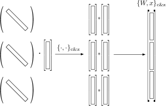
Figure 1. Dr. of Crosswise. Visual description of $\mathop{\rm c\&z}\nolimits$.

These products between matrices have useful properties:

$$(A\otimes B)(C\otimes D)=AC\otimes BD$$ (7)

$$(A\otimes B)^{\dagger}=A^{\dagger}\otimes B^{\dagger}$$ (8)

$$A\odot B\odot C=(A\odot B)\odot C=A\odot(B\odot C)$$ (9)

$$(A\odot B)^{T}(A\odot B)=A^{T}A*B^{T}B$$ (10)

$$(A\odot B)^{\dagger}=((A^{T}A)*(B^{T}B))^{\dagger}(A\odot B)^{T}$$ (11)

where $\odot$ denotes KHATRI RAO product, $\otimes$ specifies KRONECKER product and $*$ means HADAMARD product. $A\dagger$ is the MOORE PENROSE pseudo-inverse of $A$.

Take special note on the fact that for example, to transform an input vector of size $4$, to an output vector of size $8$, in the standard formulation of Neural Networks we have to learn $32$ weights. If we consider Dr. of Crosswise, the number of learned parameters to do exactly the same operation reduces to $8$. More importantly, the number of multiplications and additions also drastically lowers.

4. Rationale

We start with an exordium on Kernel Methods Cortes and Vapnik [1995]; Vapnik and Izmailov [2018]. Let $X$ be a measure space with $k:L^{2}(X\times X)\to\mathbb{R}$. We name $k$ a kernel if, and only if, there is some feature map $\phi:X\to\mathbb{H}$ into a separable HILBERT space $\mathbb{H}$ such that

$$k(x,x^{\prime})=\langle\phi(x),\phi(x^{\prime})\rangle_{\mathbb{H}}.$$ (12)

In other words, $k$ is a kernel if, and only if, for some space $\mathbb{H}$ and map $\phi$ the following diagram commutes:

Random Kitchen Sinks Rahimi and Recht [2007] approximate this mapping of features $\phi$ by a FOURIER expansion in the case of RBF kernels

$$k(x,x^{\prime})=\int\exp{(i\langle w,x\rangle)}\exp{(-i\langle w,x^{\prime}\rangle)}d\rho(w).$$ (13)

Le et al. [2013]; Yang et al. [2014] present a fast approximation of the matrix $W$. Recent works on the matter Wu et al. [2016]; Yang et al. [2015]; Moczulski et al. [2016]; Hong et al. [2017] use this technique to extract meaningful features.

Dr. of Crosswise is motivated by the construction McKernel in Curtó et al. [2017b], where Deep Learning and Kernel Methods are unified by extending the use of the approximation of $W$, $\hat{Z}$, to a SGD optimization setting

$$\hat{Z}:=\frac{1}{\sigma\sqrt{n}}CHG\Pi HB.$$ (14)

Here $C,G$ and $B$ are matrices diagonal, $\Pi$ is a random matrix of permutation and $H$ is the Hadamard. Whenever the number of rows in $W$ exceeds the dimensionality of the data, simply generate multiple instances of $\hat{Z}$, drawn i.i.d., until the required number of dimensions is obtained.

The key idea behind it is that the FOURIER transform diagonalizes the integral operator.

This can be best seen as follows. Considering the operator of convolution working on the complex exponential $f(z)=\exp(ikz)$

$$g(z)=(f*r)(z)=\int_{-\infty}^{\infty}f(\tau)r(z-\tau)d\tau.$$ (15)

Then

$$g(z)=\lambda f(z)$$ (16)

where $\lambda=R(k)$ and $R$ is the FOURIER transform of $r$.

We build on these ideas to pioneer a framework of Deep Learning where the formalism used entangles matrices diagonal.

References

- [1]
- Acuna et al. [2018] D. Acuna, H. Ling, A. Kar, and S. Fidler. 2018. Efficient Interactive Annotation of Segmentation Datasets with Polygon-RNN++. CVPR (2018).
- Bengio and Frasconi [1993] Y. Bengio and P. Frasconi. 1993. Credit Assignment through Time: Alternatives to Backpropagation. NIPS (1993).
- Coleman et al. [2017] C. Coleman, D. Narayanan, D. Kang, T. Zhao, J. Zhang, L. Nardi, P. Bailis, K. Olukotun, C. Ré, and M. Zaharia. 2017. DAWNBench: An End-to-end Deep Learning Benchmark and Competition. NIPS (2017).
- Cortes et al. [2017] C. Cortes, X. Gonzalvo, V. Kuznetsov, M. Mohri, and S. Yang. 2017. AdaNet: Adaptive Structural Learning of Artificial Neural Networks. ICML (2017).
- Cortes and Vapnik [1995] C. Cortes and V. Vapnik. 1995. Support Vector Networks. Machine Learning (1995).
- Cubuk et al. [2018] E. D. Cubuk, B. Zoph, D. Mane, V. Vasudevan, and Q. V. Le. 2018. AutoAugment: Learning Augmentation Policies from Data. arXiv:1805.09501 (2018).
- Curtó et al. [2017a] J. D. Curtó, I. C. Zarza, F. Torre, I. King, and M. R. Lyu. 2017a. High-resolution Deep Convolutional Generative Adversarial Networks. arXiv:1711.06491 (2017).
- Curtó et al. [2017b] J. D. Curtó, I. C. Zarza, F. Yang, A. Smola, F. Torre, C. W. Ngo, and L. Gool. 2017b. McKernel: A Library for Approximate Kernel Expansions in Log-linear Time. arXiv:1702.08159 (2017).
- Devlin et al. [2018] J. Devlin, M. Chang, K. Lee, and K. Toutanova. 2018. BERT: Pre-training of Deep Bidirectional Transformers for Language Understanding. arXiv:1810.04805 (2018).
- Duan et al. [2016] Y. Duan, X. Chen, R. Houthooft, J. Schulman, and P. Abbeel. 2016. Benchmarking Deep Reinforcement Learning for Continuous Control. ICML (2016).
- Girshick [2015] R. Girshick. 2015. FAST R-CNN. ICCV (2015).
- Goodfellow et al. [2014] I. Goodfellow, J. Pouget-Abadie, M. Mirza, B. Xu, D. Warde-Farley, S. Ozair, A. Courville, and Y. Bengio. 2014. Generative Adversarial Neworks. NIPS (2014).
- He et al. [2017] K. He, G. Gkioxari, P. Dollár, and R. Girshick. 2017. MASK R-CNN. ICCV (2017).
- He et al. [2016] K. He, X. Zhang, S. Ren, and J. Sun. 2016. Deep Residual Learning for Image Recognition. CVPR (2016).
- Hong et al. [2017] W. Hong, J. Yuan, and S. D. Bhattacharjee. 2017. Fried Binary Embedding for High-dimensional Visual Features. CVPR (2017).
- Karras et al. [2018] T. Karras, T. Aila, S. Laine, and J. Lehtinen. 2018. Progressive Growing of GANs for Improved Quality, Stability, and Variation. ICLR (2018).
- Kolda and Bader [2009] T. G. Kolda and B. W. Bader. 2009. Tensor Decompositions and Applications. SIAM (2009).
- Le et al. [2013] Q. Le, T. Sarlós, and A. Smola. 2013. Fastfood - Approximating Kernel Expansions in Loglinear Time. ICML (2013).
- Lecun et al. [1998] Y. Lecun, L. Bottou, Y. Bengio, and P. Haffner. 1998. Gradient-based Learning Applied to Document Recognition. Proceedings of the Institute of Electrical and Electronics Engineers (1998).
- Levine et al. [2016] S. Levine, C. Finn, T. Darrell, and P. Abbeel. 2016. End-to-end Training of Deep Visuomotor Policies. JMLR (2016).
- Long et al. [2014] J. Long, E. Shelhamer, and T. Darrell. 2014. Fully Convolutional Networks for Semantic Segmentation. CVPR (2014).
- Mhaskar et al. [2017] H. Mhaskar, Q. Liao, and T. Poggio. 2017. When and Why Are Deep Networks Better than Shallow Ones? AAAI (2017).
- Mikolov et al. [2013] T. Mikolov, I. Sutskever, K. Chen, G. Corrado, and J. Dean. 2013. Distributed Representations of Words and Phrases and their Compositionality. NIPS (2013).
- Moczulski et al. [2016] M. Moczulski, M. Denil, J. Appleyard, and N. Freitas. 2016. ACDC: A Structured Efficient Linear Layer. ICLR (2016).
- Pennington et al. [2014] J. Pennington, R. Socher, and C. D. Manning. 2014. GloVe: Global Vectors for Word Representation. EMNLP (2014).
- Poggio et al. [2017] T. Poggio, H. Mhaskar, L. Rosasco, B. Miranda, and Q. Liao. 2017. Why and When Can Deep-but not Shallow-networks Avoid the Curse of Dimensionality: A Review. International Journal of Automation and Computing (2017).
- Radford et al. [2016] A. Radford, L. Metz, and S. Chintala. 2016. Unsupervised Representation Learning with Deep Convolutional Generative Adversarial Network. ICLR (2016).
- Rahimi and Recht [2007] A. Rahimi and B. Recht. 2007. Random Features for Large-scale Kernel Machines. NIPS (2007).
- Rahimi and Recht [2008] A. Rahimi and B. Recht. 2008. Weighted Sums of Random Kitchen Sinks: Replacing Minimization with Randomization in Learning. NIPS (2008).
- Ren et al. [2015] S. Ren, K. He, R. Girshick, and J. Sun. 2015. FASTER R-CNN: Towards Real-time Object Detection with Region Proposal Networks. NIPS (2015).
- Salimans et al. [2016] T. Salimans, I. Goodfellow, W. Zaremba, V. Cheung, A. Redford, and X. Chen. 2016. Improved Techniques for Training GANs. NIPS (2016).
- Simonyan and Zisserman [2015] K. Simonyan and A. Zisserman. 2015. Very Deep Convolutional Networks For Large-scale Image Recognition. ICLR (2015).
- Tremblay et al. [2018] J. Tremblay, A. Prakash, D. Acuna, M. Brophy, V. Jampani, C. Anil, T. To, E. Cameracci, S. Boochoon, and S. Birchfield. 2018. Training Deep Networks with Synthetic Data: Bridging the Reality Gap by Domain Randomization. CVPR (2018).
- Vapnik and Izmailov [2018] V. Vapnik and R. Izmailov. 2018. Rethinking Statistical Learning Theory: Learning Using Statistical Invariants. Machine Learning (2018).
- Wu et al. [2016] L. Wu, I. E. H. Yen, J. Chen, and R. Yan. 2016. Revisiting Random Binning Features: Fast Convergence and Strong Parallelizability. KDD (2016).
- Yang et al. [2015] Z. Yang, M. Moczulski, M. Denil, N. Freitas, A. Smola, L. Song, and Z. Wang. 2015. Deep Fried Convnets. ICCV (2015).
- Yang et al. [2014] Z. Yang, A. Smola, L. Song, and A. G. Wilson. 2014. À la Carte - Learning Fast Kernels. AISTATS (2014).
- Yu and Koltun [2016] F. Yu and V. Koltun. 2016. Multi-scale Context Aggregation by Dilated Convolutions. ICLR (2016).