Inverse cascade of hybrid helicity in $B\Omega$-MHD turbulence

Abstract

We investigate the impact of a solid-body rotation $\bm{\Omega}_{0}$ on the large-scale dynamics of an incompressible magnetohydrodynamic turbulent flow in presence of a background magnetic field ${\bf B_{0}}$ and at low Rossby number. Three-dimensional direct numerical simulations are performed in a periodic box, at unit magnetic Prandtl number and with a forcing at intermediate wavenumber $k_{f}=20$. When $\bm{\Omega}_{0}$ is aligned with ${\bf B_{0}}$ (i.e. $\theta\equiv\widehat{\left(\bm{\Omega}_{0},{\bf B_{0}}\right)}=0$), inverse transfer is found for the magnetic spectrum at $k<k_{f}$. This transfer is stronger when the forcing excites preferentially right-handed (rather than left-handed) fluctuations; it is smaller when $\theta>0$ and becomes weak when $\theta\geq 35^{o}$. These properties are understood as the consequence of an inverse cascade of hybrid helicity which is an inviscid/ideal invariant of this system when $\theta=0$. Hybrid helicity emerges, therefore, as a key element for understanding rotating dynamos. Implication of these findings on the origin of the alignment of the magnetic dipole with the rotation axis in planets and stars is discussed.

I Introduction

Table 1: Main parameters of the simulations cited in the text. From left to right we find the name of the simulation, the amplitudes of the rotation rate and of the uniform magnetic field, the hypoviscosity, the normalized cross-correlation, the angle $\theta\equiv\widehat{\left(\bm{\Omega}_{0},{\bf B_{0}}\right)}$, the Rossby number, the Reynolds number and the time at which the simulation has been stopped. All the simulations have been performed with a resolution $N=256^{3}$ for a box size $L=2\pi$, a reduced magnetic helicity $\sigma_{m}=0.5$ and a viscosity $\nu^{+}=\eta^{+}=2.10^{-3}$.

Simulation	$\Omega_{0}$	$B_{0}$	$\nu^{-}=\eta^{-}$	$\sigma_{c}$	$\theta$	$Ro$ ($10^{-3}$)	$Re$	$t_{f}$
20L	$20$	$1$	$0$	$0.5$	$0$	$1.54$	$1215$	$69$
20R	$20$	$1$	$0$	$-0.5$	$0$	$1.5$	$1182$	$69$
0R	$0$	$1$	$0$	$-0.5$	$0$	$\infty$	$1344$	$62$
20R_B0	$20$	$0$	$0$	$-0.5$	$0$	$1.45$	$1147$	$97$
$\bf 20R_{0}$	$20$	$1$	$2.10^{-2}$	$-0.5$	$0$	$1.49$	$1176$	$133$
$\bf 20R_{25}$	$20$	$1$	$2.10^{-2}$	$-0.5$	$25$	$1.49$	$1175$	$105$
$\bf 20R_{35}$	$20$	$1$	$2.10^{-2}$	$-0.5$	$35$	$1.47$	$1163$	$113$
$\bf 20R_{45}$	$20$	$1$	$2.10^{-2}$	$-0.5$	$45$	$1.49$	$1178$	$117$
$\bf 20R_{90}$	$20$	$1$	$2.10^{-2}$	$-0.5$	$90$	$1.57$	$1241$	$108$

The emergence of large-scale magnetic fields in various astrophysical objects (like planets, stars, accretion discs or galaxies) is mainly attributed to a dynamo mechanism based on the turbulent motions of a conducting fluid described by magnetohydrodynamics (MHD) Moffatt (1972); Brandenburg and Subramanian (2005); Kulsrud and Zweibel (2008); Galtier (2016); Moutou et al. (2017). Because the magnetic flux is conserved in ideal MHD, the stretching of magnetic field lines by the conducting fluid can amplify magnetic fluctuations at small scales. It is thought that these turbulent fluctuations are then transported to large-scales via an inverse cascade of magnetic helicity Frisch et al. (1975); Pouquet et al. (1976); Pouquet and Patterson (1978); Meneguzzi et al. (1981); Alexakis et al. (2006), which is an ideal invariant of three-dimensional (3D) MHD Woltjer (1958). The presence of inverse transfer of magnetic energy in absence of magnetic helicity is also possible as pointed out in Brandenburg et al. (2015) (see also Gilbert et al. (1988); Urpin (2002); Tobias and Cattaneo (2013)). This transfer is, however, weaker than the one found with magnetic helicity and could be explained e.g. by the form of the initial spectrum in the sub-inertial range Olesen (1997).

Strictly speaking, direct and inverse cascades are expected only for quantities which are invariant of a system in the non-dissipative case, whatever the turbulence regime (strong or weak) Frisch (1995); Nazarenko (2011); Banerjee and Pandit (2014); Seshasayanan et al. (2014); Alexakis and Biferale (2018). In 3D incompressible MHD, such invariants are the total energy $E$, the cross-correlation between the velocity and the magnetic field $H_{c}$, and the magnetic helicity $H_{m}$ Pouquet (1993). There are many studies devoted to the scaling of the total energy spectrum for which the answer is not unique Kraichnan (1965); Goldreich and Sridhar (1995); Galtier et al. (2000, 2005); Boldyrev (2006); Mininni and Pouquet (2007); Lee et al. (2010); Beresnyak (2014). Much less is known about the magnetic helicity while its importance is recognized e.g. in solar physics where $H_{m}$ can be measured in coronal mass ejections Priest (2014) or in the solar wind Matthaeus and Goldstein (1982). Recently, several direct numerical simulations have been devoted to the study of the magnetic helicity cascade Alexakis et al. (2006); Müller et al. (2012); Linkmann and Dallas (2016) (see also Brandenburg (2001) for compressible MHD). In particular, it is shown that the inverse cascade becomes nonlocal in wavenumber space when condensation takes place at the largest scale of the system. Under some conditions, a direct cascade of $H_{m}$ can also be found as a finite magnetic Reynolds number effect Linkmann and Dallas (2017).

The introduction of a uniform magnetic field ${\bf B_{0}}$ or the Coriolis force with a uniform rotating rate $\bm{\Omega}_{0}$ reduces the number of inviscid/ideal invariants in 3D incompressible MHD. In the first case, $H_{m}$ is no longer conserved while in the second it is $H_{c}$. When both effects are present, (situation called hereafter, $B\Omega$-MHD) the total energy remains the only invariant of the system, except if ${\bf B_{0}}$ and $\bm{\Omega}_{0}$ are aligned: in this case, there is a second invariant called hybrid helicity $H_{h}$, which is a combination of $H_{c}$ and $H_{m}$ Shebalin (2006). While analytical results have been obtained recently for weak $B\Omega$-MHD turbulence Galtier (2014) with some predictions about the hybrid helicity spectrum, no detailed numerical study has been done in the strong or weak wave turbulence regime (see, however, the recent study by Bell and Nazarenko (2019)). $B\Omega$-MHD turbulence is, however, a relevant model for studying rotating dynamos like in stars and planets which are often characterized by a magnetic dipole closely aligned with the rotation axis. The reason of this alignment is still unclear and need further investigations. Because of the complexity of the problem, only few physical ingredients are generally included in the modeling (see eg. Reshetnyak and Hejda (2008); Petitdemange (2018)). For example, we may investigate this problem by including a large-scale magnetic field ${\bf B_{0}}$ and/or a solid-body (instead of differential) rotation $\bm{\Omega}_{0}$ (see eg. Favier et al. (2012); Seshasayanan et al. (2017)).

In this article, we present a set of 3D direct numerical simulations of $B\Omega$-MHD turbulence at unit magnetic Prandtl number and low Rossby number. The investigation is focused on the large-scale dynamics (scales larger than the forcing scale). In section II we present the governing equations and the numerical setup. Section III is devoted to the numerical results. When the angle $\theta\equiv\widehat{\left(\bm{\Omega}_{0},{\bf B_{0}}\right)}$ between $\bm{\Omega}_{0}$ and ${\bf B_{0}}$ is null, we show that the magnetic spectrum exhibits a significant inverse transfer which is reduced when $\theta>0$ to become negligible for $\theta\geq 35^{o}$. We also show that this transfer is stronger when the forcing excites preferentially right-handed (rather than left-handed) fluctuations. We explain why these properties can be interpreted as the consequence of an inverse cascade of $H_{h}$, which appears as a key element to understand rotating dynamos. Finally, in section IV we present a conclusion.

II Governing equations

The equations governing incompressible $B\Omega$-MHD can be written as

$$\frac{\partial{\bf u}}{\partial t} = -\nabla P+{\bf u}\times({\bf w}+2\bm{\Omega}_{0})+(\nabla\times{\bf b})\times({\bf b}+{\bf B_{0}})$$ (1)

$$+\nu^{+}\nabla^{2}{\bf u}+\nu^{-}\nabla^{-2}{\bf u}\,,$$

$$\frac{\partial{\bf b}}{\partial t} = \nabla\times({\bf u}\times({\bf b}+{\bf B_{0}}))+\eta^{+}\nabla^{2}{\bf b}+\eta^{-}\nabla^{-2}{\bf b}\,,$$ (4)

$$\nabla\cdot{\bf u}=0\,,$$

$$\nabla\cdot{\bf b}=0\,,$$

with ${\bf u}$ the velocity, $P$ a generalized pressure, ${\bf w}=\nabla\times{\bf u}$ the vorticity and ${\bf b}$ the normalized magnetic field. $\nu^{+}$, $\eta^{+}$ and $\nu^{-}$, $\eta^{-}$ are small-scale and large-scale dissipation coefficients, respectively. We can easily check that $H_{c}$ and $H_{m}$ are not conserved in $B\Omega$-MHD since we obtain from Eqs. (1)–(4), with $\nu^{+}=\nu^{-}=\eta^{+}=\eta^{-}=0$,

$${{\color[rgb]{0,0,0}dH_{c}\over dt}} \equiv {d\over dt}\int\frac{{\bf u}\cdot{\bf b}}{2}\,d\,{\cal V}=\bm{\Omega}_{0}\cdot\int({\bf b}\times{\bf u})\,d\,{\cal V}\,,$$ (5)

$${{\color[rgb]{0,0,0}dH_{m}\over dt}} \equiv {d\over dt}\int\frac{{\bf a}\cdot{\bf b}}{2}\,d\,{\cal V}={\bf B_{0}}\cdot\int({\bf b}\times{\bf u})\,d\,{\cal V}\,,$$ (6)

where ${\bf a}$ is the vector potential (${\bf b}=\nabla\times{\bf a}$) and ${\cal V}$ a volume of integration. The hybrid helicity $H_{h}\equiv H_{m}/d-H_{c}$ with $d\equiv B_{0}/\Omega_{0}$ is, however, conserved when $\bm{\Omega}_{0}$ and ${\bf B_{0}}$ are aligned (this property is checked numerically but not shown). $d$ is called the magneto-inertial length and gives a scale of reference to measure the relative importance of the Coriolis force on the Lorentz force.

The linear solution of MHD is modified by the presence of the Coriolis force; the dispersion relation is Finlay (2008); Galtier (2014)

$$\omega=\frac{sk_{z}\Omega_{0}}{k}\left(-s\Lambda+\sqrt{1+k^{2}d^{2}}\right)\,,$$ (7)

with $k$ the wavenumber, $k_{z}$ the wavenumber component along ${\bf B_{0}}$ (here, we assume that $\bm{\Omega}_{0}$ and ${\bf B_{0}}$ are parallel), $s=\pm 1$ the directional polarity ($sk_{z}\geq 0$) and $\Lambda=\pm 1$ the wave polarization. The magnetostrophic branch ($\Lambda s=1$) and the inertial branch ($\Lambda s=-1$) correspond to the right (R) and left (L) circular polarizations, respectively. There are well separated when $kd\ll 1$ and tends to the Alfvén branch when $kd\gg 1$, also the condition $kd=1$ appears as a critical value. As shown in Galtier (2014), the polarization $P$ may be defined as ${{\color[rgb]{0,0,0}P\equiv}}\sigma_{m}\sigma_{c}=-s\Lambda$, with $\sigma_{m}$ the reduced magnetic helicity and $\sigma_{c}$ the reduced cross-correlation

$$\sigma_{m} = \frac{\hat{\bf a}\cdot\hat{{\bf b}}^{*}+\hat{\bf a}^{*}\cdot\hat{{\bf b}}}{2|\hat{\bf a}||\hat{{\bf b}}|}\,,$$ (8)

$$\sigma_{c} = \frac{\hat{{\bf u}}\cdot\hat{{\bf b}}^{*}+\hat{{\bf u}}^{*}\cdot\hat{{\bf b}}}{2|\hat{\bf u}||\hat{\bf b}|}\,,$$ (9)

where $\hat{}$ means the Fourier transform and $*$ the complex conjugate. By extension, in our numerical study we define the R and L fluctuations for which we have, respectively, $P<0$ and $P>0$. Finally note that the polarization property is lost when $\Omega_{0}=0$, while when $B_{0}=0$ we end up with a L-polarized wave, giving an asymmetric character to the dispersion relation (7).

Equations (1)–(4) are computed using a pseudo-spectral solver called TURBO Meyrand and Galtier (2012); Meyrand et al. (2016). The simulation domain is a triply periodic cube discretized by $N^{3}$ collocation points. A unit magnetic Prandtl number is taken with $\nu^{+}=\eta^{+}$; we also take $\nu^{-}=\eta^{-}$. The vector ${\bf B_{0}}$ is fixed along the z-direction while $\bm{\Omega}_{0}$ may be tilted with an angle $\theta$ in such a way that for $\theta=0$ it is also along the z-direction. The nonlinear terms are partially de-aliased using a phase-shift method. This system is forced in the Fourier space: kinetic and magnetic energy spectra are excited at wavenumbers $19\leq k_{f}\leq 21$ with a rate of injection $\epsilon_{u}$ and $\epsilon_{b}$, respectively, while there is no injection of kinetic helicity Teaca et al. (2011). We take $\epsilon_{u}=\epsilon_{b}=0.2$ for all simulations. Magnetic helicity and cross-correlation are also injected at $k_{f}$ with a reduced rate $\sigma_{m}$ and $\sigma_{c}$, respectively. We take $\sigma_{m}=0.5$, then the sign of $\sigma_{c}$ will determine the polarization (left or right). In real systems this type of polarized forcing may find its origin in the excitation of magnetostrophic or inertial waves preferentially (see eg. Le Reun et al. (2017)). Note that the simulations have been stopped at a time $t_{f}\gg t_{NL}\sim 1$, where $t_{NL}$ is the nonlinear time, i.e. the time needed to form the small-scale ($k>k_{f}$) spectra. Therefore, the dynamics that we investigate is relatively slow and requires a long numerical computation.

A summary of the different simulations is given in Table 1. In particular, the choice of $\Omega_{0}$ and $B_{0}$ is made to keep $k_{f}d=1$. Simulations have been computed to obtain a sufficiently large steady state window for the kinetic energy (with a steady state that starts at $t_{steady}\sim 40$ for cases 20L, 20R, 0R and $t_{steady}\sim 80$ for all the others). The Rossby, $Ro=U/(2\Omega_{0}L)$, and Reynolds, $Re=UL/\nu^{+}$, numbers are calculated from the root mean square value of the velocity field averaged over the entire volume $V$ of the numerical box and time-averaged for $t_{steady}\leq t\leq t_{f}$: $U=\langle\langle{\bf u}\cdot{\bf u}\rangle_{V}\rangle_{t}^{1/2}$.

III Results

III.1 Impact of the circular polarizations

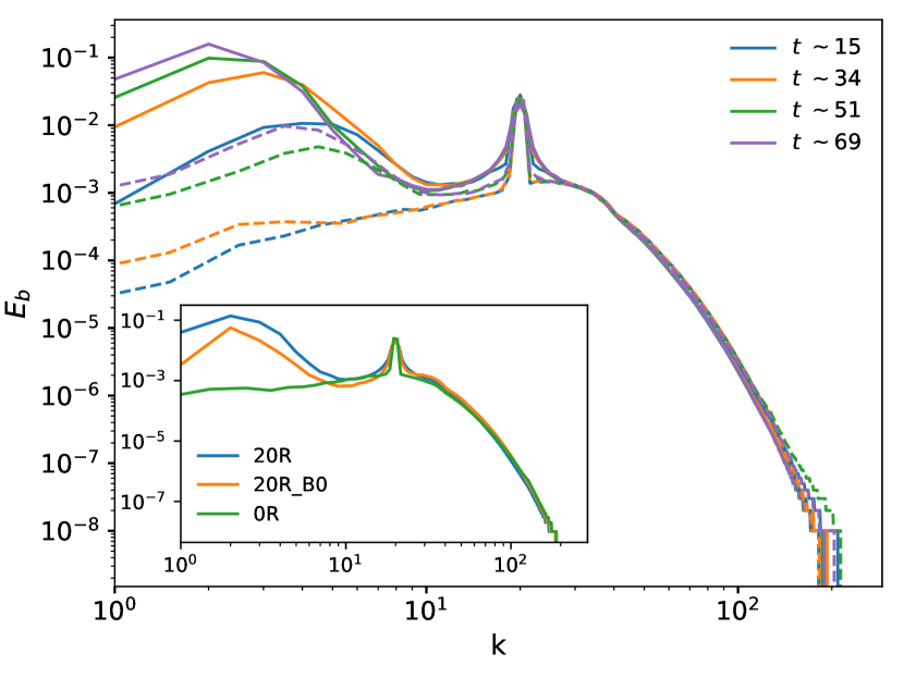
Figure 1: Temporal evolution of the magnetic spectrum for simulations 20R (solid line) and 20L (dashed line). The parameters of these simulations can be found in Table 1. Colors indicate the approximate times at which the spectra have been computed. Note that simulation 20R is stopped before the formation of a condensate. Insert: spectrum of case 20R at $t\sim 62$ compared with two reference cases: without rotation (case 0R) and without magnetic field (case 20R_B0).

$B\Omega$-MHD turbulence is characterized by two types of fluctuations (R and L). We start our analysis by studying the impact on the large-scale dynamics of a forcing which excites preferentially the R (simulation 20R) or the L (simulation 20L) fluctuations. Both magnetic $E_{b}$ and kinetic $E_{u}$ energies spectra have been calculated to diagnose the dynamics, however, $E_{u}$ is nearly constant for these two cases. The behavior of the kinetic energy will be briefly discussed in section III.2. Fig. 1 shows the results with the time evolution of the magnetic spectrum. The plots are given for approximately the same times. The simulation 20R is stopped before the formation of a condensate at low wave numbers which may have an impact on the dynamics (finite box effect). In both cases inverse transfers of magnetic energy are found for $k<k_{f}$, however, we clearly see that the efficiency of the transfer is greater when the R-fluctuations are preferentially excited: the magnetic energy transfer to large scales occurring in case 20L (dashed line) is considerably less efficient than in case 20R as the maximum value reached by the magnetic energy at the final time $t\sim 69$ differs by more than an order of magnitude. This difference can be understood by using wave turbulence arguments: the dynamics of the R-fluctuations is mainly driven by the magnetic field while it is mainly driven by the velocity field for the L-fluctuations Galtier (2014). Therefore, simulation 20R (solid line) strengthens a dynamics driven by the magnetic field. The efficiency of this transfer is also compared (see insert) to a rotating case without magnetic field (simulation 20R_B0). The same behavior is observed, however, we see that adding a mean magnetic field to the strong rotation enhances slightly the inverse transfer of magnetic energy. The situation is quite different when we remove the rotation (simulation 0R): in this case the fluctuations are not circularly polarized, the large-scale magnetic spectrum is flat and does not evolve very much.

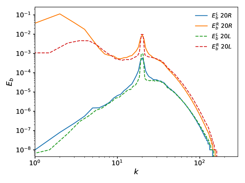
Figure 2: Magnetic spectra at $t\sim 69$ for simulations 20R (solid line) and 20L (dashed line) decomposed into L ($E^{L}_{b}$) and R ($E^{R}_{b}$) fluctuations. This decomposition highlights the relative importance of each type of fluctuations in a single simulation.

Fig. 2 confirms the first picture by showing the spectra of Fig. 1 but only for the final times and decomposed into L- and R-fluctuations (the decomposition is discussed in Galtier (2014); see also Appendix A). For both simulations we see that the inverse cascade involves mainly the R-fluctuations and these fluctuations are larger for simulation 20R: the R-fluctuations drive the mechanism of inverse transfer in both simulations, whereas the L-fluctuations are significantly smaller at large scales. This difference can be explained as the condition $k_{f}d=1$ leads to a magnetostrophic regime (R polarization) at large scales ($k<k_{f}$). As expected, the efficiency of a L-type forcing (dashed line on Fig. 2) to drive an inverse cascade of magnetic energy is significantly weaker than for a R-type forcing (solid line on Fig. 2). Note that a similar analysis was performed for studying Hall MHD turbulence where a different behavior was also found for the L and R magnetic fluctuations spectra Meyrand and Galtier (2012).

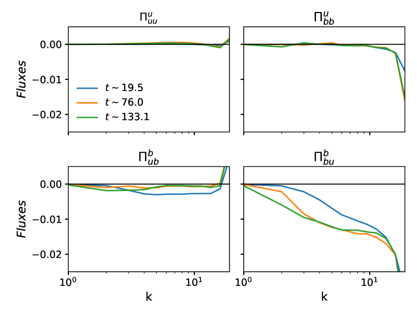
Figure 3: Spectral flux (in logarithmic-linear coordinates) associated with the four different nonlinear terms of $B\Omega$-MHD (simulation 20R) for three typical times. The main contribution exhibiting a significant negative flux at large scales ($k<k_{f}$) comes from $\Pi^{b}_{bu}$.

In Fig. 3 we plot in the spectral space (for simulation 20R) the contributions of the four different terms of $B\Omega$-MHD to the total energy flux as derived by Dar et al. (2001) and Verma (2004) for $k<k_{f}$ only. We used the notation $\Pi^{X}_{YZ}(k)$ for a flux from inside the shell $k$ of the field X to outside the shell $k$ of field Z via field Y. By definition Frisch (1995); Dar et al. (2001); Verma (2004); Seshasayanan and Alexakis (2016); Kumar and Verma (2017); Meyrand et al. (2018), we have:

$$\Pi^{u}_{uu}(k) = {\bf u}_{k}^{<}\cdot({\bf u}\cdot\nabla{{\color[rgb]{0,0,0}{\bf u}_{k}^{>}}})\,,$$ (10)

$$\Pi^{u}_{bb}(k) = -{\bf u}_{k}^{<}\cdot({\bf b}\cdot\nabla{{\color[rgb]{0,0,0}{\bf b}_{k}^{>}}})\,,$$ (11)

$$\Pi^{b}_{ub}(k) = {\bf b}_{k}^{<}\cdot({\bf u}\cdot\nabla{{\color[rgb]{0,0,0}{\bf b}_{k}^{>}}})\,,$$ (12)

$$\Pi^{b}_{bu}(k) = -{\bf b}_{k}^{<}\cdot({\bf b}\cdot\nabla{{\color[rgb]{0,0,0}{\bf u}_{k}^{>}}})\,,$$ (13)

where ${\bf u}_{k}^{<}$ is the filtered velocity (or magnetic field ${\bf b}_{k}^{<}$) so that only the modes $|{\bf k}|<k$ are being kept. While the contribution from the advection term $\Pi^{u}_{uu}$ has the smallest amplitude, we see that the main contribution to the negative flux at large scales ($k<k_{f}$) comes from $\Pi^{b}_{bu}$. Although the range of scales is narrow, a plateau seems to emerge with time. We also see that there is a non negligible contribution of flux $\Pi^{b}_{ub}$ with a negative value. These two fluxes come from the induction equation, which is consistent with our interpretation (a dynamics dominated by the magnetic field). The fluxes at $k_{f}>20$ (not presented) have a classical positive and decreasing shape from the forcing wave numbers to the dissipative scales, signature of a direct cascade.

III.2 Impact of a tilted rotation axis

The hybrid helicity is an invariant of non-dissipative $B\Omega$-MHD only when $\theta=0^{o}$. Here, we study the impact of this angle on the large-scale dynamics. For this study, a hypoviscosity term has been added ($\nu_{-}\neq 0$; see Table 1) to avoid the condensation observed in section III.1 and the finite box effects at small wavenumber. We will assume for the moment that $H_{h}$ is mainly driven by the magnetic helicity (see Fig. 8 for a justification). Fig. 4 shows the results for five different angles. The same forcing as in simulation 20R is applied. A significant decrease of the inverse transfer is observed when the angle $\theta$ increases. For $\theta=90^{o}$ the transfer can be qualified as negligible. This property of $B\Omega$-MHD turbulence can be interpreted as the direct consequence of the non conservation of $H_{h}$: the large-scale dynamics observed for $\theta=0^{o}$ is explained by the inverse cascade of $H_{h}$ which decreases when $\theta>0^{o}$. Whereas from a theoretical point of view we expect the absence of inverse cascade as soon as $\theta>0^{o}$, Fig. 4 reveals the existence of a gradual decrease of this cascade. Moreover, the large scale behavior differs when $\theta\geq 45^{o}$ with the presence of a significant peak at wavenumber $k=2$ and a curve instead of power law for $k>2$. Further analysis reveals that this behavior seems correlated with that of $E_{u}$.

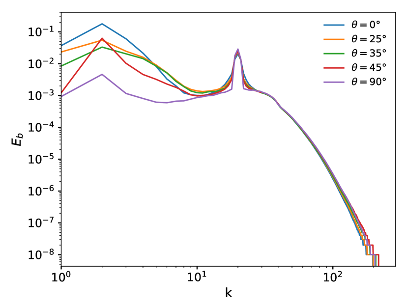
Figure 4: Magnetic spectra for situations where the angles $\theta=0^{o},25^{o},35^{o},45^{o}$ and $90^{o}$ (simulations 20R₀ to 20R₉₀). The spectra are plotted approximately at the same time $t\sim 105$. Hypoviscosity ($\nu^{-}$) has been added to avoid a condensation at small $k$. At large scales, a similar shape is observed for $\theta\leq 35^{o}$ whereas the behavior seems different when $\theta\geq 45^{o}$.

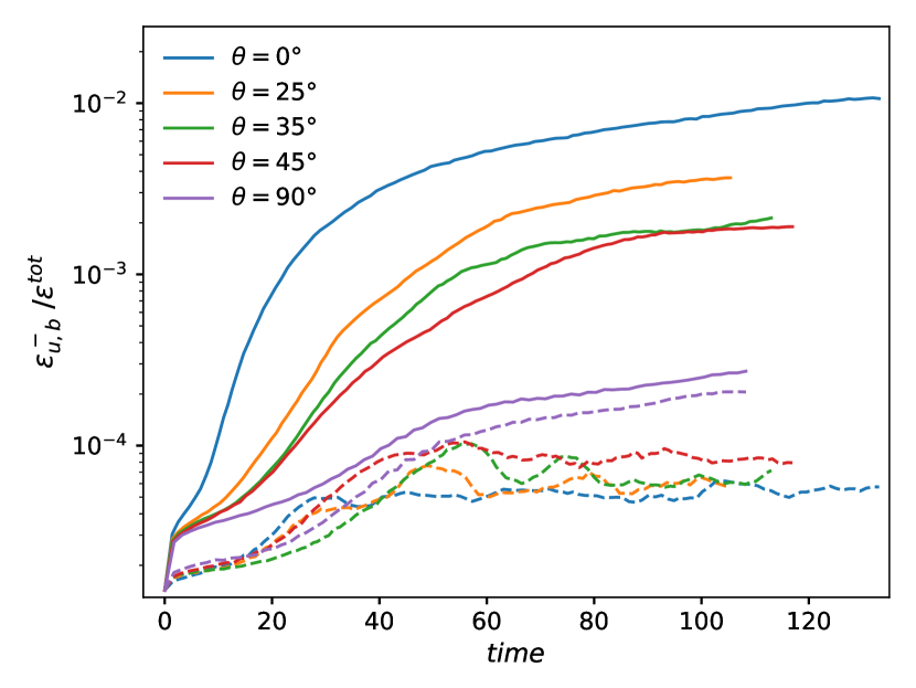
Figure 5: Time evolution (in linear-logarithmic scales) of the normalized large-scale dissipation rate of kinetic energy $\epsilon^{-}_{u}$ (dashed lines) and magnetic energy $\epsilon^{-}_{b}$ (solid lines) for angles $\theta=0^{o}$, $25^{o}$, $35^{o}$, $45^{o}$ and $90^{o}$. $\epsilon^{tot}\equiv\epsilon^{+}+\epsilon^{-}$ is the total dissipation rate. For $\theta=0^{o}$ the large scale dissipation rate is dominated by the magnetic contribution, while for $\theta=90^{o}$ the contribution of each field is similar.

A better way to quantify this evolution is to measure the dissipation rate of energy at small and large scales

$$\epsilon^{\pm}=\nu^{\pm}\sum_{{\bf k}\neq{\bf 0}}k^{\pm 2}(|\hat{{\bf u}}|^{2}+|\hat{{\bf b}}|^{2})=\epsilon^{\pm}_{u}+\epsilon^{\pm}_{b}\,.$$ (14)

In particular, $\epsilon^{-}_{u,b}/(\epsilon^{+}+\epsilon^{-})$ provides a measure of the strength of the inverse cascade Seshasayanan et al. (2014). Note that this measure does not require a mechanism of inverse cascade driven by the total energy. Fig. 5 displays the result for five angles. For $\theta=0^{o}$ we see that the fast growth of the large-scale magnetic dissipation observed initially is followed by a phase of slow growth meaning that the stationary state is only reached approximately. Interestingly the value obtained at the final time of the simulation is around $10^{-2}$, which means that most of the magnetic energy flux goes to small-scales, a property expected because of the direct energy cascade. The comparison with the other angles reveals a significant decrease of the large-scale magnetic dissipation and a slight increase of the large-scale kinetic dissipation. For $90^{o}$ an equipartition of the dissipation rates is almost reached. In this case the magnetic and kinetic energy spectra become very close (not shown). It is interesting to note that this tendency to the equipartition for $\theta=90^{o}$ can be predicted already at the level of a linear analysis Salhi et al. (2017). In conclusion, this new diagnostic confirms the analysis made from Fig. 4 but in addition we can claim that the strength of the inverse cascade becomes significantly weaker (about an order of magnitude) when $\theta\geq 35^{o}$.

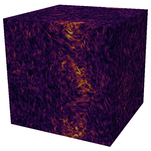
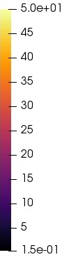
Figure 6: Amplitude of the current density for case $20R_{0}$ at $t\sim 105$. The magnetic field is along ${\bf z}$, corresponding to the vertical axis on this representation. Despite strong rotation, no strong anisotropy is observed.

The amplitude of the current density is shown on Fig. 6 for the reference case $\theta=0^{o}$ in 3D-space with the vertical axis corresponding to ${\bf z}$. Despite the strong rotation imposed, there is no evidence for a strong anisotropy along the $\Omega_{0}$ direction. Especially no columnar structures leading to a quasi-2D turbulence are observed like for a purely rotational case (see eg. Sharma et al. (2018)) or a purely magnetic case (see eg. Sundar et al. (2017)) where, however, hypoviscosity/hyporesistivity was not introduced. By comparing their results to our similar cases (respectively 20R_B0 and 0R), this quasi-2D behavior is not observed neither. This difference can be explained by different parameter ranges and also by a wave-type forcing which may prevent the formation of coherent structures. Vorticity field for the same simulation is pretty similar and therefore not shown. Note that no structures are observed when the rotation axis is tilted.

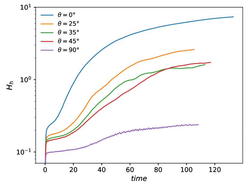
Figure 7: Time evolution (in linear-logarithmic scales) of the hybrid helicity $H_{h}$ for the five simulations with different values of $\theta$. Note that the particular behaviors of case $20R_{35}$ and $20R_{45}$ which cross around $t=90$ seem to have different origins (see Fig. 4). As expected, $H_{h}$ is much smaller for the orthogonal configuration $20R_{90}$.

Fig. 7 shows the time evolution of the hybrid helicity with respect to $\theta$. We do not expect the conservation of this quantity in this case since an external forcing is applied. However, a stationary state may be reached in presence of hypoviscosity because of the balance between forcing and dissipation. Although the final times $t_{f}$ of the simulations are not exactly the same we see a general tendency with an accumulation of hybrid helicity into the system as a consequence of the inverse cascade. More than an order of magnitude of difference is found at $t_{f}$ between angles $\theta=0^{o}$ and $90^{o}$. The figure also shows that a stationary state is reached only approximately. Finally, note that the curves at $\theta=35^{o}$ and $45^{o}$ intersect around $t=90$. This observation has to be compared with the spectral behavior found in Fig. 4 at wavenumber $k=2$ to understand that the large scale repartition of energy is different.

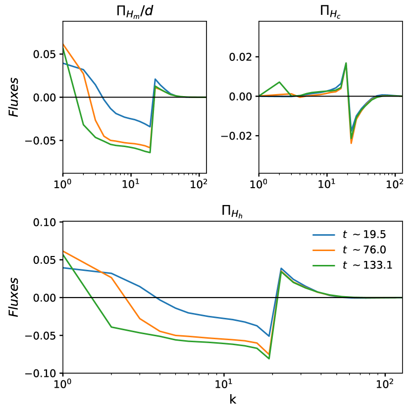
Figure 8: Spectral fluxes (in logarithmic-linear scales) of the normalized magnetic helicity (top left) divided by $d$, cross-correlation (top right) and hybrid helicity (bottom) for simulation 20R₀ at three different times. The hybrid helicity and the magnetic helicity exhibit a plateau at large scale which widens with time.

To further investigate the dynamics of the hybrid helicity we define the following fluxes

$$\Pi_{H_{m}}(k) = -{\bf b}_{k}^{<}\cdot({\bf u}\times{{\color[rgb]{0,0,0}{\bf b}_{k}^{>}}})\,,$$ (15)

$$\Pi_{H_{c}}(k) = \frac{1}{2}[{\bf b}_{k}^{<}\cdot({\bf u}\cdot\nabla{{\color[rgb]{0,0,0}{\bf u}_{k}^{>}}}-{\bf b}\cdot\nabla{{\color[rgb]{0,0,0}{\bf b}_{k}^{>}}})$$ (16)

$$+{\bf u}_{k}^{<}\cdot({\bf u}\cdot\nabla{{\color[rgb]{0,0,0}{\bf b}_{k}^{>}}}-{\bf b}\cdot\nabla{{\color[rgb]{0,0,0}{\bf u}_{k}^{>}}})]\,,$$

$$\Pi_{H_{h}}(k) = \Pi_{H_{m}}(k)/d-\Pi_{H_{c}}(k)\,,$$ (17)

for the magnetic helicity, the cross-correlation and the hybrid helicity, respectively. The time evolution of these spectra is shown in Fig. 8 for $\theta=0^{o}$. This figure provides an additional information: the hybrid helicity spectrum (bottom) tends to be formed with a constant negative flux at large scales. This negative flux can be attributed to the magnetic helicity (top left) whereas the cross-helicity displays only a slight positive flux (top right). It is important to note that unlike total energy, the quantities $H_{m}$, $H_{c}$ and $H_{h}$ are not positive defined. However, since the forcing excites preferentially the right fluctuations it is expected to have a positive magnetic helicity (as we checked). Since $H_{m}/d$ has a dominant contribution to $H_{h}$ our interpretation about the sign of the hybrid helicity flux is therefore probably correct. Note that a positive flux at the largest scales is also observed in other studies and usually interpreted as an effect of the periodic boundaries of the numerical box.

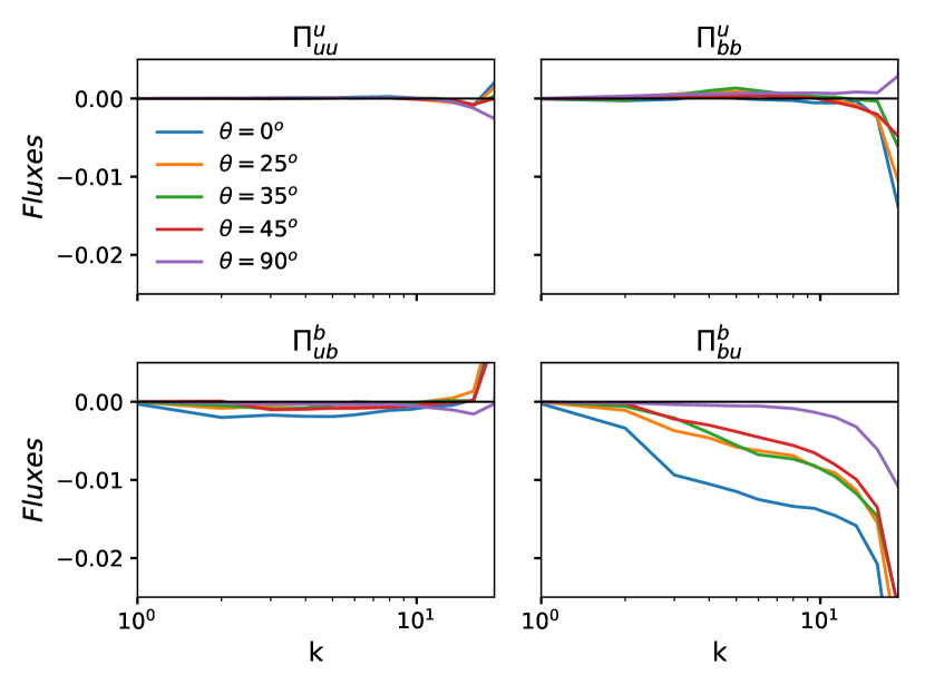
Figure 9: Spectral fluxes (in logarithmic-linear scales) associated with the four different nonlinear terms of $B\Omega$-MHD for several angles (simulation $20R_{0}$ to $20R_{90}$) and at time $t\sim 105$. For the flux $\Pi^{b}_{bu}$, the difference between $\theta=0^{o}$ and the other angles is undeniable.

In Fig. 9 we see how the angle $\theta$ affects the flux associated with the four different nonlinear terms of $B\Omega$-MHD. The most remarkable evolution comes from the bottom-right panel where the main driver of the inverse cascade is plotted: its flux is drastically reduced when $\theta$ increases. The inverse transfer is almost completely damped for a large $\theta$ angle.

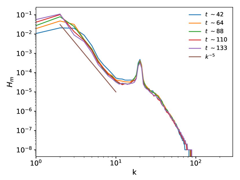
Figure 10: Time evolution of the magnetic helicity spectrum for simulation $20R_{0}$. The spectra are compared with a power law in $k^{-5}$ (segment). Note that the spectrum peaks at wavenumber $k=2$ from $t\sim 88$.

Finally, the time evolution of the magnetic helicity spectrum is shown in Fig. 10 for $\theta=0^{o}$ (simulation $20R_{0}$). As we see the large scale spectrum is well fitted with a power law in $k^{-5}$. Even if a power law is found in a narrow wavenumber window we may try to compare it with theoretical predictions. The law found is quite different from the pure MHD case ($\Omega_{0}=B_{0}=0$) where a direct numerical simulations showed a $k^{-3.6}$ scaling Müller et al. (2012) or for which a closure model predicted a $k^{-2}$ scaling Pouquet et al. (1976). It is also different from the weak wave turbulence prediction Galtier (2014). Therefore, the spectrum observed remains unexplained.

IV Conclusion

The present study was focused on the impact of a polarized forcing at intermediate scale on the large-scale dynamics of $B\Omega$-MHD turbulence at low Rossby number. The main property found is that a right-handed polarization is much more efficient than a left-handed to excite large-scale magnetic field fluctuations. This can be explained by invoking wave turbulence arguments and the hybrid helicity $H_{h}$ which is a conserved quantity when the rotation axis $\bm{\Omega}_{0}$ and the background magnetic field ${\bf B_{0}}$ are aligned. As a consequence of this inviscid property we observe an inverse cascade of $H_{h}$ with a constant negative flux. This inverse transfer decreases when the angle $\theta\equiv\widehat{\left(\bm{\Omega}_{0},{\bf B_{0}}\right)}>0^{o}$; it becomes weak when $\theta\geq 35^{o}$. This critical angle is, however, not universal and could be smaller when right- and left-handed fluctuations are equally excited.

Stars and planets are often characterized by a magnetic dipole closely aligned with the rotation axis. Why ? The answer to this question is far from trivial because it involves many sub-questions linked to the turbulent dynamo problems in a spherical geometry. Usually because of the complexity of the problem, only few physical ingredients are included in the modeling like the thermal convection and the rotation which can be simplified by considering a solid-body instead of a differential rotation. Furthermore, the magnetic Prandtl number $P_{m}$ can take very different values if one considers stars or planet interiors but generally in both cases $P_{m}<1$. Last but not least, the conducting fluid is highly turbulent and requires power numerical resources if one wants to find solutions that cover a wide range of scales.

Our study reveals that the regeneration of a large-scale magnetic field can be done through an inverse cascade of hybrid helicity. We found that the inverse cascade is more efficient when the angle $\theta$ is small. This result is an indication that the dynamo mechanism is more efficient when locally the mean magnetic field is aligned with the rotating rate. Generally speaking our study reveals that the hybrid helicity is a fundamental ingredient for the dynamo in $B\Omega$-MHD turbulence at low Rossby number.

Appendix A Helicity decomposition

The incompressibility conditions (4) and (4) allow the projection of the $B\Omega$-MHD equations on a complex helicity basis, ie. in a plane orthogonal to ${\bf k}$ Galtier (2014). We introduce the complex helicity decomposition

$${\bf h^{\Lambda}}({\bf k})\equiv{\bf h^{\Lambda}_{k}}={\bf\hat{e}}_{\theta}+i\Lambda{\bf\hat{e}}_{\Phi}\,,$$ (18)

where the wave vector ${\bf k}=k{\bf\hat{e}}_{k}={\bf k}_{\perp}+k_{z}{\bf\hat{e}}_{z}$ ($k=|{\bf k}|$, $k_{\perp}=|{\bf k}_{\perp}|$, $|{\bf\hat{e}}_{k}|=1$) and $i^{2}=-1$ and where

$${\bf\hat{e}}_{\theta} = {\bf\hat{e}}_{\Phi}\times{\bf\hat{e}}_{k}\,,$$ (19)

$${\bf\hat{e}}_{\Phi} = \frac{{\bf\hat{e}}_{z}\times{\bf\hat{e}}_{k}}{|{\bf\hat{e}}_{z}\times{\bf\hat{e}}_{k}|}\,,$$ (20)

with $|{\bf\hat{e}}_{\theta}({\bf k})|$=$|{\bf\hat{e}}_{\Phi}({\bf k})|$=$1$. Note that (${\bf\hat{e}}_{k}$, $h^{+}_{{\bf k}}$, $h^{-}_{{\bf k}}$) form a complex basis with the following properties

$${\bf h^{-\Lambda}_{k}} = {\bf h^{\Lambda}_{-k}}\,,$$ (21)

$${\bf\hat{e}}_{k}\times{\bf h^{\Lambda}_{k}} = -i\Lambda\,{\bf h^{\Lambda}_{k}}\,,$$ (22)

$${\bf k}\cdot{\bf h^{\Lambda}_{k}} = 0\,,$$ (23)

$${\bf h^{\Lambda}_{k}}\cdot{\bf h^{\Lambda^{\prime}}_{k}} = 2\,\delta_{-\Lambda^{\prime}\Lambda}\,.$$ (24)

We project the Fourier transform of the original vectors ${\bf u}({\bf x})$ and ${\bf b}({\bf x})$ on the helicity basis and find

$$\hat{\bf u}_{\bf k} = \sum_{\Lambda}\,{\cal U}_{\Lambda}({\bf k})\,{\bf h^{\Lambda}_{k}}=\sum_{\Lambda}\,{\cal U}_{\Lambda}\,{\bf h^{\Lambda}_{k}}\,,$$ (25)

$$\hat{\bf b}_{\bf k} = \sum_{\Lambda}\,{\cal B}_{\Lambda}({\bf k})\,{\bf h^{\Lambda}_{k}}=\sum_{\Lambda}\,{\cal B}_{\Lambda}\,{\bf h^{\Lambda}_{k}}\,,$$ (26)

If we inverse the system, we find the following relations for the velocity components:

$${\cal U}_{+}({\bf k}) = {1\over 2kk_{\perp}}[k_{x}k_{z}\hat{u}_{x}+k_{y}k_{z}\hat{u}_{y}-k_{\perp}^{2}\hat{u}_{z}$$ (27)

$$+ik(k_{y}\hat{u}_{x}-k_{x}\hat{u}_{y})]\,,$$

$${\cal U}_{-}({\bf k}) = {1\over 2kk_{\perp}}[k_{x}k_{z}\hat{u}_{x}+k_{y}k_{z}\hat{u}_{y}-k_{\perp}^{2}\hat{u}_{z}$$ (28)

$$-ik(k_{y}\hat{u}_{x}-k_{x}\hat{u}_{y})]\,.$$

Similar relations are found for the magnetic field. Then, the kinetic and magnetic energy spectra will be given by $\langle|{\cal U}_{\Lambda}|^{2}\rangle$ and $\langle|{\cal B}_{\Lambda}|^{2}\rangle$, respectively: for a positive $k_{z}$, $\Lambda=+1$ corresponds to the R-fluctuations and $\Lambda=-1$ to the L-fluctuations.

References

- Moffatt (1972) H. K. Moffatt, An approach to a dynamic theory of dynamo action in a rotating conducting fluid, J. Fluid Mech. 53, 385 (1972).
- Brandenburg and Subramanian (2005) A. Brandenburg and K. Subramanian, Astrophysical magnetic fields and nonlinear dynamo theory, Phys. Rep. 417, 1 (2005).
- Kulsrud and Zweibel (2008) R. M. Kulsrud and E. G. Zweibel, On the origin of cosmic magnetic fields, Rep. Prog. Phys. 71, 046901 (2008).
- Galtier (2016) S. Galtier, Introduction to Modern Magnetohydrodynamics (Cambridge Univ. Press, 2016).
- Moutou et al. (2017) C. Moutou, E. M. Hébrard, J. Morin, L. Malo, P. Fouqué, A. Torres-Rivas, E. Martioli, X. Delfosse, E. Artigau, and R. Doyon, SPIRou input catalogue: activity, rotation and magnetic field of cool dwarfs, MNRAS 472, 4563 (2017).
- Frisch et al. (1975) U. Frisch, A. Pouquet, J. Leorat, and A. Mazure, Possibility of an inverse cascade of magnetic helicity in magnetohydrodynamic turbulence, J. Fluid Mech. 68, 769 (1975).
- Pouquet et al. (1976) A. Pouquet, U. Frisch, and J. Leorat, Strong MHD helical turbulence and the nonlinear dynamo effect, J. Fluid Mech. 77, 321 (1976).
- Pouquet and Patterson (1978) A. Pouquet and G. S. Patterson, Numerical simulation of helical magnetohydrodynamic turbulence, J. Fluid Mech. 85, 305 (1978).
- Meneguzzi et al. (1981) M. Meneguzzi, U. Frisch, and A. Pouquet, Helical and nonhelical turbulent dynamos, Phys. Rev. Lett. 47, 1060 (1981).
- Alexakis et al. (2006) A. Alexakis, P. D. Mininni, and A. Pouquet, On the Inverse Cascade of Magnetic Helicity, Astrophys. J. 640, 335 (2006).
- Woltjer (1958) L. Woltjer, A Theorem on Force-Free Magnetic Fields, Proc. Nat. Acad. Sci. 44, 489 (1958).
- Brandenburg et al. (2015) A. Brandenburg, T. Kahniashvili, and A. G. Tevzadze, Nonhelical Inverse Transfer of a Decaying Turbulent Magnetic Field, Phys. Rev. Lett. 114, 075001 (2015).
- Gilbert et al. (1988) A. D. Gilbert, U. Frisch, and A. Pouquet, Helicity is unnecessary for alpha effect dynamos, but it helps, Geophys. Astrophys. Fluid Dynamics 42, 151 (1988).
- Urpin (2002) V. Urpin, Mean electromotive force in turbulent shear flow, Phys. Rev. E 65, 026301 (2002).
- Tobias and Cattaneo (2013) S. M. Tobias and F. Cattaneo, Shear-driven dynamo waves at high magnetic Reynolds number, Nature 497, 463 (2013).
- Olesen (1997) P. Olesen, Inverse cascades and primordial magnetic fields, Physics Letters B 398, 321 (1997).
- Frisch (1995) U. Frisch, Turbulence: the legacy of A.N. Kolmogorov (Cambridge Univ. Press, 1995).
- Nazarenko (2011) S. Nazarenko, Wave Turbulence, Lecture Notes in Physics, Vol. 825 (Berlin Springer Verlag, 2011).
- Banerjee and Pandit (2014) D. Banerjee and R. Pandit, Statistics of the inverse-cascade regime in two-dimensional magnetohydrodynamic turbulence, Phys. Rev. E 90, 013018 (2014).
- Seshasayanan et al. (2014) K. Seshasayanan, S. J. Benavides, and A. Alexakis, On the edge of an inverse cascade, Phys. Rev. E 90, 051003 (2014).
- Alexakis and Biferale (2018) A. Alexakis and L. Biferale, Cascades and transitions in turbulent flows, Phys. Rep. 767, 1 (2018).
- Pouquet (1993) A. Pouquet, Magnetohydrodynamic turbulence., in Astrophysical Fluid Dynamics, Les Houches 1987, edited by J.-P. Zahn and J. Zinn-Justin (1993) pp. 139–227.
- Kraichnan (1965) R. H. Kraichnan, Inertial range spectrum in hydromagnetic turbulence, Phys. Fluids 8, 1385 (1965).
- Goldreich and Sridhar (1995) P. Goldreich and S. Sridhar, Toward a theory of interstellar turbulence. 2: Strong alfvenic turbulence, Astrophys. J. 438, 763 (1995).
- Galtier et al. (2000) S. Galtier, S. V. Nazarenko, A. C. Newell, and A. Pouquet, A weak turbulence theory for incompressible magnetohydrodynamics, J. Plasma Physics 63, 447 (2000).
- Galtier et al. (2005) S. Galtier, A. Pouquet, and A. Mangeney, On spectral scaling laws for incompressible anisotropic magnetohydrodynamic turbulence, Phys. Plasmas 12, 092310 (2005).
- Boldyrev (2006) S. Boldyrev, Spectrum of Magnetohydrodynamic Turbulence, Phys. Rev. Lett. 96, 115002 (2006).
- Mininni and Pouquet (2007) P. D. Mininni and A. Pouquet, Energy Spectra Stemming from Interactions of Alfvén Waves and Turbulent Eddies, Phys. Rev. Lett. 99, 254502 (2007).
- Lee et al. (2010) E. Lee, M. E. Brachet, A. Pouquet, P. D. Mininni, and D. Rosenberg, Lack of universality in decaying magnetohydrodynamic turbulence, Phys. Rev. E 81, 016318 (2010).
- Beresnyak (2014) A. Beresnyak, Spectra of Strong Magnetohydrodynamic Turbulence from High-resolution Simulations, Astrophys. J. Lett. 784, L20 (2014).
- Priest (2014) E. Priest, Magnetohydrodynamics of the Sun (Cambridge Univ. Press, 2014).
- Matthaeus and Goldstein (1982) W. H. Matthaeus and M. L. Goldstein, Measurement of the rugged invariants of magnetohydrodynamic turbulence in the solar wind, J. Geophys. Res. 87, 6011 (1982).
- Müller et al. (2012) W.-C. Müller, S. K. Malapaka, and A. Busse, Inverse cascade of magnetic helicity in magnetohydrodynamic turbulence, Phys. Rev. E 85, 015302 (2012).
- Linkmann and Dallas (2016) M. Linkmann and V. Dallas, Large-scale dynamics of magnetic helicity, Phys. Rev. E 94, 053209 (2016).
- Brandenburg (2001) A. Brandenburg, The Inverse Cascade and Nonlinear Alpha-Effect in Simulations of Isotropic Helical Hydromagnetic Turbulence, Astrophys. J. 550, 824 (2001).
- Linkmann and Dallas (2017) M. Linkmann and V. Dallas, Triad interactions and the bidirectional turbulent cascade of magnetic helicity, Phys. Rev. Fluids 2, 054605 (2017).
- Shebalin (2006) J. V. Shebalin, Ideal homogeneous magnetohydrodynamic turbulence in the presence of rotation and a mean magnetic field, J. Plasma Phys. 72, 507 (2006).
- Galtier (2014) S. Galtier, Weak turbulence theory for rotating magnetohydrodynamics and planetary flows, J. Fluid Mech. 757, 114 (2014).
- Bell and Nazarenko (2019) N. Bell and S. Nazarenko, Rotating magnetohydrodynamic turbulence, arXiv e-prints , arXiv:1902.07524 (2019).
- Reshetnyak and Hejda (2008) M. Reshetnyak and P. Hejda, Direct and inverse cascades in the geodynamo, Nonlinear Proc. Geophys. 15, 873 (2008).
- Petitdemange (2018) L. Petitdemange, Systematic parameter study of dynamo bifurcations in geodynamo simulations, Physics Earth Planet. Inter. 277, 113 (2018).
- Favier et al. (2012) B. Favier, F. Godeferd, and C. Cambon, On the effect of rotation on magnetohydrodynamic turbulence at high magnetic Reynolds number, Geophys. Astrophys. Fluid Dynamics 106, 89 (2012).
- Seshasayanan et al. (2017) K. Seshasayanan, V. Dallas, and A. Alexakis, The onset of turbulent rotating dynamos at the low magnetic Prandtl number limit, J. Fluid Mech. 822, R3 (2017).
- Finlay (2008) C. Finlay, Waves in the presence of magnetic fields, rotation and convection, in Dynamos, Les Houches 2007, Vol. 88, edited by P. Cardin and E. s. p. L.F. Cugliandolo eds (2008) pp. 403–450.
- Meyrand and Galtier (2012) R. Meyrand and S. Galtier, Spontaneous Chiral Symmetry Breaking of Hall Magnetohydrodynamic Turbulence, Phys. Rev. Lett. 109, 194501 (2012).
- Meyrand et al. (2016) R. Meyrand, S. Galtier, and K. H. Kiyani, Direct Evidence of the Transition from Weak to Strong Magnetohydrodynamic Turbulence, Phys. Rev. Lett. 116, 105002 (2016).
- Teaca et al. (2011) B. Teaca, C. Lalescu, B. Knaepen, and D. Carati, Controlling the level of the ideal invariant fluxes for MHD turbulence using TURBO spectral solver, arXiv:1108.2640 (2011).
- Le Reun et al. (2017) T. Le Reun, B. Favier, A. J. Barker, and M. Le Bars, Inertial Wave Turbulence Driven by Elliptical Instability, Phys. Rev. Lett. 119, 034502 (2017).
- Dar et al. (2001) G. Dar, M. K. Verma, and V. Eswaran, Energy transfer in two-dimensional magnetohydrodynamic turbulence: formalism and numerical results, Physica D Nonlinear Phenomena 157, 207 (2001).
- Verma (2004) M. K. Verma, Statistical theory of magnetohydrodynamic turbulence: recent results, Phys Rep 401, 229 (2004).
- Seshasayanan and Alexakis (2016) K. Seshasayanan and A. Alexakis, Critical behavior in the inverse to forward energy transition in two-dimensional magnetohydrodynamic flow, Phys. Rev. E 93, 013104 (2016).
- Kumar and Verma (2017) R. Kumar and M. K. Verma, Amplification of large-scale magnetic field in nonhelical magnetohydrodynamics, Physics of Plasmas 24, 092301 (2017).
- Meyrand et al. (2018) R. Meyrand, K. H. Kiyani, O. D. Gürcan, and S. Galtier, Coexistence of Weak and Strong Wave Turbulence in Incompressible Hall Magnetohydrodynamics, Phys. Rev. X 8, 031066 (2018).
- Salhi et al. (2017) A. Salhi, F. S. Baklouti, F. Godeferd, T. Lehner, and C. Cambon, Energy partition, scale by scale, in magnetic Archimedes Coriolis weak wave turbulence, Phys. Rev. E 95, 023112 (2017).
- Sharma et al. (2018) M. K. Sharma, A. Kumar, M. K. Verma, and S. Chakraborty, Statistical features of rapidly rotating decaying turbulence: Enstrophy and energy spectra and coherent structures, Physics of Fluids 30, 045103 (2018).
- Sundar et al. (2017) S. Sundar, M. K. Verma, A. Alexakis, and A. G. Chatterjee, Dynamic anisotropy in MHD turbulence induced by mean magnetic field, Physics of Plasmas 24, 022304 (2017).