Full $\mathcal{O}(a)$ improvement in electrostatic QCD

Abstract

EQCD is a 3D bosonic theory containing SU(3) and an adjoint scalar, which efficiently describes the infrared, nonperturbative sector of hot QCD and which is highly amenable to lattice study. We improve the matching between lattice and continuum EQCD by determining the final unknown coefficient in the $\mathcal{O}(a)$ matching, an additive scalar mass renormalization. We do this numerically by using the symmetry-breaking phase transition line of EQCD as a line of constant physics. This prepares the ground for a precision study of the transverse momentum diffusion coefficient $C(q_{\perp})$ within this theory. As a byproduct, we provide an updated version of the EQCD phase diagram.

1 Introduction

At low energy scales, and therefore at low temperatures, the coupling of QCD becomes large and the theory’s behavior becomes nonperturbative. Therefore we should not be surprised if perturbation theory does not work for thermodynamical or dynamical properties as one approaches the QCD crossover temperature, $T\sim 150\>\mathrm{MeV}$ Bazavov:2014pvz ; Borsanyi:2013bia , from above. However, it came as a surprise just how badly perturbation theory works at scales up to many times the transition temperature. For instance, thermodynamical properties such as the pressure have an expansion in $g$ the strong coupling which is known up to $g^{6}\ln(g)$ Shuryak:1977ut ; Kapusta:1979fh ; Toimela:1983407 ; Arnold:1994eb ; Zhai:1995ac ; Kajantie:2002wa , and while the leading-order behavior is within $30\%$ of the lattice result above $360\>\mathrm{MeV}$ Bazavov:2014pvz ; Borsanyi:2013bia , the series of corrections does not converge even for $T=100\>\mathrm{GeV}$, a scale where perturbation theory should work well Laine:2003ay . This problem was first understood broadly by Linde Linde:1980ts , and was diagnosed more completely starting in the mid-1990s with the work of Braaten and Nieto Braaten:1995cm , who showed that the perturbative expansion could be understood as a two-step process. Treating the problem in Euclidean space, the time direction is periodic with period $\beta=1/T$, corresponding in frequency space to a tower of discrete frequencies $\omega_{n}=2\pi nT$, the Matsubara frequencies (fermions have $\omega_{n}=(2n+1)\pi T$). One can integrate out all but the $n=0$ modes of the spatial gauge field $A_{i}$ and its temporal component $A_{0}$: dimensional reduction Appelquist:1981vg ; Nadkarni:1982kb . This results in a 3-dimensional theory of an SU(3) gauge field and an adjoint scalar ($A_{0}$ behaves as a scalar and we will call it $\Phi$ henceforth), which has been christened “3D Electrostatic QCD” or EQCD for short.

Explicit loopwise-order calculations of the matching between full thermal QCD with quarks and EQCD Kajantie:1997tt ; Laine:2005ai indicate that integrating out the nonzero Matsubara frequencies is a well-behaved perturbative procedure down to temperatures of order $300\>\mathrm{MeV}$. It is the behavior of EQCD itself which is not under perturbative control. But one can solve EQCD nonperturbatively on the lattice, and this appears to generate much closer approximations to the full 4D thermodynamics than perturbation theory alone Laine:2005ai ; Hart:2000ha ; Hietanen:2008xb .

EQCD is a 3D theory of bosons only, which is relatively easy to treat on the lattice; for most thermodynamical quantities, high-quality results were already available 20 years ago. But in 2008 Caron-Huot showed CaronHuot:2008ni that EQCD is also the right effective theory for computing a dynamical transport property, $C(q_{\perp})$ the differential rate at which a highly relativistic colored particle exchanges transverse momentum with the medium Bass:2008rv ; CasalderreySolana:2007qw . This has important applications in hard particle suppression and jet modification in the hot QCD medium. For instance, the frequently discussed “transport coefficient” $\hat{q}$ is defined as the $q_{\perp}^{2}$ moment of $C(q_{\perp})$, $\hat{q}=\int\frac{d^{2}q_{\perp}}{(2\pi)^{2}}q_{\perp}^{2}\>C(q_{\perp})$. To calculate $C(q_{\perp})$, one notes that its transverse-space Fourier dual $C({\boldsymbol{b}}_{\perp})$ is defined in terms of a Wilson loop with two spatial and two lightlike edges CasalderreySolana:2007qw :

$$C({\boldsymbol{b}}_{\perp})=\lim_{L\to\infty}-\frac{1}{L}\ln W[(0,0,0);(0,0,{\boldsymbol{b}}_{\perp});(L,L,{\boldsymbol{b}}_{\perp});(L,L,0)]\,,$$ (1)

where $W(a;b;c;d)$ is the (fundamental representation) Wilson loop connecting the four spacetime points $(a;b;c;d)$, and we have written $a=(a_{t},a_{z},\boldsymbol{a}_{\perp})$. What Caron-Huot showed is that $W$ can be replaced with a similar Wilson loop in EQCD, with the $L$-length edges replaced by a modified Wilson line which also incorporates the scalar field $\Phi$, up to corrections which should be highly suppressed in any regime where dimensional reduction works. It would be extremely interesting to pursue a high-quality determination of $C(q_{\perp})$ within EQCD, to extract directly important nonperturbative dynamical information about the behavior of hot QCD, of direct relevance for experiment.

Panero, Rummukainen, and Schäfer have made a first exploration of this quantity in EQCD Panero:2013pla . However it appears that the numerics are much more challenging than for standard thermodynamical quantities, especially for small ${\boldsymbol{b}}_{\perp}$ values. Therefore it is essential to minimize lattice spacing errors, since the numerical cost of a study increases as approximately $a^{-5}$, with $a$ the lattice spacing. In a 3D theory it should be possible to perform a lattice-continuum matching which is free of $\mathcal{O}(a)$ errors. Without doing so, the leading errors are of order $\mathcal{O}(a/b_{\perp})$; with $a$-errors removed, the leading errors are $\mathcal{O}(a^{2}/b_{\perp}^{2})$, a very significant improvement for small $b_{\perp}$. At the level of the Lagrangian parameters of EQCD, such an improvement was performed a long time ago Moore:1997np – except that one parameter remains undetermined at the $\mathcal{O}(a)$ level. When evaluating a particular composite operator such as the modified Wilson line, one must also determine the $\mathcal{O}(a)$ corrections to the operator; but this was done for the modified Wilson line operator a few years ago DOnofrio:2014mld . So we would have everything we need to proceed with a lattice study, free from any $\mathcal{O}(a)$ errors, if we only knew the lattice-continuum matching of that one remaining Lagrangian parameter. Specifically, while most Lagrangian terms receive $\mathcal{O}(a)$ corrections at one loop, the $\Phi$-field mass-squared parameter receives (known) $\mathcal{O}(1/a)$ corrections at one loop and $\mathcal{O}(\ln(a))$, $\mathcal{O}(1)$ corrections at two loops Kajantie:1997tt . The unknown $\mathcal{O}(a)$ errors arise at the 3-loop level DOnofrio:2014mld .

This paper will undertake the necessary technical development of determining this $\mathcal{O}(a)$ correction in the lattice-continuum matching of 3D EQCD theory. The direct diagrammatic evaluation appears too difficult to pursue; so we will use an alternative method to extract the corrections. Since the $m^{2}_{3\mathrm{d}}$-renormalization is the only missing $\mathcal{O}(a)$-contribution, it can be determined by fitting to a line of constant physics. EQCD features a phase transition, which we will utilize to obtain such a line.

In the remainder of the paper, we present our investigation of the matching problem. Section 2 sets the theoretical stage. Section 3 presents our approach to determining the 3-loop mass renormalization indirectly from lines of constant physics. We present our results in Section 4 and leave conclusions and outlook to Section 5. A few odds and ends appear in two appendices.

For the impatient reader, here is a very short summary. The theory EQCD has two parameters, the mass-squared $y$ and scalar self-coupling $x$ (the gauge coupling just sets a scale). For a given value of the self-coupling $x$, there is a critical $y$-value where a phase transition occurs. We find this point at several lattice spacings, and extrapolate to the continuum behavior; the slope of the fit at $a=0$ is precisely the $\mathcal{O}(a)$ mass correction which must be compensated. Perturbative arguments show that the resulting slope should depend on $x$ as a third-order polynomial. Determining this at several $x$-values allows us to fit all polynomial coefficients, which are presented with their covariance matrix in Eq. (13) and Table 3.

2 Theoretical setup

The theory EQCD is a 3-dimensional SU(3) gauge theory with gauge field $A_{i}^{a}T^{a}$ ($i=1,2,3$ and $a=1\ldots 8$) with a real adjoint scalar field $\Phi$ which can be understood as the dimensional reduction of the 4D Euclidean $A_{0}$ field component. The continuum action is

$$S_{\mathrm{EQCD,c}}=\int\mathrm{d}^{3}x\,\left(\frac{1}{2g_{3\mathrm{d}}^{2}}\mathrm{Tr}\,F^{ij}F^{ij}+\mathrm{Tr}\,D^{i}\Phi D^{i}\Phi+m_{\mathrm{D}}^{2}\mathrm{Tr}\,\Phi^{2}+\lambda\big{(}\mathrm{Tr}\,\Phi^{2}\big{)}^{2}\right)\,.$$ (2)

The parameter $m_{D}^{2}$ has logarithmic scale dependence which we resolve in the same way as in Kajantie:1997tt . We will use the coupling $g_{3\mathrm{d}}^{2}$, which has dimensions of energy, to set the scale, and we work in terms of the dimensionless ratios $x\equiv\lambda/g_{3\mathrm{d}}^{2}$ and $y\equiv m_{D}^{2}(\bar{\mu}=g_{3\mathrm{d}}^{2})/g_{3\mathrm{d}}^{4}$, originally introduced by Farakos:1996705 ; Kajantie:1997tt .

We will not present the full details of our lattice implementation or update algorithms, since they are almost identical to Kajantie:1995kf . We use the standard Wilson gauge action and nearest-neighbor scalar gradient or “hopping” term. The only crucial difference to the presented $SU(2)$ + fundamental scalar-case concerns the treatment of the hopping term in the gauge field update. It arises from the scalar kinetic term, which translates into

$$\int\mathrm{d}^{3}x\,\mathrm{Tr}\,D^{i}\Phi D^{i}\Phi\rightarrow 2Z_{\Phi}\sum_{{\boldsymbol{x}},i}\mathrm{Tr}\,\left(\Phi_{\mathrm{L}}^{2}({\boldsymbol{x}})-\Phi_{\mathrm{L}}({\boldsymbol{x}})U_{i}({\boldsymbol{x}})\Phi_{\mathrm{L}}({\boldsymbol{x}}+a\hat{i})U_{i}^{\dagger}({\boldsymbol{x}})\right)$$ (3)

in the lattice formulation, where $\Phi_{\mathrm{L}}$ is the rescaled, dimensionless lattice version of the adjoint scalar field, $Z_{\Phi}$ is a field renormalization factor, and $U_{i}({\boldsymbol{x}})$ is the standard gauge link at lattice site ${\boldsymbol{x}}$ in direction $i$. In contrast to the fundamental scalar case treated in Kajantie:1995kf , the present hopping term is non-linear in the link. Therefore, it has to be incorporated into the link update via a Metropolis step. Our scalar update, on the other hand, is a mixture of heatbath updates with the $x\mathrm{Tr}\,\Phi^{4}$ term included by Metropolis accept/reject, and the overrelaxation update introduced in Ref. Kajantie:1995kf . We update sites in checkerboard order. Our code was modified from the OpenQCD-1.6 package openQCD .

Now we return to the parameters of the continuum and lattice actions. For this choice of parameters, 1-loop relations between the lattice gauge and scalar couplings and their continuum values, and two-loop relations for the scalar mass, are known; we use the expressions from DOnofrio:2014mld . The matching between the lattice and continuum is such that we know the lattice $x$ and $g_{3\mathrm{d}}^{2}$ parameters up to $\mathcal{O}(a^{2}g_{3\mathrm{d}}^{4})$ corrections. Effects from higher-dimension operators (present in the Wilson action and nearest-neighbor hopping term) are also of $\mathcal{O}(a^{2})$. We also know the multiplicative rescaling between $y$ and $y_{\mathrm{latt}}$ to the same precision, and we know the $\mathcal{O}(1/a)$ and $\mathcal{O}(1,\ln(a))$ additive contributions to $y$. Only the (3-loop) $\mathcal{O}(a)$ additive contribution to $y$ is unknown. Therefore any $\mathcal{O}(a)$ difference in a physical result between lattice treatments at different lattice spacings must arise due to this additive contribution.

The phase structure of EQCD was extensively examined in the 90’s, for example in Kajantie:1998yc . The theory has a $\mathbb{Z}_{3}$ symmetry which is broken if $\mathrm{Tr}\Phi^{3}$ takes a nonvanishing value. There is a line of phase transitions separating a large-$y$ region, where $\mathbb{Z}_{3}$ symmetry is preserved, from a small-$y$ region where $\mathbb{Z}_{3}$ symmetry is spontaneously broken. Unlike the transition in $SU(2)$ fundamental Kajantie:1995kf or adjoint Kajantie:1997tt theories, this transition line extends over all $x$ values, since the phases are distinguished by a global discrete symmetry breaking. At small $x$ values the transition is first order; there is a tricritical point, and for large $x$ values it is second order Kajantie:1998yc . Values of $x$ corresponding to dimensional reduction from physical temperatures and quark numbers all land in a region where the transition is first order; they also lie below the critical value $y_{\mathrm{crit}}$, so physical QCD corresponds to metastable points in the EQCD phase diagram. (We emphasize again that the phase transition in EQCD is not related to any thermal phase transitions which may or may not occur in 4D QCD.)

Our methodology will consist of determining, for a given $x$ value, the value $y_{\mathrm{crit}}$ where the phase transition occurs. Doing so at a series of lattice spacings provides a lattice determination of the lattice spacing $a$ dependence of $y_{\mathrm{crit}}$. Since the only $\mathcal{O}(a)$ error remaining in our lattice implementation of the theory is an additive shift to $y$, the slope of $y_{\mathrm{crit}}(a)$ when we extrapolate the lattice spacing $a\to 0$ determines the unknown linear-in-$a$ correction to $y$ at each given $x$ value.

Formally, we know that the $\mathcal{O}(a)$ lattice-continuum additive $\delta y$ contribution arises from 3-loop scalar self-energy diagrams in lattice perturbation theory Moore:1997np . Even without computing these graphs, we can see that they involve 0, 1, 2, and 3 factors of the scalar self-coupling. Therefore, making $N=3$ in the expression from DOnofrio:2014mld explicit, we give the lattice mass-squared in terms of the continuum $y$ value,

$$S_{\mathrm{EQCD,L}}= \ldots+\sum_{x}Z_{2}(y+\delta y)\mathrm{Tr}\>\Phi^{2}_{\mathrm{L}}\,,$$ (4)

$$Z_{2}= \,g_{3\mathrm{d}}^{4}a^{2}\left(1+g_{3\mathrm{d}}^{2}a\left[-\frac{\Sigma}{8\pi}+(-9+10x)\frac{\xi}{4\pi}\right]\right)$$ (5)

$$\delta y= -\frac{1}{g_{3\mathrm{d}}^{2}a}\frac{\Sigma}{4\pi}\left(6+10x\right)+\delta y_{3\mathrm{loop}}$$

$$-\frac{1}{16\pi^{2}}\left[10x\bigg{(}\frac{3}{2}\Sigma^{2}+3\Sigma\xi-6\delta\bigg{)}+\bigg{(}\ln\bigg{(}\frac{6}{g_{3\mathrm{d}}^{2}a}\bigg{)}+\zeta-3\Sigma\xi\bigg{)}\big{(}60x-20x^{2}\big{)}\right.$$

$$\left.\hskip 40.00006pt+9\bigg{(}\frac{7}{8}\Sigma^{2}-\frac{\Sigma\pi}{6}+\frac{31\Sigma\xi}{6}+2\kappa_{1}-\kappa_{4}+4\rho-4\delta\bigg{)}\right]\,,$$ (6)

where $\zeta=0.08849$, $\delta=1.942130$ and $4\rho-2\kappa_{1}+\kappa_{4}=-1.968325$. The undetermined $\mathcal{O}(a)$ additive contribution must be parametrically of form

$$\delta y_{3\mathrm{loop}}=g_{3\mathrm{d}}^{2}a\Big{(}C_{0}+C_{1}x+C_{2}x^{2}+C_{3}x^{3}\Big{)}.$$ (7)

With results at enough $x$ values, we can perform a polynomial fit to extract these coefficients, and use it to determine the correction at any $x$ value.

Eventually we want to apply EQCD to study QCD. Dimensional reduction at a specific temperature (hence gauge coupling) and number of light fermions leads to a specific $x$ and $y$ value. The 2-loop reduction formulae between high-temperature 3+1 dimensional full QCD and EQCD were worked out by Kajantie et al Kajantie:1997tt ; Laine:2005ai and we use a nonperturbative value of $\Lambda_{\overline{\mathrm{MS}}}$ from Bruno:2017gxd . These lead to the specific $x$ and $y$ values, which we will later investigate for $C(q_{\perp})$ behavior, shown in Table 1. To minimize errors in a future investigation, we will examine the mass renormalization at the $x$-values indicated, except the smallest value where our method will prove ineffective. We will also study larger values of $x$ which do not correspond to any physical QCD regime.

$T$	$n_{\mathrm{f}}$	$x$	$y$
$250\,\mathrm{MeV}$	3	$0.08896$	$0.452423$
$500\,\mathrm{MeV}$	3	$0.0677528$	$0.586204$
$1\,\mathrm{GeV}$	4	$0.0463597$	$0.823449$
$100\,\mathrm{GeV}$	5	$0.0178626$	$1.64668$

Table 1: 3D EQCD parameters for four typical scenarios.

The determination of $y_{\mathrm{crit}}$ faces the usual challenges of supercritical slowing down, associated with determining a first order phase transition point numerically. In the next section we present a methodology for evading this problem.

3 Our method

The standard way of determining $y_{\mathrm{crit}}$ would be by applying multicanonical reweighting in order to enforce tunneling between the two phases Kajantie:1998yc . This is rather inefficient, so we develop another approach to efficiently determine the transition temperature of a first-order phase transition on the lattice.

The main idea is to prepare a lattice configuration where the two phases coexist and are permanently compared to each other at the phase boundaries. If we miraculously guessed the exact value of $y_{\mathrm{crit}}$, the symmetric phase volume would change only via Brownian motion. If our value for $y$ were close to but not exactly $y_{\mathrm{crit}}$, the phase boundaries would feel a small net pressure, and would tend to allow the preferred phase to expand at the expense of the other. This leaves us with two questions:

• How do we prepare such configurations?

• How can we tune the mass to its critical value and balance the Brownian motion of the phase boundaries?

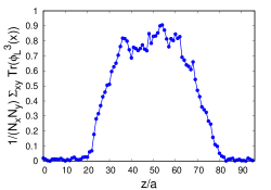
(a) $\frac{1}{N_{x}N_{y}}\sum_{x,y}\mathrm{Tr}\,\left(\Phi_{\mathrm{L}}^{3}({\boldsymbol{x}})\right)$

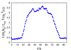
(b) $\frac{1}{N_{x}N_{y}}\sum_{x,y}\mathrm{Tr}\,\left(\Phi_{\mathrm{L}}^{2}({\boldsymbol{x}})\right)$

Figure 1: $\mathrm{Tr}\,\Phi^{3}$ and $\mathrm{Tr}\,\Phi^{2}$, integrated over transverse directions, as a function of the $z$ direction in a $36^{3}\times 96$ box at $g_{3\mathrm{d}}^{2}a=\frac{1}{3}$, $x=0.08896$ and $y=0.47232$. There is a region near 0 (periodically identified with 96) which is in the symmetric phase, and a region near 50 which is in the broken phase, as well as two phase boundaries. The phases are visible in either order parameter but the fluctuations in $\mathrm{Tr}\,\Phi^{2}$ are smaller.

The true order parameter of EQCD is $\mathrm{Tr}\,\Phi^{3}$, which indicates whether the $\mathbb{Z}_{3}$-symmetry of $\Phi$ is present or broken. However, the phase transition can also be spotted in $\mathrm{Tr}\,\Phi^{2}$ (see Fig. 1), which has smaller fluctuations and leads to a more stable phase discriminator; so we use it in the following. Our approach begins by bounding $y_{\mathrm{crit}}$ by performing a simulation in a modest-sized cubic box, starting from a quite positive $y$ value and decreasing it after each update sweep. At some value, $\mathrm{Tr}\,\Phi^{2}$ abruptly jumps. Then one steadily increases $y$ until the value abruptly falls. This determines upper and lower spinodal $y$-values; $y_{\mathrm{crit}}$ must lie between, typically close to the upper value.

Next we estimate $\mathrm{Tr}\,\Phi^{2}_{\mathrm{symm}}$ and $\mathrm{Tr}\,\Phi^{2}_{\mathrm{brok}}$, the values of $\mathrm{Tr}\,\Phi^{2}_{\mathrm{L}}$ in each of these phases at a mass close to the transition temperature, which we do in separate simulations which are initialized with either vanishing or large constant $\Phi$ values. The method will be rather insensitive to the exact values of these quantities, so it is not important if the determinations are from somewhat incorrect $y$ values.

Next we set up our mass tuning algorithm. We work in a rectangular periodic lattice with one long ($L_{z}$) direction and two equal shorter ($L_{x}=L_{y}$) directions. Initially we make the $y$ (Lagrangian) value $z$-coordinate dependent,

$$y(z)=y_{\mathrm{crit,est}}+\Delta y\cos(2\pi z/L_{z})\,,$$ (8)

with $\Delta y$ chosen initially to be large enough that $y_{\mathrm{crit,est}}\pm\Delta y$ are above/below the spinodal values. After a series of update sweeps, the field will find the symmetric phase where $y$ is large and the broken phase where $y$ is small, generating our configuration with both phases and two phase boundaries. Then the magnitude of $\Delta y$ is gradually lowered over a series of update sweeps; if one phase starts to win out over the other, the estimated critical value is adjusted.

With our starting two-phase configuration and estimated $y_{\mathrm{crit}}$ in hand, we proceed to the more accurate determination of $y_{\mathrm{crit}}$. We continue to evolve with a space-uniform $y$ value, but we adjust it after each lattice site-update according to

$$y_{\mathrm{L,\,new}}=y_{\mathrm{L,\,old}}+c_{\mathrm{B}}\cdot\left(\frac{\tfrac{1}{V}\sum_{\boldsymbol{x}}\mathrm{Tr}\,\Phi^{2}-\mathrm{Tr}\,\Phi^{2}_{\mathrm{symm}}}{\mathrm{Tr}\,\Phi^{2}_{\mathrm{brok}}-\mathrm{Tr}\,\Phi^{2}_{\mathrm{symm}}}-0.5\right)\,,$$ (9)

where $y_{L}\equiv Z_{3}(y+\delta y_{2\mathrm{loop}})$ and $c_{\mathrm{B}}$ is a small coefficient that controls the strength of the adjustment. The quantity in brackets here is an estimate for the fraction of the volume which lies in the broken phase, based on the known (approximate) values of $\mathrm{Tr}\,\Phi^{2}$ in each phase. Therefore, the adjustment term shifts $y$ upwards (making the symmetric phase more preferred) when more volume is in the broken phase, and downwards (making the broken phase more preferred) if more of the volume is symmetric.

The coefficient $c_{\mathrm{B}}$ is small, $\mathcal{O}\left(\frac{1}{N_{\mathrm{x}}N_{\mathrm{y}}N_{\mathrm{z}}}\right)$, such that the evolution of $y$ is as mild as possible, consistent with enough restorative force to prevent either phase from “winning.” Specifically, whenever $y$ deviates from $y_{\mathrm{crit}}$, there is a net force on the interface, equal to the surface area times $\Delta F$ the free energy difference between phases. At $y=y_{\mathrm{crit}}$, $\Delta F=0$ and there is no net force on the interface. Away from $y=y_{\mathrm{crit}}$, we can expand $\Delta F$ in a Taylor series in $y-y_{\mathrm{crit}}$. At leading order in small $y-y_{\mathrm{crit}}$, the free energy difference will be linear in $y-y_{\mathrm{crit}}$, and the central value of $y$ which maintains coexistence will equal $y_{\mathrm{crit}}$. At quadratic order, $d^{2}F/dy^{2}\neq 0$ means that the restorative force is slightly biased, and we will obtain an incorrect value for $y_{\mathrm{crit}}$. We test for such a distortion by performing a second evolution where $c_{\mathrm{B}}$ is twice as large, to confirm that the central value of $y$ is the same within errors (which it is in all cases we considered).

4 Results

We use the procedure described in the previous section to determine the critical value $y_{\mathrm{crit}}(x,a)$ for several values of the scalar self-coupling $x$, each at several lattice spacings. The exact list of lattices considered is given in Table 5. Because our procedure leads to relatively long autocorrelation in the estimated $y_{\mathrm{crit}}$ value, the errors must be determined via the jackknife method using relatively wide jackknife bins; we vary the bin widths until the error estimates stabilize. We then subtract the known 1- and 2-loop contributions and apply the known multiplicative rescalings Moore:1997np from the results and convert $y_{\mathrm{L,\,crit}}\rightarrow y_{2\mathrm{loop},\,\mathrm{crit}}$. For each $x$ value, we must extrapolate this quantity to zero lattice spacing; the intercept is the continuum critical $y$ value and the slope at the intercept is the desired $\mathcal{O}(a)$ additive correction to the scalar mass.

Because our $y_{\mathrm{crit}}(x,a)$ results are quite precise but the $a$ values are not extremely small, we anticipate that $y_{\mathrm{crit}}(x,a)$ contains corrections beyond linear order in $a$. In principle, we could straightforwardly fit a polynomial of order $N_{\mathrm{poly}}$ in $g_{3\mathrm{d}}^{2}a$ as

$$y_{\mathrm{crit}}\left(g_{3\mathrm{d}}^{2}a\right)=\sum_{j=0}^{N_{\mathrm{poly}}}\,y_{j}(g_{3\mathrm{d}}^{2}a)^{j}\,.$$ (10)

However, as often occurs, ever-higher order coefficients are ever less certain, and including too many coefficients tends to overfit the data and artificially inflates the final fitting errors. In order to extract these coefficients as efficiently as possible from the data, we would like to build in our knowledge about the convergence of the perturbative series to the fit. A useful tool to implement this is constrained curve fitting Davies:1994mp ; Lepage:2001ym . Motivated by a rough estimate of the radius of convergence $(g_{3\mathrm{d}}^{2}a)_{\mathrm{conv}}\approx 0.5$, we make the a priori-guess

$$|y_{i}|\leq\frac{y_{0}}{2^{i}}\,,$$ (11)

having obtained $y_{0}$ from a standard, unconstrained fit. We then use this estimate to choose the size of a zero-centered chisquare prior on each fitting parameter. The procedure has almost no impact on the determined values of $y_{0}$ and $y_{1}$, where the data is far more constraining than the prior. In practice, a quadratic polynomial is sufficient to give a good fit with a reasonable $\chi^{2}$. The results of these fits are given in Table 2 and the fits themselves are displayed in Fig. 2. We also confirmed by varying the volume that any finite-volume effects are smaller than our statistical error bars.

$x$	$y_{\mathrm{crit,\,cont}}$	$\delta y_{3\mathrm{loop}}/g_{3\mathrm{d}}^{2}a$
$0.0463596$	$0.9293(13)$	$-0.467(19)$
$0.0677528$	$0.67627(85)$	$-0.298(10)$
$0.08896$	$0.54092(76)$	$-0.1750(74)$
$0.13$	$0.4043(18)$	$-0.037(18)$
$0.2$	$0.2961(15)$	$0.004(15)$

Table 2: Results of our five EQCD simulation sets.

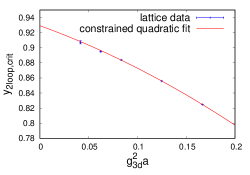
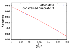
(a) $x=0.0463597$	(b) $x=0.0677528$
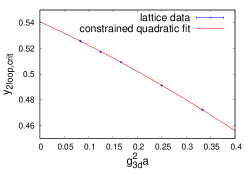
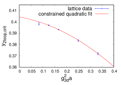
(c) $x=0.08896$	(d) $x=0.13$
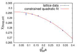
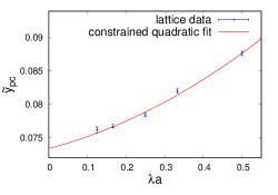
(e) $x=0.2$	(f) pure scalar

Figure 2: Fits of $\mathcal{O}(g_{3\mathrm{d}}^{2}a)$ behavior for different $x$.

We caution the reader that, while $y_{0}$ and $y_{1}$ can be interpreted as the continuum critical point and the 3-loop $\mathcal{O}(a)$ additive mass renormalization coefficient, we cannot interpret $y_{2}$ as a 4-loop mass renormalization or use it to further improve the lattice-continuum matching. That is because there are many uncontrolled $\mathcal{O}(a^{2})$ corrections which influence $y_{2}$. For instance, there are unknown 2-loop $\mathcal{O}(a^{2})$ lattice-continuum corrections to $x$, which influence the critical value via $(dy_{\mathrm{crit}}/dx)\delta x$. Similarly, tree-level $\mathcal{O}(a^{2})$ high-dimension operators and $\mathcal{O}(a^{2})$ corrections to $g^{2}$ (which we could interpret as uncertainties in the scale setting) also lead to $\mathcal{O}(a^{2})$ effects in the $y_{\mathrm{crit}}$ value. Because $(dy_{\mathrm{crit}}/dx)\sim x^{-2}$, the $\mathcal{O}(a^{2})$ and other higher-order effects will become severe as we go towards small $x$ values. Therefore small $x$ requires the use of very fine lattices. Furthermore, when $x$ is small, there becomes a hierarchy of mass scales in the problem; $m_{A,\mathrm{brok}}\gg m_{\Phi}\gg m_{A,\mathrm{symm}}$. Both effects make the accurate extraction of $y_{1}$ at small $x$ very numerically demanding. Therefore we did not treat the smallest $x$ value shown in Table 1. Instead, we add two larger values of $x$, $x=0.13$ and $x=0.20$, which are still within the domain where the transition is first order, but which give us a broader $x$ range over which to fit $y_{1}$ as a function of $x$.

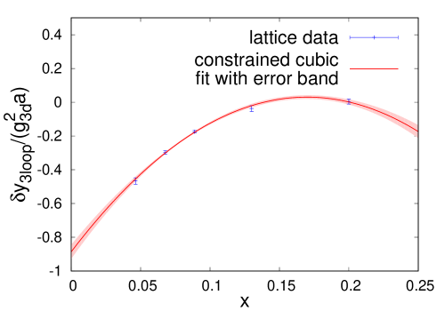
Figure 3: Grand fit of $\frac{\delta y_{\mathrm{3loop}}}{g_{3\mathrm{d}}^{2}a}(x)$ with error band.

Next we use our results for $y_{1}(x)$ to fit its overall $x$ dependence. The parametric form of the $\mathcal{O}(g_{3\mathrm{d}}^{2}a)$-correction DOnofrio:2014mld was given in (7). The $x^{3}$ coefficient corresponds to 3-loop diagrams containing only scalar lines. It is therefore equal to the $\mathcal{O}(a)$ mass renormalization term in the theory in the $g_{3\mathrm{d}}^{2}\to 0$ limit, which is a scalar theory. We explain our (different) procedure to treat this scalar theory in App. A; our analysis leads to the result

$$C_{3}=\frac{\delta\tilde{y}_{\mathrm{3loop}}}{\lambda a}=0.0151(55)\,.$$ (12)

Here $\tilde{y}\equiv m^{2}(\mu=\lambda)/\lambda^{2}$ is the scalar mass, made dimensionless using the scale $\lambda$ rather than the scale $g_{3\mathrm{d}}^{2}$; it equals $y/x^{2}$ up to the effect of the different renormalization scale. We incorporate this result as a prior in fitting a cubic polynomial to the results of Table 2. The resulting fit,

$$\frac{\delta y_{3\mathrm{loop}}}{g_{3\mathrm{d}}^{2}a}(x)=0.0151(55)\,x^{3}-31.8(28)\,x^{2}+10.80(74)\,x-0.886(41)\,,$$ (13)

is displayed in Fig. 3. We report the full error covariance matrix in Table 3. This fit constitutes our main result.

$\mathrm{cov}(C_{i},C_{j})$	$C_{0}$	$C_{1}$	$C_{2}$	$C_{3}$
$C_{0}$	$0.001700$	$-0.02997$	$0.1101$	$-3.563\cdot 10^{-8}$
$C_{1}$	$-0.02997$	$0.5451$	$-2.046$	$1.129\cdot 10^{-6}$
$C_{2}$	$0.1101$	$-2.046$	$7.899$	$-1.079\cdot 10^{-5}$
$C_{3}$	$-3.563\cdot 10^{-8}$	$1.129\cdot 10^{-6}$	$-1.079\cdot 10^{-5}$	$3.025\cdot 10^{-5}$

Table 3: Covariance matrix of the grand fit.

As a corollary, we provide an updated version of the EQCD phase diagram. The version from Kajantie:1998yc does not include continuum-extrapolated critical masses. The intercept of our EQCD fits delivers these critical masses. Additionally, the $x\rightarrow 0$ limit

$$xy_{\mathrm{crit}}=\frac{3}{8\pi^{2}}$$ (14)

is known perturbatively Kajantie:1998yc . We present our data, and this limiting value, in Fig. 4. In addition, to guide the eye, we include a cubic fit of $xy_{\mathrm{crit}}$ as a function of $x$, displayed by a dashed line. There is quantitative agreement with the phase diagram in Kajantie:1998yc at small $x$, but at large $x$ we find that the prominent bending down of the $xy_{\mathrm{crit}}$ curve found by Kajantie:1998yc arose because they failed to take a continuum limit.

Kajantie et al Kajantie:1998yc found that the tricritical point occurs at $x=0.25$, beyond which the phase transition becomes of second order. We have not studied $x$ values larger than $x=0.2$, so we cannot make any statement about the location of the tricritical point.

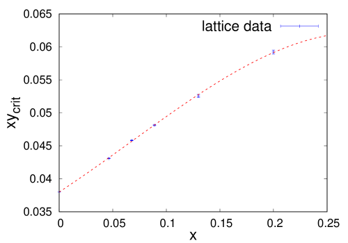
Figure 4: Updated version of the phase diagram of EQCD. The phase below the data points is the $\mathbb{Z}_{3}$-broken phase, the one above is $\mathbb{Z}_{3}$-symmetric. The dashed line is a fit to the datapoints, to help guide the eye.

As a byproduct our study also produces values for the discontinuity in $\mathrm{Tr}\,\Phi^{2}$ across the phase transition point, and for the $\mathcal{O}(a)$ additive correction to the $\mathrm{Tr}\,\Phi^{2}$ operator, which was also not previously known. We postpone these secondary results to Appendix B.

5 Conclusion and outlook

We have computed the remaining $\mathcal{O}(a)$ improvement coefficient in the lattice-continuum matching of 3D EQCD (SU(3) gauge theory with an adjoint scalar in 3 space dimensions). We did so by using the first order phase transition point as a fixed physical point. We developed a new methodology to efficiently extract the critical scalar mass where the first order transition occurs. Determining the critical scalar mass $y_{\mathrm{crit}}(x,a)$ as a function of $a$ for fixed $x$ allows an extrapolation to the continuum limit; the linear term in the extrapolation is the desired improvement coefficient. We then performed a grand fit to its known functional form. As a byproduct, a continuum-extrapolated update of the EQCD phase diagram was obtained.

Now that we are in possession of the last missing ingredient, we aim to compute the modified EQCD-Wilson-loop that leads to $C(q_{\perp})$ and extrapolate it to continuum. The continuum extrapolation is drastically facilitated by our completion of the renormalization Panero:2013pla . The jet broadening coefficient $\hat{q}$ can be derived as the second moment of $C(q_{\perp})$. We hope that the resulting nonperturbative information on $C(q_{\perp})$ will be of utility in studying and interpreting jet modification arising from the hot QCD medium in relativistic heavy ion collisions.

Appendix A Algorithm for pure scalar case

The large-$x$ limit of EQCD is the same as the $g_{3\mathrm{d}}^{2}\to 0$ limit (provided we work in terms of $\tilde{y}\equiv y/x^{2}=m^{2}/\lambda^{2}$ and track the lattice spacing in terms of $\lambda a=g_{3\mathrm{d}}^{2}a\,x$). In this limit, we have an 8 (real) component scalar theory with an $\mathcal{O}(8)$ symmetry and a second-order phase transition where this symmetry is spontaneously broken to $\mathcal{O}(7)$. The $x^{3}$ term in the scalar mass renormalization of EQCD arises purely from scalar diagrams which are identical to those in this theory; therefore we can determine this coefficient by studying the $\mathcal{O}(\lambda a)$ corrections to $\tilde{y}$ in this scalar field theory.

A natural approach would be to use, as a line of constant physics, the 2’nd order phase transition point. However this would face the usual problems of critical slowing down and the inaccuracy of establishing the exact transition point. So we choose instead to compare $\tilde{y}$ between different lattice spacings by finding the pseudocritical value where the theory in a specific physical volume encounters a specific pseudocritical criterion. We choose the volume to be $\lambda L=8$ and select as the pseudocritical condition that the 4th order Binder cumulant Binder:1981sa

$$\mathcal{B}\equiv\frac{\langle\left(\mathrm{Tr}\,\bar{\Phi}^{2}\right)^{2}\rangle}{\langle\mathrm{Tr}\,\bar{\Phi}^{2}\rangle^{2}}\,,$$ (15)

where $\bar{\Phi}\equiv\tfrac{1}{N^{3}}\sum_{\boldsymbol{x}}\Phi_{\mathrm{L}}({\boldsymbol{x}})$, takes the value $\mathcal{B}_{\mathrm{pc}}=1.073$. Because the Binder cumulant is dominated by infrared physics and is insensitive to the lattice spacing up to subleading corrections and renormalization effects (which are what we want to study), this should occur at the same physical $y$ value at every lattice spacing up to $\mathcal{O}(a^{2})$ or higher corrections. Our set of simulation parameters can be found in Table 4. The results already appeared in the last panel of Fig. 2.

$\lambda a$	$N_{\mathrm{x}}N_{\mathrm{y}}N_{\mathrm{z}}$	total statistics
$1/2$	$16^{3}$	$402900$
$1/3$	$24^{3}$	$1490120$
$1/4$	$32^{3}$	$2487440$
$1/6$	$48^{3}$	$2931750$
$1/8$	$64^{3}$	$2513280$

Table 4: Simulation parameters for the pure scalar simulation.

Appendix B EQCD simulation parameters and phase transition properties

B.1 Parameters and table

In Table 5, we provide parameters and direct results of our EQCD simulations as well as values for $\mathrm{Tr}\,\Phi^{2}$ in both phases at criticality. We converted $\mathrm{Tr}\,\Phi^{2}_{\mathrm{L,crit}}\rightarrow\frac{\mathrm{Tr}\,\Phi^{2}_{\mathrm{crit,cont}}}{g_{3\mathrm{d}}^{2}}$, where we display the latter in the table, via all known contributions up to $\mathcal{O}(g_{3\mathrm{d}}^{2}a)$ in Eq. (18) Moore:1997np . For the sake of readability, we will refer to $\frac{\mathrm{Tr}\,\Phi^{2}_{\mathrm{crit,cont}}}{g_{3\mathrm{d}}^{2}}$ as $\frac{\mathrm{Tr}\,\Phi^{2}}{g_{3\mathrm{d}}^{2}}$ in the following. The raw data was obtained in separate simulations with $V=N_{\mathrm{x}}^{3}$. We ensured that the Monte-Carlo error of the separate simulations dominates the overall error of $\frac{\mathrm{Tr}\,\Phi^{2}}{g_{3\mathrm{d}}^{2}}$, not the uncertainty of $y_{\mathrm{crit}}$. The slightly negative values of $\frac{\mathrm{Tr}\,\Phi^{2}_{\mathrm{symm}}}{g_{3\mathrm{d}}^{2}}$ for small $x$ are expected and arise because the positive mass-squared at the transition point suppresses IR fluctuations, while the renormalization involves subtracting off large positive counterterms (including the massless, free-theory fluctuations).

$g_{3\mathrm{d}}^{2}a$	$x_{\mathrm{cont}}$	$N_{\mathrm{x}}N_{\mathrm{y}}N_{\mathrm{z}}$	$y_{\mathrm{crit,cont}}$	statistics $y_{\mathrm{crit}}$	​$\mathrm{Tr}\,\Phi^{2}_{\mathrm{brok}}/g_{3\mathrm{d}}^{2}\!$	$\mathrm{Tr}\,\Phi^{2}_{\mathrm{symm}}/g_{3\mathrm{d}}^{2}$
$1/6$	$0.0463597$	$72^{2}\times 192$	$0.824773(45)$	$300690$	$14.0477(40)$	$-0.22234(28)$
$1/8$	$0.0463597$	$96^{2}\times 256$	$0.855935(85)$	$373030$	$15.4237(89)$	$-0.23064(43)$
$1/12$	$0.0463597$	$144^{2}\times 384$	$0.88387(28)$	$37170$	$17.716(12)$	$-0.23390(77)$
$1/16$	$0.0463597$	$192^{2}\times 512$	$0.89504(62)$	$1300$	$17.714(14)$	$-0.23748(74)$
$1/24$	$0.0463597$	$192^{2}\times 512$	$0.9072(21)$	$1430$	$17.585(57)$	$-0.2355(17)$
$1/4$	$0.0677528$	$48^{2}\times 128$	$0.59100(19)$	$13110$	$6.7502(59)$	$-0.11392(62)$
$1/6$	$0.0677528$	$72^{2}\times 192$	$0.62149(12)$	$150000$	$7.6155(72)$	$-0.12043(55)$
$1/8$	$0.0677528$	$96^{2}\times 256$	$0.63661(11)$	$200000$	$7.960(14)$	$-0.12101(78)$
$1/12$	$0.0677528$	$144^{2}\times 384$	$0.64963(29)$	$38990$	$8.287(15)$	$-0.12400(80)$
$1/16$	$0.0677528$	$192^{2}\times 512$	$0.6546(11)$	$1910$	$8.4103(61)$	$-0.1228(12)$
$1/3$	$0.08896$	$36^{2}\times 96$	$0.47232(24)$	$10000$	$4.0728(22)$	$-0.03277(47)$
$1/4$	$0.08896$	$48^{2}\times 128$	$0.49119(14)$	$100000$	$4.4343(53)$	$-0.03489(59)$
$1/6$	$0.08896$	$72^{2}\times 192$	$0.50940(15)$	$150000$	$4.7728(35)$	$-0.0344(10)$
$1/8$	$0.08896$	$96^{2}\times 256$	$0.51736(20)$	$97500$	$4.9249(58)$	$-0.0336(11)$
$1/12$	$0.08896$	$144^{2}\times 384$	$0.52565(45)$	$44530$	$5.052(10)$	$-0.0321(13)$
$1/3$	$0.13$	$36^{2}\times 96$	$0.37184(94)$	$10000$	$2.3337(64)$	$0.1112(15)$
$1/4$	$0.13$	$48^{2}\times 128$	$0.38341(83)$	$100000$	$2.3899(64)$	$0.1126(19)$
$1/6$	$0.13$	$72^{2}\times 192$	$0.39323(21)$	$150000$	$2.4703(75)$	$0.1190(38)$
$1/8$	$0.13$	$96^{2}\times 256$	$0.39702(31)$	$109230$	$2.5371(82)$	$0.1246(39)$
$1/12$	$0.13$	$144^{2}\times 384$	$0.3982(11)$	$120600$	$2.618(13)$	$0.1332(65)$
$1/3$	$0.2$	$36^{2}\times 96$	$0.27743(41)$	$12340$	$1.3115(74)$	$0.578(32)$
$1/4$	$0.2$	$48^{2}\times 128$	$0.28595(34)$	$21030$	$1.283(13)$	$0.630(34)$
$1/6$	$0.2$	$72^{2}\times 192$	$0.29214(37)$	$66160$	$1.2850(81)$	$0.650(24)$
$1/8$	$0.2$	$96^{2}\times 256$	$0.29377(48)$	$122080$	$1.323(11)$	$0.713(37)$
$1/12$	$0.2$	$144^{2}\times 384$	$0.29393(97)$	$3330$	$1.390(14)$	$0.707(26)$

Table 5: Parameters and results of EQCD simulations.

B.2 Transition strength

With the critical values of $\frac{\mathrm{Tr}\,\Phi^{2}}{g_{3\mathrm{d}}^{2}}$ in both phases from Table 5 in hand, we can infer further interesting features of the first order phase transition. Having several values of $\frac{\mathrm{Tr}\,\Phi^{2}}{g_{3\mathrm{d}}^{2}}$ at the same physical $x$ and different lattice spacings $g_{3\mathrm{d}}^{2}a$, we extrapolate both the difference between phases $\frac{\Delta\mathrm{Tr}\,\Phi^{2}}{g_{3\mathrm{d}}^{2}}$ and the symmetric phase value $\frac{\mathrm{Tr}\,\Phi^{2}_{\mathrm{symm}}}{g_{3\mathrm{d}}^{2}}$ to the continuum. We provide the former in Fig. 5 and the latter in Fig. 6. The continuum limits, and the linear coefficient in the fit for the case of $\frac{\mathrm{Tr}\,\Phi^{2}_{\mathrm{symm}}}{g_{3\mathrm{d}}^{2}}$, are provided in Table 6.

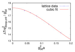
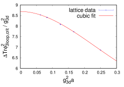
(a) $x=0.0463597$	(b) $x=0.0677528$
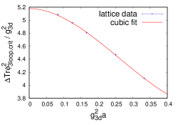
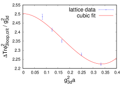
(c) $x=0.08896$	(d) $x=0.13$
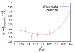
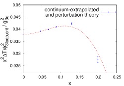
(e) $x=0.2$	(f) $\frac{\Delta\mathrm{Tr}\,\Phi^{2}}{g_{3\mathrm{d}}^{2}}(x)$

Figure 5: Continuum extrapolation of $\frac{\Delta\mathrm{Tr}\,\Phi^{2}}{g_{3\mathrm{d}}^{2}}$, the difference of the broken and symmetric phase value of $\frac{\mathrm{Tr}\,\Phi^{2}}{g_{3\mathrm{d}}^{2}}$, at different $x$. The intercept in (f) was determined analytically in Kajantie:1998yc and was incorporated into that plot.

$x$	$\mathrm{Tr}\,\Phi^{2}_{\mathrm{symm,cont}}/g_{3\mathrm{d}}^{2}$	$\delta\mathrm{Tr}\,\Phi^{2}_{\mathrm{3loop}}/g_{3\mathrm{d}}^{4}a$	$\Delta\mathrm{Tr}\,\Phi^{2}_{\mathrm{cont}}/g_{3\mathrm{d}}^{2}$
$0.0463597$	$-0.2350(24)$	$-0.081(44)$	$18.232(27)$
$0.0677528$	$-0.1231(22)$	$-0.019(30)$	$8.692(13)$
$0.08896$	$-0.0272(27)$	$-0.072(25)$	$5.177(11)$
$0.13$	$0.151(11)$	$-0.256(70)$	$2.502(24)$
$0.2$	$0.763(76)$	$-0.66(85)$	$0.689(33)$

Table 6: Continuum-extrapolated $\frac{\mathrm{Tr}\,\Phi^{2}}{g_{3\mathrm{d}}^{2}}$ in the symmetric phase at criticality, $\mathcal{O}(a)$ operator improvement of $\frac{\mathrm{Tr}\,\Phi^{2}}{g_{3\mathrm{d}}^{2}}$ and continuum- extrapolated difference of $\frac{\mathrm{Tr}\,\Phi^{2}}{g_{3\mathrm{d}}^{2}}$ in the two phases at criticality.

The limiting values of the fits provide us with two interesting pieces of information about the phase transition in this theory. The most interesting is $\frac{\Delta\mathrm{Tr}\,\Phi^{2}}{g_{3\mathrm{d}}^{2}}$, which measures the strength of the phase transition. For small $x$ we can predict this strength perturbatively; the limiting behavior is Kajantie:1998yc $\frac{\Delta\mathrm{Tr}\,\Phi^{2}}{g_{3\mathrm{d}}^{2}}=3/(8\pi^{2}x^{2})$, which we also include in the last frame of Fig. 5. We have provided a cubic fit to guide the eye, but it should not be taken seriously; the strength of the phase transition is a nonperturbative quantity and there is no reason to expect it to take such a simple form. In fact, we know that $\frac{\Delta\mathrm{Tr}\,\Phi^{2}}{g_{3\mathrm{d}}^{2}}\to 0$ as $x\to x_{\mathrm{triple}}$, with a nontrivial critical exponent. Note that in the fit for the $a$ dependence of $\frac{\Delta\mathrm{Tr}\,\Phi^{2}}{g_{3\mathrm{d}}^{2}}$, we have fitted to a polynomial without a linear term; this is because the known $\mathcal{O}(a)$ corrections are sufficient to eliminate such a linear correction in the difference between phases of $\frac{\mathrm{Tr}\,\Phi^{2}}{g_{3\mathrm{d}}^{2}}$.

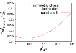
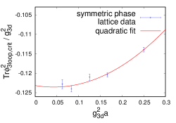
(a) $x=0.0463597$	(b) $x=0.0677528$
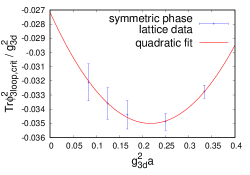
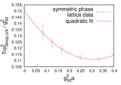
(c) $x=0.08896$	(d) $x=0.13$
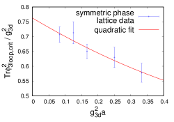
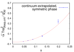
(e) $x=0.2$	(f) Function-of-$x$
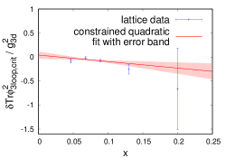
(g) Grand fit $\frac{\delta\mathrm{Tr}\,\Phi^{2}_{\mathrm{3loop}}}{g_{3\mathrm{d}}^{4}a}(x)$

Figure 6: Fits of $\frac{\mathrm{Tr}\,\Phi^{2}}{g_{3\mathrm{d}}^{2}}(g_{3\mathrm{d}}^{2}a)$ at different $x$ and grand fit.

B.3 Additive operator improvement

On the other hand, the value of either $\frac{\mathrm{Tr}\,\Phi^{2}_{\mathrm{symm}}}{g_{3\mathrm{d}}^{2}}$ or $\frac{\mathrm{Tr}\,\Phi^{2}_{\mathrm{brok}}}{g_{3\mathrm{d}}^{2}}$, by themselves, still contain $\mathcal{O}(a)$ errors, since there is an unknown additive renormalization to the operator $\mathrm{Tr}\,\Phi^{2}$ which arises at 3 loops. Since the correction is additive and both phases were explored at the same $y$ value, these effects cancel in the difference. We took advantage of this cancellation in the last subsection. But now our goal is to use this linear behavior to extract the unknown $\mathcal{O}(a)$ additive corrections to the $\Phi^{2}$ operator. These arise at 3 loops in a perturbative lattice-continuum matching calculation, which is prohibitive; so we will again try to extract them from the data.

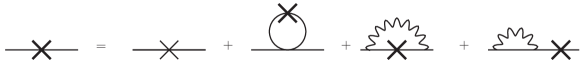
Figure 7: Diagrams generating $Z_{m}$ the multiplicative $\mathrm{Tr}\>\Phi^{2}$ operator renormalization. Heavy crosses are the renormalized operator (with $Z_{m}$ factor), while light crosses are the bare operator.

Because we are working to 3 loops, we must specify quite carefully how 1-loop multiplicative effects will be implemented, since they can multiply one and two loop additive effects to give 3-loop level contributions, which then differ depending on our exact procedure. Here we will depart slightly from the procedure of Refs Moore:1997np ; Arnold:2001ir ; DOnofrio:2014mld . We write the continuum expectation value as

$$\frac{\mathrm{Tr}\,\Phi^{2}_{\mathrm{cont}}}{g_{3\mathrm{d}}^{2}}=Z_{m}\left(Z_{\Phi}\mathrm{Tr}\,\Phi^{2}_{\mathrm{L}}-\frac{\delta\Phi^{2}}{g_{3\mathrm{d}}^{2}}\right)\,,$$ (16)

where $Z_{m}$ is the 1-loop multiplicative renormalization factor of the $\mathrm{Tr}\,\Phi^{2}$ operator, and $Z_{\Phi}$ accounts for our choice of scalar field normalization on the lattice (see Eq. (3)). Examining the 3-loop diagrams, we find that certain 3-loop effects are absorbed if we define $Z_{m}$, resumming the Dyson series. That is, in Figure 7, we take the operator inserted on the 1-loop diagrams to be the resummed, rather than the bare, operator, which will sum the Dyson series, leading to an expression for $Z_{m}^{-1}$. Slightly rearranging Eq.(32,33) of Ref. Moore:1997np , we find

$$Z_{m}^{-1}=1+\frac{g_{3\mathrm{d}}^{2}a}{4\pi}\left(3N\xi+\frac{N\Sigma}{6}-(N^{2}+1)\xi x\right)\,.$$ (17)

Here $\xi=0.152859324966$ and $\Sigma=3.17591153562522$ are standard integrals encountered in the 1-loop lattice-continuum matching. We are also writing the number of colors $N=3$ explicitly, to show the detailed dependence on the number of colors. With this definition, the two-loop and partially 3-loop result for $\delta\Phi^{2}$ is

$$\frac{\delta\Phi^{2}}{g_{3\mathrm{d}}^{2}} = \frac{N^{2}-1}{2g_{3\mathrm{d}}^{2}a}\left[\frac{\Sigma}{4\pi}-\frac{\xi yg_{3\mathrm{d}}^{4}a^{2}}{4\pi}+\frac{Ng_{3\mathrm{d}}^{2}a}{(4\pi)^{2}}Z_{m}^{-1}\left(2\ln\frac{6}{g_{3\mathrm{d}}^{2}a}+2\zeta-2\delta+\frac{\Sigma^{2}}{2}\right)\right.$$ (18)

$$\phantom{\frac{N^{2}-1}{2g_{3\mathrm{d}}^{2}a}}\left.{}+\frac{g_{3\mathrm{d}}^{4}a^{2}}{(4\pi)^{3}}\Big{(}2\xi(N^{2}+1)(x^{2}-Nx)\ln(g_{3\mathrm{d}}^{2}a)+C_{\Phi a}+C_{\Phi b}x+C_{\Phi c}x^{2}\Big{)}\right].\quad$$

The unknown coefficients $C_{\Phi a}$, $C_{\Phi b}$ and $C_{\Phi c}$ capture the remaining $\mathcal{O}(a)$ corrections from 3-loop diagrams which are not iterations of simpler 1 and 2 loop diagrams. Note that Eq. (18) contains several terms proportional to $\ln(g_{3\mathrm{d}}^{2}a)$. These arise from logarithmic divergences in the continuum theory, regulated at our choice of renormalization point $\mu=g_{3\mathrm{d}}^{2}$ but then cut off on the lattice at the scale $1/a$. The term next to $\zeta-\delta$ is the explicit $\mu^{2}$ dependence of $\Phi^{2}/g_{3\mathrm{d}}^{2}$ and is therefore expected; the coefficient $Z_{m}^{-1}$ ensures that it enters Eq. (16) with precisely the right continuum normalization. The log terms proportional to $\xi$ in the last line cancel the $\mu$ dependence of the mass squared ($y$) in the mass-dependent $\mathcal{O}(a)$ shift in the first line.

It remains to determine the three coefficients in the last line. In fact, we only need to fit two of these coefficients; one of them, $C_{\Phi c}$, represents pure-scalar corrections, which can be extracted from Ref. Arnold:2001ir . The reference performs the calculation for an improved hopping term, but repeating the calculation for the nearest-neighbor hopping term we use here, we find that

$$C_{\Phi c}=2(N^{2}+1)C_{4}\,,\qquad C_{4}=0.5630(4)\,,$$ (19)

which differs from the result in the reference, $C_{4,\mathrm{Ref}}=0.2817$, because of the different scalar dispersion between the nearest-neighbor hopping term used here and the improved hopping term used there.

After performing these subtractions, we can fit the residual linear $a$-dependence of $\mathrm{Tr}\,\Phi^{2}_{\mathrm{L}}$ for each $x$ value we consider, and extract the coefficients $C_{\Phi a},C_{\Phi b}$ from a grand fit in complete analogy with the $m^{2}$ effects we consider in the main text. We find

$$C_{\Phi a} =(-21\pm 37)$$ (20)

$$C_{\Phi b} =(6.7\pm 4.7)\times 10^{2}\,,$$ (21)

again by constrained curve fitting. The grand fit is displayed in the seventh frame of Fig. 6. Unfortunately, it appears that our results fail to constrain these coefficients very much. The full covariance matrix can be found in Tab. 7. From the covariance matrix, we can also see that the error of $C_{\Phi c}$ is by far the smallest, so value and error of $C_{\Phi c}$ were not changed by the constrained fit.

$\mathrm{cov}(C_{i},C_{j})$	$C_{\Phi a}$	$C_{\Phi b}$	$C_{\Phi c}$
$C_{\Phi a}$	$21694$	$-267617$	$5.3859\cdot 10^{-6}$
$C_{\Phi b}$	$-267617$	$3.4914\cdot 10^{6}$	$-1.432\cdot 10^{-4}$
$C_{\Phi c}$	$5.3859\cdot 10^{-6}$	$-1.432\cdot 10^{-4}$	$9.0\cdot 10^{-4}$

Table 7: Covariance matrix of the grand fit of the missing 3 loop $\frac{\delta\Phi^{2}}{g_{3\mathrm{d}}^{2}}$-contribution.

References

- [1] A. Bazavov et al. Equation of state in ( 2+1 )-flavor QCD. Phys. Rev., D90:094503, 2014.
- [2] Szabocls Borsanyi, Zoltan Fodor, Christian Hoelbling, Sandor D. Katz, Stefan Krieg, and Kalman K. Szabo. Full result for the QCD equation of state with 2+1 flavors. Phys. Lett., B730:99–104, 2014.
- [3] Edward V. Shuryak. Theory of Hadronic Plasma. Sov. Phys. JETP, 47:212–219, 1978. [Zh. Eksp. Teor. Fiz.74,408(1978)].
- [4] Joseph I. Kapusta. Quantum Chromodynamics at High Temperature. Nucl. Phys., B148:461–498, 1979.
- [5] T. Toimela. The next term in the thermodynamic potential of qcd. Physics Letters B, 124(5):407 – 409, 1983.
- [6] Peter Brockway Arnold and Cheng-xing Zhai. The Three loop free energy for high temperature QED and QCD with fermions. Phys. Rev., D51:1906–1918, 1995.
- [7] Cheng-xing Zhai and Boris M. Kastening. The Free energy of hot gauge theories with fermions through g**5. Phys. Rev., D52:7232–7246, 1995.
- [8] K. Kajantie, M. Laine, K. Rummukainen, and Y. Schroder. The Pressure of hot QCD up to g6 ln(1/g). Phys. Rev., D67:105008, 2003.
- [9] M. Laine. What is the simplest effective approach to hot QCD thermodynamics? In Proceedings, 5th Internationa Conference on Strong and Electroweak Matter (SEWM 2002): Heidelberg, Germany, October 2-5, 2002, pages 137–146, 2003.
- [10] Andrei D. Linde. Infrared Problem in Thermodynamics of the Yang-Mills Gas. Phys. Lett., 96B:289–292, 1980.
- [11] Eric Braaten and Agustin Nieto. Effective field theory approach to high temperature thermodynamics. Phys. Rev., D51:6990–7006, 1995.
- [12] Thomas Appelquist and Robert D. Pisarski. High-Temperature Yang-Mills Theories and Three-Dimensional Quantum Chromodynamics. Phys. Rev., D23:2305, 1981.
- [13] Sudhir Nadkarni. Dimensional Reduction in Hot QCD. Phys. Rev., D27:917, 1983.
- [14] K. Kajantie, M. Laine, K. Rummukainen, and Mikhail E. Shaposhnikov. 3-D SU(N) + adjoint Higgs theory and finite temperature QCD. Nucl. Phys., B503:357–384, 1997.
- [15] M. Laine and Y. Schroder. Two-loop QCD gauge coupling at high temperatures. JHEP, 03:067, 2005.
- [16] A. Hart, M. Laine, and O. Philipsen. Static correlation lengths in QCD at high temperatures and finite densities. Nucl. Phys., B586:443–474, 2000.
- [17] Ari Hietanen and Kari Rummukainen. The Diagonal and off-diagonal quark number susceptibility of high temperature and finite density QCD. JHEP, 04:078, 2008.
- [18] Simon Caron-Huot. O(g) plasma effects in jet quenching. Phys. Rev., D79:065039, 2009.
- [19] Steffen A. Bass, Charles Gale, Abhijit Majumder, Chiho Nonaka, Guang-You Qin, Thorsten Renk, and Jorg Ruppert. Systematic Comparison of Jet Energy-Loss Schemes in a realistic hydrodynamic medium. Phys. Rev., C79:024901, 2009.
- [20] Jorge Casalderrey-Solana and Derek Teaney. Transverse Momentum Broadening of a Fast Quark in a N=4 Yang Mills Plasma. JHEP, 04:039, 2007.
- [21] Marco Panero, Kari Rummukainen, and Andreas Schäfer. Lattice Study of the Jet Quenching Parameter. Phys. Rev. Lett., 112(16):162001, 2014.
- [22] Guy D. Moore. O(a) errors in 3-D SU(N) Higgs theories. Nucl. Phys., B523:569–593, 1998.
- [23] Michela D’Onofrio, Aleksi Kurkela, and Guy D. Moore. Renormalization of Null Wilson Lines in EQCD. JHEP, 03:125, 2014.
- [24] A. Vuorinen and Laurence G. Yaffe. Z(3)-symmetric effective theory for SU(3) Yang-Mills theory at high temperature. Phys. Rev., D74:025011, 2006.
- [25] K. Farakos, K. Kajantie, M. Laine, K. Rummukainen, and M. Shaposhnikov. Results from 3d electroweak phase transition simulations. Nuclear Physics B - Proceedings Supplements, 47(1):705 – 708, 1996.
- [26] K. Kajantie, M. Laine, K. Rummukainen, and Mikhail E. Shaposhnikov. The Electroweak phase transition: A Nonperturbative analysis. Nucl. Phys., B466:189–258, 1996.
- [27] http://luscher.web.cern.ch/luscher/openQCD/index.html.
- [28] K. Kajantie, M. Laine, A. Rajantie, K. Rummukainen, and M. Tsypin. The Phase diagram of three-dimensional SU(3) + adjoint Higgs theory. JHEP, 11:011, 1998.
- [29] Mattia Bruno, Mattia Dalla Brida, Patrick Fritzsch, Tomasz Korzec, Alberto Ramos, Stefan Schaefer, Hubert Simma, Stefan Sint, and Rainer Sommer. QCD Coupling from a Nonperturbative Determination of the Three-Flavor Parameter. Phys. Rev. Lett., 119(10):102001, 2017.
- [30] C. T. H. Davies, K. Hornbostel, A. Langnau, G. P. Lepage, A. Lidsey, J. Shigemitsu, and J. H. Sloan. Precision Upsilon spectroscopy from nonrelativistic lattice QCD. Phys. Rev., D50:6963–6977, 1994.
- [31] G. P. Lepage, B. Clark, C. T. H. Davies, K. Hornbostel, P. B. Mackenzie, C. Morningstar, and H. Trottier. Constrained curve fitting. Nucl. Phys. Proc. Suppl., 106:12–20, 2002.
- [32] Peter Brockway Arnold and Olivier Espinosa. The Effective potential and first order phase transitions: Beyond leading-order. Phys. Rev., D47:3546, 1993. [Erratum: Phys. Rev.D50,6662(1994)].
- [33] K. Binder. Finite size scaling analysis of Ising model block distribution functions. Z. Phys., B43:119–140, 1981.
- [34] A. Hietanen, K. Kajantie, M. Laine, K. Rummukainen, and Y. Schroder. Three-dimensional physics and the pressure of hot QCD. Phys. Rev., D79:045018, 2009.
- [35] Peter Brockway Arnold and Guy D. Moore. Monte Carlo simulation of O(2) phi**4 field theory in three-dimensions. Phys. Rev., E64:066113, 2001. [Erratum: Phys. Rev.E68,049902(2003)].