Pose estimator and tracker
using temporal flow maps for limbs

Abstract

For human pose estimation in videos, it is significant how to use temporal information between frames. In this paper, we propose temporal flow maps for limbs (TML) and a multi-stride method to estimate and track human poses. The proposed temporal flow maps are unit vectors describing the limbs’ movements. We constructed a network to learn both spatial information and temporal information end-to-end. Spatial information such as joint heatmaps and part affinity fields is regressed in the spatial network part, and the TML is regressed in the temporal network part. We also propose a data augmentation method to learn various types of TML better. The proposed multi-stride method expands the data by randomly selecting two frames within a defined range. We demonstrate that the proposed method efficiently estimates and tracks human poses on the PoseTrack 2017 and 2018 datasets.

I Introduction

Human pose estimation (HPE) is one of the most significant tasks in computer vision. Over the past few years, static image-based pose estimation for either a single person or multiple people has achieved high accuracy using convolutional neural networks (CNNs). Deeply-structured networks as well as iterative networks have been proposed for this task to take advantage of their large receptive fields and rich representation power.

In case of multiple people pose estimation, there are two major approaches: top-down and bottom-up approaches. The bottom-up approach [1, 2, 3, 4, 5, 6, 7, 8, 9, 10] detects the body joints of all people at once and then estimates human poses individually. On the other hand, the top-down approach [11, 12, 13, 5, 14, 15, 16] consists of a human detector that detects human bounding boxes and a single person pose estimator that locates and groups body joints in each bounding box.

Recently, HPE in videos has grabbed attentions as an extension of HPE in a single image. For HPE in videos, human pose tracking should be performed as well as the pose estimation. Many researches have exploited temporal information in various ways for tracking. Such methods as a bounding box tracking algorithm, optical flow, similarity of estimated shape, temporal flow fields (TFF) and so on have been applied for this task [15, 8, 16, 2].

Among them, the work of Xiao et al. [15] is a representative top-down approach. They detected the pose based on the extracted bounding boxes and proposed a box tracking method for pose tracking, which is a combination of a box propagation using optical flow and a flow-based pose similarity. Likewise, Ibrahim et al. [8] used the similarity of the poses to track the pose while it is a bottom-up approach. In case of [16], they proposed an online pose tracking algorithm called pose flow, which is an association of the same person in different frames. They created the optimized pose flow using several scores such as mean score of all keypoints. In summary, these studies proposed tracking methods based on the similarity of estimated poses.

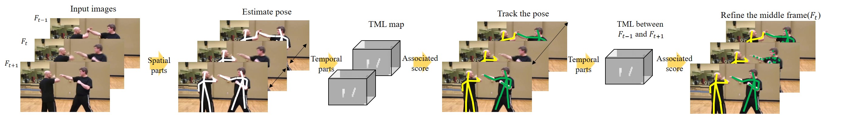
Figure 1: An inference flow of proposed method. A set of frames ($F_{t-1}$, $F_{t}$, $F_{t+1}$) is defined for temporal inference. Two frames that are ($F_{t-1}$, $F_{t}$) or ($F_{t}$, $F_{t+1}$) are input into the network as a pair. First, poses are estimated using the spatial part on the each frame and TML are extracted by the temporal part at the same time. To track poses, we calculate the association score of each person using the TML and the joint distance score. The optimal connection is found by using a bipartite method. In order to refine the middle of frame $F_{t}$, we need to get the associated information between ($F_{t-1}$, $F_{t+1}$) through the TML and the joint distance. If the pose is connected between $F_{t-1}$ and $F_{t+1}$, we added the average pose of between ($F_{t-1}$, $F_{t+1}$). Note that, the time interval of TML is 1 at inference stage but it can be a greater number at training stage which will be described in the multi-stride method.

On the other hand, Andreas et al. [2] represented an association of poses as temporal vector maps called temporal flow fields (TFF). TFF indicates the flow of a joint between two frames. They estimated poses through the heatmaps and part affinity fields [1] and used a similarity measure in a bipartite graph matching to track the poses. However, when estimating TFF, using only joint location may not be enough to track the poses. Tracking only a single joint may lead to a lack of representation power or may be vulnerable to occlusion of joints. Therefore, if a limb that connects two joints is tracked, it is expected to provide richer representation for the tracker and to enhance robustness to occlusion. In addition, considering frames of multiple strides rather than only two consecutive frames can further improve the robustness and performance of the network.

To this end, in this paper, we propose a pose estimator and tracker based on TML which is designed to represent a temporal movement of a person by estimating the direction of limbs’ movement. More specifically, we subdivide each limb into several sections equally in each frame. Then, 2D unit vectors that represent the direction of corresponding limb sections between two frames are calculated, which are used to build each limb’s temporal maps. A huge amount of data is needed to train the TML because the maps have to learn extensive information. Thus, we develop a multi-stride method as a data augmentation method to learn various types of TML. In other words, we randomly take the two frames within a given time range.

Figure 1 shows the overall flow of inference in the proposed method. During inference, we process three frames as a frame set at a time. First, we extract poses on each frame in the form of joint heatmaps and part affinity fields at the spatial part. The extracted poses are tracked between the first and the second frame of the three frames by associated scores obtained from a TML score and a joint distance. The second frame lies in the middle of the consecutive three frames. After the same procedure is applied to the second frame and the third frame, the second frame is refined by analyzing the association scores of the three frames. The frame set is selected at one frame interval. This makes the model stable since the information from the frames back and forth adjust the result of the intermediate frame.

Thus, the contributions of our work are as follows:

1) We propose the TML to represent directions of limbs’ movement.

2) A multi-stride method is proposed to train various TML as a data augmentation method.

3) The current poses are refined by associated score of the previous frame and the next frame.

We evaluated the proposed method on the PoseTrack 2017 and 2018 datasets [17]. To prove the effectiveness of the proposed method, we made a comparison of our work with state-of-the-art algorithms.

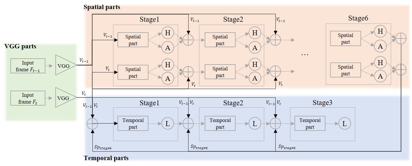
Figure 2: The structure of the proposed network. The spatial and the temporal parts are combined together in a single network. On the spatial part, joint heatmaps (H circle) and part affinity fields (A circle) are regressed. Outputs from the spatial part and features from the final layers of the VGG parts are fed into the temporal part. The temporal part regresses the TML (L circle). Pixel-wise L2 losses are used to optimize all the outputs. $V_{t-1}$ and $V_{t}$ mean the extracted features from VGG parts at $t-1$ and $t$ frame respectively. $Sp_{stage6}$ is the concatenated spatial features of $t-1$ frame and $t$ frame at the stage6.

II Related work

II-A Single person pose estimation

Over the past few years, many CNN based methods in single person pose estimation [18, 19, 20, 3, 21, 7, 22, 23, 24, 25, 26] used very deep networks. Also, a recursive methodology has been adopted in many competitive methods.

Newell et al. [21] proposed a model with multiple hourglass modules that repeats bottom-up and top-down processing and Wei et al. [25] proposed a convolution version of the pose machine [22] which has been proposed by Ramakrishna et al. Features in these networks possess a large receptive field which extracts an efficient representation of human context. Advances in the single person pose estimation have made it possible to proceed research on multi-person pose estimation.

II-B Multi person pose estimation

Multi-person pose estimation [1, 2, 11, 12, 27, 3, 4, 5, 13, 6, 14, 7, 8, 9, 15, 16, 10] methods can be categorized as top-down and bottom-up approaches. The top-down approaches [11, 12, 13, 5, 14, 15, 16] firstly detect a person’s bounding box and estimate single pose on the extracted bounding box. On the other hand, the bottom-up approaches [1, 2, 3, 4, 5, 6, 7, 8, 9, 10] firstly detect parts of people and then determine poses in the input image by connecting the candidate parts.

Cao et al. [1] proposed part affinity fields (PAFs) to associate body parts and determined the pose using the PAFs. Doering et al. [2] and Zhu et al. [10] suggested modified version of methods based on this model. DeeperCut [7] is a graph decomposition method to re-define a variable number of consistent body part configurations. The performances of state-of-the-art multi-person pose estimation methods are pretty good for a single frame. However, to apply the methods on real applications, we need to combine them with tracking algorithms for video data.

II-C Human pose estimation with tracking

Several methods have been proposed to estimate and track human poses on videos [2, 12, 27, 4, 5, 15, 16]. These methods can be divided into two groups depending on whether the learned temporal information is used or not. For the methods that do not use the learned temporal information, they track the pose by applying optical flow, box tracking algorithm, and so on. Xiu et al. [16] proposed a pose tracker based on a pose flow that is a flow structure indicating the same person in different frames by pose distance. Xiao et al. [15] tracked the pose to use a flow-based pose tracking algorithm based on box propagation using optical flow and a flow-based pose similarity. Instead of naively connecting the relationships between detected poses, several papers trained sequential information. Radwan et al. [8] used a bi-directional long-short term memory (LSTM) framework to learn the consistencies of the human body shapes. Doering et al. [2] proposed temporal flow fields that are vector fields to indicate the direction of joints.

However, tracking only a single joint may not contain enough temporal information due to lack of representation power and also it may be vulnerable to occlusion of joints. Therefore, in this paper, instead of a single joint point, a limb connecting two adjacent joints is tracked, which is expected to resolve the above mentioned problems. Also, during both training and testing, we consider a pair of frames with more than one time interval rather than only using two consecutive frames for the robustness of the proposed architecture.

III Method

In order to estimate and track human poses using a single network, we constructed a network consisting of two sub-parts (a spatial part and a temporal part) as shown in Figure 2. We used the network presented in [1] for the spatial part, which has iterative stages. The stage consists of two branches, one for joint heatmaps and the other for part affinity fields. In the proposed network, we take two frames as inputs. Each frame passes through the VGG network to extract features [28]. The features of each frame are fed into each spatial part of the network in parallel. The features of two input frames and the output of the spatial part’s last stage are concatenated and fed into the temporal part. The temporal part has a single branch to train the TML. Same as the spatial part, we apply the iterative stages. Since the last stage outputs of the spatial part are fed into each stage of the temporal part, the spatial and the temporal information affect each other through the end-to-end learning. We calculate the pixel-wise L2 loss as a loss function for each map at all stages.

Below is a more detailed description on each part.

• Spatial parts: Spatial parts are made up of six stages to learn the joint heatmaps and the part affinity fields. VGG features of two frames are fed into each spatial part. The losses of the joint heatmaps ($H$ circle in Figure 2) and the part affinity fields ($A$ circle in Figure 2) are calculated at each stage as in [1].

• Temporal parts: The temporal parts resemble the single branch of the spatial part and are made up of three stages to learn the TML. Each stage of the temporal parts has three $3\times 3$ convolutions and two $1\times 1$ convolutions. The first stage takes the concatenated features as inputs: the VGG features of the two input frames, and the joint heatmaps and the part affinity fields from the last stage in the spatial parts. The second and the third stages additionally use the TML of the previous stage as an input. Iterative stages gradually improve the accuracy of the TML The loss of the TML ($L$ circle in Figure 2) is calculated at each stage using a pixel-wise L2 loss function. The number of stages, three, was found experimentally.

As the spatial parts are the same network presented in [1], we will focus on the temporal part in the following subsections.

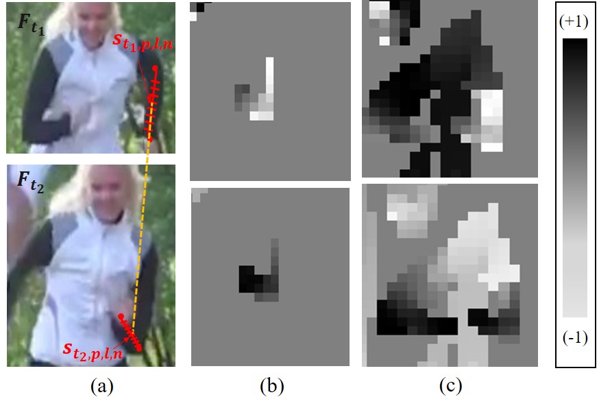
Figure 3: An example of TML (a) Illustration explaining how to obtain the TML using the frames $F_{t_{1}}$ and $F_{t_{2}}$. We subdivide each limb into several parts and calculate the unit vector of each pair (connected by the yellow lines, $S_{t_{1},p,l,n}$ and $S_{t_{2},p,l,n}$). (b) Visualization of the left arm TML on $x$(top) and $y$(bottom) coordinates. (c) Accumulated TML for all limbs on $x$(top) and $y$(bottom) coordinates. The values of TML are between the range of -1 and 1.

III-A Temporal flow Maps for Limb movement (TML)

The TML is a set of vector fields representing flows of person’s limbs. In this paper, a limb denotes a part linking two joints such as an upper arm and calf. An example of the vector fields of a single limb is shown in Figure 3(b). To obtain these new type of maps, first we divide each limb at regular intervals to multiple parts. Figure 3(a) shows an example of a divided limb at frame $F_{t_{1}}$ and $F_{t_{2}}$. In the figure, the red line means a limb and each yellow dot line shows the same parts on the same limb between frames. A separated part ($S_{t,p,l,n}$), which means an $n$-th separated part on $l$-th limb on the $p$-th person at the frame $t$, is used to calculate the movement direction between two frames. Based on the pair $(S_{t_{1},p,l,n},S_{t_{2},p,l,n})$, we calculate a unit vector $v$ as follows:

$$v=\frac{({S}_{t_{1},p,l,n}-{S}_{t_{2},p,l,n})}{\left\|{S}_{t_{1},p,l,n}-{S}_{t_{2},p,l,n}\right\|_{2}}.$$ (1)

Here, $n$, $l$ and $p$ represent the index of a separated part, a limb and a person respectively, and $t_{1}$ and $t_{2}$ are the frame indices. The part $S$ is represented by a two dimensional vector corresponding to the position of the part and thus $v$ is also a two-dimensional vector.

Then, the $L$ for the $l$-th limb is encoded through the unit vector $v$ for each pixel $s=(x,y)$ which is the limb passes through at the time interval $t_{1}$ and $t_{2}$. To draw the TML, we applied the similar process of part affinity field in [1].

$$L_{l,p}(s)=\left\{\begin{matrix}\begin{matrix}v&\textrm{if }~{}s\subseteq C\\ 0&\textrm{otherwise}.\end{matrix}\end{matrix}\right.$$ (2)

According to the condition ($C$), each pixel is determined to whether it is on the path of limb movement at the time interval $t_{1}$ and $t_{2}$. More concretely, in our case, the pixels belonging to the line segment ($S_{t_{1},p,l,n}$, $S_{t_{2},p,l,n}$) with a constant width is filled with the value of $v$ and the other pixels remain as zero.

When the TML of multi person are overlapped at the same position, it is averaged to preserve the scales of the output. Thus, the final TML for the $l$-th joint averages the TML of the joints of all people appeared in the image as follows:

$$L_{l}(s)=\begin{cases}\frac{1}{P(s)}\sum_{p=1}^{P(s)}L_{l,p}(s),&\quad\textrm{if }P(s)\geq 1\\ 0&\quad\textrm{if }P(s)=0,\end{cases}$$ (3)

where $P(s)$ means the number of non-zero vectors at pixel $s$. All of $n$ divided parts follow the above process to make the TML. Figure 3(b) shows a visualization of the TML of a single limb that is a part of left lower arm in $x$ and $y$ directions. The closer the value to $-1(+1)$, the brighter (darker) it becomes. In Figure 3(a), we can see that the left hand of the person moves to the left-down side. Then, the direction of $x$ channel is $-$ while the direction of $y$ channel becomes $+$ as shown in Figure 3(b). Thus, it is confirmed that the direction is different in each pixel of the TML.

Unlike optical flow [29] representing directions and magnitudes at each location, the TML only represents the directions using unit vectors. Because the TML does not contain magnitude information, it is more prone to change of time interval between frames. The multi-stride method for data augmentation, which will be describe in the next subsection, helps to alleviate this issue and successfully trains the network using video frames with different sampling rates.

Furthermore, the TML channel can be set as an individual channel for each limb (Figure 3(b)) or as an accumulated channel which accumulates the TML of all limbs (Figure 3(c)). The number of individual channels becomes the number of limbs $\times$ 2 ($x,y$ coordinate channel) while the accumulated channel has only 2 channels ($x,y$ coordinate channel). We will show the efficiency of different types of channel in the evaluation section.

III-B Multi-stride method

The TML has temporal information on the joint location. We need a huge dataset containing various situations and poses to learn the maps. If one trains the TML by using only a fixed time interval in videos sequentially, only limited types of maps can be obtained, which usually contains very small movements. Thus, we propose a multi-stride method which uses a pair of frames with various time interval as a data augmentation method. To generate the various time interval, we randomly select two frames within a given time range.

Figure 4 shows the examples of the TML on a small-motion video. If we only use the time interval of one shown in Figure 4(a), we cannot get a direction of large motions in this video. On the other hands, if we use various time intervals, additional maps can be obtained as shown in Figure 4(b) and (c), making it possible to express a case where the motion is varied even in a small movement.

Furthermore, our multi-stride method can be used to refine poses at inference time. The proposed refining method can be useful when a frame misses a person but the preceding and the next frames successfully target the person. In this case, because our multi-stride method randomly selected two frames at the training time and the network learned this situation, we can extract the TML and track the pose between frame $F_{t}$ and $F_{t+2}$. More details can be found in the Section III-C.

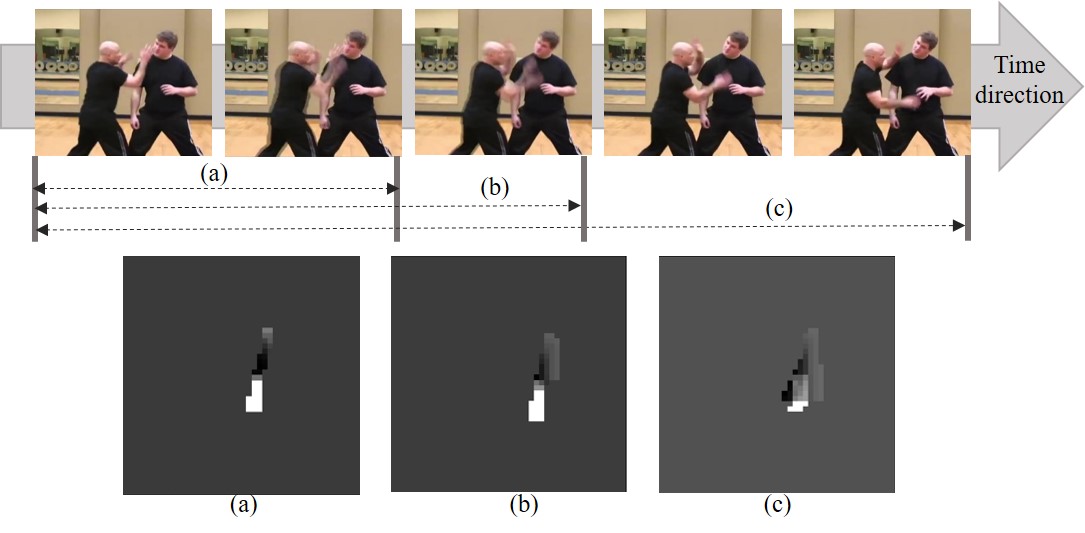
Figure 4: Examples of the TML of x coordinate with various time intervals. Consecutive image sequences are shown from left to right. (a), (b) and (c) are the right arm TML of the left person with the different time intervals, 1, 2 and 4 respectively. Using various strides, it is possible to get the TML of both small and large movements.

TABLE I: The estimation and tracking results of the proposed methods on the PoseTrack2017 and 2018 validation data. #stage means the number of stacked stages in the temporal part. Joint-Flow has a different type of temporal map that is created by joint movement. Basically, the proposed TML has two channels ($x$ and $y$) for each limb. ($*$) means the method in which the TML of all limbs are accumulated in a single map for x and y directions. $+$ adopted the non-maximum suppression (NMS) for joints. $++$ indicates that the proposed refining method for the middle frame pose is applied. Distance means that The TML is not used in the calculation of the association score in (4) by setting $\alpha$ to 0, which means that it only uses the torso distance of a person for the associated score.

data Method MOTA mAP #stage Head Shou Elb Wri Hip Knee Ankl Total Joint-Flow($*$) 1 70.6 70.1 50.6 37.5 53.9 41.8 30.3 52 73.1 Joint-Flow 1 48.5 48.3 30.3 19.3 33.9 23 13.5 32.1 73.2 TML($*$) 1 72 70.6 52.1 37.7 53.8 41.3 30.9 52.6 71.3 2017 TML 1 70.1 69.5 51.9 40.5 53.8 43.5 32.7 52.9 72.9 TML 3 74.7 74.1 61.7 49.4 59 52.6 43.7 60.3 70.9 TML+ 3 75.1 74.6 62.5 50.1 59.5 53 44.2 60.9 71.3 Distance+ 3 49.9 50.1 40.5 31.5 37.7 32.4 26.7 39.2 71.3 TML++ 3 75.5 75.1 62.9 50.7 60 53.4 44.5 61.3 71.5 2018 TML++ 3 76 76.9 66.1 56.4 65.1 61.6 52.4 65.7 74.6

III-C Inference

We define a set of frames consisting of three frames ($F_{t-1}$, $F_{t}$, $F_{t+1}$) as shown in Figure 1 for temporal inference which associates joint candidates in different frames. First, on each frame, we estimate the joint candidates using the joint heatmaps and spatially connect the candidates using part affinity fields as in [1]. The heatmaps and part affinity fields are created by the spatial part as shown in Figure 2.

Based on the connected joint candidates denoted as $I$, we track the poses. We calculate the associated score of each person in different frames. The associated score is calculated by a linear combination of a score of the TML ($S_{{\color[rgb]{0,0,0}T}}$) and a score of joint distance ($S_{d}$):

$$S=\alpha S_{{\color[rgb]{0,0,0}T}}+(1-\alpha)S_{d},$$ (4)

where $\alpha$ is a hyper-parameter which is set to 0.5 in our experiments.

We measure the score of a candidate movement on each TML by calculating the line integral. More specifically, we extract two joint candidates $I_{j}^{t_{1}}$ and $I_{j}^{t_{2}}$ in different frames at time $t_{1}$ and $t_{2}$ corresponding to the joint $j$ and make a normalized directional vector between the two joint candidates. Then the value of the TML corresponding to the line segment ($I_{j}^{t_{1}}$, $I_{j}^{t_{2}}$) is obtained to take inner product with the directional vector. This is done for all the points in the line segment and integrated as follows:

$$S_{{\color[rgb]{0,0,0}T}}=\frac{1}{n_{J}}\sum_{j=1}^{n_{J}}\int_{u=0}^{u=1}L_{l}(K(u))\cdot\frac{I_{j}^{t_{1}}-I_{j}^{t_{2}}}{\left\|I_{j}^{t_{1}}-I_{j}^{t_{2}}\right\|_{2}}du.$$ (5)

Here, $I$ is a joint candidate and $n_{J}$ is the number of joints for a person which is determined in the spatial part. $K(u)$ indicates interpolated points in the line segment ($I_{j}^{t_{1}}$, $I_{j}^{t_{2}}$) where $u\in\{0,1\}$, i.e., $K(u)=(1-u)\cdot I_{j}^{t_{1}}+u\cdot I_{j}^{t_{2}}$. This score measures the plausibility of joint association between frames using the TML.

We measured the joint distance ($S_{d}$) between the frames using the Euclidean distance.

$$S_{{\color[rgb]{0,0,0}d}}=\frac{1}{n_{J}}\sum_{j=1}^{n_{J}}\begin{Vmatrix}I_{j}^{t_{1}}-I_{j}^{t_{2}}\end{Vmatrix}$$ (6)

Both scores are given a different weight by using the variable $\alpha$ which is determined through experiments. Finally, we find the optimal connection by applying a bipartite graph [2].

After this, we refine the poses that have disappeared at the intermediate frame and come out again as shown in the second and the third images in Figure 1. More specifically, those situation means that the pose are not extracted on the frame $F_{t}$ but extracted and tracked between the frames $(F_{t-1},F_{t+1})$. To improve the situation, after pairs of frames with the time interval of one ($F_{t-1}$, $F_{t}$), ($F_{t}$, $F_{t+1}$) are processed, then to recover the missing person or joint in the frame $F_{t}$, a pair of frames with the time interval of two ($F_{t-1}$, $F_{t+1}$) is inputted to the proposed network followed by the above tracking method. After that, the poses or the joints missed in the middle of the frame $F_{t}$ are filled with average locations of those in $F_{t-1}$ and $F_{t+1}$.

IV Experiments

IV-A Datasets

In order to prove the efficiency of the proposed method, experiments on the PoseTrack 2017 and 2018 datasets [17] have been performed. PoseTrack datasets are large-scale benchmarks for human pose estimation and tracking. The PoseTrack datasets have various videos of human activities including fishing, running, tennis and so on. The datasets include a wide range of pose variations from a monotonous pose to a complex pose. PoseTrack datasets have the videos more than 500 sequences that are expected to be more than 20K frames. It is composed of 250 videos for training, 50 videos for validation and 214 videos for testing. PoseTrack 2018 dataset annotated more data than 2017.

The annotation types of PoseTrack 2017 and 2018 are different. The joints of PoseTrack 2018 added more parts such as ears and shoulder on top of the joints of PoseTrack 2017 and a new order of joints has been set. However, at the test time, mean average precision (mAP), multiple object tracker accuracy (MOTA) and multiple object tracking precision (MOTP) are evaluated in the annotation order of PoseTrack 2017.

IV-B Implementation details

We used the open-source library Caffe [30] to implement our model. Our model was trained with a weight decay of 0.0005, a momentum of 0.9 and a learning rate of 0.00005. We used the pre-trained model of [1] trained on COCO keypoints dataset [31] as a base network. At the training time, we needed to change the joint order and to add some parts such as ears to middle of head from Postrack to COCO to use the pre-trained model parameter, because COCO data and PoseTrack data have different order of joints.

At the training time, we applied data augmentation methods such as random crop, random rotate and so on. We set the scaling and rotation parameters based on the first frame among the two images. After a scaling and a rotation, we randomly select a person and crop a region such that the center of the selected person is located at the center of the region. The scaling, the rotation and selected person information of the first frame are applied equally in the second frame.

IV-C Evaluation

MOTA, MOTP and mAP are used to evaluate the performance [32]. Table I shows the results of the proposed methods by different settings - using different numbers (1 or 3) of iterative stages in the temporal part (#stage), using channel accumulation of TML instead of using individual channels for each joint ($*$), and a tracking method only using distance score by setting $\alpha$ in (4) as 0 (distance). Through the experiment, we empirically decide the number of subdivide each limb to 20 pieces to make the TML.

To make the temporal network part having as few parameters as possible while maintaining high performance, we experimented with different number of repetition stages, 1, 3 and 6. The spatial part used a fixed six stages. Table I only compares the performances with one and three iterative stages in the temporal part, because the experimental result of the iterative 6 stages is lower than that of 3 stages and has a huge number of parameters.

Similar to optical flow [29], we accumulate all limb movements in one map called accumulated channel map as shown in Figure 3(c). On the Table I, ($*$) means that the network used the accumulated TML. Basically, we use a map with a channel for each limb called individual channel map. The number of channel on individual channel map is (the number of $(x,y)$ channels = 2)$\times$(the number of limbs), but the accumulated channel map has only two $(x,y)$ channels. In all the tested networks, the accumulated channel map obtained lower accuracy than the individual channel map. Huge amount of the directional information of each limb is lost in the accumulated map, because the map includes some problems, e.g., different limbs overlap in the same location and have an averaging effect on that point.

TABLE II: Pose estimation and tracking performance on PoseTrack 2017 test dataset.

Method mAP MOTA MOTP Prec. Rec Top-down Poseflow[16] 63 51 16.9 71.2 78.9 MVIG 63.2 50.8 - - - Xiao et al.[15] 74.6 57.8 62.6 79.4 80.3 JointFlow[2] 63.6 53 23.2 82.1 70.6 Bottom-up Jin et al.[5] 59.16 50.59 - - - TML++ 68.78 54.46 85.2 80 76.1

TABLE III: Pose estimation and tracking performance on PoseTrack 2018 test dataset.

Method Additional training data MOTA mAP Wrists AP Ankles AP Xiao et al. [15] +COCO+Other 61.37 74.03 73 69.05 ALG +COCO+Other 60.79 74.85 72.62 71.11 Miracle +COCO+Other 57.36 70.9 68.19 66.06 CMP +COCO 54.47 64.67 61.78 60.86 PR +COCO 44.54 59.05 50.16 49.4 TML++ +COCO 54.86 67.81 60.2 56.85

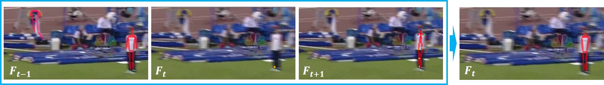
Figure 5: An example of pose refinement using multi-stride inputs during the inference. The person at the right side of input images (red line) is tracked from $F_{t-1}$ to $F_{t+1}$, but the pose of the person is not detected at $F_{t}$. By associating the poses at $F_{t-1}$ and $F_{t+1}$, we can retrieve the missed pose at $F_{t}$. On the other hand, we cannot refine the person on the left side (pink line), because it is only estimated at the $F_{t-1}$.

Figure 6: The qualitative results of the proposed multi-stride pose estimator and tracker. The images are in chronological order from left to right. Tracked poses are displayed in the same color.

We implemented and compared the performance of the Joint-Flow map to show that the map created using limbs is more efficient than the map created using joints. The Joint-Flow map is constructed as a direction in which the joint moves between two frames. The Joint-Flow map follows the equation of (2) but uses the joint location instead of separated part $s$. The mAPs of Joint-Flow are higher than the TML , but MOTAs are lower. This results shows the difficulty of tracking using the Joint-Flow, because the Joint-Flow map has less information than the TML. Moreover, we compared with JointFlow [2] that proposed a temporal map about joint movement as shown in Table II. On the PoseTrack 2017 test set, our results are better than those of the JointFlow [2].

Because the proposed method is the bottom-up approach, it is possible to detect many joint candidates on the same part. Thus, a non-maximum suppression (NMS) is applied for joints to reduce confusion after estimating joint location. (+) in Table I means that first we detect joints using the joint heatmaps and refine the joint using NMS. Reducing the confusing candidates increases tracking performance by around 0.4% in mAP and 0.6% in MOTA.

The sum of the TML score and the joint distance score is used for the association score to track poses. We experimented to see how the joint distance affects to association score. On Table I, (Distance) means that only joint distances of a person is used in the calculation of association score. To enable this, at inference time, we use the same structure as TML+ and set $\alpha$ to $0$. Only using the distance score incurs more confusion with nearby people and the resultant MOTA is by far lower than others on average. However, we need to use the distance score to handle the case of no motion. Thus, we apply $\alpha$ to $0.5$ in all the other cases.

One of our contributions is the refining method for the middle frame pose. We refine the pose on the middle of frame by analyzing between three frames. (++) in Table I, Table II, and Table III means that the refining method is applied. Figure 5 shows an example result of the refined pose. The pose on $F_{t}$ is refined through the association between frames $F_{t-1}$ and $F_{t+1}$. In case of the person on the right side (red line), the person is tracked at the $F_{t-1}$ and the $F_{t+1}$, but not tracked at the $F_{t}$. Through the refining method, an average pose between $F_{t-1}$ and $F_{t+1}$ is added on the frame $F_{t}$. Unfortunately, the person on the left side (pink line) can not be tracked through the refining method, because the pose is not estimated at the $F_{t+1}$.

Figure 6 shows qualitative results of pose estimation and tracking. Poses are estimated and tracked well in a variety of environments even when several people move close together or quickly. Because our association score considers the distance score, poses that have a little movement can also be tracked as shown in the fourth row on Figure 6. Unfortunately, if the poses nearly occludes each other as in the last row of Figure 6, the pose is likely to be missed. For future work, we may propagate the pose through the TML and refine the estimated pose by comparing it with the propagated pose to address this.

We compare our method with the state-of-the-art methods on the PoseTrack 2017 and 2018 test datasets as shown in Table II. Though the proposed method shows a lower performance than the highest record [15], the result of the proposed network is the best among the bottom-up approaches.

Because the PoseTrack challenge was held on the September 2018, papers using the PoseTrack 2018 data have not been published yet. We could not compare the proposed method with other methods on the PoseTrack 2018 validate data. However, we can compare results of state-of-the-art on the PoseTrack 2018 test data through the results on the PoseTrack leader-board site as shown in the Table III. We cannot compare the structures of the networks, but ours shows the best performance among the ones trained only using COCO data.

V Conclusions

We propose a multi-stride pose estimator and tracker. It tracks the joints based on the TML which is a unit vector map representing the human flow. The multi-stride method has been used to train various temporal flow maps. Our method utilizes both the spatial and temporal information. Spatial information such as joint heatmaps and part affinity fields is regressed by the spatial part and TML is regressed by the temporal part. The combined network can be trained in an end-to-end manner influencing each other. We demonstrate the efficiency of the proposed method on the PoseTrack 2017 and 2018 datasets.

References

- [1] Z. Cao, T. Simon, S.-E. Wei, and Y. Sheikh, “Realtime multi-person 2d pose estimation using part affinity fields,” CVPR, 2017.
- [2] A. Doering, U. Iqbal, and J. Gall, “Joint flow: Temporal flow fields for multi person tracking,” BMVC, 2018.
- [3] E. Insafutdinov, L. Pishchulin, B. Andres, M. Andriluka, and B. Schiele, “Deepercut: A deeper, stronger, and faster multi-person pose estimation model,” in ECCV, 2016, pp. 34–50.
- [4] U. Iqbal, A. Milan, and J. Gall, “Posetrack: Joint multi-person pose estimation and tracking,” in CVPR, 2017.
- [5] S. Jin, X. Ma, Z. Han, Y. Wu, W. Yang, W. Liu, C. Qian, and W. Ouyang, “Towards multi-person pose tracking: Bottom-up and top-down methods,” in ICCV PoseTrack Workshop, 2017.
- [6] G. Ning and Z. He, “Dual path networks for multi-person human pose estimation,” in ICCV PoseTrack Workshop, 2017.
- [7] L. Pishchulin, E. Insafutdinov, S. Tang, B. Andres, M. Andriluka, P. Gehler, and B. Schiele, “Deepcut: Joint subset partition and labeling for multi person pose estimation,” in CVPR, 2016.
- [8] I. Radwan, A. Asthana, and R. Geocke, “Global pose refinement using bidirectional long-short term memory,” https://posetrack.net/workshops/iccv2017/pdfs/MPR.pdf.
- [9] F. Xia, P. Wang, X. Chen, and A. L. Yuille, “Joint multi-person pose estimation and semantic part segmentation,” in CVPR, 2017, pp. 6080–6089.
- [10] X. Zhu, Y. Jiang, and Z. Luo, “Multi-person pose estimation for posetrack with enhanced part affinity fields,” in ICCV PoseTrack Workshop, 2017.
- [11] H.-S. Fang, S. Xie, Y.-W. Tai, and C. Lu, “RMPE: Regional multi-person pose estimation,” in ICCV, 2017.
- [12] R. Girdhar, G. Gkioxari, L. Torresani, M. Paluri, and D. Tran, “Detect-and-Track: Efficient Pose Estimation in Videos,” in CVPR, 2018.
- [13] A. Newell, Z. Huang, and J. Deng, “Associative embedding: End-to-end learning for joint detection and grouping,” in NIPS, 2017, pp. 2274–2284.
- [14] G. Papandreou, T. Zhu, N. Kanazawa, A. Toshev, J. Tompson, C. Bregler, and K. Murphy, “Towards accurate multi-person pose estimation in the wild,” in CVPR, 2017, pp. 3711–3719.
- [15] B. Xiao, H. Wu, and Y. Wei, “Simple baselines for human pose estimation and tracking,” ECCV, 2018.
- [16] Y. Xiu, J. Li, H. Wang, Y. Fang, and C. Lu, “Pose flow: Efficient online pose tracking,” BMVC, 2018.
- [17] M. Andriluka, U. Iqbal, E. Ensafutdinov, L. Pishchulin, A. Milan, J. Gall, and S. B., “PoseTrack: A benchmark for human pose estimation and tracking,” in CVPR, 2018.
- [18] A. Bulat and G. Tzimiropoulos, “Human pose estimation via convolutional part heatmap regression,” in ECCV, 2016.
- [19] Y. Chen, C. Shen, X.-S. Wei, L. Liu, and J. Yang, “Adversarial PoseNet: A structure-aware convolutional network for human pose estimation,” in ICCV, 2017.
- [20] X. Chu, W. Yang, W. Ouyang, C. Ma, A. L. Yuille, and X. Wang, “Multi-context attention for human pose estimation,” CVPR, pp. 5669–5678, 2017.
- [21] A. Newell, K. Yang, and J. Deng, “Stacked hourglass networks for human pose estimation.”
- [22] V. Ramakrishna, D. Munoz, M. Hebert, J. Andrew Bagnell, and Y. Sheikh, “Pose machines: Articulated pose estimation via inference machines,” in ECCV 2014, 2014, pp. 33–47.
- [23] J. Tompson, R. Goroshin, A. Jain, Y. LeCun, and C. Bregler, “Efficient object localization using convolutional networks,” in CVPR, 2015, pp. 648–656.
- [24] J. Tompson, A. Jain, Y. LeCun, and C. Bregler, “Joint training of a convolutional network and a graphical model for human pose estimation,” in NIPS, 2014, pp. 1799–1807.
- [25] S.-E. Wei, V. Ramakrishna, T. Kanade, and Y. Sheikh, “Convolutional pose machines,” in CVPR, 2016, pp. 4724–4732.
- [26] W. Yang, S. Li, W. Ouyang, H. Li, and X. Wang, “Learning feature pyramids for human pose estimation,” in ICCV, 2017, pp. 1290–1299.
- [27] E. Insafutdinov, M. Andriluka, L. Pishchulin, S. Tang, E. Levinkov, B. Andres, and B. Schiele, “ArtTrack: Articulated Multi-person Tracking in the Wild,” in CVPR, 2017.
- [28] K. Simonyan and A. Zisserman, “Very deep convolutional networks for large-scale image recognition,” arXiv preprint arXiv:1409.1556, 2014.
- [29] B. K. Horn and B. G. Schunck, “Determining optical flow,” Artificial intelligence, vol. 17, no. 1-3, pp. 185–203, 1981.
- [30] Y. Jia, E. Shelhamer, J. Donahue, S. Karayev, J. Long, R. Girshick, S. Guadarrama, and T. Darrell, “Caffe: Convolutional architecture for fast feature embedding,” arXiv preprint arXiv:1408.5093, 2014.
- [31] T.-Y. Lin, M. Maire, S. Belongie, J. Hays, P. Perona, D. Ramanan, P. Dollár, and C. L. Zitnick, “Microsoft coco: Common objects in context,” in ECCV, 2014.
- [32] A. Milan, L. Leal-Taixé, I. Reid, S. Roth, and K. Schindler, “Mot16: A benchmark for multi-object tracking,” arXiv preprint arXiv:1603.00831, 2016.