Teleoperator Imitation with Continuous-time Safety

Abstract

Learning to effectively imitate human teleoperators, with generalization to unseen and dynamic environments, is a promising path to greater autonomy enabling robots to steadily acquire complex skills from supervision. We propose a new motion learning technique rooted in contraction theory and sum-of-squares programming for estimating a control law in the form of a polynomial vector field from a given set of demonstrations. Notably, this vector field is provably optimal for the problem of minimizing imitation loss while providing continuous-time guarantees on the induced imitation behavior. Our method generalizes to new initial and goal poses of the robot and can adapt in real-time to dynamic obstacles during execution, with convergence to teleoperator behavior within a well-defined safety tube. We present an application of our framework for pick-and-place tasks in the presence of moving obstacles on a 7-DOF KUKA IIWA arm. The method compares favorably to other learning-from-demonstration approaches on benchmark handwriting imitation tasks.

I Introduction

Teleoperation is enabling robotic systems to become pervasive in settings where full autonomy is currently out of reach [18, 47, 15]. Compelling applications include minimally invasive surgery [44, 45], space exploration [46], remote vehicle operations [16] and disaster relief scenarios [34]. A human teleoperator can control a robot through tasks that have complex semantics and are currently difficult to explicitly program or to learn to solve efficiently without supervision.

A downside of teleoperation is that it requires continuous error-free [7] operator attention even for highly repetitive tasks. This problem can be addressed through Learning-from-Demonstrations (LfD) or Imitation Learning techniques [41, 9] where a control law needs to be inferred from a small number of demonstrations. Such a law can then bootstrap data-efficient reinforcement learning for challenging tasks [47]. The demonstrator attempts to ensure that the robot’s motions capture the relevant semantics of the task rather than requiring the robot to understand the semantics. The learnt control law should take over from the teleoperator and enable the robot to repeatedly execute the desired task even in dynamically changing conditions. For example, the origin of a picking task and the goal of a placing task may dynamically shift to configurations unseen during training, and moving obstacles may be encountered during execution. The latter is particularly relevant in collaborative human-robot workspaces where safety guarantees are paramount. In such situations, when faced with an obstacle, the robot cannot follow the demonstration path anymore and needs to recompute a new motion trajectory in real-time to avoid collision and still attempt to accomplish the desired task.

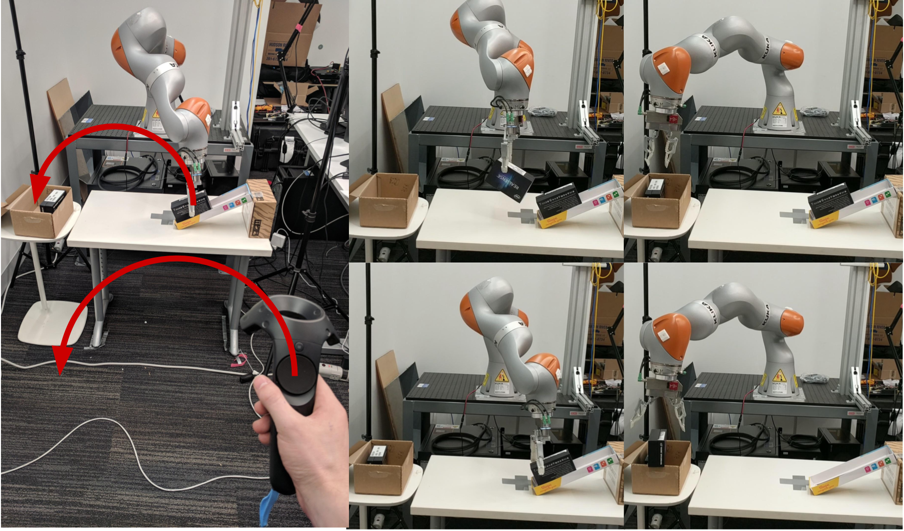
(a) Pick and place teleoperation demonstration

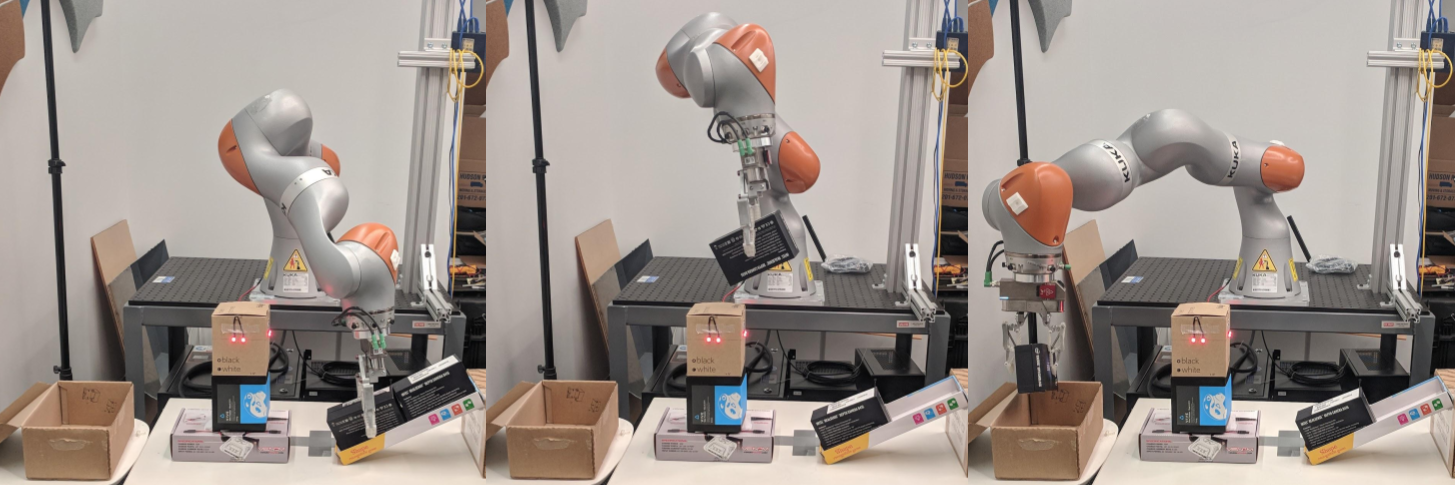
(b) Pick and place via contracting vector fields with obstacle avoidance.

Figure 1: (a) A non-technical user provides a demonstrates via teleoperation to accomplish a pick and place task. (b) The robot now autonomously executes the pick and place task with a contracting vector field (CVF) allowing for continuous time guarantees while also avoiding obstacles.

Such real-time adaptivity can be elegantly achieved by associating demonstrations with a dynamical system [40, 43, 25, 24, 27]: a vector field defines a closed-loop velocity control law. From any state that the robot finds itself in, the vector field can then steer the robot back towards the desired imitation behavior, without the need for path replanning with classical approaches. Furthermore, the learnt vector field can be modulated in real-time [26, 19, 28] in order to avoid collisions with obstacles.

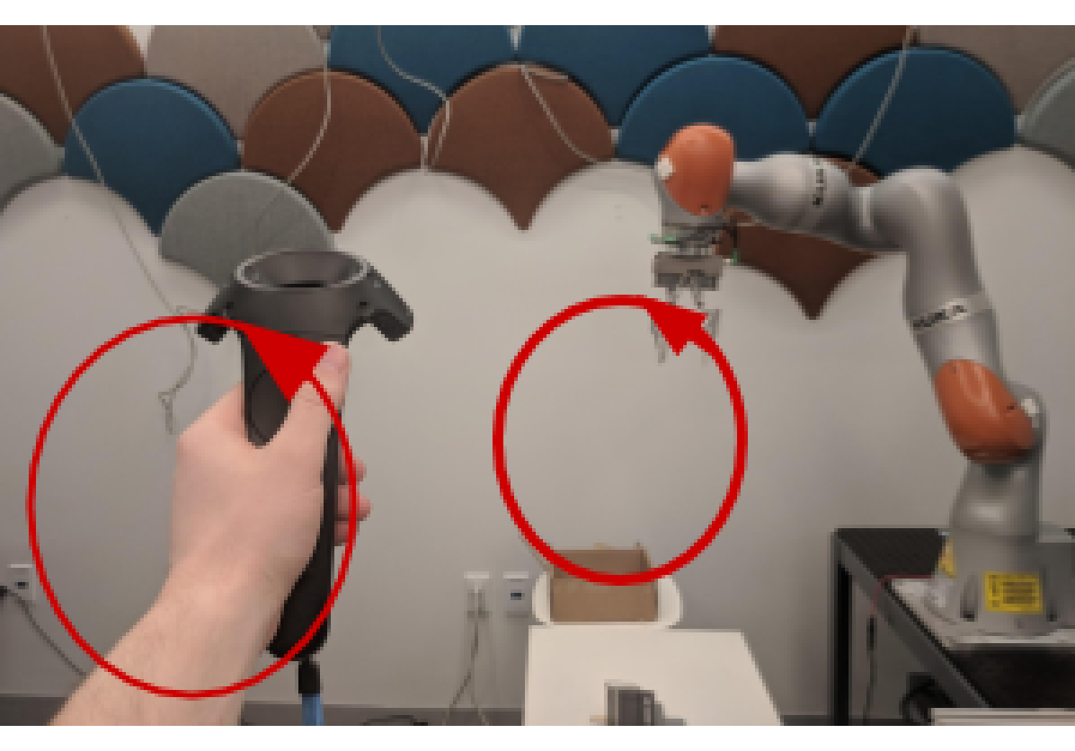
(a) Demo trajectory ${{\bf x}^{\text{sample}}}(t)$ started at (1,1)

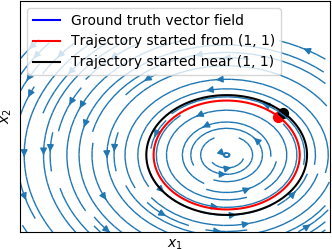
(b) True Vector Field $f^{\text{real}}$

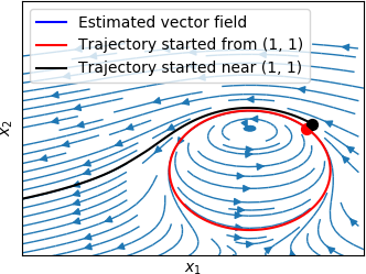
(c) Estimated vector field $f^{*}$

Figure 2: (a) a non-technical user demonstrates a circular trajectory. (b) the “ground truth” vector field. (c) the estimated vector field. Both vector fields produce the same trajectory when started from $(1,1)^{T}$ while they exhibit radically different behavior when started from a point arbitrarily close to $(1,1)^{T}$.

At first glance, the problem of imitation learning of a smooth dynamical system, $\dot{{\bf x}}=f({\bf x})$ from samples $({\bf x},\dot{{\bf x}})$ appears to be a straightforward regression problem: simply minimize imitation loss $\sum_{i,t}\|f({\bf x}^{(i)}(t))-\dot{\bf x}^{(i)}(t)\|_{2}^{2}$ over a suitable family of vector valued maps, $f\in{\cal F}$. However, a naive supervised regression approach may be woefully inadequate, as illustrated in the middle panel of Figure 2 where the goal is to have a KUKA arm imitate a circular trajectory. As can be seen, estimating vector fields from a small number of trajectories potentially leads to instability – the estimated field easily diverges when the initial conditions are even slightly different from those encountered during training. Therefore, unsurprisingly, learning with stability constraints has been the technical core of existing dynamical systems based LfD approaches, e.g. see [24, 27, 40, 43]. However, these methods have one or more of the following limitations: (1) they involve non-convex optimization for dynamics fitting and constructing Lyapunov stability certificates respectively and, hence, have no end-to-end optimality guarantees, (2) the notion of stability is not trajectory-centric, but rather focused on reaching a single desired equilibrium point, and (3) they are computationally infeasible when formulated in continuous-time. With this context, our contributions in this paper include the following:

• We formulate a novel continuous time optimization problem over vector fields involving an imitation loss subject to a generalization-enforcing constraint that turns the neighborhood of demonstrations into contracting regions [32]. Within this region, all trajectories are guaranteed to coalesce towards the demonstration exponentially fast.

• We show that our formulation leads to an instance of time-varying semidefinite programming [3] for which a sum-of-squares relaxation [30, 37, 6] turns out to be exact! Hence, we can find the globally optimal polynomial vector field that has the lowest imitation loss among all polynomial vector fields of a given degree that are contracting on a region around the demonstrations in continuous time.

• On benchmark handwriting imitation tasks [1], our method outperforms competing approaches in terms of a variety of imitation quality metrics.

• We demonstrate our methods on a 7DOF KUKA pick-and-place LfD task where task completeness is accomplished despite dynamic obstacles in the environment, changing initial poses and moving destinations. By contrast, without contraction constraints, the vector field tends to move far from the demonstrated trajectory activating emergency breaks on the arm and failing to complete the task.

Our “dirty laundry” includes: (1) we cannot handle high degree polynomials due to the scalability limitations of current SDP solvers, and (2) our notion of incremental stability is local, even though our method generalizes well in the sense that a wide contraction tube is setup around the demonstrations.

II Problem Statement

We are interested in estimating an unknown continuous time autonomous dynamical system

$$\dot{{\bf x}}=f^{\text{real}}({\bf x}),$$ (1)

where $f^{\text{real}}:\mathbb{R}^{n}\rightarrow\mathbb{R}^{n}$ is an unknown continuously differentiable function.

We assume that we have access to one or several sample trajectories ${\bf x}^{(i)}:~{}[0,T]~{}\mapsto~{}\mathbb{R}^{n}$ that satisfy $\dot{\bf x}^{(i)}=f^{\text{real}}({\bf x}^{(i)})\;\forall t\in[0,T]$, where $T>0$ and $i=1,\ldots,M$. These trajectories (${\bf x}^{(i)}$, for $i=1\ldots,M$) constitute our training data, and our goal is to search for an approximation of the vector field $f^{\text{real}}$ in a class of functions of interest $\mathcal{F}$ that reproduces trajectories as close as possible to the ones observed during training. In other words, we seek to solve the following continuous time least squares optimization problem (LSP):

$$f^{*}\in\arg\min_{f\in\mathcal{F}}\sum_{i=1}^{M}\int_{t=0}^{T}\|f({\bf x}^{(i)}(t))-\dot{\bf x}^{(i)}(t)\|_{2}^{2}\;\;{\rm d}t.$$ (LSP)

In addition to consistency with $f^{\text{real}}$, we want our learned vector field $f$ to generalize in conditions that were not seen in the training data. Indeed, the LSP problem generally admits multiple solutions, as it only dictates how the vector field should behave on the sample trajectories. This under-specification can easily lead to overfitting, especially if the class of function $\mathcal{F}$ is expressive enough. The example of Figure 2 reinforces this phenomenon even for a simple circular motion. Note that standard data-independent regularization (e.g., $L_{2}$ regularizer) is insufficient to resolve the divergence illustrated here: a stronger stabilizer ensuring convergence, not just smoothness, of trajectories is needed. The notion of stability of interest to us in this paper is contraction which we now briefly review.

II-A Incremental Stability and Contraction Analysis

Notions of stability called incremental stability and associated contraction analysis tools [21, 32] are concerned with the convergence of system trajectories with respect to each other, as opposed to classical Lyapunov stability which is with respect to a single equilibrium. Contraction analysis derives sufficient and necessary conditions under which the displacement between any two trajectories will go to zero. We give in this section a brief presentation of this notion based on [8].

Contraction analysis of a system $\dot{\bf x}=f({\bf x})$ is best explained by considering the dynamics of $\delta{\bf x}(t)$, the infinitesimal displacement between two trajectories:

$$\delta\dot{\bf x}=\mathbf{J}_{f}({\bf x})\delta{\bf x}\text{ where }\mathbf{J}_{f}({\bf x})=\frac{\partial}{\partial{\bf x}}f.$$

From this equation we can easily derive the rate of change of the infinitesimal squared distance between two trajectories $\|\delta{\bf x}\|_{2}^{2}=\delta{\bf x}^{T}\delta{\bf x}$ as follows:

$$\frac{{\rm d}}{{\rm d}t}\|\delta{\bf x}\|_{2}^{2}=2\delta{\bf x}^{T}\delta\dot{\bf x}=2\delta{\bf x}^{T}\mathbf{J}_{f}({\bf x})\delta{\bf x}.$$ (2)

More generally, we can consider the infinitesimal squared distance with respect to a metric that is different from the Euclidian metric. A metric is given by smooth, matrix-valued function ${\bf M}:{\mathbb{R}}^{+}\times{\mathbb{R}}^{n}\mapsto{\mathbb{R}}^{n\times n}$ that is uniformly positive definite, i.e. there exists $\varepsilon>0$ such that

$${\bf M}(t,{\bf x})\succeq\varepsilon\mathbf{I}\quad\forall t\in{\mathbb{R}}^{+},\;\forall{\bf x}\in{\mathbb{R}}^{n},$$ (3)

where $\mathbf{I}$ is the identity matrix and the relation $A\succeq B$ between two symmetric matrices $A$ and $B$ is used to denote that the smallest eigenvalue of their difference $A-B$ is nonnegative. For the clarity of presentation, we only consider metric functions ${\bf M}({\bf x})$ that do not depend on time $t$.

The squared norm of an infinitesimal displacement between two trajectories with respect to this metric is given by ${\|\delta{\bf x}\|_{{\bf M}({\bf x})}}^{2}\coloneqq\delta{\bf x}^{T}{\bf M}({\bf x})\delta{\bf x}$. The Euclidean metric corresponds to the case where ${\bf M}({\bf x})$ is constant and equal to the identity matrix.

Similarly to (2), the rate of change of the squared norm of an infinitesimal displacement with respect to a metric ${\bf M}({\bf x})$ follows the following dynamics:

$$\frac{{\rm d}}{{\rm d}t}{\|\delta{\bf x}\|_{{\bf M}({\bf x})}}^{2}=\delta{\bf x}^{T}(\operatorname{{\bf sym}}[{\bf M}({\bf x})\mathbf{J}_{f}({\bf x})]+\dot{\bf M}({\bf x}))\delta{\bf x},$$ (4)

where $\operatorname{{\bf sym}}[M]$ denotes $(M+M^{T})/2$ for any square matrix $M$ and $\dot{\bf M}({\bf x})$ is the $n\times n$ matrix whose $(i,j)\text{-entry}$ is $\nabla{\bf M}_{ij}({\bf x})^{T}f({\bf x})$. This motivates the following definition of contraction.

Definition 1 (Contraction)

For a positive constant $\tau$ and a subset $U$ of ${\mathbb{R}}^{n}$ the system $\dot{\bf x}=f({\bf x})$ is said to be $\tau\text{-\it{contracting}}$ on the region $U$ with respect to a metric ${\bf M}({\bf x})$ if

$$\operatorname{{\bf sym}}[{\bf M}({\bf x})\mathbf{J}_{f}({\bf x})]+\dot{\bf M}({\bf x})\preceq-\tau{\bf M}({\bf x})\quad\forall{\bf x}\in U.$$ (5)

Remark 1

When the vector field $f$ is a linear function $\dot{{\bf x}}=A{\bf x}$, and the metric ${\bf M}({\bf x})$ is constant ${\bf M}({\bf x})=P$, it is easy to see that contraction condition (5) is in fact equivalent to global stability condition,

$$P\succ 0\text{ and }{\operatorname{{\bf sym}}(PA^{T})\preceq-\tau P.}$$ (6)

Given a $\tau\text{-\it{contracting}}$ vector field with respect to a metric ${\bf M}({\bf x})$, we can conclude from the dynamics in (4) that

$$\frac{{\rm d}}{\;{\rm d}t}{\|\delta{\bf x}\|_{{\bf M}({\bf x})}}^{2}\leq-\tau{\|\delta{\bf x}\|_{{\bf M}({\bf x})}}$$

Integrating both sides yields,

$${\|\delta{\bf x}\|_{{\bf M}({\bf x})}}\leq e^{-\frac{\tau}{2}t}{\|\delta{\bf x}(0)\|_{{\bf M}({\bf x})}}$$

Hence, any infinitesimal length ${\|\delta{\bf x}\|_{{\bf M}({\bf x})}}$ (and by assumption (3), $\|\delta{\bf x}\|_{2}$) converges exponentially to zero as time goes to infinity. This implies that in a contraction region, trajectories will tend to converge together towards a nominal path. If the entire state-space is contracting and a finite equilibrium exists, then this equilibrium is unique and all trajectories converge to this equilibrium.

In the next section, we explain how to globally solve the following continuous-time vector field optimization problem to fit a contracting vector field to the training data given some fixed metric ${\bf M}({\bf x})$. We refer to this as the least squares problem with contraction (LSPC):

$$\min_{f\in\mathcal{F}} \sum_{i=1}^{M}\int_{t=0}^{T}\|f({\bf x}^{(i)}(t))-\dot{{\bf x}^{(i)}}(t)\|^{2}_{2}\;\;{\rm d}t$$ (LSPC)

s.t. $$f U\subseteq{\mathbb{R}}^{n}$$ is contracting on a region

containing the demonstrations $${\bf x}^{(i)}(t)$$

with respect to the metric $${\bf M}({\bf x})$$.

The search for a contraction metric itself may be interpreted as the search for a Lyapunov function of the specific form $V({\bf x})=f({\bf x})^{T}\mathbf{M}({\bf x})f({\bf x})$. As is the case with Lyapunov analysis in general, finding such an incremental stability certificate for a given dynamical system is a nontrivial problem; see [8] and references therein. If one wishes to find the vector field and a corresponding contraction metric at the same time, then the problem becomes non-convex. A common approach to handle this kind of problems is to optimize over one parameter at a time and fix the other one to its latest value and then alternate (i.e. fix a contraction metric and fit the vector field, then fix the vector field and improve on the contraction metric.)

III Learning Contracting Vector Fields as a Time-Varying Convex Problem

In this section we explain how to formulate and solve the problem of learning a contracting vector field from demonstrations described in (LSPC). We will first see that we can formulate it as a time-varying semidefinite problem. We will then describe how to use tools from sum of squares programming to solve it.

III-A Time-Varying Semidefinite Problems

We call time-varying semidefinite problems (TV-SDP) optimization programs of the form

$$\min_{f\in\mathcal{F}} \quad L(f)$$ (TV-SDP)

s.t. $$\quad\mathcal{L}_{i}f(t)\succeq 0\quad\forall i=1,\ldots,m\;\forall t\in[0,T],$$

where the variable $t\in[0,T]$ stands for time, the loss function $L:\mathcal{F}\mapsto{\mathbb{R}}$ in the objective is assumed to be convex and the $\mathcal{L}_{i}$ ($i=1,\ldots,m$) are linear functionals that map an element $f\in\mathcal{F}$ to a matrix-valued function $\mathcal{L}_{i}f:[0,T]\mapsto{\mathbb{R}}^{n\times n}$. We will restrict the space of functions $\mathcal{F}$ to be the space of functions whose components are polynomials of degree $d\in\mathbb{N}$:

$$\mathcal{F}\coloneqq\{f:{\mathbb{R}}^{n}\mapsto{\mathbb{R}}^{n}\;|\;f_{i}\in{\mathbb{R}}_{d}[{\bf x}]\},$$ (7)

and we make the assumption that $\mathcal{L}_{i}f$ is a matrix with polynomial entries. Our interest in this setting stems from the fact that polynomial functions can approximate most functions reasonably well. Moreover, polynomials are suitable for algorithmic operations as we will see in the next section. See [3] for a more in-depth treatment of time-varying semidefinite programs with polynomial data.

Let us now show how to reformulate the problem in (LSPC) of fitting a vector field $f:{\mathbb{R}}^{n}\mapsto{\mathbb{R}}^{n}$ to $m$ sample trajectories $\{({\bf x}^{(i)}(t),\dot{\bf x}^{(i)}(t))\;|\;t\in[0,T],\;i=1,\ldots,m\}$ as a (TV-SDP). For this problem to fit within our framework, we start by approximating each trajectory ${\bf x}^{(i)}(t)$ with a polynomial function of time ${\bf x}^{(i)}_{\text{poly}}(t)$. Our decision variable is the polynomial vector field $f$ and we seek to optimize the following objective function

$$L(f)\coloneqq\sum_{i=1}^{M}\int_{t=0}^{T}\|f({\bf x}^{(i)}_{\text{poly}}(t))-\dot{\bf x}^{(i)}_{\text{poly}}(t)\|^{2}_{2}\;{\rm d}t$$ (8)

which is already convex (in fact convex quadratic). In order to impose the contraction of the vector field $f$ over some region around the trajectories in demonstration, we use a smoothness argument to claim that it is sufficient to impose contraction only on the trajectories themselves. See Proposition 1 later for a more quantitative statement of this claim. To be concrete, we take

$$\mathcal{L}_{i}f(\cdot)\coloneqq -\operatorname{{\bf sym}}[{\bf M}({\bf x}^{(i)}_{\text{poly}}(\cdot))\mathbf{J}_{f}({\bf x}^{(i)}_{\text{poly}}(\cdot))]$$

$$-\dot{\bf M}({\bf x}^{(i)}_{\text{poly}}(\cdot))-\tau{\bf M}({\bf x}^{(i)}_{\text{poly}}(\cdot)),$$ (9)

where ${\bf M}({\bf x})$ is some known contraction metric.

III-B Sum-Of-Squares Programming

In this section we review the notions of sum-of-squares (SOS) programming and its applications to polynomial optimization, and how we apply it for learning a contracting polynomial vector field. SOS techniques have found several applications in Robotics: constructing Lyapunov functions [2], locomotion planning [39], design and verification of provably safe controllers [33], grasping and manipulation [13], inverse optimal control [38] and modeling 3D geometry [4].

Let ${\mathbb{R}}_{d}[{\bf x}]$ be the ring of polynomials $p({\bf x})$ in real variables ${\bf x}=(x_{1},\ldots,x_{n})$ with real coefficients of degree at most $d$. A polynomial $p\in{\mathbb{R}}[{\bf x}]$ is nonnegative if $p({\bf x})\geq 0$ for every ${\bf x}\in{\mathbb{R}}^{n}$. In many applications, including the one we cover in this paper, we seek to find the coefficients of one (or several) polynomials without violating some nonnegativity constraints. While the notion of nonnegativity is conceptually easy to understand, even testing whether a given polynomial is nonnegative is known to be NP-hard as soon as the degree $d\geq 4$ and the number of variables $n\geq 3$.

A polynomial $p\in{\mathbb{R}}_{d}[{\bf x}]$, with $d$ even, is a sum-of-squares (SOS) if there exists polynomials $q_{1},\ldots,q_{m}\in{\mathbb{R}}_{\frac{d}{2}}[{\bf x}]$ such that

$$p({\bf x})=\sum_{i=1}^{m}q_{i}({\bf x})^{2}.$$ (10)

An attractive feature of the set of SOS polynomials is that optimizing over it can be cast as a semidefinite program of tractable size, for which many solvers already exist. Indeed, it is known [30][37] that a polynomial $p({\bf x})$ of degree $d$ can be decomposed as in (10) if and only if there exists a positive semidefinite matrix $Q$ such that

$$p({\bf x})=z({\bf x})^{T}Qz({\bf x})\;\forall{\bf x}\in{\mathbb{R}}^{n},$$

where $z({\bf x})$ is the vector of monomials of ${\bf x}$ up to degree $\frac{d}{2}$, and the equality between the two sides of the equation is equivalent to a set of linear equalities in the coefficients of the polynomial $p({\bf x})$ and the entries of the matrix $Q$.

Sum-of Squares Matrices: If a polynomial $p({\bf x})$ is SOS, then it is obviously nonnegative, and the matrix $Q$ acts as a certificate of this fact, making it easy to check that the polynomial at hand is nonnegative for every value of the vector ${\bf x}$. In order to use similar techniques to impose contraction of a vector field, we need a slight generalization of this concept to ensure that a matrix-valued polynomial $P({\bf x})$ (i.e. a matrix whose entries are polynomial functions) is positive semidefinite (PSD) for all values of ${\bf x}$. We can equivalently consider the scalar-valued polynomial $p({\bf x},{\bf u})\coloneqq{\bf u}^{T}P({\bf x}){\bf u}$, where ${\bf u}$ is a $n\times 1$ vector of new indeterminates, as positive semidefiniteness of $P({\bf x})$ is equivalent to the nonnegativity of $p({\bf x},{\bf u})$. If $p({\bf x},{\bf u})$ is SOS, then we say that $P$ is a sum-of-squares matrix (SOSM) [29, 17, 42]. Consequently, optimizing over SOSM matrices is a tractable problem.

Exact Relaxation: A natural question here is how much we lose by restricting ourselves to the set of SOSM matrices as opposed the set of PSD matrices. In general, these two sets are quite different [10]. In our case however, all the matrices considered are univariate as they depend only on the variable of time $t$. It turns out that, in this special case, these two notions are equivalent!

Theorem 1 (See e.g. [11])

A matrix-valued polynomial $P(t)$ is PSD everywhere (i.e. $P(t)\succeq 0\;\forall t\in{\mathbb{R}}$) if and only if the associated polynomial $p(t,{\bf u})\coloneqq{\bf u}^{T}P(t){\bf u}$ is SOS.

The next theorem generalizes this result to the case where we need to impose PSD-ness only on the interval $[0,T]$ (as opposed to $t\in{\mathbb{R}}$.)

Theorem 2 (See Theorem 2.5 of [14])

A matrix-valued polynomial $P(t)$ of degree $d$ is PSD on the interval $[0,T]$ (i.e. $P(t)\succeq 0\;\forall t\in[0,T]$) if and only if can be written as

$$\left\{\begin{array}[]{lll}P(t)&=tV(t)+(T-t)W(t)&\textrm{if $\deg(P)$ odd,}\\ P(t)&=V(t)+t(T-t)W(t)&\textrm{if $\deg(P)$ even.}\end{array}\right.$$

where $V(t)$ and $W(t)$ are SOSM. In the first case, $V(t)$ and $W(t)$ have degree at most $\deg(P)-1$, and in the second case $V(t)$ (resp. $W(t)$) has degree at most $\deg(P)$ (resp. $\deg(P)-2$). When that is the case, we say that $P(t)$ is SOSM on $[0,T]$.

III-C Main Result and CVF-P

The main result of this section is summarized in the following theorem that states that the problem of fitting a contracting polynomial vector field to polynomial data can be cast as a semidefinite program.

Theorem 3

The following semidefinite program

$$\min_{f\in\mathcal{F}} \quad\sum_{i=1}^{M}\int_{t=0}^{T}\|f({\bf x}_{p}^{(i)}(t))-\dot{{\bf x}_{p}}^{(i)}(t)\|^{2}_{2}\;\;{\rm d}t$$ (LSPC-SOS)

s.t. $$\quad\mathcal{L}_{i}f\text{ is SOSM on $[0,T]$ for $i=1,\ldots,M$}.$$

with $\mathcal{F}$, $\mathcal{L}_{i}$, and $L$ defined as in (7), (III-A) and (8) resp. finds the polynomial vector field that has the lowest fitting error $L(f)$ among all polynomial vector fields of degree $d$ that are contracting on a region containing the demonstrations ${\bf x}_{p}^{(i)}$.

To reiterate, the above sum-of-squares relaxation leads to no loss of optimality: the SDP above returns the globally optimal solution to the problem stated in LSPC. Our numerical implementation uses the Splitting Conic Solver (SCS) [36] for solving large-scale convex cone problems.

Remark 2

Note that the time complexity of solving the SDP defined in (LSPC-SOS) is bounded above by a polynomial function of the number of trajectories, the dimension $n$ of the space where they live, and the degree $d$ of the candidate polynomial vector field. In practice however, only small to moderate values for $n$ and $d$ can be solved for as the exponents appearing in this polynomial are prohibitively large. Significant progress has been made in recent years in inventing more scalable alternatives to SDPs based on linear and second order cone programming that can be readily applied to our framework  [5].

For the rest of this paper, our approach will be abbreviated as CVF-P, standing for Polynomial Contracting Vector Fields.

III-D Generalization Properties

The contraction property of CVF-P generalizes to a wider region in the state space. The next proposition shows that any sufficiently smooth vector field that is feasible for the problem stated in LSPC-SOS is contracting on a “tube” around the demonstrated trajectories.

Proposition 1 (A lower bound on the contraction tube)

If $f:\Omega\subseteq{\mathbb{R}}^{n}\mapsto{\mathbb{R}}^{n}$ is a twice continuously differentiable vector field that satisfies

$$-\operatorname{{\bf sym}}[{\bf M}({\bf x}(t))\mathbf{J}_{f}({\bf x}(t))]-\dot{\bf M}({\bf x}(t))\succeq\tau{\bf M}({\bf x})\quad\forall t\in[0,T]$$

where $\Omega$ is a compact region of ${\mathbb{R}}^{n}$, $\tau$ is a positive constant, ${\bf M}({\bf x})$ is a positive definite metric, and ${\bf x}:[0,T]\mapsto{\mathbb{R}}^{n}$ is a path, then $f$ is $\tau/2\text{-contracting}$ with respect to the metric ${\bf M}({\bf x})$ on the region $U$ defined by

$$U\coloneqq\{{\bf x}(t)+\delta\;|\;t\in[0,T],\;\|\delta\|_{2}\leq\varepsilon\}\cap\Omega,$$

where $\varepsilon$ is positive scalar depending only $\tau$ and on the smoothness parameters of $f({\bf x})$ and ${\bf M}({\bf x})$ and is defined explicitly in Eqn. 11.

For the proof we will need the following simple fact about symmetric matrices.

Lemma 1

For any $n\times n$ symmetric matrices $A$ and $B$

$$|\lambda_{\min}(A)-\lambda_{\min}(B)|\leq n\max_{ij}|A_{ij}-B_{ij}|,$$

where $\lambda_{\min}(\cdot)$ denotes the smallest eigenvalue function.

Proof:

Let $f$, ${\bf M}$, $\Omega$ and $\tau$ be as in the statement of Proposition 1. Define $c\coloneqq\min_{{\bf x}\in\Omega}\lambda_{\min}({\bf M}({\bf x}))$. Notice that since the metric ${\bf M}({\bf x})$ is uniformly positive definite, then $c>0$. Let us now define

$$\varepsilon\coloneqq\frac{\tau c}{2nK}>0$$ (11)

where $K$ is the scalar equal to

$$\max_{1\leq i,j\leq n}\sup_{{\bf x}\in\Omega}\|\frac{\partial}{\partial{\bf x}}\left(\operatorname{{\bf sym}}[{\bf M}({\bf x})\mathbf{J}_{f}({\bf x})]+\dot{\bf M}({\bf x})-\frac{\tau}{2}{\bf M}({\bf x})\right)_{ij}\|_{2}.$$

Fix $t\in[0,T]$, and let $\delta$ be a vector in ${\mathbb{R}}^{n}$ such that $\|\delta\|_{2}~{}\leq~{}\varepsilon$. Our aim is to prove that the matrix $R^{\delta}$ defined by

$$-\operatorname{{\bf sym}}[{\bf M}({\bf x}(t)+\delta)\mathbf{J}_{f}({\bf x}(t)+\delta)]-\dot{\bf M}({\bf x}(t)+\delta)-\frac{\tau}{2}{\bf M}({\bf x}(t)+\delta)$$

is positive semidefinite. Notice that our choice for $K$ guarantees that the maps $\delta\mapsto R^{\delta}_{ij}$ are $L\text{-Lipchitz}$ for $i,j=1,\ldots,n$, therefore $\max_{ij}|R^{\delta}_{ij}-R^{0}_{ij}|\leq K\varepsilon$. Using Lemma 1 we conclude that the smallest eigenvalues of $R^{\delta}$ and $R^{0}$ are within a distance of $nK\varepsilon$ of each other. Since we assumed that $R^{0}\succeq\frac{\tau}{2}{\bf M}({\bf x}(t))$, then $\lambda_{\min}(R^{0})$ is at least $c\frac{\tau}{2}$, and therefore $\lambda_{\min}(R^{\delta})$ is at least $c\frac{\tau}{2}-nK\varepsilon$. We conclude that our choice of $\varepsilon$ in (11) guarantees that $R^{\delta}$ is positive semidefinite. ∎

We note that the estimate obtained in this proposition is quite conservative. In practice the contraction tube is much larger than what is predicted here.

IV Empirical Comparisons: Handwriting Imitation

We evaluate our methods on the LASA library of two-dimensional human handwriting motions commonly used for benchmarking dynamical systems based movement generation techniques in imitation learning settings [27][31][40]. This dataset contains $30$ handwriting motions recorded with a pen input on a Tablet PC. For each motion, the user was asked to draw 7 demonstrations of a desired pattern, by starting from different initial positions and ending at the same final point. Each demonstration trajectory comprises of $1000$ position (${\bf x}$) and velocity ($\dot{{\bf x}}$) measurements. We use 4 demonstrations for training and 3 demonstrations for testing as shown in Figure 3.

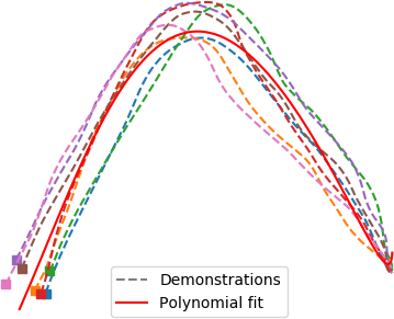
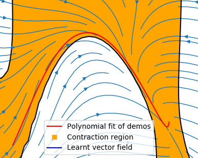
Figure 3: The figure on the left shows demonstration trajectories (dotted) and the polynomial fit of the demonstrations (solid line) for the Angle shape. The figure on the right visualizes both the polynomial fit (red), the learnt vector field (blue), and the contraction region (orange) for the incrementally stable vector field learned using our method.

Metric	DMP	SEDS	CLFDM	CVF-P
Reproduction Accuracy
TrainingTrajectoryError	4.1	7.2	4.9	6.5
TrainingVelocityError	7.4	14.6	11.0	13.9
TestTrajectoryError	5.5	4.6	12.2	3.8
TestVelocityError	8.7	11.3	15.5	11.4
Stability
DistanceToGoal	3.6	3.2	6.7	2.5
DurationToGoal	-	3.9	4.3	3.3
NumberReachedGoal	0/7	7/7	7/7	7/7
GridDuration (sec)	5.9	3.7	9.7	1.9
GridFractionReachedGoal	6%	100%	100%	100%
GridDistanceToGoal	3.3	1.0	1.0	1.0
GridDTWD ($\times 10^{4}$)	2.4	1.4	1.4	2.0
Training and Integration Speed (in seconds)
TrainingTime	0.05	2.1	2.8	0.2
IntegrationSpeed	0.21	0.06	0.15	0.01

TABLE I: LASA Angle shape benchmarks. Our approach is CVF-P.

We report in Table I comparisons on the Angle shape against state of the art methods for estimating stable dynamical systems, the Stable Estimator of Dynamical Systems (SEDS) [24], Control Lyapunov Function-based Dynamic Movements (CLFDM) [25] and Dynamic Movement Primitives (DMP) [20]. The training process in these methods involves non-convex optimization with no global optimality guarantees. Additionally, DMPs can only be trained from one demonstration one degree-of-freedom at a time. For all experiments, we learn degree 5 CVF-Ps with $\tau=1.0$ and ${\bf M}({\bf x})=\mathbf{I}$. We report the following imitation quality metrics.

Reproduction Accuracy: How well does the vector field reproduce positions and velocities in training and test demonstrations, when started from same initial conditions and integrated for the same amount of time as the human movement duration ($T$). Specifically, we measure reproduction error with respect to $m$ demonstration trajectories as,

$$\textrm{TrajectoryError}=\frac{1}{m}\sum_{i=1}^{m}\frac{1}{T_{i}}\sum_{t=0}^{T_{i}}\|{\bf x}^{i}(t)-\hat{{\bf x}}^{i}(t)\|_{2}$$

$$\textrm{VelocityError}=\frac{1}{m}\sum_{i=1}^{m}\frac{1}{T_{i}}\sum_{t=0}^{T_{i}}\|\dot{{\bf x}}^{i}(t)-\hat{\dot{{\bf x}}}^{i}(t)\|_{2}.$$

The metrics TrainingTrajectoryError, TestTrajectoryError, TrainingVelocityError, TestVelocityError report these measures with respect to training and test demonstrations. At the end of the integration duration ($T$), we also report DistanceToGoal: how far the final state is from the goal (origin). Finally, to account for the situation where the learnt dynamics is somewhat slower than the human demonstration, we also generate trajectories for a much longer time horizon ($30T$) and report ${\it DurationToGoal}$: the time it took for the state to enter a ball of radius $1mm$ around the goal, and how often this happened for the $7$ demonstrations (NumReachedGoal).

Stability: To measure stability properties, we evolve the dynamical system from $16$ random positions on a grid enclosing the demonstrations for a long integration time horizon (30T). We report the fraction of trajectories that reach the goal ($GridFraction$); the mean duration to reach the goal when that happens ($GridDuration$); the mean distance to the Goal ($GridDistanceToGoal$) and the closest proximity of the generated trajectories to a human demonstration, as measured using Dynamic Time Warping Distance ($GridDTWD$) [23] (since in this case trajectories are likely of lengths different from demonstrations).

Training and Integration Speed: We measure both training time as well as time to evaluate the dynamical system which translates to integration speed.

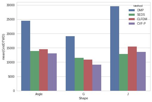
Figure 4: GridDTWD comparison on Angle, G and J shapes.

It can be seen that our approach is highly competitive on most metrics: reproduction quality, stability, and training and inference speed. In particular, it returns the best mean dynamic time warping distance to the demonstrations when initialized from points on a grid. A comparison of GridDTWD on a few other shapes is shown in Figure. 4.

V Pick-and-Place with Obstacles

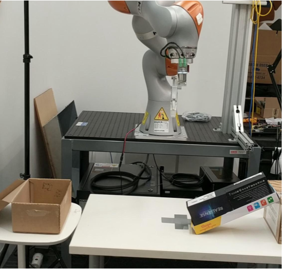
(a) Home

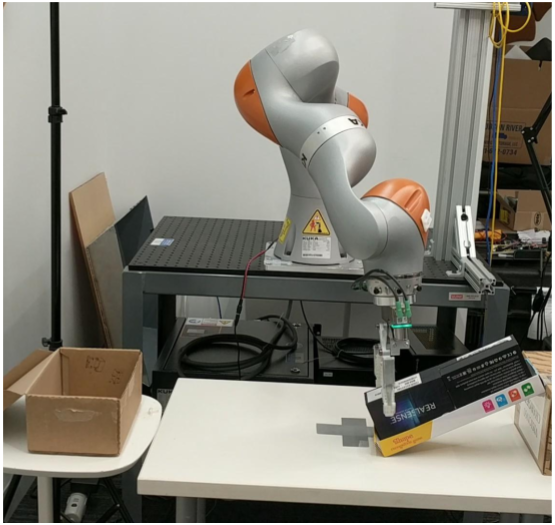
(b) Pick

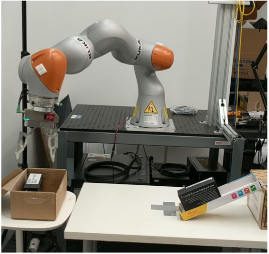
(c) Place

Figure 5: In our task, the robot must move between the (a) home to (b) pick, (c) a place positions.

We consider a kitting task shown in Figure 5 where objects are picked from a known location and placed into a box. A teleoperator quickly demonstrates a few trajectories guiding a 7DOF KUKA IIWA arm to grasp objects and place them in a box. After learning from demonstrations, the robot is expected to continually fill boxes to be verified and moved by a human working in close proximity freely moving obstacles in and out of the workspace. The arm is velocity-controlled in joint space at $50$ Hz.

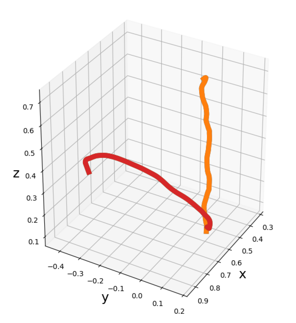
(a) Demonstration Trajectory

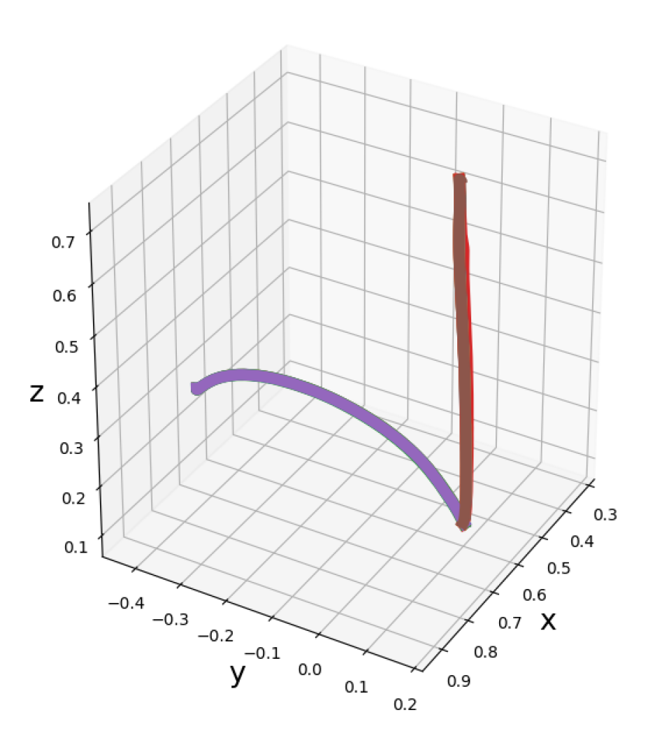
(b) CVF-P

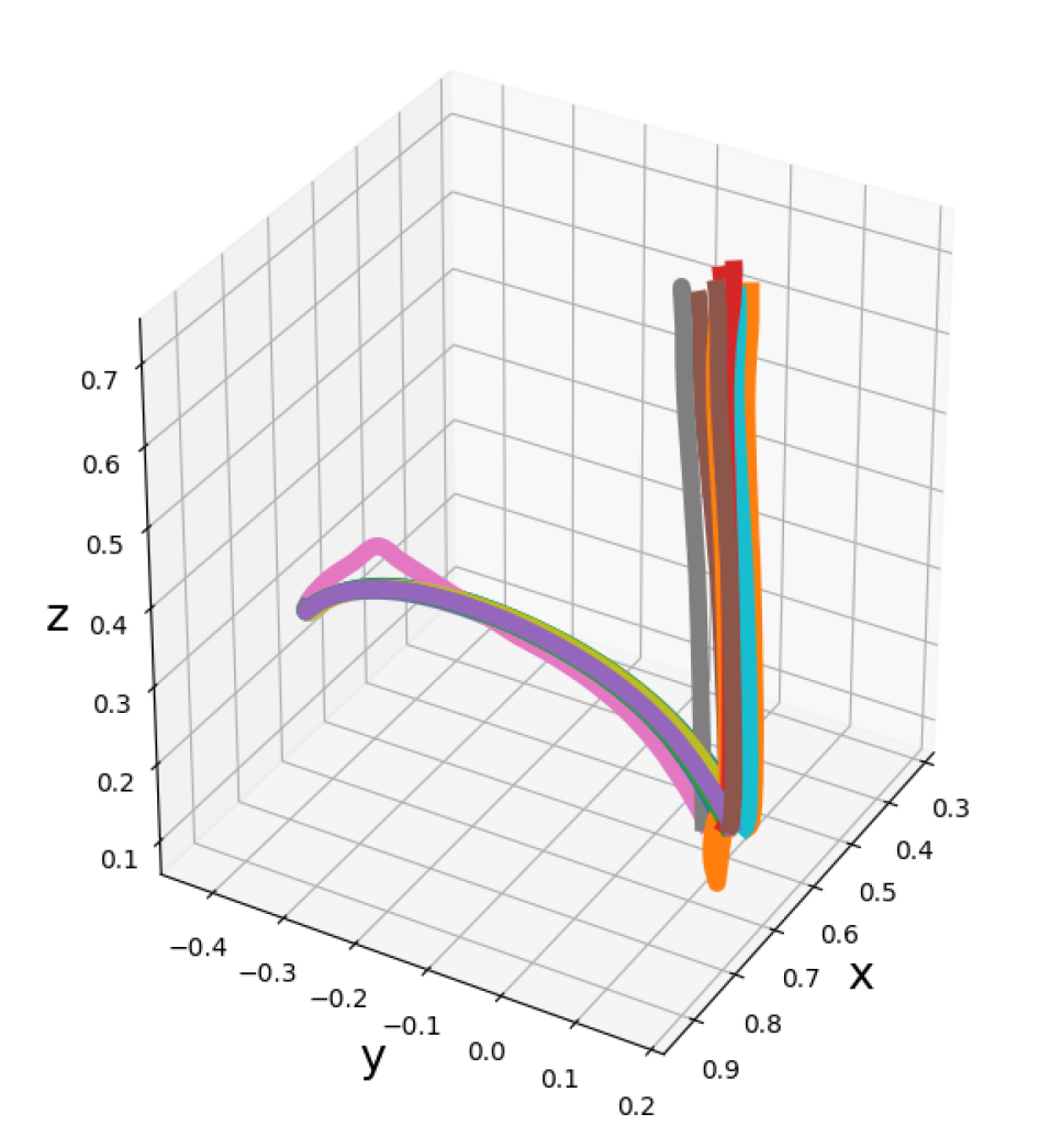
(c) CVF-P, 0.05 Noise

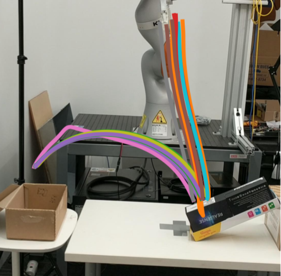
(d) CVF-P, 0.05 Noise

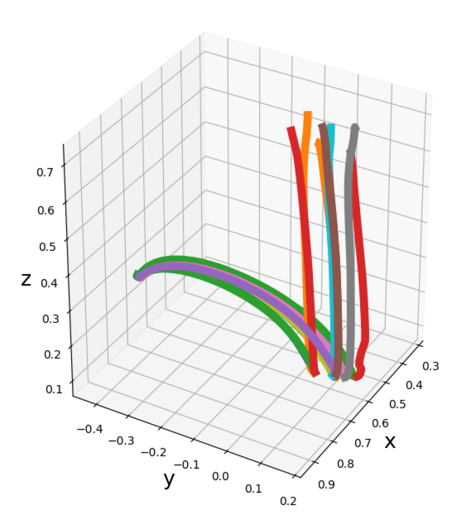
(e) CVF-P, 0.1 Noise

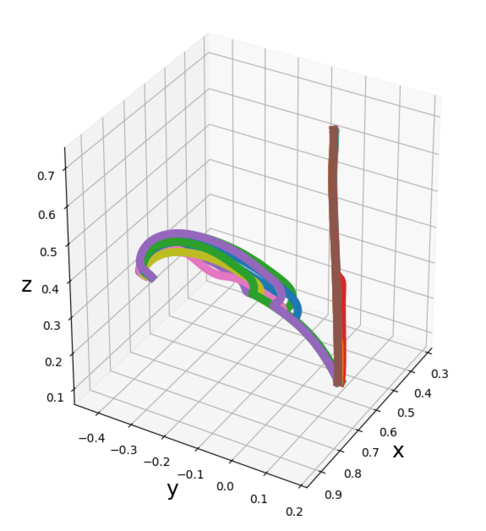
(f) CVF-P and Obstacle

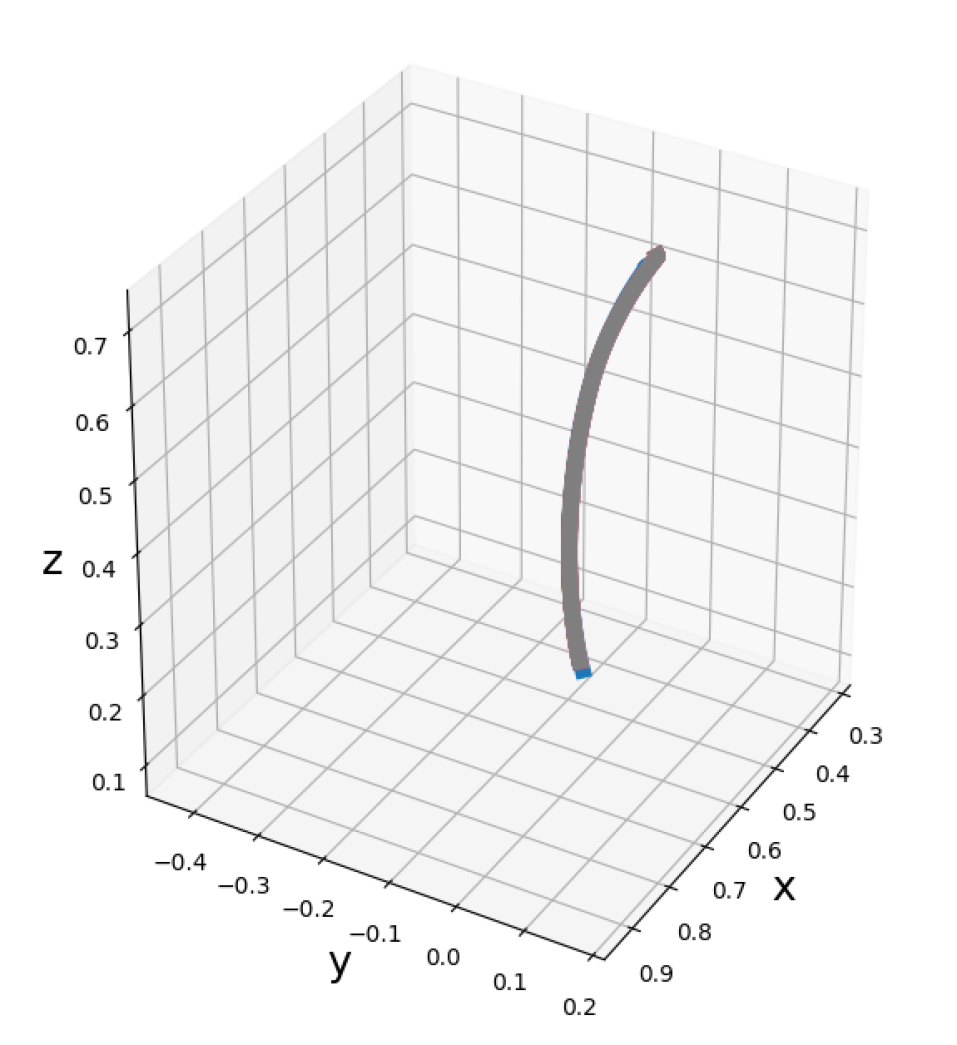
(g) VF-P, No Contraction,
No Noise, No Obstacle

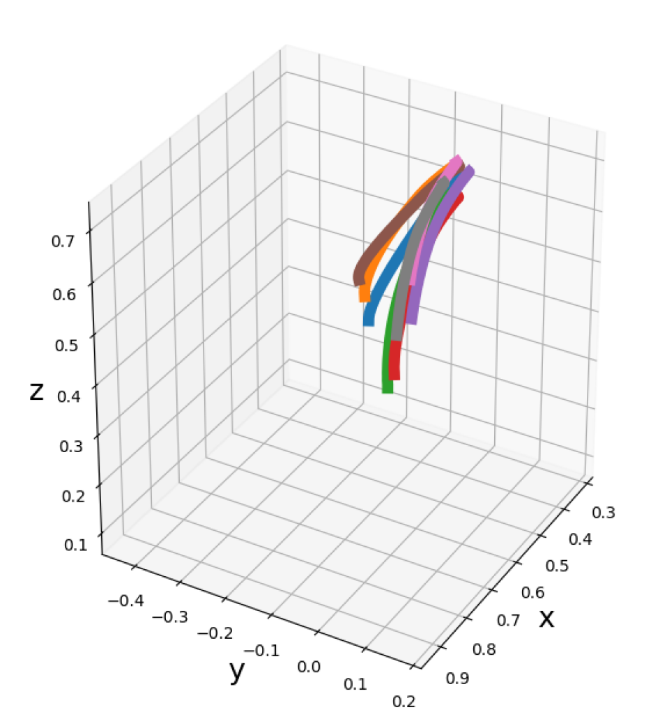
(h) VF-P, No Contraction,
0.05 Noise, No Obstacle

Figure 6: (a) A user demonstrated trajectory visualization shows the path of the end effector through cartesian space. (b) Eight trajectories executed using a vectorfield in joint space learned from the demonstration. (c,d) Eight trajectories with uniform noise between [-0.05, 0.05] radians was added per-joint to the initial joint state. (e) Eight trajectories with uniform noise between [-0.1, 0.1] added to the initial joint state. (f) Eight new trajectories with an object in the way that modulates the learned vector field. Notice the motion deviates, and then returns to the desired trajectory. (g) Eight trajectories without contraction, the arm deviates from the demonstration and cannot complete the trajectory. (h) Eight trajectories without contraction and [-0.05, 0.05] noise, the arm cannot complete the trajectory.

V-A Demonstration Trajectory

Figure 6(a) shows the demonstration pick and place trajectory collected from the user. This trajectory was collected using an HTC Vive controller operated by a user standing in front of and watching the robot move through the demonstration as it is produced. Different buttons on the remote were used to open/close the gripper, send the arm to the Home position, and indicate the start of a new trajectory. The pick and place task was collected as two separate trajectories, one for the pick motion and another for the place motion.

V-B Learning a Composition of Pick and Place CVF-Ps

Using the demonstration trajectory, two different polynomial contracting vector fields (CVF-Ps) were fit to the data, one for the pick motion, one for the place. These trajectories were fit to a degree 2 polynomial with $\tau=0.1$ and ${\bf M}({\bf x})=\mathbf{I}$, using an SCS solver run for 2500 iterations. For the ease of visualization, we show the trajectories in cartesian space in Figure 6. The CVF-P was fit to the trajectory in the 7-dimensional joint space. The arm was then run through using the vector field eight times starting from the home position. Each trajectory was allowed to run until the $L_{2}$-norm of the arm joint velocities dropped below a threshold of $0.01$. At that point, the arm would begin to move using the second vector field. The trajectories taken by the arm are shown in Figure 6(b). The eight runs have very little deviation from each other.

V-C Generalization to Different Initial Poses

Next, noise is added to the home position of the arm, and again the vector field is used to move the arm through the task. Figure 6(c) noise is added uniformly from the range [-0.05, 0.05] radians to each value of each joint of the arm’s starting home position. Figure 6(d), shows these same trajectories overlaid on the Kuka arm. In Figure 6(e) uniform noise is added in the same manner from the range $[-0.1,0.1]$. Due to contraction, trajectories are seen to converge from random initial conditions.

V-D What happens without contraction constraints?

In Figure 6(g) the arm is run eight times using a vector field without contraction. While the arm is consistent in the trajectory that it takes, the arm moves far from the demonstrated trajectory, and eventually causes the emergency break to activate at joint limits, failing to finish the task.

In Figure 6(h) The arm is again run eight times without contraction with noise added uniformly from the range [-0.05, 0.05] to each the value of each joint of the arm’s starting home position. The trajectory of the arm varies widely and had to be cut short as it was continually causing the emergency break to engage.

V-E Whole-body Obstacle Avoidance

Here we enable a Kuka robot arm to follow demonstrated trajectories while avoiding obstacles unseen during training. In the system we describe below, collisions are avoided against any part of robot body. At every timestep, a commodity depth sensor like the Intel RealSense or PhaseSpace motion capture acquires a point cloud representation of the obstacle. Our setup is along the lines of [22], although we do not model occluded regions as occupied. At this point, our demonstrations and trajectories exist in joint space $\mathcal{J}\approx\mathbb{R}^{7}$, while our obstacle pointclouds exists in Cartesian space $\mathcal{C}\approx\mathbb{R}^{3}$ with an origin at the base of the robot.

V-E1 Cartesian to Joint Space Map

We pre-compute a set-valued inverse kinematic map $\operatorname{IK}$ that maps a position $c\in\mathcal{C}$ to a subset of $\mathcal{J}$ containing all the joint configurations that would cause any part of the arm to occupy the position $c$.

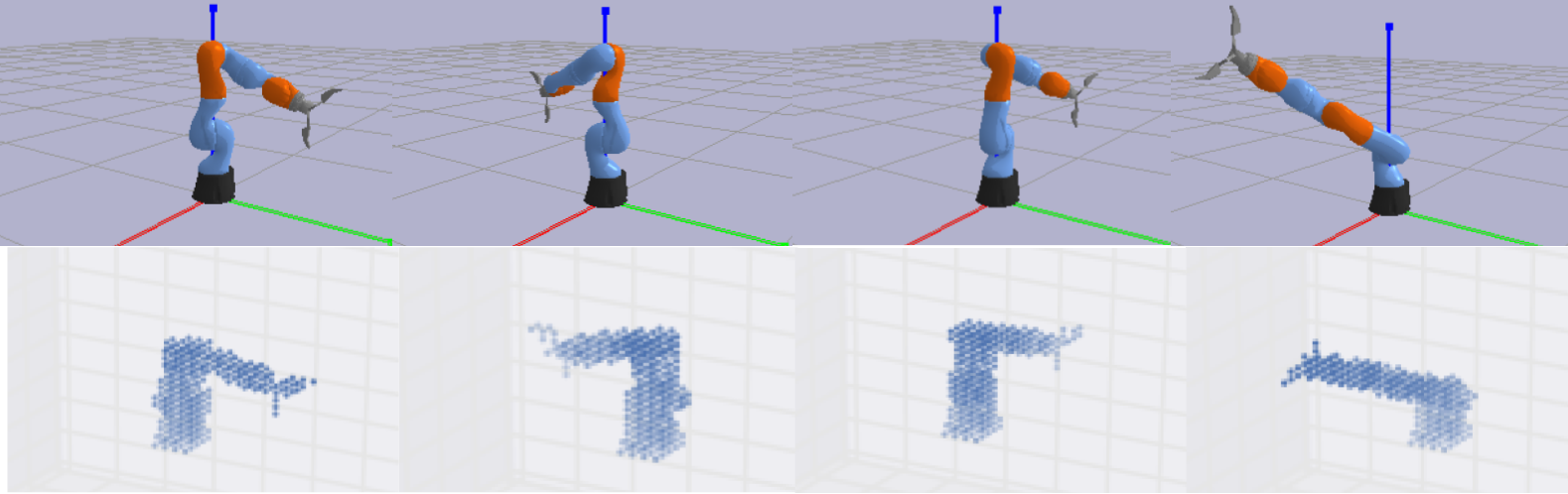
Figure 7: In order to produce a cartesian to joint space mapping, pybullet [12] was used to place the arm in over 658,945 configurations such as the 4 in the top row. Then a voxelization of the arm was produced in this pose using binvox.

More formally, the obstacles positions are known in Cartesian space $\mathcal{C}$ different from the control space $\mathcal{J}$ of the robot. (e.g. we control the joint angles rather than end-effector pose.) The Kuka arm simulator allows us to query the forward kinematics map ${\operatorname{FK}}:\mathcal{J}\rightarrow\mathcal{C}$. To compute the inverse of this map, the joint space of the robot was discretized into 658,945 discrete positions. These discrete positions were created by regularly sampling each joint from a min to max angle using a step size of 0.1 radians. As shown in Figure 7, the robot was positioned at each point of the 658,945 discrete joint space points within pybullet[12], and the robot was voxelized using binvox[35]. This produced the map ${\operatorname{FK}}$. We then compute $\operatorname{IK}\coloneqq{\operatorname{FK}}^{-1}$.

V-E2 Modulation of Contracting Vector Fields

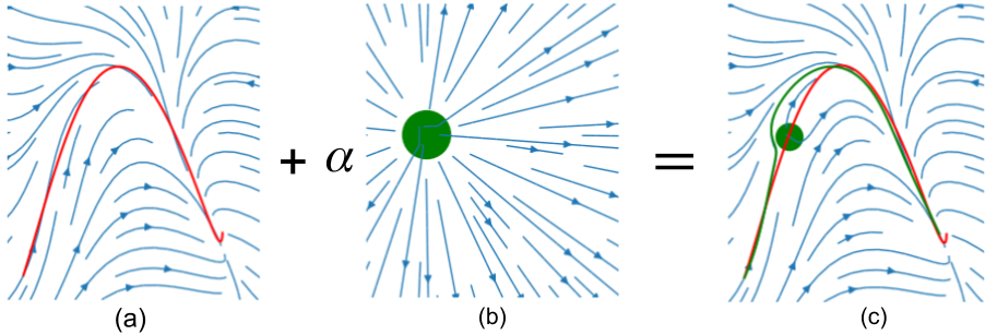
Figure 8: (a) Shows a vector field $f$ learnt from a nominal path (red). (b) Depicts a repulsive vector field $h^{\text{obstacles}}$ associated with an obstacle (green disk). (c) Shows modulated vector field $\tilde{f}$ (blue) plotted with a sample trajectory (green).

The obstacle positions are then incorporated in a repulsive vector-field to push the arm away from collision as it moves,

$$h^{\text{obstacles}}(t,{\bf x})\coloneqq\sum_{\begin{subarray}{c}\text{positions of}\\ \text{obstacles $c$}\\ \text{at time $t$}\end{subarray}}\quad\sum_{j\in T^{-1}(c)}\frac{{\bf x}-j}{\|{\bf x}-j\|_{2}^{r}},$$ (12)

where the integer $r$ control how fast the effect of this vector field decays as a function of distance (a high value of $r$ makes the effect of $h^{\text{obstacles}}$ local, while a small value makes its effect more uniform.) This vector field is added to our learnt vector-field $f$ to obtain a modulated vector field (depicted in Figure 8)

$$\tilde{f}(t,{\bf x})=f({\bf x})+\alpha\;h^{\text{obstacles}}(t,{\bf x}),$$

where $\alpha$ is positive constant that is responsible for controlling the strength of the modulation, that is then fed to the Kuka arm. If the modulation is local and the obstacle is well within the joint-space contraction tube, we expect the motion to re-converge to the demonstrated behavior.

We point out that it is possible to use alternative modulation methods that come with different guarantees and drawbacks. In [26, 19] for instance, the authors use a multiplicative modulation function that preserves equilibrium points in the case of convex or concave obstacles.

While our approach does not enjoy the same guarantees, its additive nature allows us to handle a large number of obstacles as every term in Eqn. 12 can be computed in a distributed fashion, and furthermore, we do not need to impose any restrictions on the shape of the obstacles (convex/concave). This is particularly important as our control space $\mathcal{J}$ is different from the space $\mathcal{C}$ where the obstacle are observed, and the map $\operatorname{IK}$ that links between the two spaces can significantly alter the shape of an obstacle in general (e.g. a sphere in cartesian space can be mapped to a disconnected set in joint space).

V-E3 Real-time Obstacle Avoidance

Here, using a real-time motion capture system, an obstacle is introduced to the robot’s workspace as shown in Figure 1(b). Eight trajectories were executed from the home position with the obstacle in the workspace, and the resultant trajectories are shown in Figure 6(f). At each timestep, the objects position was returned by the motion capture system. The point in Cartesian space was used to modulate the joint space vectorfield as described in Section V-E. The tasks are accomplished as the arm avoids obstacles but remains within the joint-space contraction tube re-converging to the demonstrated behavior.

VI Conclusion

This work presents a novel approach to teleoperator imitation using contracting vector fields that are globally optimal with respect to loss minimization and providing continuous-time guarantees on the behaviour of the system when started from within a contraction tube around the demonstration. Our approach compares favorably with other movement generation techniques. Additionally, we build a workspace cartesian to joint space map for the robot, and utilize it to update our CVF on the fly to avoid dynamic obstacles. We demonstrate how this approach enables the transfer of knowledge from humans to robots for accomplishing a real world robotic pick and place task. Future work includes greater scalability of our solution, composition of CVFs for more complex tasks, integrating with a perception module and helping bootstrap data-hungry reinforcement learning approaches.

References

- [1] https://cs.stanford.edu/people/khansari/download.html.
- [2] Amir Ali Ahmadi. Algebraic relaxations and hardness results in polynomial optimization and lyapunov analysis. arXiv preprint arXiv:1201.2892, 2012.
- [3] Amir Ali Ahmadi and Bachir El Khadir. Time-varying semidefinite programs. arXiv preprint arXiv:1808.03994, 2018.
- [4] Amir Ali Ahmadi, Georgina Hall, Ameesh Makadia, and Vikas Sindhwani. Geometry of 3d environments and sum of squares polynomials. arXiv preprint arXiv:1611.07369, 2016.
- [5] Amir Ali Ahmadi and Anirudha Majumdar. Dsos and sdsos optimization: Lp and socp-based alternatives to sum of squares optimization. In 2014 48th annual conference on information sciences and systems (CISS), pages 1–5. IEEE, 2014.
- [6] Amir Ali Ahmadi and Pablo A Parrilo. Towards scalable algorithms with formal guarantees for lyapunov analysis of control systems via algebraic optimization. In 2014 IEEE 53rd Annual Conference on Decision and Control (CDC), pages 2272–2281. IEEE, 2014.
- [7] Christopher G Atkeson, BPW Babu, N Banerjee, D Berenson, CP Bove, X Cui, M DeDonato, R Du, S Feng, P Franklin, et al. What happened at the darpa robotics challenge, and why.
- [8] Erin M Aylward, Pablo A Parrilo, and Jean-Jacques E Slotine. Stability and robustness analysis of nonlinear systems via contraction metrics and sos programming. Automatica, 44(8):2163–2170, 2008.
- [9] Aude Billard, Sylvain Calinon, Ruediger Dillmann, and Stefan Schaal. Robot programming by demonstration. In Springer handbook of robotics, pages 1371–1394. Springer, 2008.
- [10] Man-Duen Choi. Positive semidefinite biquadratic forms. Linear Algebra and its Applications, 12(2):95–100, 1975.
- [11] Man-Duen Choi, Tsit-Yuen Lam, and Bruce Reznick. Real zeros of positive semidefinite forms. I. Mathematische Zeitschrift, 171(1):1–26, 1980.
- [12] Erwin Coumans and Yunfei Bai. pybullet, a python module for physics simulation, games, robotics and machine learning. http://pybullet.org/, 2016–2017.
- [13] Hongkai Dai, Anirudha Majumdar, and Russ Tedrake. Synthesis and optimization of force closure grasps via sequential semidefinite programming. In Robotics Research, pages 285–305. Springer, 2018.
- [14] Holger Dette and William J. Studden. Matrix measures, moment spaces and Favard’s theorem for the interval [0,1] and [0, ). Linear Algebra and its Applications, 345(1-3):169–193, April 2002.
- [15] Anca D Dragan and Siddhartha S Srinivasa. Formalizing assistive teleoperation. MIT Press, 2012.
- [16] Terrence Fong and Charles Thorpe. Vehicle teleoperation interfaces. Autonomous robots, 11(1):9–18, 2001.
- [17] Karin Gatermann and Pablo A Parrilo. Symmetry groups, semidefinite programs, and sums of squares. Journal of Pure and Applied Algebra, 192(1-3):95–128, 2004.
- [18] Ken Goldberg, Michael Mascha, Steve Gentner, Nick Rothenberg, Carl Sutter, and Jeff Wiegley. Desktop teleoperation via the world wide web. In Robotics and Automation, 1995. Proceedings., 1995 IEEE International Conference on, volume 1, pages 654–659. IEEE, 1995.
- [19] Lukas Huber, Aude Billard, and Jean-Jacques E. Slotine. Avoidance of convex and concave obstacles with convergence ensured through contraction. IEEE Robotics and Automation Letters, PP:1–1, 01 2019.
- [20] Auke Jan Ijspeert, Jun Nakanishi, Heiko Hoffmann, Peter Pastor, and Stefan Schaal. Dynamical movement primitives: learning attractor models for motor behaviors. Neural computation, 25(2):328–373, 2013.
- [21] Jerome Jouffroy and Thor I Fossen. A tutorial on incremental stability analysis using contraction theory. Modeling, Identification and control, 31(3):93, 2010.
- [22] Daniel Kappler, Franziska Meier, Jan Issac, Jim Mainprice, Cristina Garcia Cifuentes, Manuel Wüthrich, Vincent Berenz, Stefan Schaal, Nathan Ratliff, and Jeannette Bohg. Real-time perception meets reactive motion generation. IEEE Robotics and Automation Letters, 3(3):1864–1871, 2018.
- [23] Eamonn Keogh and Chotirat Ann Ratanamahatana. Exact indexing of dynamic time warping. Knowledge and information systems, 7(3):358–386, 2005.
- [24] S Mohammad Khansari-Zadeh and Aude Billard. Learning stable nonlinear dynamical systems with gaussian mixture models. IEEE Transactions on Robotics, 27(5):943–957, 2011.
- [25] S. Mohammad Khansari-Zadeh and Aude Billard. Learning control lyapunov function to ensure stability of dynamical system-based robot reaching motions. Robotics and Autonomous Systems, 6(62), 2014.
- [26] Seyed Mohammad Khansari-Zadeh and Aude Billard. A dynamical system approach to realtime obstacle avoidance. Autonomous Robots, 32(4):433–454, 2012.
- [27] Seyed Mohammad Khansari-Zadeh and Oussama Khatib. Learning potential functions from human demonstrations with encapsulated dynamic and compliant behaviors. Autonomous Robots, 41(1):45–69, 2017.
- [28] Oussama Khatib. Real-time obstacle avoidance for manipulators and mobile robots. The international journal of robotics research, 5(1):90–98, 1986.
- [29] Masakazu Kojima. Sums of squares relaxations of polynomial semidefinite programs. Research report B-397, Dept. of Mathematical and Computing Sciences, Tokyo Institute of Technology, 2003.
- [30] J. B. Lasserre. Global optimization with polynomials and the problem of moments. SIAM Journal on Optimization, 11(3):796–817, January 2001.
- [31] Andre Lemme, Yaron Meirovitch, Seyed Mohammad Khansari-Zadeh, Tamar Flash, Aude Billard, and Jochen J Steil. Open-source benchmarking for learned reaching motion generation in robotics. 2015.
- [32] Winfried Lohmiller and Jean-Jacques E Slotine. On contraction analysis for non-linear systems. Automatica, 34(6):683–696, 1998.
- [33] Anirudha Majumdar, Amir Ali Ahmadi, and Russ Tedrake. Control design along trajectories with sums of squares programming. In 2013 IEEE International Conference on Robotics and Automation, pages 4054–4061. IEEE, 2013.
- [34] Naresh Marturi, Alireza Rastegarpanah, Chie Takahashi, Maxime Adjigble, Rustam Stolkin, Sebastian Zurek, Marek Kopicki, Mohammed Talha, Jeffrey A Kuo, and Yasemin Bekiroglu. Towards advanced robotic manipulation for nuclear decommissioning: a pilot study on tele-operation and autonomy. In Robotics and Automation for Humanitarian Applications (RAHA), 2016 International Conference on, pages 1–8. IEEE, 2016.
- [35] Patrick Min. Binvox, a 3d mesh voxelizer, 2004.
- [36] B. O’Donoghue, E. Chu, N. Parikh, and S. Boyd. Conic optimization via operator splitting and homogeneous self-dual embedding. Journal of Optimization Theory and Applications, 169(3):1042–1068, June 2016.
- [37] Pablo A. Parrilo. Semidefinite programming relaxations for semialgebraic problems. Mathematical Programming, 96(2):293–320, 2003.
- [38] Edouard Pauwels, Didier Henrion, and Jean-Bernard Bernard Lasserre. Inverse optimal control with polynomial optimization. arXiv preprint arXiv:1403.5180, 2014.
- [39] Michael Posa, Twan Koolen, and Russ Tedrake. Balancing and step recovery capturability via sums-of-squares optimization. In Robotics: Science and Systems, pages 12–16, 2017.
- [40] Harish Ravichandar, Iman Salehi, and Ashwin Dani. Learning partially contracting dynamical systems from demonstrations. In Conference on Robot Learning (CoRL), 2017.
- [41] Stefan Schaal. Is imitation learning the route to humanoid robots? Trends in cognitive sciences, 3(6):233–242, 1999.
- [42] Carsten W Scherer and Camile WJ Hol. Matrix sum-of-squares relaxations for robust semi-definite programs. Mathematical programming, 107(1-2):189–211, 2006.
- [43] Vikas Sindhwani, Stephen Tu, and Mohi Khansari. Learning contracting vector fields for stable imitation learning. arXiv preprint arXiv:1804.04878, 2018.
- [44] Mark Talamini, Kurtis Campbell, and Cathy Stanfield. Robotic gastrointestinal surgery: early experience and system description. Journal of laparoendoscopic & advanced surgical techniques, 12(4):225–232, 2002.
- [45] Russell H Taylor, Arianna Menciassi, Gabor Fichtinger, Paolo Fiorini, and Paolo Dario. Medical robotics and computer-integrated surgery. In Springer handbook of robotics, pages 1657–1684. Springer, 2016.
- [46] Richard Washington, Keith Golden, John Bresina, David E Smith, Corin Anderson, and Trey Smith. Autonomous rovers for mars exploration. In Aerospace Conference, 1999. Proceedings. 1999 IEEE, volume 1, pages 237–251. IEEE, 1999.
- [47] Tianhao Zhang, Zoe McCarthy, Owen Jowl, Dennis Lee, Xi Chen, Ken Goldberg, and Pieter Abbeel. Deep imitation learning for complex manipulation tasks from virtual reality teleoperation. In 2018 IEEE International Conference on Robotics and Automation (ICRA), pages 1–8. IEEE, 2018.