Short-time expansion of Heisenberg operators in open collective quantum spin systems

Abstract

We present an efficient method to compute short-time expectation values in large collective spin systems with typical forms of Markovian decoherence. Our method is based on a Taylor expansion of a formal solution to the equations of motion for Heisenberg operators. This expansion can be truncated at finite order to obtain virtually exact results at short times that are relevant for metrological applications such as spin squeezing. In order to evaluate the expansion for Heisenberg operators, we compute the relevant structure constants of a collective spin operator algebra. We demonstrate the utility of our method by computing spin squeezing, two-time correlation functions, and out-of-time-ordered correlators for $10^{4}$ spins in strong-decoherence regimes that are otherwise inaccessible via existing numerical methods. Our method can be straightforwardly generalized to the case of a collective spin coupled to bosonic modes, relevant for trapped ion and cavity QED experiments, and may be used to investigate short-time signatures of quantum chaos and information scrambling.

I Introduction

Collective spin systems are a versatile resource in quantum science for a range of applications including quantum-enhanced metrology and quantum simulation. The study of such systems dates back to the mid-twentieth century with the introduction of the Dicke modelDicke (1954) that describes atoms cooperatively interacting with a single mode of a radiation field, and the Lipkin-Meshkov-Glick (LMG) model, a toy model for testing many-body approximation methods in contemporary nuclear physicsLipkin et al. (1965); Meshkov et al. (1965); Glick et al. (1965). On the experimental side, the development of advanced trapping, cooling, and control techniques in atomic, molecular, and optical (AMO) systems have enabled the realization of collective spin models in a broad range of platforms, including cold atomic gassesTakano et al. (2009); Appel et al. (2009), Bose-Einstein condensatesKlinder et al. (2015); Estève et al. (2008); Riedel et al. (2010); Gross et al. (2010), ultracold Fermi gassesMartin et al. (2013); Bromley et al. (2018); Smale et al. (2019), trapped ionsBohnet et al. (2016), and optical cavitiesSchleier-Smith et al. (2010a); Chen et al. (2011); Baumann et al. (2010); Leroux et al. (2010); Bohnet et al. (2014); Cox et al. (2016); Hosten et al. (2016a, b); Norcia et al. (2018); Ritsch et al. (2013), among others. These implementations compliment innumerable theoretical studies in a variety of rich subjects, including quantum phase transitions and criticalityLatorre et al. (2005); Alcalde et al. (2007); Wang et al. (2012); Majd et al. (2014), non-equilibrium phenomenaWalls et al. (1978); Morrison and Parkins (2008a, b, c); Kessler et al. (2012); Bhattacherjee (2014); Zhiqiang et al. (2017); Lang et al. (2018), and precision mentrologyWineland et al. (1992); Kitagawa and Ueda (1993); Zhong (2010); Schleier-Smith et al. (2010b); Ma et al. (2011); Huang et al. (2015a); Muessel et al. (2015); Huang et al. (2015b); Hu et al. (2017); Mirkhalaf et al. (2018); Lewis-Swan et al. (2018); He et al. (2019).

One of the primary motivations for studying collective spin systems is their application to quantum-enhanced metrology. Quantum projection noise limits the error $\Delta\phi$ in the measurement of a phase angle $\phi$ with $N$ independent spins to $\Delta\phi\sim 1/\sqrt{N}$Wineland et al. (1992); Itano et al. (1993). Collective spin systems provide a means to break through this limit via the preparation of many-body entangled states such as spin-cat statesAgarwal et al. (1997); Lau et al. (2014); Huang et al. (2015b) and most notably spin-squeezed statesWineland et al. (1992); Kitagawa and Ueda (1993); Ma et al. (2011) that allow for measurement errors $\Delta\phi\sim 1/N^{\varepsilon}$ with $1/2<\varepsilon\leq 1$, where $\varepsilon=1$ saturates the Heisenberg limitZwierz et al. (2010). Such entangled states can be prepared either via heralded methods such as quantum nondemolition measurementsTakano et al. (2009); Appel et al. (2009); Schleier-Smith et al. (2010a); Chen et al. (2011), or via deterministic methods that require nonlinear dynamics, typically realized with phonon-mediatedBohnet et al. (2016), photon-mediatedKlinder et al. (2015); Baumann et al. (2010); Leroux et al. (2010); Bohnet et al. (2014); Cox et al. (2016); Hosten et al. (2016a, b); Norcia et al. (2018); Ritsch et al. (2013) or collisionalEstève et al. (2008); Riedel et al. (2010); Gross et al. (2010); Martin et al. (2013); Bromley et al. (2018); Smale et al. (2019) interactions. Although a truly collective spin model requires uniform, all-to-all interactions, as long as measurements do not distinguish between constituent particles, even non-uniform systems may be effectively described by a uniform model with renormalized parametersHu et al. (2015).

In the absence of decoherence, permutation symmetry and total spin conservation divide the total Hilbert space of a collective spin system into superselection sectors that grow only linearly with system size $N$, thereby admitting efficient classical simulation of its dynamics. Decoherence generally violates total spin conservation and requires the use of density operators, increasing the dimension of accessible state space to $O\left(N^{3}\right)$Hartmann (2016); Xu et al. (2013). In this case, exact simulations can be carried out for $N\lesssim 100$ particles. If decoherence is sufficiently weak, dynamics can be numerically solvable for $N\lesssim 10^{5}$ particles via “quantum trajectory” Monte Carlo methodsPlenio and Knight (1998); Zhang et al. (2018) (also known as “quantum jump” or “Monte Carlo wavefunction” methods) that can reproduce all expectation values of interest. When decoherence is strong, however, these Monte Carlo methods can take a prohibitively long time to converge, as simulations become dominated by incoherent jumps that generate large numbers of distinct quantum trajectories that need to be averaged in order to accurately compute expectation values. Even with strong decoherence, dynamics are sometimes solvable through the cumulant expansionMeiser and Holland (2010) that neglects all $n$-body connected correlators for $n>2$. The growth of genuinely multi-body correlations, however, eventually causes the cumulant expansion to yield incorrect results with no clear signature of failure. In the absence of other means to compute correlators, it can therefore be difficult to identify the point at which correlators computed via the cumulant expansion can no longer be trusted.

In this work, we present an efficient method to compute short-time dynamics of collective spin systems with typical forms of Markovian decoherence. The only restriction on decoherence (beyond Markovianity) is that, like the coherent collective dynamics, it must act identically on all constituent particles. Our method is based on a formal solution to the equations of motion for Heisenberg operators, thereby bearing some resemblance to the Mori formalismMori (1965) and related workAnnett et al. (1994). Specifically, we expand a formal solution for a Heisenberg operator into a Taylor series whose truncation can yield negligible error at sufficiently short times. Evaluating the resulting expansion requires knowing the structure constants of a collective spin operator algebra; the calculation of these structure constants (in Appendices A–C) is one of the main technical results of this work, which we hope will empower both analytical and numerical studies of collective spin systems in the future. We benchmark our method against exact results from both analytical calculations and quantum trajectory Monte Carlo computations of spin squeezing in accessible parameter regimes, highlighting both advantages and limitations of the short-time expansion. Finally, we showcase applications of our method by computing quantities that are inaccessible to other numerical methods.

II Theory

In this section we provide the basic theory for our method to compute expectation values of collective spin operators, deferring lengthy derivations to the appendices. We consider a system of $N$ distinct spin-1/2 particles. Defining individual spin-1/2 operators $\hat{s}_{\alpha=\text{x},\text{y},\text{z}}\equiv\hat{\sigma}_{\alpha}/2$ and $\hat{s}_{\pm}\equiv\hat{s}_{\text{x}}\pm i\hat{s}_{\text{y}}=\hat{\sigma}_{\pm}$ with Pauli operators $\hat{\sigma}_{\alpha}$, we denote an operator that acts with $\hat{s}_{\alpha}$ on the spin indexed by $j$ and trivially (i.e. with the identity $\hat{\mathds{1}}$) on all other spins by $\hat{s}_{\alpha}^{(j)}$. We then define the collective spin operators $\hat{S}_{\alpha}\equiv\sum_{j=1}^{N}\hat{s}_{\alpha}^{(j)}$ for $\alpha\in\set{\text{x},\text{y},\text{z},+,-}$. Identifying the set $\set{\hat{\mathcal{S}}_{\bm{m}}}$ as a basis for all collective spin operators, with $\bm{m}\equiv\left(m_{+},m_{\text{z}},m_{-}\right)\in\mathbb{N}_{0}^{3}$ and $\hat{\mathcal{S}}_{\bm{m}}\equiv\hat{S}_{+}^{m_{+}}\hat{S}_{\text{z}}^{m_{\text{z}}}\hat{S}_{-}^{m_{-}}$, we can expand any collective spin operator $\hat{\mathcal{O}}$ in the form

$$\hat{\mathcal{O}}=\sum_{\bm{m}}\mathcal{O}_{\bm{m}}\hat{\mathcal{S}}_{\bm{m}}$$ (1)

with scalar coefficients $\mathcal{O}_{\bm{m}}\in\mathbb{C}$. If $\hat{\mathcal{O}}$ is self-adjoint, for example, then $\mathcal{O}_{\bm{m}}^{*}=\mathcal{O}_{\bm{m}^{*}}$ with $\bm{m}^{*}\equiv\left(m_{-},m_{\text{z}},m_{+}\right)$. The corresponding Heisenberg operator is then $\hat{\mathcal{O}}\left(t\right)=\sum_{\bm{m}}\mathcal{O}_{\bm{m}}\left(t\right)\hat{\mathcal{S}}_{\bm{m}}+\hat{\mathcal{E}}_{\mathcal{O}}\left(t\right)$, with time-dependent coefficients $\mathcal{O}_{\bm{m}}\left(t\right)$ for time-independent Schrödinger operators $\hat{\mathcal{S}}_{\bm{m}}$, and mean-zero “noise” operators $\hat{\mathcal{E}}_{\mathcal{O}}\left(t\right)$ that result from interactions between the spin system and its environment, initially $\hat{\mathcal{E}}_{\mathcal{O}}\left(0\right)=0$. These noise operators will essentially play no role in the present work, but are necessary to include for a consistent formalism of Heisenberg operators in an open quantum system; see Appendix N for further discussion. The expectation values of Heisenberg operators evolve according to

$$\dfrac{d}{dt}\braket{\hat{\mathcal{O}}\left(t\right)}=\braket{\check{T}\hat{\mathcal{O}}\left(t\right)}=\sum_{\bm{m},\bm{n}}\braket{\hat{\mathcal{S}}_{\bm{m}}}T_{\bm{m}\bm{n}}\mathcal{O}_{\bm{n}}\left(t\right)$$ (2)

with a Heisenberg-picture time derivative operator $\check{T}=d/dt$ whose matrix elements $T_{\bm{m}\bm{n}}\in\mathbb{C}$ are defined by

$$\check{T}\hat{\mathcal{S}}_{\bm{n}}\equiv i\left[\hat{H},\hat{\mathcal{S}}_{\bm{n}}\right]_{-}+\sum_{\mathcal{J}}\gamma_{\mathcal{J}}\check{\mathcal{D}}\left(\mathcal{J}\right)\hat{\mathcal{S}}_{\bm{n}}=\sum_{\bm{m}}\hat{\mathcal{S}}_{\bm{m}}T_{\bm{m}\bm{n}},$$ (3)

where $\left[X,Y\right]_{\pm}\equiv XY\pm YX$; $\hat{H}$ is the collective spin Hamiltonian; $\mathcal{J}$ is a set of jump operators with a corresponding decoherence rate $\gamma_{\mathcal{J}}$; and $\check{\mathcal{D}}$ is a Heisenberg-picture dissipator, or Lindblad superoperator, defined by

$$\check{\mathcal{D}}\left(\mathcal{J}\right)\hat{\mathcal{O}}\equiv\sum_{\hat{J}\in\mathcal{J}}\left(\hat{J}^{\dagger}\hat{\mathcal{O}}\hat{J}-\dfrac{1}{2}\left[\hat{J}^{\dagger}\hat{J},\hat{\mathcal{O}}\right]_{+}\right).$$ (4)

Decoherence via uncorrelated decay of individual spins, for example, would be described by the set of jump operators $\mathcal{J}_{-}\equiv\set{\hat{s}_{-}^{(j)}\mathrel{\mathop{\mathchar 58\relax}}j=1,2,\cdots,N}$. The commutator in Eq. (3) can be computed by expanding the product $\hat{\mathcal{S}}_{\bm{\ell}}\hat{\mathcal{S}}_{\bm{m}}=\sum_{\bm{n}}f_{\bm{\ell}\bm{m}\bm{n}}\hat{\mathcal{S}}_{\bm{n}}$ with structure constants $f_{\bm{\ell}\bm{m}\bm{n}}\in\mathbb{R}$ that we work out in Appendices A–C, and the effects of decoherence from jump operators (i.e. elements of $\mathcal{J}$) of the form $\hat{g}^{(j)}=\sum_{\alpha}g_{\alpha}\hat{s}_{\alpha}^{(j)}$ and $\hat{G}=\sum_{\alpha}G_{\alpha}\hat{S}_{\alpha}$ are worked out in Appendices D–G. We consider these calculations to be some of the main technical contributions of this work, with potential applications beyond the short-time simulation method presented here. These ingredients are sufficient to compute matrix elements $T_{\bm{m}\bm{n}}$ of the time derivative operator $\check{T}$ in Eq. (3) in most cases of practical interest.

We note that particle loss is an important decoherence mechanism in many experimental realizations of collective spin modelsMa et al. (2011). In principle, a spin model has no notion of the particle annihilation operators that generate particle loss, and therefore cannot capture this effect directly. Nonetheless, for a system initially composed of $N$ particles, the effect of particle loss can be emulated with $O(1/N)$ error by the dissipator $\check{\mathcal{D}}_{\text{loss}}$ defined by $\check{\mathcal{D}}_{\text{loss}}\hat{\mathcal{S}}_{\bm{m}}=-\lvert\bm{m}\rvert\hat{\mathcal{S}}_{\bm{m}}$, where $\lvert\bm{m}\rvert\equiv\sum_{\alpha}m_{\alpha}$ (see Appendix H). Furthermore, the effect particle loss can be accounted for exactly by 1. introducing an additional index on spin operators, $\hat{\mathcal{S}}_{\bm{m}}\to\hat{\mathcal{S}}_{N\bm{m}}$, to keep track of different sectors of fixed particle number within a multi-particle Fock space, and 2. constructing jump operators that appropriately couple spin operators within different particle-number sectors. We defer a detailed exact accounting of particle loss to future work.

The time derivative operator $\check{T}$ will generally couple spin operators $\hat{\mathcal{S}}_{\bm{n}}$ to spin operators $\hat{\mathcal{S}}_{\bm{m}}$ with higher “weight”, i.e. with $\lvert\bm{m}\rvert>\lvert\bm{n}\rvert$. The growth of operator weight signifies the growth of many-body correlations. Keeping track of this growth eventually becomes intractable, requiring us to truncate our equations of motion somehow. The simplest truncation strategy would be to take

$$\dfrac{d}{dt}\braket{\hat{\mathcal{O}}\left(t\right)}\to\sum_{w\left(\bm{m}\right)<W}\braket{\hat{\mathcal{S}}_{\bm{m}}}\sum_{\bm{n}}T_{\bm{m}\bm{n}}\mathcal{O}_{\bm{n}}\left(t\right)$$ (5)

for some weight measure $w$, e.g. $w\left(\bm{m}\right)=\lvert\bm{m}\rvert$, and a high-weight cutoff $W$. The truncation in Eq. (5) closes the system of differential equations defined by Eq. (2), and allows us to solve it using standard numerical methods. Some initial conditions for this system of differential equations, namely expectation values of collective spin operators with respect to spin-polarized (Gaussian) states that are generally simple to prepare experimentally, are provided in Appendix I.

The truncation strategy in Eq. (5) has a few limitations: 1. simulating a system of differential equations for a large number of operators can be time-consuming, 2. the weight measure $w$ may need to be chosen carefully, as the optimal measure is generally system-dependent, and 3. simulation results can only be trusted up to the time at which the initial values of operators $\hat{\mathcal{S}}_{\bm{m}}$ with weight $w\left(\bm{m}\right)\geq W$ have a non-negligible contribution to expectation values of interest. The last limitation in particular unavoidably applies in some form to any method tracking only a subset of all relevant operators. We therefore devise an alternate truncation strategy built around limitation 3.

We can formally expand Heisenberg operators $\hat{\mathcal{O}}\left(t\right)$ in a Taylor series about the time $t=0$ to write

$$\braket{\hat{\mathcal{O}}\left(t\right)}=\braket{e^{t\check{T}}\hat{\mathcal{O}}\left(0\right)}=\sum_{k\geq 0}\dfrac{t^{k}}{k!}\sum_{\bm{m},\bm{n}}\braket{\hat{\mathcal{S}}_{\bm{m}}}T^{k}_{\bm{m}\bm{n}}\mathcal{O}_{\bm{n}}\left(0\right),$$ (6)

where the matrix elements $T^{k}_{\bm{m}\bm{n}}$ of the $k$-th time derivative operator $\check{T}^{k}$ are

$$T^{0}_{\bm{m}\bm{n}} \equiv\delta_{\bm{m}\bm{n}},$$ (7)

$$T^{1}_{\bm{m}\bm{n}} \equiv T_{\bm{m}\bm{n}},$$ (8)

$$T^{k>1}_{\bm{m}\bm{n}} \equiv\sum_{\bm{p}_{1},\bm{p}_{2},\cdots,\bm{p}_{k-1}}T_{\bm{m}\bm{p}_{k-1}}\cdots T_{\bm{p}_{3}\bm{p}_{2}}T_{\bm{p}_{2}\bm{p}_{1}}T_{\bm{p}_{1}\bm{n}},$$ (9)

with $\delta_{\bm{m}\bm{n}}=1$ if $\bm{m}=\bm{n}$ and zero otherwise. For sufficiently short times, we can truncate the series in Eq. (6) by taking

$$\braket{\hat{\mathcal{O}}\left(t\right)}\to\sum_{k=0}^{M}\dfrac{t^{k}}{k!}\sum_{\bm{m},\bm{n}}\braket{\hat{\mathcal{S}}_{\bm{m}}}T^{k}_{\bm{m}\bm{n}}\mathcal{O}_{\bm{n}}\left(0\right).$$ (10)

We refer to Eq. (10) as the truncated short-time (TST) expansion of Heisenberg operators. Note that when computing an expectation value $\braket{\hat{\mathcal{O}}\left(t\right)}$, the relation $\hat{\mathcal{S}}_{\bm{m}}^{\dagger}=\hat{\mathcal{S}}_{\bm{m}^{*}}$, which by Hermitian conjugation of Eq. (2) also implies that $T_{\bm{m}^{*}\bm{n}^{*}}=T_{\bm{m}\bm{n}}^{*}$, cuts both the number of initial-time expectation values $\braket{\hat{\mathcal{S}}_{\bm{m}}}$ and the number of matrix elements $T_{\bm{m}\bm{n}}$ that we may need to explicitly compute roughly in half.

Unlike the weight-based truncation in Eq. (5), the nonzero matrix elements $T^{k}_{\bm{m}\bm{n}}$ for $k=0,1,\cdots,M$ in Eq. (10) tell us which operators $\hat{\mathcal{S}}_{\bm{m}}$ are relevant for computing the expectation value $\braket{\hat{\mathcal{O}}\left(t\right)}$ to a fixed order $M$. The TST expansion thereby avoids the introduction of a weight measure $w$ that chooses which operators to keep track of, and trades the cost of solving a system of differential equations for the cost of computing expectation values $\braket{\hat{\mathcal{S}}_{\bm{m}}}$ and matrix elements $T_{\bm{m}\bm{n}}^{k}$. In all cases considered in this work, we find that the TST expansion is both faster to evaluate and provides accurate correlators $\braket{\hat{\mathcal{O}}\left(t\right)}$ until later times $t$ than the weight-based expansion in (5) with weight measure $w\left(\bm{m}\right)=\lvert\bm{m}\rvert$ and cutoff $W\approx M$. We therefore restrict the remainder of our discussions to the TST expansion in Eq. (10), and provide a pedagogical tutorial for computing correlators using the TST expansion in Appendix J.

Three primary considerations limit the maximum time $t$ to which we can accurately compute a correlator $\braket{\hat{S}_{\bm{n}}\left(t\right)}$ using the TST expansion. First, maintaining accuracy at larger times $t$ requires going to higher orders $M$ in the TST expansion. An order-$M$ TST expansion of the correlator $\braket{\hat{S}_{\bm{n}}\left(t\right)}$ can involve a significant fraction of operators $\hat{S}_{\bm{m}}$ with weight $\lvert\bm{m}\rvert\lesssim M$, which implies the need to compute $O\left(M^{3}\right)$ initial-time expectation values $\braket{\hat{S}_{\bm{m}}}$ and $O\left(M^{4}\right)$ matrix elements $T^{k}_{\bm{m}\bm{n}}$. In practice, with a straightforward implementation of the TST expansion we find that these requirements generally restrict $M\lesssim 50$ – $70$ with $8$ – $50$ gigabytes of random access memory (RAM). Second, individual terms at high orders of the TST expansion in Eq. (10) can grow excessively large, greatly amplifying any numerical errors and thereby spoiling cancellations that are necessary to arrive at a physical value of a correlator, i.e. with $\lvert\braket{\hat{S}_{\bm{n}}\left(t\right)}\rvert\lesssim S^{\lvert\bm{n}\rvert}$ (where $S\equiv N/2$). Finally, the TST expansion is essentially perturbative in the time $t$, which implies that its validity as a formal expansion eventually breaks down. Precisely characterizing the implications of these last two considerations for the TST expansion requires additional analysis that we defer to future work. An investigation of connections between the TST expansion and past work related to the Mori formalismMori (1965); Annett et al. (1994), for example, might answer questions about the breakdown and convergence of the TST expansion. As we show from benchmarks of the TST expansion in Section III, however, a detailed understanding of breakdown is not necessary to diagnose the breakdown time $t_{\text{break}}^{(M)}$ beyond which the TST expansion yields inaccurate results. Empirically, we find that going beyond order $M\approx 35$ yields no significant gains in all cases considered in this work.

III Spin squeezing, benchmarking, and breakdown

To benchmark our method for computing collective spin correlators, we consider three collective spin models known to generate spin-squeezed states: the one-axis twisting (OAT), two-axis twisting (TAT), and twist-and-turn (TNT) models described by the collective spin HamiltoniansMa et al. (2011)

$$H_{\text{OAT}} =\chi\hat{S}_{\text{z}}^{2},$$ (11)

$$H_{\text{TAT}} =\dfrac{\chi}{3}\left(\hat{S}_{\text{z}}^{2}-\hat{S}_{\text{y}}^{2}\right),$$ (12)

$$H_{\text{TNT}} =\chi\hat{S}_{\text{z}}^{2}+\Omega\hat{S}_{\text{x}},$$ (13)

where we include a factor of $1/3$ in the TAT Hamiltonian because it naturally appears in realistic proposals to experimentally implement TATLiu et al. (2011); Huang et al. (2015a). For simplicity, we further fix $\Omega=\chi S$ (with $S\equiv N/2$ throughout this work) to the critical value known to maximize the entanglement generation rate of TNT in the large-$N$ limitMicheli et al. (2003); Sorelli et al. (2019).

Note that the OAT model is a special case of the zero-field Ising model, whose quantum dynamics admits an exact analytic solution even in the presence of decoherenceFoss-Feig et al. (2013). The approximate and numerics-oriented TST expansion is therefore an inappropriate tool for studying the OAT model, which will merely serve as an exactly solvable benchmark of our methods. Wherever applicable, we will provide exact results for the OAT model (see Appendix K, as well as the Supplementary Material of Ref. [14]).

The Hamiltonians in Eqs. (11)–(13) squeeze the initial product state $\ket{\text{X}}\propto\left(\ket{\uparrow}+\ket{\downarrow}\right)^{\otimes N}$ with $\hat{S}_{\text{x}}\ket{\text{X}}=S\ket{\text{X}}$. Our measure of spin squeezing is the directionally-unbiased Ramsey squeezing parameter determined by the maximal gain in resolution $\Delta\phi$ of a phase angle $\phi$ over that achieved by any spin-polarized product state (e.g. $\ket{\text{X}}$)Wineland et al. (1992); Ma et al. (2011),

$$\xi^{2}\equiv\dfrac{\left(\Delta\phi_{\text{min}}\right)^{2}}{\left(\Delta\phi_{\text{polarized}}\right)^{2}}=\dfrac{N}{\lvert\braket{\bm{\hat{S}}}\rvert^{2}}\min_{\begin{subarray}{c}\bm{v}\perp\braket{\bm{\hat{S}}}\\ \bm{v}\cdot\bm{v}=1\end{subarray}}\Braket{\left(\bm{\hat{S}}\cdot\bm{v}\right)^{2}},$$ (14)

where $\bm{\hat{S}}\equiv\left(\hat{S}_{\text{x}},\hat{S}_{\text{y}},\hat{S}_{\text{z}}\right)$ is a collective spin operator-valued vector, the minimization is performed over all unit vectors $\bm{v}$ orthogonal to the mean spin vector $\braket{\bm{\hat{S}}}$, and for brevity we have suppressed the explicit time dependence of operators in Eq. (14). This squeezing parameter is entirely determined by one- and two-spin correlators of the form $\braket{\hat{S}_{\alpha}}$ and $\braket{\hat{S}_{\alpha}\hat{S}_{\beta}}$. For the unitary dynamics discussed in this work, these correlators are obtainable via exact simulations of quantum dynamics in the $\left(N+1\right)$-dimensional Dicke manifold of states $\set{\ket{S,m}}$ with net spin $S$ and spin projection $m$ onto the $z$ axis, i.e. with $\braket{S,m}{\bm{\hat{S}}^{2}}{S,m}=S\left(S+1\right)$ and $\braket{S,m}{\hat{S}_{\text{z}}}{S,m}=m$ for $m\in\set{-S,-S+1,\cdots,S}$. In the presence of single-spin or collective decoherence, meanwhile, these correlators are obtainable with the collective-spin quantum trajectory Monte Carlo method developed in ref. Zhang et al. (2018). In this work, these exact and quantum trajectory simulations will be used to benchmark the TST expansion in Eq. (10).

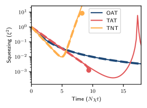
(a) Squeezing with unitary dynamics

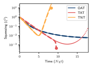
(b) Squeezing with decoherence: $\gamma_{-}=\gamma_{+}=\gamma_{\text{z}}=\chi$

Figure 1: Spin squeezing of $N=10^{4}$ spins initially in $\ket{\text{X}}$ under LABEL:sub@fig:squeezing_unitary unitary and LABEL:sub@fig:squeezing_dec non-unitary dynamics, computed using exact methods (solid lines), quantum trajectory simulations (dots), and the TST expansion in Eq. (10) with $M=35$ (dashed lines). Solid circles mark the times at which the TST expansion gives an unphysical result with $\xi^{2}<0$.

Figure 1 compares the squeezing parameter $\xi^{2}$ for $N=10^{4}$ spins initially in the state $\ket{\text{X}}$ evolved under the Hamiltonians in Eqs. (11)–(13), as computed via both benchmarking simulations and the TST expansion in Eq. (10) with $M=35$. Squeezing is shown for both unitary dynamics (Figure 1a), as well as non-unitary dynamics in the presence of spontaneous decay, excitation, and dephasing of individual spins at rates $\chi$ (Figure 1b), respectively described by the sets of jump operators $\mathcal{J}_{\alpha}\equiv\set{\hat{s}_{\alpha}^{(j)}}$ with corresponding decoherence rates $\gamma_{\alpha}=\chi$ for $\alpha\in\set{-,+,\text{z}}$. The results shown in Figure 1 were computed in a rotated basis with $\left(\hat{s}_{\text{z}},\hat{s}_{\text{x}}\right)\to\left(\hat{s}_{\text{x}},-\hat{s}_{\text{z}}\right)$ and $\ket{\text{X}}\to\ket{-\text{Z}}\equiv\ket{\downarrow}^{\otimes N}$, as well as appropriate transformations of the Hamiltonian and jump operators. The only effects of this rotation on the results presented in Figure 1 are to 1. reduce the time it takes to compute correlators $\braket{\hat{\mathcal{O}}\left(t\right)}$ with the TST expansion, and 2. prolong the time for which the TST expansion of TNT results agree with benchmarking simulations. The speedup in a different basis occurs because for the initial state $\ket{-\text{Z}}$, all initial-time correlators $\braket{\hat{S}_{\bm{m}}}$ are zero unless $m_{+}=m_{-}=0$, and all non-zero correlators take $O\left(1\right)$ (i.e. constant in $N$) time to compute, rather than $O\left(N\right)$ time (see Appendix I). In total, the use of a rotated basis reduces the computation time of initial-time correlators from $O\left(M^{3}N\right)$ to $O\left(M\right)$. The reason for prolonged agreement of TNT results in a rotated basis is not entirely understood, and provides a clue into the precise mechanism by which the TST expansion breaks down (discussed below). We defer a detailed study of this breakdown to future work.

The main lesson from Figure 1 is that the TST expansion yields essentially exact results right up until a sudden and drastic departure that can be diagnosed by inspection. The breakdown of the TST expansion in Figure 1 induces an unphysical squeezing parameter $\xi^{2}<0$. In general, however, there is no fundamental relationship between the breakdown of the TST expansion and the conditions for a physical squeezing parameter $\xi^{2}$. A proper diagnosis of breakdown therefore requires inspection of the correlators $\braket{\hat{\mathcal{S}}_{\bm{n}}\left(t\right)}$ used to compute the squeezing parameter $\xi^{2}$, which upon breakdown will rapidly take unphysical values with $\lvert\braket{\hat{\mathcal{S}}_{\bm{n}}\left(t\right)}\rvert\gtrsim S^{\lvert\bm{n}\rvert}$ (see Appendix L for an example). The sudden and drastic departure from virtually exact results is consistent with the limitations of the TST expansion discussed at the end of Section II. Specifically, we identify three possible mechanisms for breakdown: 1. a rapid growth in the order $M$ necessary for the TST expansion to converge, 2. the growth of numerical errors in excessively large terms of the TST expansion, and 3. the formal breakdown of the perturbative expansion in the time $t$. In all of these cases, a detailed cancellation eventually ceases to occur between large terms at high orders in the TST expansion. These large terms grow with the time $t$ raised to some large power (as high as $M$), and therefore rapidly yield wildly unphysical results. In contrast to other approximate methods such as the cumulant expansionMeiser and Holland (2010), the TST expansion can thus diagnose its own breakdown, which is an important feature when working in parameter regimes that are inaccessible via other means to compute correlators. Note that, due to the breakdown mechanisms of the TST expansion, going up through order $M=70$ does not significantly increase the breakdown time $t_{\text{break}}^{(M)}$ in Figure 1, and in some cases even shortens $t_{\text{break}}^{(M)}$.

Although the TST expansion breaks down at short times, it has two key advantages over the quantum trajectory Monte Carlo method to compute correlators in the presence of decoherence. First, computing spin correlators with the TST expansion is generally faster and requires fewer computing resources. The TST expansion results in Figure 1b, for example, take $\sim 10$ seconds to compute with a single CPU on modern computing hardware. The quantum trajectory Monte Carlo results in the same figure, meanwhile, take $\sim 10^{4}$ CPU hours to compute on similar hardware; the bulk of this time is spent performing sparse matrix-vector multiplication, leaving little room to further optimize serial runtime. Parallelization can reduce actual runtime of the Monte Carlo simulations to $\sim 10$ hours by running all trajectories at once, but at the cost of greatly increasing computing resource requirements. Though it may be possible to further speed up quantum trajectory Monte Carlo simulations by introducing new truncation schemes, any modifications 1. should be made carefully to ensure that simulations still yield correct results, and 2. are unlikely to bridge the orders of magnitude in computing resource requirements.

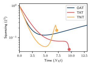
Figure 2: Spin squeezing of $N=10^{4}$ spins initially in $\ket{\text{X}}$ with spontaneous decay, excitation, and dephasing of individual spins at rates $\gamma_{-}=\gamma_{+}=\gamma_{\text{z}}=100\chi$. Computed using the TST expansion in Eq. (10) with $M=35$. Solid circles mark the times at which the TST expansion gives an unphysical result with $\xi^{2}<0$.

The second advantage of the TST expansion is the capability to compute spin correlators in strong-decoherence regimes of large systems that are entirely inaccessible to other methods. As an example, Figure 2 shows squeezing of $N=10^{4}$ spins initially in $\ket{\text{X}}$, undergoing spontaneous decay, excitation, and dephasing of individual spins at rates $\gamma_{-}=\gamma_{+}=\gamma_{\text{z}}=100\chi$. The system size in these simulations is too large for straightforward application of exact methods for open quantum systems. Quantum trajectory Monte Carlo simulations, meanwhile, take a prohibitively long time to converge with such strong decoherence due to the multiplicity of quantum trajectories that require averaging.

The results in Figure 2 show that the TNT model can generate more squeezing than the OAT or TAT models in the presence of strong decoherence. The better performance of TNT is in part a consequence of the fact that TNT initially generates squeezing at a faster rate than OAT or TAT, thereby allowing it to produce more squeezing before the degrading effects of decoherence kick in. We corroborate this finding with quantum trajectory simulations of a smaller system in Appendix M. Strong-decoherence computations of the sort used for Figure 2 put lower bounds on theoretically achievable spin squeezing via TAT with decoherence in Ref. [48], exemplifying a concrete and practical application of the TST expansion and the collective-spin structure constants calculated in this work.

IV Two-time correlation functions and out-of-time-ordered correlators

As a final example of collective-spin physics that is numerically accessible via the TST expansion of Heisenberg operators, we consider the calculation of two-time correlation functions and out-of-time-ordered correlators (OTOCs). In particular, we consider the effect of decoherence on short-time behavior of the two-time connected correlator

$$C\left(t\right)\equiv\dfrac{1}{S}\left(\braket{\hat{S}_{+}\left(t\right)\hat{S}_{-}\left(0\right)}-\braket{\hat{S}_{+}\left(t\right)}\braket{\hat{S}_{-}\left(0\right)}\right),$$ (15)

and the expectation value of a squared commutator,

$$D\left(t\right)\equiv\dfrac{1}{S^{2}}\Braket{\left[\hat{S}_{+}\left(t\right),\hat{S}_{-}\left(0\right)\right]_{-}^{\dagger}\left[\hat{S}_{+}\left(t\right),\hat{S}_{-}\left(0\right)\right]_{-}}_{\text{nn}},$$ (16)

in the context of the squeezing models in Section III. The subscript on $\braket{\cdot}_{\text{nn}}$ in Eq. (16) stands for “no noise”, and denotes a correlator computed without the noise contributions $\hat{\mathcal{E}}_{\mathcal{O}}\left(t\right)$ to Heisenberg operators $\hat{\mathcal{O}}\left(t\right)$. While linear contributions from noise operators as e.g. in Eq. (15) always vanish under Markovian decoherence (see Appendix N), quadratic contributions that would otherwise appear in Eq. (16) generally do notBlocher and Mølmer (2019). Determining the effect of these noise terms generally requires making additional assumptions about the environment, which would be a digression for the purposes of the present work. We therefore exclude these noise terms in (16) in order to keep our discussion simple and general; see Ref. [65] for more detailed discussions of noise terms and the quantum regression theorem underlying the calculation of multi-time correlators.

In an equilibrium setting, correlation functions similar to that in Eq. (15) contain information about the linear response of Heisenberg operators to perturbations of a system; in a non-equilibrium setting, they contribute to short-time linear response (see Appendix O). Similar correlators have made appearances as order parameters for diagnosing time-crystalline phases of matterTucker et al. (2018). Squared commutators such as that in Eq. (16), meanwhile, are commonly examined for signatures of quantum chaos and information scramblingMaldacena et al. (2016); Swingle (2018); García-Mata et al. (2018). In typical scenarios, such squared commutators initially vanish by construction through a choice of spatially separated operators. Collective spin systems, however, have no intrinsic notion of locality or spatial separation. In our case, therefore, with the choice of initial state $\ket{\text{X}}\propto\left(\ket{\uparrow}+\ket{\downarrow}\right)^{\otimes N}$ we merely have $D\left(0\right)\sim 1/N$.

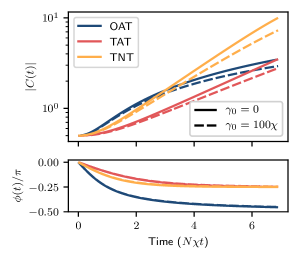
(a) Two-time correlator $C\left(t\right)\equiv\lvert C\left(t\right)\rvert\exp\left[i\phi\left(t\right)\right]$.

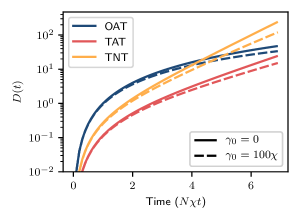
(b) Squared commutator $D\left(t\right)$.

Figure 3: The two-time connected correlator $C\left(t\right)$ and squared commutator $D\left(t\right)$, respectively defined in Eqs. (15) and (16), for $N=10^{4}$ spins initially in the polarized state $\ket{\text{X}}\propto\left(\ket{\uparrow}+\ket{\downarrow}\right)^{\otimes N}$ evolving under the squeezing Hamiltonians in Eqs. (11)–(13). Results are shown for both unitary dynamics (solid lines) and non-unitary dynamics with $\gamma_{-}=\gamma_{+}=\gamma_{\text{z}}=\gamma_{0}=100\chi$ (dashed lines), computed using the TST expansion in Eq. (10) with $M=20$.

Figure 3 shows the behavior of $C\left(t\right)$ and $D\left(t\right)$ for $N=10^{4}$ spins, initially in the state $\ket{\text{X}}$, evolving under the squeezing Hamiltonians in Eqs. (11)–(13) both with and without spontaneous decay, excitation, and dephasing of individual spins at rates $\gamma_{-}=\gamma_{+}=\gamma_{\text{z}}=100\chi$. In the case of unitary evolution under OAT, we find that to an excellent approximation $\lvert C\left(t\right)\rvert$ takes the functional form $f\left(t\right)=f\left(0\right)+aN\chi t+\left(bN\chi t\right)^{2}$ with $a\sim b\sim 1$, and with a virtually perfect fit $D\left(t\right)=D\left(0\right)+\left(\left[N+1\right]\chi t\right)^{2}$. For unitary evolution under TAT and TNT, we find that to an excellent approximation both $\lvert C\left(t\right)\rvert$ and $D\left(t\right)$ take the functional form $f\left(t\right)=f\left(0\right)+a\left[\exp\left(bN\chi t\right)-1\right]$ with $a\sim b\sim 1$. As may be expected, the growth of $C\left(t\right)$ and $D\left(t\right)$ is generally suppressed by decoherence. Figure 3 serves as an example for the type of behavior that is accessible at short times with the TST expansion. These examples are straightforward to extend to equilibrium settings and spin-boson systems.

V Conclusions

We have presented an efficient method for computing correlators at short times in collective spin systems. This method is based on truncating a short-time expansion of Heisenberg operators, and can access correlators on time scales that are relevant to metrological applications such as spin squeezing. In order to evaluate the truncated short-time (TST) expansion of Heisenberg operators, we have computed the structure constants of a collective spin operator algebra, which we hope will empower future analytical and numerical studies of collective spin systems. Even though we considered only non-equilibrium spin-squeezing processes in this work, our method can be applied directly in an equilibrium setting, and is straightforward to generalize to systems such as trapped ions and optical cavities with collective spin-boson interactions. In such contexts, our method may be used to benchmark the short-time effects of decoherence, or study the onset of quantum chaos and information scrambling.

Appendix A Basic spin operator identities

The appendices in this work make ubiquitous use of various spin operator identities; we collect and derive some basic identities here for reference. Note that despite the working definition of collective spin operators from $S_{\alpha}=\sum_{j}s_{\alpha}^{(j)}$, the identities we will derive involving only collective spin operators apply just as well to large-spin operators that cannot be expressed as the sum of individual spin-1/2 operators. The elementary commutation relations between spin operators are, with ${\bar{\mu}}\equiv-\mu\in\set{+1,-1}$ for brevity,

$$\left[s_{\text{z}}^{(j)},s_{\mu}^{(k)}\right]_{-} =\delta_{jk}\mu s_{\mu}^{(j)}, \left[S_{\text{z}},s_{\mu}^{(j)}\right]_{-} =\left[s_{\text{z}}^{(j)},S_{\mu}\right]_{-}=\mu s_{\mu}^{(j)}, \left[S_{\text{z}},S_{\mu}\right]_{-} =\mu S_{\mu},$$ (17)

$$\left[s_{\mu}^{(j)},s_{\bar{\mu}}^{(k)}\right]_{-} =\delta_{jk}2\mu s_{\text{z}}^{(j)}, \left[S_{\mu},s_{\bar{\mu}}^{(j)}\right]_{-} =\left[s_{\mu}^{(j)},S_{\bar{\mu}}\right]_{-}=2\mu s_{\text{z}}^{(j)}, \left[S_{\mu},S_{\bar{\mu}}\right]_{-} =2\mu S_{\text{z}}.$$ (18)

These relations can be used to inductively compute identities involving powers of collective spin operators. By pushing through one spin operator at a time, we can find

$$\left(\mu S_{\text{z}}\right)^{m}s_{\mu}^{(j)}=\left(\mu S_{\text{z}}\right)^{m-1}s_{\mu}^{(j)}\left(1+\mu S_{\text{z}}\right)=\left(\mu S_{\text{z}}\right)^{m-2}s_{\mu}^{(j)}\left(1+\mu S_{\text{z}}\right)^{2}=\cdots=s_{\mu}^{(j)}\left(1+\mu S_{\text{z}}\right)^{m},$$ (19)

and

$$\mu s_{\text{z}}^{(j)}S_{\mu}^{m}=S_{\mu}\mu s_{\text{z}}^{(j)}S_{\mu}^{m-1}+s_{\mu}^{(j)}S_{\mu}^{m-1}=\cdots=S_{\mu}^{m}\mu s_{\text{z}}^{(j)}+ms_{\mu}^{(j)}S_{\mu}^{m-1},$$ (20)

where we will generally find it nicer to express results in terms of $\mu s_{\text{z}}^{(j)}$ and $\mu S_{\text{z}}$ rather than $s_{\text{z}}^{(j)}$ and $S_{\text{z}}$. Summing over the single-spin index $j$ in both of the cases above gives us the purely collective-spin versions of these identities:

$$\left(\mu S_{\text{z}}\right)^{m}S_{\mu}=S_{\mu}\left(1+\mu S_{\text{z}}\right)^{m}, \mu S_{\text{z}}S_{\mu}^{m}=S_{\mu}^{m}\left(m+\mu S_{\text{z}}\right),$$ (21)

where we can repeat the process of pushing through individual $S_{\text{z}}$ operators $\ell$ times to get

$$\left(\mu S_{\text{z}}\right)^{\ell}S_{\mu}^{m}=\left(\mu S_{\text{z}}\right)^{\ell-1}S_{\mu}^{m}\left(m+\mu S_{\text{z}}\right)=\left(\mu S_{\text{z}}\right)^{\ell-2}S_{\mu}^{m}\left(m+\mu S_{\text{z}}\right)^{2}=\cdots=S_{\mu}^{m}\left(m+\mu S_{\text{z}}\right)^{\ell}.$$ (22)

Multiplying (22) through by $\left(\mu\nu\right)^{\ell}$ (for $\nu\in\set{+1,-1}$) and taking its Hermitian conjugate, we can say that more generally

$$\left(\nu S_{\text{z}}\right)^{\ell}S_{\mu}^{m}=S_{\mu}^{m}\left(\mu\nu m+\nu S_{\text{z}}\right)^{\ell}, S_{\mu}^{m}\left(\nu S_{\text{z}}\right)^{\ell}=\left(-\mu\nu m+\nu S_{\text{z}}\right)^{\ell}S_{\mu}^{m}.$$ (23)

Finding commutation relations between powers of transverse spin operators, i.e. $S_{\mu}$ and $S_{\bar{\mu}}$, turns out to be considerably more difficult than the cases we have worked out thus far. We therefore save this work for Appendix B.

Appendix B Commutation relations between powers of transverse spin operators

To find commutation relations between powers of transverse collective spin operators, we first compute

$$S_{\mu}^{m}s_{\bar{\mu}}^{(j)} =S_{\mu}^{m-1}s_{\bar{\mu}}^{(j)}S_{\mu}+S_{\mu}^{m-1}2\mu s_{\text{z}}^{(j)}$$ (24)

$$=S_{\mu}^{m-2}s_{\bar{\mu}}^{(j)}S_{\mu}^{2}+S_{\mu}^{m-2}2\mu s_{\text{z}}^{(j)}S_{\mu}+S_{\mu}^{m-1}2\mu s_{\text{z}}^{(j)}$$ (25)

$$=s_{\bar{\mu}}^{(j)}S_{\mu}^{m}+\sum_{k=0}^{m-1}S_{\mu}^{k}2\mu s_{\text{z}}^{(j)}S_{\mu}^{m-k-1}.$$ (26)

While (26) gives us the commutator $\left[S_{\mu}^{m},s_{\bar{\mu}}^{(j)}\right]_{-}$, we would like to enforce an ordering on products of spin operators, which will ensure that we only keep track of operators that are linearly independent. We choose (for now) to impose an ordering with all $s_{\bar{\mu}}^{(j)}$ operators on the left, and all $s_{\text{z}}^{(j)}$ operators on the right. Such an ordering will prove convenient for the calculations in this section. This choice of ordering compels us to expand

$$\sum_{k=0}^{m-1}S_{\mu}^{k}2\mu s_{\text{z}}^{(j)}S_{\mu}^{m-k-1} =\sum_{k=0}^{m-1}S_{\mu}^{k}\left[2\left(m-k-1\right)s_{\mu}^{(j)}S_{\mu}^{m-k-2}+S_{\mu}^{m-k-1}2\mu s_{\text{z}}^{(j)}\right]$$ (27)

$$=m\left(m-1\right)s_{\mu}^{(j)}S_{\mu}^{m-2}+mS_{\mu}^{m-1}2\mu s_{\text{z}}^{(j)},$$ (28)

which implies

$$S_{\mu}^{m}s_{\bar{\mu}}^{(j)}=s_{\bar{\mu}}^{(j)}S_{\mu}^{m}+m\left(m-1\right)s_{\mu}^{(j)}S_{\mu}^{m-2}+mS_{\mu}^{m-1}2\mu s_{\text{z}}^{(j)},$$ (29)

and in turn

$$S_{\mu}^{m}S_{\bar{\mu}}=S_{\bar{\mu}}S_{\mu}^{m}+mS_{\mu}^{m-1}\left(m-1+2\mu S_{\text{z}}\right).$$ (30)

As the next logical step, we take on the task of computing

$$S_{\mu}^{m}S_{\bar{\mu}}^{n}=S_{\mu}^{m-1}S_{\bar{\mu}}^{n}S_{\mu}+n\left[S_{\mu}^{m-1}S_{\bar{\mu}}^{n-1}\left(1-n+2\mu S_{\text{z}}\right)\right]=S_{\bar{\mu}}^{n}S_{\mu}^{m}+n\sum_{k=0}^{m-1}S_{\mu}^{m-k-1}S_{\bar{\mu}}^{n-1}\left(1-n+2\mu S_{\text{z}}\right)S_{\mu}^{k},$$ (31)

which implies

$$\left[S_{\mu}^{m},S_{\bar{\mu}}^{n}\right]_{-}=C_{mn;\mu}\equiv n\sum_{k=0}^{m-1}S_{\mu}^{m-k-1}S_{\bar{\mu}}^{n-1}\left(1-n+2\mu S_{\text{z}}\right)S_{\mu}^{k}.$$ (32)

We now need to rearrange the operators in $C_{mn;\mu}$ into a standard order, which means pushing all $S_{\text{z}}$ operators to the right and, for the purposes of this calculation, all $S_{\bar{\mu}}$ operators to the left. We begin by pushing $S_{\mu}^{k}$ to the left of $S_{\text{z}}$, which takes $2\mu S_{\text{z}}\to 2\mu S_{\text{z}}+2k$, and then push $S_{\mu}^{m-k-1}$ to the right of $S_{\bar{\mu}}^{n-1}$, giving us

$$C_{mn;\mu} =n\sum_{k=0}^{m-1}\left(S_{\bar{\mu}}^{n-1}S_{\mu}^{m-k-1}+C_{m-k-1,n-1;\mu}\right)S_{\mu}^{k}\left(2k+1-n+2\mu S_{\text{z}}\right)$$ (33)

$$=D_{mn;\mu}+n\sum_{k=0}^{m-2}C_{m-k-1,n-1;\mu}S_{\mu}^{k}\left(2k+1-n+2\mu S_{\text{z}}\right),$$ (34)

where we have dropped the last ($k=m-1$) term in the remaining sum because $C_{m-k-1,n-1;\mu}=0$ if $k=m-1$, and

$$D_{mn;\mu}\equiv mnS_{\bar{\mu}}^{n-1}S_{\mu}^{m-1}\left(m-n+2\mu S_{\text{z}}\right).$$ (35)

To our despair, we have arrived in (34) at a recursive formula for $C_{mn;\mu}$. Furthermore, we have not even managed to order all spin operators, as $C_{m-k-1,n-1;\mu}$ contains $S_{\text{z}}$ operators that are to the left of $S_{\mu}^{k}$. To sort all spin operators once and for all, we define

$$C_{mn;\mu}^{(k)}\equiv C_{m-k,n;\mu}S_{\mu}^{k}, D_{mn;\mu}^{(k)}\equiv D_{m-k,n;\mu}S_{\mu}^{k},$$ (36)

which we can expand as

$$D_{mn;\mu}^{(k)} =\left(m-k\right)nS_{\bar{\mu}}^{n-1}S_{\mu}^{m-k-1}\left(m-k-n+2\mu S_{\text{z}}\right)S_{\mu}^{k}$$ (37)

$$=\left(m-k\right)nS_{\bar{\mu}}^{n-1}S_{\mu}^{m-1}\left(k+m-n+2\mu S_{\text{z}}\right),$$ (38)

and

$$C_{mn;\mu}^{(k)} =D_{m-k,n;\mu}S_{\mu}^{k}+n\sum_{j=0}^{m-k-2}C_{m-k-j-1,n-1;\mu}S_{\mu}^{j}\left(2j+1-n+2\mu S_{\text{z}}\right)S_{\mu}^{k}$$ (39)

$$=D_{mn;\mu}^{(k)}+n\sum_{j=0}^{m-k-2}C_{m-k-j-1,n-1;\mu}S_{\mu}^{j+k}\left(2j+2k+1-n+2\mu S_{\text{z}}\right)$$ (40)

$$=D_{mn;\mu}^{(k)}+n\sum_{j=0}^{m-k-2}C_{m-1,n-1;\mu}^{(k+j)}\left(2\left[j+k\right]+1-n+2\mu S_{\text{z}}\right)$$ (41)

$$=D_{mn;\mu}^{(k)}+n\sum_{j=k}^{m-2}C_{m-1,n-1;\mu}^{(j)}\left(2j+1-n+2\mu S_{\text{z}}\right).$$ (42)

While the resulting expression in (42) strongly resembles that in (34), there is one crucial difference: all spin operators in (42) have been sorted into a standard order. We can now repeatedly substitute $C_{mn;\mu}^{(k)}$ into itself, each time decreasing $m$ and $n$ by 1, until one of $m$ or $n$ reaches zero. Such repeated substitution yields the expansion

$$C_{mn;\mu}=C_{mn;\mu}^{(0)}=D_{mn;\mu}+\sum_{p=1}^{\min\set{m,n}-1}E_{mn;\mu}^{(p)},$$ (43)

where the first two terms in the sum over $p$ are

$$E_{mn;\mu}^{(1)} =n\sum_{k=0}^{m-2}D_{m-1,n-1;\mu}^{(k)}\left(2k+1-n+2\mu S_{\text{z}}\right),$$ (44)

$$E_{mn;\mu}^{(2)} =n\sum_{k_{1}=0}^{m-2}\left(n-1\right)\sum_{k_{2}=k_{1}}^{m-3}D_{m-2,n-2;\mu}^{(k_{2})}\left(2k_{2}+2-n+2\mu S_{\text{z}}\right)\left(2k_{1}+1-n+2\mu S_{\text{z}}\right),$$ (45)

and more generally for $p>1$,

$$E_{mn;\mu}^{(p)}=\dfrac{n!}{\left(n-p\right)!}\sum_{k_{1}=0}^{m-2}\sum_{k_{2}=k_{1}}^{m-3}\cdots\sum_{k_{p}=k_{p-1}}^{m-p-1}D_{m-p,n-p;\mu}^{(k_{p})}\prod_{j=1}^{p}\left(2k_{j}+j-n+2\mu S_{\text{z}}\right).$$ (46)

In principle, the expressions in (35), (38), (43), and (46) suffice to evaluate the commutator $\left[S_{\mu}^{m},S_{\bar{\mu}}^{n}\right]_{-}=C_{mn;\mu}$, but this result is – put lightly – quite a mess: the expression for $E_{mn;\mu}^{(p)}$ in (46) involves a sum over $p$ mutually dependent intermediate variables, each term of which additionally contains a product of $p$ factors. We therefore devote the rest of this section to simplifying our result for the commutator $\left[S_{\mu}^{m},S_{\bar{\mu}}^{n}\right]_{-}$.

Observing that in (46) we always have $0\leq k_{1}\leq k_{2}\leq\cdots\leq k_{p}\leq m-p-1$, we can rearrange the order of the sums and relabel $k_{p}\to\ell$ to get

$$E_{mn;\mu}^{(p)}=\dfrac{n!}{\left(n-p\right)!}\sum_{\ell=0}^{m-p-1}D_{m-p,n-p;\mu}^{(\ell)}\left(2\ell+F_{np;\mu}\right)\sum_{\left(\bm{k},p-1,\ell\right)}\prod_{j=1}^{p-1}\left(2k_{p-j}-j+F_{np;\mu}\right),$$ (47)

where for shorthand we define

$$F_{np;\mu}\equiv p-n+2\mu S_{\text{z}}, \sum_{\left(\bm{k},q,\ell\right)}X\equiv\sum_{k_{1}=0}^{\ell}\sum_{k_{2}=k_{1}}^{\ell}\cdots\sum_{k_{q}=k_{q-1}}^{\ell}X.$$ (48)

We now further define

$$f_{np\ell;\mu}\left(k,q\right)\equiv\left(\ell-k+q\right)\left(\ell+k-q+F_{np;\mu}\right),$$ (49)

and evaluate sums successively over $k_{p-1},k_{p-2},\cdots,k_{1}$, finding

$$\sum_{\left(\bm{k},p-1,\ell\right)}\prod_{j=1}^{p-1}\left(2k_{p-j}-j+F_{np;\mu}\right) =\sum_{\left(\bm{k},p-2,\ell\right)}\prod_{j=2}^{p-1}\left(2k_{p-j}-j+F_{np;\mu}\right)f_{np\ell;\mu}\left(k_{p-2},1\right)$$ (50)

$$=\dfrac{1}{\left(r-1\right)!}\sum_{\left(\bm{k},p-r,\ell\right)}\prod_{j=r}^{p-1}\left(2k_{p-j}-j+F_{np;\mu}\right)\prod_{q=1}^{r-1}f_{np\ell;\mu}\left(k_{p-r},q\right)$$ (51)

$$=\dfrac{1}{\left(p-1\right)!}\prod_{q=1}^{p-1}f_{np\ell;\mu}\left(0,q\right)$$ (52)

$$={\ell+p-1\choose p-1}\prod_{q=1}^{p-1}\left(\ell-q+F_{np;\mu}\right).$$ (53)

Substitution of this result together with $D_{m-p,n-p;\mu}^{(\ell)}$ using (38) into (47) then gives us

$$E_{mn;\mu}^{(p)}=\dfrac{n!}{\left(n-p-1\right)!}S_{\bar{\mu}}^{n-p-1}S_{\mu}^{m-p-1}G_{mnp;\mu}$$ (54)

with

$$G_{mnp;\mu} \equiv\sum_{\ell=0}^{m-p-1}{\ell+p-1\choose p-1}\left(m-p-\ell\right)\left(\ell+m-p+F_{np;\mu}\right)\left(2\ell+F_{np;\mu}\right)\prod_{q=1}^{p-1}\left(\ell-q+F_{np;\mu}\right)$$ (55)

$$={m\choose p+1}\prod_{q=0}^{p}\left(m-p-q+F_{np;\mu}\right).$$ (56)

We can further simplify

$$\prod_{q=0}^{p}\left(m-p-q+F_{np;\mu}\right)=\prod_{q=0}^{p}\left(m-n-q+2\mu S_{\text{z}}\right)=\sum_{q=0}^{p+1}\left(-1\right)^{p+1-q}{p+1\brack q}\left(m-n+2\mu S_{\text{z}}\right)^{q},$$ (57)

where ${p\brack q}$ is an unsigned Stirling number of the first kind, and finally

$$\sum_{q=0}^{p}\left(-1\right)^{p-q}{p\brack q}\left(m-n+2\mu S_{\text{z}}\right)^{q} =\sum_{q=0}^{p}\left(-1\right)^{p-q}{p\brack q}\sum_{\ell=0}^{q}{q\choose\ell}\left(m-n\right)^{q-\ell}\left(2\mu S_{\text{z}}\right)^{\ell}$$ (58)

$$=\sum_{\ell=0}^{p}2^{\ell}\sum_{q=\ell}^{p}\left(-1\right)^{p-q}{p\brack q}{q\choose\ell}\left(m-n\right)^{q-\ell}\left(\mu S_{\text{z}}\right)^{\ell}.$$ (59)

Putting everything together, we finally have

$$E_{mn;\mu}^{(p-1)}=p!{m\choose p}{n\choose p}S_{\bar{\mu}}^{n-p}S_{\mu}^{m-p}\sum_{\ell=0}^{p}\epsilon_{mn}^{p\ell}\left(\mu S_{\text{z}}\right)^{\ell},$$ (60)

with

$$\epsilon_{mn}^{p\ell}\equiv 2^{\ell}\sum_{q=\ell}^{p}\left(-1\right)^{p-q}{p\brack q}{q\choose\ell}\left(m-n\right)^{q-\ell},$$ (61)

where in this final form $E_{mn;\mu}^{(0)}=D_{mn;\mu}$, which together with the expansion for $C_{mn;\mu}$ in (43) implies that

$$\left[S_{\mu}^{m},S_{\bar{\mu}}^{n}\right]_{-}=\sum_{p=1}^{\min\set{m,n}}p!{m\choose p}{n\choose p}S_{\bar{\mu}}^{n-p}S_{\mu}^{m-p}\sum_{\ell=0}^{p}\epsilon_{mn}^{p\ell}\left(\mu S_{\text{z}}\right)^{\ell},$$ (62)

and

$$S_{\mu}^{m}S_{\bar{\mu}}^{n}=\sum_{p=0}^{\min\set{m,n}}p!{m\choose p}{n\choose p}S_{\bar{\mu}}^{n-p}S_{\mu}^{m-p}\sum_{\ell=0}^{p}\epsilon_{mn}^{p\ell}\left(\mu S_{\text{z}}\right)^{\ell}.$$ (63)

If we wish to order products of collective spin operators with $S_{\text{z}}$ in between $S_{\bar{\mu}}$ and $S_{\mu}$, then

$$S_{\mu}^{m}S_{\bar{\mu}}^{n}=\sum_{p=0}^{\min\set{m,n}}p!{m\choose p}{n\choose p}S_{\bar{\mu}}^{n-p}Z_{mn;{\bar{\mu}}}^{(p)}S_{\mu}^{m-p},$$ (64)

where

$$Z_{mn;{\bar{\mu}}}^{(p)}\equiv\sum_{\ell=0}^{p}\epsilon_{mn}^{p\ell}\left(-\left[m-p\right]+\mu S_{\text{z}}\right)^{\ell}=\sum_{q=0}^{p}\zeta_{mn}^{pq}\left({\bar{\mu}}S_{\text{z}}\right)^{q},$$ (65)

with

$$\zeta_{mn}^{pq}\equiv\sum_{\ell=q}^{p}\epsilon_{mn}^{p\ell}{\ell\choose q}\left(-1\right)^{\ell}\left(m-p\right)^{\ell-q}=\left(-1\right)^{p}2^{q}\sum_{s=q}^{p}{p\brack s}{s\choose q}\left(m+n-2p\right)^{s-q}.$$ (66)

Here ${p\brack s}$ is an unsigned Stirling number of the first kind.

Appendix C Product of arbitrary ordered collective spin operators

The most general product of collective spin operators that we need to compute is

$$\mathcal{S}^{pqr}_{\ell mn;\mu}=S_{\mu}^{p}\left(\mu S_{\text{z}}\right)^{q}S_{\bar{\mu}}^{r}S_{\mu}^{\ell}\left(\mu S_{\text{z}}\right)^{m}S_{\bar{\mu}}^{n}=\sum_{k=0}^{\min\set{r,\ell}}k!{r\choose k}{\ell\choose k}S_{\mu}^{p+\ell-k}\tilde{Z}_{qr\ell m;\mu}^{(k)}S_{\bar{\mu}}^{r+n-k},$$ (67)

where

$$\tilde{Z}_{qr\ell m;\mu}^{(k)} \equiv\left(\ell-k+\mu S_{\text{z}}\right)^{q}Z_{r\ell;\mu}^{(k)}\left(r-k+\mu S_{\text{z}}\right)^{m}$$ (68)

$$=\sum_{a=0}^{k}\zeta_{r\ell}^{ka}\sum_{b=0}^{q}\left(\ell-k\right)^{q-b}{q\choose b}\sum_{c=0}^{m}\left(r-k\right)^{m-c}{m\choose c}\left(\mu S_{\text{z}}\right)^{a+b+c},$$ (69)

is defined in terms of $Z_{r\ell;\mu}^{(k)}$ and $\zeta_{r\ell}^{ka}$ as respectively given in (65) and (66). The (anti-)commutator of two ordered products of collective spin operators is then simply

$$\left[S_{\mu}^{p}\left(\mu S_{\text{z}}\right)^{q}S_{\bar{\mu}}^{r},S_{\mu}^{\ell}\left(\mu S_{\text{z}}\right)^{m}S_{\bar{\mu}}^{n}\right]_{\pm}=\mathcal{S}^{pqr}_{\ell mn;\mu}\pm\mathcal{S}^{\ell mn}_{pqr;\mu}.$$ (70)

Appendix D Sandwich identities for single-spin decoherence calculations

In this section we derive several identities that will be necessary for computing the effects of single-spin decoherence on ordered products of collective spin operators, i.e. on operators of the form $S_{\mu}^{\ell}\left(\mu S_{\text{z}}\right)^{m}S_{\bar{\mu}}^{n}$. These identities all involve sandwiching a collective spin operator between operators that act on individual spins only, and summing over all individual spin indices. Our general strategy will be to use commutation relations to push single-spin operators together, and then evaluate the sum to arrive at an expression involving only collective spin operators.

We first compute sums of single-spin operators sandwiching $\left(\mu S_{\text{z}}\right)^{m}$, when necessary making use of the identity in (19). The unique cases up to Hermitian conjugation are, for $S\equiv N/2$ and $\mu,\nu\in\set{+1,-1}$,

$$\sum_{j}s_{\text{z}}^{(j)}\left(\mu S_{\text{z}}\right)^{m}s_{\text{z}}^{(j)} =\sum_{j}s_{\text{z}}^{(j)}s_{\text{z}}^{(j)}\left(\mu S_{\text{z}}\right)^{m}=\dfrac{1}{4}\sum_{j}\mathds{1}_{j}\left(\mu S_{\text{z}}\right)^{m}=\dfrac{1}{2}S\left(\mu S_{\text{z}}\right)^{m},$$ (71)

$$\sum_{j}s_{\text{z}}^{(j)}\left(\mu S_{\text{z}}\right)^{m}s_{\nu}^{(j)} =\left(\mu S_{\text{z}}\right)^{m}\sum_{j}s_{\text{z}}^{(j)}s_{\nu}^{(j)}=\dfrac{1}{2}\left(\mu S_{\text{z}}\right)^{m}\nu S_{\nu}=\dfrac{1}{2}\nu S_{\nu}\left(\mu\nu+\mu S_{\text{z}}\right)^{m},$$ (72)

$$\sum_{j}s_{\nu}^{(j)}\left(\mu S_{\text{z}}\right)^{m}s_{\nu}^{(j)} =\sum_{j}s_{\nu}^{(j)}s_{\nu}^{(j)}\left(\mu\nu+\mu S_{\text{z}}\right)^{m}=0,$$ (73)

$$\sum_{j}s_{\bar{\nu}}^{(j)}\left(\mu S_{\text{z}}\right)^{m}s_{\nu}^{(j)} =\sum_{j}s_{\bar{\nu}}^{(j)}s_{\nu}^{(j)}\left(\mu\nu+\mu S_{\text{z}}\right)^{m}=\left(S-\nu S_{\text{z}}\right)\left(\mu\nu+\mu S_{\text{z}}\right)^{m}.$$ (74)

We are now equipped to derive similar identities for more general collective spin operators. Making heavy use of identities (20) and (29) to push single-spin operators through transverse collective-spin operators, we again work through all combinations that are unique up to Hermitian conjugation, finding

$$\sum_{j}s_{\text{z}}^{(j)}S_{\mu}^{\ell}\left(\mu S_{\text{z}}\right)^{m}S_{\bar{\mu}}^{n}s_{\text{z}}^{(j)} =\dfrac{1}{2}\left(S-\ell-n\right)S_{\mu}^{\ell}\left(\mu S_{\text{z}}\right)^{m}S_{\bar{\mu}}^{n}+\ell nS_{\mu}^{\ell-1}\left(S+\mu S_{\text{z}}\right)\left(-1+\mu S_{\text{z}}\right)^{m}S_{\bar{\mu}}^{n-1},\allowdisplaybreaks$$ (75)

$$\sum_{j}s_{\text{z}}^{(j)}S_{\mu}^{\ell}\left(\mu S_{\text{z}}\right)^{m}S_{\bar{\mu}}^{n}s_{\mu}^{(j)} =\dfrac{1}{2}\mu S_{\mu}^{\ell+1}\left(1+\mu S_{\text{z}}\right)^{m}S_{\bar{\mu}}^{n}-\mu n\left(S-\ell-\dfrac{1}{2}\left[n-1\right]\right)S_{\mu}^{\ell}\left(\mu S_{\text{z}}\right)^{m}S_{\bar{\mu}}^{n-1}$$

$$\qquad-\mu\ell n\left(n-1\right)S_{\mu}^{\ell-1}\left(S+\mu S_{\text{z}}\right)\left(-1+\mu S_{\text{z}}\right)^{m}S_{\bar{\mu}}^{n-2},\allowdisplaybreaks$$ (76)

$$\sum_{j}s_{\text{z}}^{(j)}S_{\mu}^{\ell}\left(\mu S_{\text{z}}\right)^{m}S_{\bar{\mu}}^{n}s_{\bar{\mu}}^{(j)} =-\dfrac{1}{2}\mu S_{\mu}^{\ell}\left(\mu S_{\text{z}}\right)^{m}S_{\bar{\mu}}^{n+1}+\mu\ell S_{\mu}^{\ell-1}\left(S+\mu S_{\text{z}}\right)\left(-1+\mu S_{\text{z}}\right)^{m}S_{\bar{\mu}}^{n},\allowdisplaybreaks$$ (77)

$$\sum_{j}s_{\mu}^{(j)}S_{\mu}^{\ell}\left(\mu S_{\text{z}}\right)^{m}S_{\bar{\mu}}^{n}s_{\mu}^{(j)} =nS_{\mu}^{\ell+1}\left(\mu S_{\text{z}}\right)^{m}S_{\bar{\mu}}^{n-1}-n\left(n-1\right)S_{\mu}^{\ell}\left(S+\mu S_{\text{z}}\right)\left(-1+\mu S_{\text{z}}\right)^{m}S_{\bar{\mu}}^{n-2},\allowdisplaybreaks$$ (78)

$$\sum_{j}s_{\mu}^{(j)}S_{\mu}^{\ell}\left(\mu S_{\text{z}}\right)^{m}S_{\bar{\mu}}^{n}s_{\bar{\mu}}^{(j)} =S_{\mu}^{\ell}\left(S+\mu S_{\text{z}}\right)\left(-1+\mu S_{\text{z}}\right)^{m}S_{\bar{\mu}}^{n},\allowdisplaybreaks$$ (79)

$$\sum_{j}s_{\bar{\mu}}^{(j)}S_{\mu}^{\ell}\left(\mu S_{\text{z}}\right)^{m}S_{\bar{\mu}}^{n}s_{\mu}^{(j)} =S_{\mu}^{\ell}\left(S-\ell-n-\mu S_{\text{z}}\right)\left(1+\mu S_{\text{z}}\right)^{m}S_{\bar{\mu}}^{n}+\ell n\left(2S-\ell-n+2\right)S_{\mu}^{\ell-1}\left(\mu S_{\text{z}}\right)^{m}S_{\bar{\mu}}^{n-1}$$

$$\qquad+\ell n\left(\ell-1\right)\left(n-1\right)S_{\mu}^{\ell-2}\left(S+\mu S_{\text{z}}\right)\left(-1+\mu S_{\text{z}}\right)^{m}S_{\bar{\mu}}^{n-2}.$$ (80)

Appendix E Uncorrelated, permutationally-symmetric single-spin decoherence

In this section we work out the effects of permutationally-symmetric decoherence of individual spins on collective spin operators of the form $S_{\mu}^{\ell}\left(\mu S_{\text{z}}\right)^{m}S_{\bar{\mu}}^{n}$. For compactness, we define

$$\mathcal{D}\left(g\right)\mathcal{O}\equiv\mathcal{D}\left(\set{g^{(j)}\mathrel{\mathop{\mathchar 58\relax}}j=1,2,\cdots,N}\right)\mathcal{O}=\sum_{j}\left({g^{(j)}}^{\dagger}\mathcal{O}g^{(j)}-\dfrac{1}{2}\left[{g^{(j)}}^{\dagger}g^{(j)},\mathcal{O}\right]_{+}\right),$$ (81)

where $g$ is an operator that acts on a single spin, $g^{(j)}$ is an operator that acts with $g$ on spin $j$ and trivially on all other spins, and $N$ is the total number of spins.

E.1 Decay-type decoherence

The effect of decoherence via uncorrelated decay ($\mu=-1$) or excitation ($\mu=1$) of individual spins is described by

$$\mathcal{D}\left(s_{\mu}\right)\mathcal{O}=\sum_{j}\left(s_{\bar{\mu}}^{(j)}\mathcal{O}s_{\mu}^{(j)}-\dfrac{1}{2}\left[s_{\bar{\mu}}^{(j)}s_{\mu}^{(j)},\mathcal{O}\right]_{+}\right)=\sum_{j}s_{\bar{\mu}}^{(j)}\mathcal{O}s_{\mu}^{(j)}-S\mathcal{O}+\dfrac{\mu}{2}\left[S_{\text{z}},\mathcal{O}\right]_{+}.$$ (82)

In order to determine the effect of this decoherence on general collective spin operators, we expand the anti-commutator

$$\left[S_{\text{z}},S_{\mu}^{\ell}\left(\mu S_{\text{z}}\right)^{m}S_{\bar{\mu}}^{n}\right]_{+}=S_{\text{z}}S_{\mu}^{\ell}\left(\mu S_{\text{z}}\right)^{m}S_{\bar{\mu}}^{n}+S_{\mu}^{\ell}\left(\mu S_{\text{z}}\right)^{m}S_{\bar{\mu}}^{n}S_{\text{z}}=\mu S_{\mu}^{\ell}\left(\ell+n+2\mu S_{\text{z}}\right)\left(\mu S_{\text{z}}\right)^{m}S_{\bar{\mu}}^{n},$$ (83)

which implies, using (79),

$$\mathcal{D}\left(s_{\bar{\mu}}\right)\left(S_{\mu}^{\ell}\left(\mu S_{\text{z}}\right)^{m}S_{\bar{\mu}}^{n}\right)=S_{\mu}^{\ell}\left(S+\mu S_{\text{z}}\right)\left(-1+\mu S_{\text{z}}\right)^{m}S_{\bar{\mu}}^{n}-S_{\mu}^{\ell}\left[S+\dfrac{1}{2}\left(\ell+n\right)+\mu S_{\text{z}}\right]\left(\mu S_{\text{z}}\right)^{m}S_{\bar{\mu}}^{n},$$ (84)

and, using (80),

$$\mathcal{D}\left(s_{\mu}\right)\left(S_{\mu}^{\ell}\left(\mu S_{\text{z}}\right)^{m}S_{\bar{\mu}}^{n}\right) =S_{\mu}^{\ell}\left(S-\ell-n-\mu S_{\text{z}}\right)\left(1+\mu S_{\text{z}}\right)^{m}S_{\bar{\mu}}^{n}-S_{\mu}^{\ell}\left[S-\dfrac{1}{2}\left(\ell+n\right)-\mu S_{\text{z}}\right]\left(\mu S_{\text{z}}\right)^{m}S_{\bar{\mu}}^{n}$$

$$\qquad+\ell n\left(2S-\ell-n+2\right)S_{\mu}^{\ell-1}\left(\mu S_{\text{z}}\right)^{m}S_{\bar{\mu}}^{n-1}$$

$$\qquad+\ell n\left(\ell-1\right)\left(n-1\right)S_{\mu}^{\ell-2}\left(S+\mu S_{\text{z}}\right)\left(-1+\mu S_{\text{z}}\right)^{m}S_{\bar{\mu}}^{n-2}.$$ (85)

Decoherence via jump operators $s_{\bar{\mu}}^{(j)}$ only couples operators $S_{\mu}^{\ell}\left(\mu S_{\text{z}}\right)^{m}S_{\bar{\mu}}^{n}$ to operators $S_{\mu}^{\ell}\left(\mu S_{\text{z}}\right)^{m^{\prime}}S_{\bar{\mu}}^{n}$ with $m^{\prime}\leq m$. Decoherence via jump operators $s_{\mu}^{(j)}$, meanwhile, makes operators $S_{\mu}^{\ell}\left(\mu S_{\text{z}}\right)^{m}S_{\bar{\mu}}^{n}$ “grow” in $m$ through the last term in (85), although the sum $\ell+m+n$ does not grow.

E.2 Dephasing

The effect of decoherence via single-spin dephasing is described by

$$\mathcal{D}\left(s_{\text{z}}\right)\mathcal{O}=\sum_{j}\left(s_{\text{z}}^{(j)}\mathcal{O}s_{\text{z}}^{(j)}-\dfrac{1}{2}\left[s_{\text{z}}^{(j)}s_{\text{z}}^{(j)},\mathcal{O}\right]_{+}\right)=\sum_{j}s_{\text{z}}^{(j)}\mathcal{O}s_{\text{z}}^{(j)}-\dfrac{1}{2}S\mathcal{O}.$$ (86)

From (75), we then have

$$\mathcal{D}\left(s_{\text{z}}\right)\left(S_{\mu}^{\ell}\left(\mu S_{\text{z}}\right)^{m}S_{\bar{\mu}}^{n}\right)=-\dfrac{1}{2}\left(\ell+n\right)S_{\mu}^{\ell}\left(\mu S_{\text{z}}\right)^{m}S_{\bar{\mu}}^{n}+\ell nS_{\mu}^{\ell-1}\left(S+\mu S_{\text{z}}\right)\left(-1+\mu S_{\text{z}}\right)^{m}S_{\bar{\mu}}^{n-1}.$$ (87)

Decoherence via single-spin dephasing makes operators $S_{\mu}^{\ell}\left(\mu S_{\text{z}}\right)^{m}S_{\bar{\mu}}^{n}$ “grow” in $m$, although the sum $\ell+m+n$ does not grow.

E.3 The general case

The most general type of single-spin decoherence is described by

$$\mathcal{D}\left(g\right)\mathcal{O}=\sum_{j}\left({g^{(j)}}^{\dagger}\mathcal{O}g^{(j)}-\dfrac{1}{2}\left[{g^{(j)}}^{\dagger}g^{(j)},\mathcal{O}\right]_{+}\right), g\equiv g_{\text{z}}s_{\text{z}}+g_{+}s_{+}+g_{-}s_{-}.$$ (88)

To simplify (88), we expand

$$g^{\dagger}\mathcal{O}g=\lvert g_{\text{z}}\rvert^{2}s_{\text{z}}\mathcal{O}s_{\text{z}}+\sum_{\mu}\left(\lvert g_{\mu}\rvert^{2}s_{\bar{\mu}}\mathcal{O}s_{\mu}+g_{\bar{\mu}}^{*}g_{\mu}s_{\mu}\mathcal{O}s_{\mu}+g_{\text{z}}^{*}g_{\mu}s_{\text{z}}\mathcal{O}s_{\mu}+g_{\bar{\mu}}^{*}g_{\text{z}}s_{\mu}\mathcal{O}s_{\text{z}}\right),$$ (89)

and

$$g^{\dagger}g=\dfrac{1}{4}\lvert g_{\text{z}}\rvert^{2}+\dfrac{1}{2}\sum_{\mu}\left[\lvert g_{\mu}\rvert^{2}\left(1-2\mu s_{\text{z}}\right)+\mu\left(g_{\text{z}}^{*}g_{\mu}-g_{\bar{\mu}}^{*}g_{\text{z}}\right)s_{\mu}\right],$$ (90)

which implies

$$\mathcal{D}\left(g\right)\mathcal{O} =\sum_{X\in\set{\text{z},+,-}}\lvert g_{X}\rvert^{2}\mathcal{D}\left(s_{X}\right)\mathcal{O}+\sum_{\mu,j}\left(g_{\bar{\mu}}^{*}g_{\mu}s_{\mu}^{(j)}\mathcal{O}s_{\mu}^{(j)}+g_{\text{z}}^{*}g_{\mu}s_{\text{z}}^{(j)}\mathcal{O}s_{\mu}^{(j)}+g_{\bar{\mu}}^{*}g_{\text{z}}s_{\mu}^{(j)}\mathcal{O}s_{\text{z}}^{(j)}\right)$$

$$\qquad-\dfrac{1}{4}\sum_{\mu}\mu\left(g_{\text{z}}^{*}g_{\mu}-g_{\bar{\mu}}^{*}g_{\text{z}}\right)\left[S_{\mu},\mathcal{O}\right]_{+}.$$ (91)

In order to compute the effect of this decoherence on general collective spin operators, we expand the anti-commutator

$$\left[S_{\mu},S_{\mu}^{\ell}\left(\mu S_{\text{z}}\right)^{m}S_{\bar{\mu}}^{n}\right]_{+}=S_{\mu}^{\ell+1}\left[\left(\mu S_{\text{z}}\right)^{m}+\left(1+\mu S_{\text{z}}\right)^{m}\right]S_{\bar{\mu}}^{n}-nS_{\mu}^{\ell}\left(n-1+2\mu S_{\text{z}}\right)\left(\mu S_{\text{z}}\right)^{m}S_{\bar{\mu}}^{n-1}.$$ (92)

Recognizing a resemblance between terms in (92) and (76), we collect terms to simplify

$$\sum_{j}s_{\text{z}}^{(j)}S_{\mu}^{\ell}\left(\mu S_{\text{z}}\right)^{m}S_{\bar{\mu}}^{n}s_{\mu}^{(j)}-\dfrac{1}{4}\mu\left[S_{\mu},S_{\mu}^{\ell}\left(\mu S_{\text{z}}\right)^{m}S_{\bar{\mu}}^{n}\right]_{+}=K_{\ell mn;\mu}+L_{\ell mn;\mu}$$ (93)

and likewise

$$\sum_{j}s_{\mu}^{(j)}S_{\mu}^{\ell}\left(\mu S_{\text{z}}\right)^{m}S_{\bar{\mu}}^{n}s_{\text{z}}^{(j)}+\dfrac{1}{4}\mu\left[S_{\mu},S_{\mu}^{\ell}\left(\mu S_{\text{z}}\right)^{m}S_{\bar{\mu}}^{n}\right]_{+}=K_{\ell mn;\mu}+M_{\ell mn;\mu}$$ (94)

with

$$K_{\ell mn;\mu} \equiv\dfrac{1}{4}\mu S_{\mu}^{\ell+1}\left[\left(1+\mu S_{\text{z}}\right)^{m}-\left(\mu S_{\text{z}}\right)^{m}\right]S_{\bar{\mu}}^{n},$$ (95)

$$L_{\ell mn;\mu} \equiv-\mu nS_{\mu}^{\ell}\left[S-\ell-\dfrac{3}{4}\left(n-1\right)-\dfrac{1}{2}\mu S_{\text{z}}\right]\left(\mu S_{\text{z}}\right)^{m}S_{\bar{\mu}}^{n-1}-\mu\ell n\left(n-1\right)S_{\mu}^{\ell-1}\left(S+\mu S_{\text{z}}\right)\left(-1+\mu S_{\text{z}}\right)^{m}S_{\bar{\mu}}^{n-2},$$ (96)

$$M_{\ell mn;\mu} \equiv\mu nS_{\mu}^{\ell}\left[\left(S+\mu S_{\text{z}}\right)\left(-1+\mu S_{\text{z}}\right)^{m}-\dfrac{1}{2}\left(\dfrac{1}{2}\left[n-1\right]+\mu S_{\text{z}}\right)\left(\mu S_{\text{z}}\right)^{m}\right]S_{\bar{\mu}}^{n-1}.$$ (97)

Defining for completion

$$P_{\ell mn;\mu} \equiv\sum_{j}s_{\mu}^{(j)}S_{\mu}^{\ell}\left(\mu S_{\text{z}}\right)^{m}S_{\bar{\mu}}^{n}s_{\mu}^{(j)}=nS_{\mu}^{\ell+1}\left(\mu S_{\text{z}}\right)^{m}S_{\bar{\mu}}^{n-1}-n\left(n-1\right)S_{\mu}^{\ell}\left(S+\mu S_{\text{z}}\right)\left(-1+\mu S_{\text{z}}\right)^{m}S_{\bar{\mu}}^{n-2},$$ (98)

and

$$Q_{\ell mn;\mu}^{(g)}\equiv g_{\bar{\mu}}^{*}g_{\mu}P_{\ell mn;\mu}+\left(g_{\text{z}}^{*}g_{\mu}+g_{\bar{\mu}}^{*}g_{\text{z}}\right)K_{\ell mn;\mu}+g_{\text{z}}^{*}g_{\mu}L_{\ell mn;\mu}+g_{\bar{\mu}}^{*}g_{\text{z}}M_{\ell mn;\mu},$$ (99)

we finally have

$$\mathcal{D}\left(g\right)\left(S_{\mu}^{\ell}\left(\mu S_{\text{z}}\right)^{m}S_{\bar{\mu}}^{n}\right)=\sum_{X\in\set{\text{z},+,-}}\lvert g_{X}\rvert^{2}\mathcal{D}\left(s_{X}\right)\left(S_{\mu}^{\ell}\left(\mu S_{\text{z}}\right)^{m}S_{\bar{\mu}}^{n}\right)+Q_{\ell mn;\mu}^{(g)}+\left[Q_{nm\ell;\mu}^{(g)}\right]^{\dagger}.$$ (100)

Note that the sum $\ell+m+n$ for operators $S_{\mu}^{\ell}\left(\mu S_{\text{z}}\right)^{m}S_{\bar{\mu}}^{n}$ does not grow under this type of decoherence.

Appendix F Sandwich identities for collective-spin decoherence calculations

In analogy with the work in Appendix D, in this section we work out sandwich identities necessary for collective-spin decoherence calculations. The simplest cases are

$$S_{\mu}S_{\mu}^{\ell}\left(\mu S_{\text{z}}\right)^{m}S_{\bar{\mu}}^{n}S_{\bar{\mu}} =S_{\mu}^{\ell+1}\left(\mu S_{\text{z}}\right)^{m}S_{\bar{\mu}}^{n+1},\allowdisplaybreaks$$ (101)

$$S_{\mu}S_{\mu}^{\ell}\left(\mu S_{\text{z}}\right)^{m}S_{\bar{\mu}}^{n}S_{\text{z}} =\mu S_{\mu}^{\ell+1}\left(n+\mu S_{\text{z}}\right)\left(\mu S_{\text{z}}\right)^{m}S_{\bar{\mu}}^{n},\allowdisplaybreaks$$ (102)

$$S_{\text{z}}S_{\mu}^{\ell}\left(\mu S_{\text{z}}\right)^{m}S_{\bar{\mu}}^{n}S_{\text{z}} =S_{\mu}^{\ell}\left[\ell n+\left(\ell+n\right)\mu S_{\text{z}}+\left(\mu S_{\text{z}}\right)^{2}\right]\left(\mu S_{\text{z}}\right)^{m}S_{\bar{\mu}}^{n}.$$ (103)

With a bit more work, we can also find

$$S_{\mu}^{\ell}\left(\mu S_{\text{z}}\right)^{m}S_{\bar{\mu}}^{n}S_{\mu} =S_{\mu}^{\ell+1}\left(1+\mu S_{\text{z}}\right)^{m}S_{\bar{\mu}}^{n}-nS_{\mu}^{\ell}\left(n-1+2\mu S_{\text{z}}\right)\left(\mu S_{\text{z}}\right)^{m}S_{\bar{\mu}}^{n-1},$$ (104)

which implies

$$S_{\mu}S_{\mu}^{\ell}\left(\mu S_{\text{z}}\right)^{m}S_{\bar{\mu}}^{n}S_{\mu} =S_{\mu}^{\ell+2}\left(1+\mu S_{\text{z}}\right)^{m}S_{\bar{\mu}}^{n}-nS_{\mu}^{\ell+1}\left(n-1+2\mu S_{\text{z}}\right)\left(\mu S_{\text{z}}\right)^{m}S_{\bar{\mu}}^{n-1},\allowdisplaybreaks$$ (105)

$$S_{\text{z}}S_{\mu}^{\ell}\left(\mu S_{\text{z}}\right)^{m}S_{\bar{\mu}}^{n}S_{\mu} =\mu S_{\mu}^{\ell+1}\left(\ell+1+\mu S_{\text{z}}\right)\left(1+\mu S_{\text{z}}\right)^{m}S_{\bar{\mu}}^{n}$$

$$\qquad-\mu nS_{\mu}^{\ell}\left[\ell\left(n-1\right)+\left(2\ell+n-1\right)\mu S_{\text{z}}+2\left(\mu S_{\text{z}}\right)^{2}\right]\left(\mu S_{\text{z}}\right)^{m}S_{\bar{\mu}}^{n-1}.$$ (106)

Finally, we compute

$$S_{\bar{\mu}}S_{\mu}^{\ell}\left(\mu S_{\text{z}}\right)^{m}S_{\bar{\mu}}^{n}S_{\mu} =\left[S_{\mu}^{\ell}S_{\bar{\mu}}-\ell S_{\mu}^{\ell-1}\left(\ell-1+2\mu S_{\text{z}}\right)\right]\left(\mu S_{\text{z}}\right)^{m}\left[S_{\mu}S_{\bar{\mu}}^{n}-n\left(n-1+2\mu S_{\text{z}}\right)S_{\bar{\mu}}^{n-1}\right]$$

$$=S_{\mu}^{\ell}S_{\bar{\mu}}\left(\mu S_{\text{z}}\right)^{m}S_{\mu}S_{\bar{\mu}}^{n}$$

$$\qquad-S_{\mu}^{\ell}\left[\ell\left(\ell+1\right)+n\left(n+1\right)+2\left(\ell+n\right)\mu S_{\text{z}}\right]\left(1+\mu S_{\text{z}}\right)^{m}S_{\bar{\mu}}^{n}$$

$$\qquad+\ell nS_{\mu}^{\ell-1}\left[\left(\ell-1\right)\left(n-1\right)+2\left(\ell+n-2\right)\mu S_{\text{z}}+4\left(\mu S_{\text{z}}\right)^{2}\right]\left(\mu S_{\text{z}}\right)^{m}S_{\bar{\mu}}^{n-1},$$ (107)

where

$$S_{\bar{\mu}}\left(\mu S_{\text{z}}\right)^{m}S_{\mu}=S_{\bar{\mu}}S_{\mu}\left(1+\mu S_{\text{z}}\right)^{m}=\left(S_{\mu}S_{\bar{\mu}}-2\mu S_{\text{z}}\right)\left(1+\mu S_{\text{z}}\right)^{m}=S_{\mu}\left(2+\mu S_{\text{z}}\right)^{m}S_{\bar{\mu}}-2\mu S_{\text{z}}\left(1+\mu S_{\text{z}}\right)^{m},$$ (108)

so

$$S_{\bar{\mu}}S_{\mu}^{\ell}\left(\mu S_{\text{z}}\right)^{m}S_{\bar{\mu}}^{n}S_{\mu} =S_{\mu}^{\ell+1}\left(2+\mu S_{\text{z}}\right)^{m}S_{\bar{\mu}}^{n+1}$$

$$\qquad-S_{\mu}^{\ell}\left[\ell\left(\ell+1\right)+n\left(n+1\right)+2\left(\ell+n+1\right)\mu S_{\text{z}}\right]\left(1+\mu S_{\text{z}}\right)^{m}S_{\bar{\mu}}^{n}$$

$$\qquad+\ell nS_{\mu}^{\ell-1}\left[\left(\ell-1\right)\left(n-1\right)+2\left(\ell+n-2\right)\mu S_{\text{z}}+4\left(\mu S_{\text{z}}\right)^{2}\right]\left(\mu S_{\text{z}}\right)^{m}S_{\bar{\mu}}^{n-1}.$$ (109)

Appendix G Collective spin decoherence

In this section we work out the effects of collective decoherence on general collective spin operators. For shorthand, we define

$$\mathcal{D}\left(G\right)\mathcal{O}\equiv\mathcal{D}\left(\set{G}\right)\mathcal{O}=G^{\dagger}\mathcal{O}G-\dfrac{1}{2}\left[G^{\dagger}G,\mathcal{O}\right]_{+},$$ (110)

where $G$ is a collective spin jump operator.

G.1 Decay-type decoherence and dephasing

Making use of the results in Appendix F, we find that the effects of collective decay-type decoherence on general collective spin operators are given by

$$\mathcal{D}\left(S_{\bar{\mu}}\right)\left(S_{\mu}^{\ell}\left(\mu S_{\text{z}}\right)^{m}S_{\bar{\mu}}^{n}\right) =-S_{\mu}^{\ell+1}\left[\left(1+\mu S_{\text{z}}\right)^{m}-\left(\mu S_{\text{z}}\right)^{m}\right]S_{\bar{\mu}}^{n+1}$$

$$\qquad+\dfrac{1}{2}S_{\mu}^{\ell}\left[\ell\left(\ell-1\right)+n\left(n-1\right)+2\left(\ell+n\right)\mu S_{\text{z}}\right]\left(\mu S_{\text{z}}\right)^{m}S_{\bar{\mu}}^{n},$$ (111)

and

$$\mathcal{D}\left(S_{\mu}\right)\left(S_{\mu}^{\ell}\left(\mu S_{\text{z}}\right)^{m}S_{\bar{\mu}}^{n}\right) =S_{\mu}^{\ell+1}\left[\left(2+\mu S_{\text{z}}\right)^{m}-\left(1+\mu S_{\text{z}}\right)^{m}\right]S_{\bar{\mu}}^{n+1}$$

$$\qquad-S_{\mu}^{\ell}\left[\ell\left(\ell+1\right)+n\left(n+1\right)+2\left(\ell+n+1\right)\mu S_{\text{z}}\right]\left(1+\mu S_{\text{z}}\right)^{m}S_{\bar{\mu}}^{n}$$

$$\qquad+\dfrac{1}{2}S_{\mu}^{\ell}\left[\ell\left(\ell+1\right)+n\left(n+1\right)+2\left(\ell+n+2\right)\mu S_{\text{z}}\right]\left(\mu S_{\text{z}}\right)^{m}S_{\bar{\mu}}^{n}$$

$$\qquad+\ell nS_{\mu}^{\ell-1}\left[\left(\ell-1\right)\left(n-1\right)+2\left(\ell+n-2\right)\mu S_{\text{z}}+4\left(\mu S_{\text{z}}\right)^{2}\right]\left(\mu S_{\text{z}}\right)^{m}S_{\bar{\mu}}^{n-1}.$$ (112)

Similarly, the effect of collective dephasing is given by

$$\mathcal{D}\left(S_{\text{z}}\right)\left(S_{\mu}^{\ell}\left(\mu S_{\text{z}}\right)^{m}S_{\bar{\mu}}^{n}\right)=-\dfrac{1}{2}\left(\ell-n\right)^{2}S_{\mu}^{\ell}\left(\mu S_{\text{z}}\right)^{m}S_{\bar{\mu}}^{n}.$$ (113)

G.2 The general case

More generally, we consider jump operators of the form

$$G\equiv G_{\text{z}}S_{\text{z}}+G_{+}S_{+}+G_{-}S_{-},$$ (114)

whose decoherence effects are determined by

$$G^{\dagger}\mathcal{O}G=\lvert G_{\text{z}}\rvert^{2}S_{\text{z}}\mathcal{O}S_{\text{z}}+\sum_{\mu}\left(\lvert G_{\mu}\rvert^{2}S_{\bar{\mu}}\mathcal{O}S_{\mu}+G_{\bar{\mu}}^{*}G_{\mu}S_{\mu}\mathcal{O}S_{\mu}+G_{\text{z}}^{*}G_{\mu}S_{\text{z}}\mathcal{O}S_{\mu}+G_{\bar{\mu}}^{*}G_{\text{z}}S_{\mu}\mathcal{O}S_{\text{z}}\right),$$ (115)

and

$$G^{\dagger}G=\lvert G_{\text{z}}\rvert^{2}S_{\text{z}}^{2}+\sum_{\mu}\left(\lvert G_{\mu}\rvert^{2}S_{\bar{\mu}}S_{\mu}+G_{\text{z}}^{*}G_{\mu}S_{\text{z}}S_{\mu}+G_{\bar{\mu}}^{*}G_{\text{z}}S_{\mu}S_{\text{z}}+G_{\bar{\mu}}^{*}G_{\mu}S_{\mu}^{2}\right),$$ (116)

which implies

$$\mathcal{D}\left(G\right)\mathcal{O} =\sum_{X\in\set{\text{z},+,-}}\lvert G_{X}\rvert^{2}\mathcal{D}\left(S_{X}\right)\mathcal{O}+\sum_{\mu}\left(G_{\bar{\mu}}^{*}G_{\mu}S_{\mu}\mathcal{O}S_{\mu}+G_{\text{z}}^{*}G_{\mu}S_{\text{z}}\mathcal{O}S_{\mu}+G_{\bar{\mu}}^{*}G_{\text{z}}S_{\mu}\mathcal{O}S_{\text{z}}\right)$$

$$\qquad-\dfrac{1}{2}\sum_{\mu}\left(G_{\bar{\mu}}^{*}G_{\mu}\left[S_{\mu}^{2},\mathcal{O}\right]_{+}+G_{\text{z}}^{*}G_{\mu}\left[S_{\text{z}}S_{\mu},\mathcal{O}\right]_{+}+G_{\bar{\mu}}^{*}G_{\text{z}}\left[S_{\mu}S_{\text{z}},\mathcal{O}\right]_{+}\right).$$ (117)

In order to compute the effect of this decoherence on general collective spin operators, we expand the anti-commutators

$$\left[S_{\mu}^{2},S_{\mu}^{\ell}\left(\mu S_{\text{z}}\right)^{m}S_{\bar{\mu}}^{n}\right]_{+} =S_{\mu}^{\ell+2}\left[\left(2+\mu S_{\text{z}}\right)^{m}+\left(\mu S_{\text{z}}\right)^{m}\right]S_{\bar{\mu}}^{n}-2nS_{\mu}^{\ell+1}\left(n+2\mu S_{\text{z}}\right)\left(1+\mu S_{\text{z}}\right)^{m}S_{\bar{\mu}}^{n-1}$$

$$\qquad+n\left(n-1\right)S_{\mu}^{\ell}\left[\left(n-1\right)\left(n-2\right)+2\left(2n-3\right)\mu S_{\text{z}}+4\left(\mu S_{\text{z}}\right)^{2}\right]\left(\mu S_{\text{z}}\right)^{m}S_{\bar{\mu}}^{n-2},\allowdisplaybreaks$$ (118)

$$\left[S_{\text{z}}S_{\mu},S_{\mu}^{\ell}\left(\mu S_{\text{z}}\right)^{m}S_{\bar{\mu}}^{n}\right]_{+} =\mu S_{\mu}^{\ell+1}\left[\left(\ell+1+\mu S_{\text{z}}\right)\left(\mu S_{\text{z}}\right)^{m}+\left(n+1+\mu S_{\text{z}}\right)\left(1+\mu S_{\text{z}}\right)^{m}\right]S_{\bar{\mu}}^{n}$$

$$\qquad-\mu nS_{\mu}^{\ell}\left[n\left(n-1\right)+\left(3n-1\right)\mu S_{\text{z}}+2\left(\mu S_{\text{z}}\right)^{2}\right]\left(\mu S_{\text{z}}\right)^{m}S_{\bar{\mu}}^{n-1},\allowdisplaybreaks$$ (119)

$$\left[S_{\mu}S_{\text{z}},S_{\mu}^{\ell}\left(\mu S_{\text{z}}\right)^{m}S_{\bar{\mu}}^{n}\right]_{+} =\mu S_{\mu}^{\ell+1}\left[\left(\ell+\mu S_{\text{z}}\right)\left(\mu S_{\text{z}}\right)^{m}+\left(n+\mu S_{\text{z}}\right)\left(1+\mu S_{\text{z}}\right)^{m}\right]S_{\bar{\mu}}^{n}$$

$$\qquad-\mu nS_{\mu}^{\ell}\left[\left(n-1\right)^{2}+3\left(n-1\right)\mu S_{\text{z}}+2\left(\mu S_{\text{z}}\right)^{2}\right]\left(\mu S_{\text{z}}\right)^{m}S_{\bar{\mu}}^{n-1}.$$ (120)

Collecting terms and defining

$$G_{\text{z},\mu}^{(\pm)} \equiv\dfrac{1}{2}\left(G_{\text{z}}^{*}G_{\mu}\pm G_{\bar{\mu}}^{*}G_{\text{z}}\right),\allowdisplaybreaks$$ (121)

$$\tilde{L}_{\ell mn;\mu}^{(G)} \equiv\mu\left[\left(\ell-n+\dfrac{1}{2}\right)G_{\text{z},\mu}^{(+)}+\left(\ell+\dfrac{1}{2}\right)G_{\text{z},\mu}^{(-)}\right]S_{\mu}^{\ell+1}\left(1+\mu S_{\text{z}}\right)^{m}S_{\bar{\mu}}^{n}$$

$$\qquad-\mu\left[\left(\ell-n+\dfrac{1}{2}\right)G_{\text{z},\mu}^{(+)}+\left(n+\dfrac{1}{2}\right)G_{\text{z},\mu}^{(-)}\right]S_{\mu}^{\ell+1}\left(\mu S_{\text{z}}\right)^{m}S_{\bar{\mu}}^{n}$$

$$\qquad+\mu G_{\text{z},\mu}^{(-)}S_{\mu}^{\ell+1}\mu S_{\text{z}}\left[\left(1+\mu S_{\text{z}}\right)^{m}-\left(\mu S_{\text{z}}\right)^{m}\right]S_{\bar{\mu}}^{n},\allowdisplaybreaks$$ (122)

$$\tilde{M}_{\ell mn;\mu}^{(G)} =-\mu n\left(n-1\right)\left[\left(\ell-n+\dfrac{1}{2}\right)G_{\text{z},\mu}^{(+)}+\left(\ell-\dfrac{1}{2}\right)G_{\text{z},\mu}^{(-)}\right]S_{\mu}^{\ell}\left(\mu S_{\text{z}}\right)^{m}S_{\bar{\mu}}^{n-1}$$

$$\qquad-2\mu n\left[\left(\ell-n+\dfrac{1}{2}\right)G_{\text{z},\mu}^{(+)}+\left(\ell+\dfrac{1}{2}n-1\right)G_{\text{z},\mu}^{(-)}\right]S_{\mu}^{\ell}\left(\mu S_{\text{z}}\right)^{m+1}S_{\bar{\mu}}^{n-1}$$

$$\qquad-2\mu nG_{\text{z},\mu}^{(-)}S_{\mu}^{\ell}\left(\mu S_{\text{z}}\right)^{m+2}S_{\bar{\mu}}^{n-1},\allowdisplaybreaks$$ (123)

$$\tilde{P}_{\ell mn;\mu} \equiv-\dfrac{1}{2}S_{\mu}^{\ell+2}\left[\left(2+\mu S_{\text{z}}\right)^{m}-2\left(1+\mu S_{\text{z}}\right)^{m}+\left(\mu S_{\text{z}}\right)^{m}\right]S_{\bar{\mu}}^{n}$$

$$\qquad+nS_{\mu}^{\ell+1}\left[\left(n+2\mu S_{\text{z}}\right)\left(1+\mu S_{\text{z}}\right)^{m}-\left(n-1+2\mu S_{\text{z}}\right)\left(\mu S_{\text{z}}\right)^{m}\right]S_{\bar{\mu}}^{n-1}$$

$$\qquad-n\left(n-1\right)S_{\mu}^{\ell}\left[\dfrac{1}{2}\left(n-1\right)\left(n-2\right)+\left(2n-3\right)\mu S_{\text{z}}+2\left(\mu S_{\text{z}}\right)^{2}\right]\left(\mu S_{\text{z}}\right)^{m}S_{\bar{\mu}}^{n-2},\allowdisplaybreaks$$ (124)

$$\tilde{Q}_{\ell mn;\mu}^{(G)} \equiv G_{\bar{\mu}}^{*}G_{\mu}\tilde{P}_{\ell mn;\mu}+\tilde{L}_{\ell mn;\mu}^{(G)}+\tilde{M}_{\ell mn;\mu}^{(G)},$$ (125)

we then have

$$\mathcal{D}\left(G\right)\left(S_{\mu}^{\ell}\left(\mu S_{\text{z}}\right)^{m}S_{\bar{\mu}}^{n}\right)=\sum_{X\in\set{\text{z},+,-}}\lvert G_{X}\rvert^{2}\mathcal{D}\left(S_{X}\right)\left(S_{\mu}^{\ell}\left(\mu S_{\text{z}}\right)^{m}S_{\bar{\mu}}^{n}\right)+\tilde{Q}_{\ell mn;\mu}^{(G)}+\left[\tilde{Q}_{nm\ell;\mu}^{(G)}\right]^{\dagger}.$$ (126)

Note that the sum $\ell+m+n$ for operators $S_{\mu}^{\ell}\left(\mu S_{\text{z}}\right)^{m}S_{\bar{\mu}}^{n}$ grows by one if $G_{\mu}\neq 0$ or $G_{\bar{\mu}}\neq 0$, and does not grow otherwise.

Appendix H Emulating particle loss in a spin model

Here we discuss the details of emulating particle loss with $O(1/N)$ error, where $N$ is the initial number of particles in a system that we wish to describe with a spin model. Starting with the full algebra of creation and annihilation operators (whether bosonic or fermionic) in a system, spin models are typically implemented by identifying a subalgebra of relevant “spin” operators that satisfy appropriate commutation relations. Two-state particles on a lattice, for example, are described by annihilation operators $c_{js}$ indexed by a lattice site $j\in\mathbb{Z}$ and an internal state index $s\in\set{\uparrow,\downarrow}$, enabling the straightforward construction of spin operators

$$\sigma_{\text{x}}^{(j)}\equiv c_{j,\uparrow}^{\dagger}c_{j,\downarrow}+\text{h.c.}, \sigma_{\text{y}}^{(j)}\equiv-ic_{j,\uparrow}^{\dagger}c_{j,\downarrow}+\text{h.c.}, \sigma_{\text{z}}^{(j)}\equiv c_{j,\uparrow}^{\dagger}c_{j,\uparrow}-c_{j,\downarrow}^{\dagger}c_{j,\downarrow}, \mathds{1}^{(j)}\equiv c_{j,\uparrow}^{\dagger}c_{j,\uparrow}+c_{j,\downarrow}^{\dagger}c_{j,\downarrow},$$ (127)

which satisfy the same commutation relations as the standard Pauli operators. These spin operators can be more compactly defined in the form

$$\sigma_{\alpha}^{(j)}\equiv\sum_{r,s\in\set{\uparrow,\downarrow}}c_{jr}^{\dagger}\braket{r}{\sigma_{\alpha}}{s}c_{js},$$ (128)

where $\sigma_{\alpha}$ for $\alpha\in\set{\text{x},\text{y},\text{z},\mathds{1}}$ is a Pauli operator, with $\sigma_{\mathds{1}}\equiv\mathds{1}$; and $\braket{r}{\sigma_{\alpha}}{s}$ denotes a matrix element of $\sigma_{\alpha}$. This construction exemplifies how the set of jump operators $\mathcal{J}_{\text{loss}}^{\text{bare}}\equiv\set{c_{js}}$ that generate particle loss cannot be constructed from spin operators, which are generally bilinear in particle creation or annihilation operators. When working on the level of a spin model, therefore, we can at best only emulate the effect of particle loss by some indirect means.

To understand the effect of particle loss on collective spin operators, we first define a single multi-body spin operator addressing sites $\bm{j}=\set{j_{1},j_{2},\cdots,j_{\lvert\bm{j}\rvert}}$,

$$\sigma_{\bm{j}\bm{\alpha}}\equiv\prod_{j\in\bm{j}}\sigma_{\alpha_{j}}^{(j)},$$ (129)

and expand

$$\mathcal{D}\left(\mathcal{J}_{\text{loss}}^{\text{bare}}\right)\sigma_{\bm{j}\bm{\alpha}} =\sum_{k,s}\left(c_{ks}^{\dagger}\sigma_{\bm{j}\bm{\alpha}}c_{ks}-\dfrac{1}{2}\left[c_{ks}^{\dagger}c_{ks},\sigma_{\bm{j}\bm{\alpha}}\right]_{+}\right)$$ (130)

$$=\sum_{k\in\bm{j}}\sum_{s}c_{ks}^{\dagger}\sigma_{\alpha_{k}}^{(k)}c_{ks}\prod_{\begin{subarray}{c}j\in\bm{j}\\ j\neq k\end{subarray}}\sigma_{\alpha_{j}}^{(j)}+\sum_{k\notin\bm{j}}\sum_{s}c_{ks}^{\dagger}c_{ks}\sigma_{\bm{j}\bm{\alpha}}-\dfrac{1}{2}\sum_{k}\left[\mathds{1}^{(k)},\sigma_{\bm{j}\bm{\alpha}}\right]_{+}$$ (131)

$$=\sum_{k\in\bm{j}}\sum_{q,r,s}\braket{q}{\sigma_{\alpha_{k}}}{r}c_{ks}^{\dagger}c_{kq}^{\dagger}c_{kr}c_{ks}\prod_{\begin{subarray}{c}j\in\bm{j}\\ j\neq k\end{subarray}}\sigma_{\alpha_{j}}^{(j)}-\lvert\bm{j}\rvert\sigma_{\bm{j}\bm{\alpha}}.$$ (132)

In order to have an actual spin model, fermionic statistics or energetic considerations must forbid multiple occupation of individual lattice sites. In that case, the on-site four-point product $c_{ks}^{\dagger}c_{kq}^{\dagger}c_{kr}c_{ks}=0$ vanishes, and

$$\mathcal{D}\left(\mathcal{J}_{\text{loss}}^{\text{bare}}\right)\sigma_{\bm{j}\bm{\alpha}}=-\lvert\bm{j}\rvert\sigma_{\bm{j}\bm{\alpha}}.$$ (133)

Up to $O(1/N)$ corrections, a collective spin operator $\mathcal{S}_{\bm{m}}$ essentially consists of $\lvert\bm{m}\rvert$-body operators of the form $\sigma_{\bm{j}\bm{\alpha}}$ with $\lvert\bm{j}\rvert=\lvert\bm{m}\rvert$, which implies that the dissipator $\mathcal{D}_{\text{loss}}$ defined by $\mathcal{D}_{\text{loss}}\mathcal{S}_{\bm{m}}=-\lvert\bm{m}\rvert\mathcal{S}_{\bm{m}}$ describes particle loss with $O(1/N)$ error. We note that the dissipator $\mathcal{D}_{\text{loss}}$ is essentially the depolarizing channel, i.e. $\mathcal{D}_{\text{loss}}=\mathcal{D}\left(\mathcal{J}_{\text{loss}}\right)$ for $\mathcal{J}_{\text{loss}}=\set{s_{\alpha}^{(j)}}$ with $\alpha\in\set{\text{x},\text{y},\text{z}}$ and $j\in\set{1,2,\cdots,N}$. A direct implementation of $\mathcal{D}_{\text{loss}}$ with $\mathcal{D}_{\text{loss}}\mathcal{S}_{\bm{m}}=-\lvert\bm{m}\rvert\mathcal{S}_{\bm{m}}$, however, is much more efficient than evaluating the depolarizing channel $\mathcal{D}\left(\mathcal{J}_{\text{loss}}\right)$ with the ingredients in Appendices D and E.

Appendix I Initial conditions

Here we compute the expectation values of collective spin operators with respect to spin-polarized (also Gaussian, or spin-coherent) states. These states are parameterized by polar and azimuthal angles $\theta\in[0,\pi)$, $\phi\in[0,2\pi)$, and lie within the Dicke manifold spanned by states $\ket{k}\propto S_{+}^{S+k}\ket{\downarrow}^{\otimes N}$ with $S\equiv N/2$ and $S_{\text{z}}\ket{k}=k\ket{k}$:

$$\ket{\theta,\phi}\equiv\left[\cos\left(\theta/2\right)e^{-i\phi/2}\ket{\uparrow}+\sin\left(\theta/2\right)e^{i\phi/2}\ket{\downarrow}\right]^{\otimes N}=\sum_{k=-S}^{S}{N\choose S+k}^{1/2}\cos\left(\theta/2\right)^{S+k}\sin\left(\theta/2\right)^{S-k}e^{-ik\phi}\ket{k}.$$ (134)

We can likewise expand, within the Dicke manifold,

$$S_{\text{z}}=\sum_{k=-S}^{S}k\outerproduct{k}{k}, S_{\mu}=\sum_{k=-S+\delta_{\mu,-1}}^{S-\delta_{\mu,1}}g_{\mu}\left(k\right)\outerproduct{k+\mu}{k}=\sum_{k=-S+\delta_{{\bar{\mu}},-1}}^{S-\delta_{{\bar{\mu}},1}}g_{\bar{\mu}}\left(k\right)\outerproduct{k}{k+{\bar{\mu}}},$$ (135)

where ${\bar{\mu}}\equiv-\mu\in\set{+1,-1}$ and

$$g_{\mu}\left(k\right)\equiv\sqrt{\left(S-\mu k\right)\left(S+\mu k+1\right)},$$ (136)

which implies

$$S_{\mu}^{\ell}\left(\mu S_{\text{z}}^{m}\right)S_{\bar{\mu}}^{n} =\sum_{k=-S+\delta_{\mu,-1}\max\set{\ell,n}}^{S-\delta_{\mu,1}\max\set{\ell,n}}\left(\mu k\right)^{m}\left[\prod_{p=0}^{\ell-1}g_{\mu}\left(k+\mu p\right)\right]\left[\prod_{q=0}^{n-1}g_{\mu}\left(k+\mu q\right)\right]\outerproduct{k+\mu\ell}{k+\mu n}$$ (137)

$$=\sum_{\mu k=-\mu S-\delta_{\mu,-1}\max\set{\ell,n}}^{\mu S-\delta_{\mu,1}\max\set{\ell,n}}\left(\mu k\right)^{m}\dfrac{\left(S-\mu k\right)!}{\left(S+\mu k\right)!}\left[\dfrac{\left(S+\mu k+\ell\right)!}{\left(S-\mu k-\ell\right)!}\dfrac{\left(S+\mu k+n\right)!}{\left(S-\mu k-n\right)!}\right]^{1/2}\outerproduct{k+\mu\ell}{k+\mu n}$$ (138)

$$=\sum_{k=-S}^{S-\max\set{\ell,n}}k^{m}\dfrac{\left(S-k\right)!}{\left(S+k\right)!}\left[\dfrac{\left(S+k+\ell\right)!}{\left(S-k-\ell\right)!}\dfrac{\left(S+k+n\right)!}{\left(S-k-n\right)!}\right]^{1/2}\outerproduct{\mu\left(k+\ell\right)}{\mu\left(k+n\right)}.$$ (139)

This expansion allows us to compute the expectation value

$$\braket{\theta,\phi}{S_{\mu}^{\ell}\left(\mu S_{\text{z}}^{m}\right)S_{\bar{\mu}}^{n}}{\theta,\phi} =e^{i\phi\mu\left(\ell-n\right)}N!\sum_{k=-S}^{S-\max\set{\ell,n}}\dfrac{k^{m}\left(S-k\right)!f_{\mu\ell n}\left(k,\theta\right)}{\left(S+k\right)!\left(S-k-\ell\right)!\left(S-k-n\right)!}$$ (140)

$$=e^{i\phi\mu\left(\ell-n\right)}\left(-1\right)^{m}N!\sum_{k=0}^{N-\max\set{\ell,n}}\dfrac{\left(S-k\right)^{m}\left(N-k\right)!\tilde{f}_{\mu\ell n}\left(k,\theta\right)}{k!\left(N-k-\ell\right)!\left(N-k-n\right)!}$$ (141)

where

$$f_{\mu\ell n}\left(k,\theta\right)\equiv\cos\left(\theta/2\right)^{N+\mu\left(2k+\ell+n\right)}\sin\left(\theta/2\right)^{N-\mu\left(2k+\ell+n\right)},$$ (142)

$$\tilde{f}_{\mu\ell n}\left(k,\theta\right)\equiv f_{\mu\ell n}\left(k-S,\theta\right)=\cos\left(\theta/2\right)^{2N\delta_{\mu,-1}+\mu\left(2k+\ell+n\right)}\sin\left(\theta/2\right)^{2N\delta_{\mu,1}-\mu\left(2k+\ell+n\right)}.$$ (143)

Defining the states

$$\ket{+\text{Z}}\equiv\ket{0,0}=\ket{\uparrow}^{\otimes N}, \ket{-\text{Z}}\equiv\ket{\pi,0}=\ket{\downarrow}^{\otimes N}, \ket{\text{X}}\equiv\ket{\pi/2,0}=\left(\dfrac{\ket{\uparrow}+\ket{\downarrow}}{\sqrt{2}}\right)^{\otimes N},$$ (144)

some particular expectation values of interest are

$$\braket{\nu\text{Z}}{S_{\mu}^{\ell}\left(\mu S_{\text{z}}\right)^{m}S_{\bar{\mu}}^{n}}{\nu\text{Z}}=\delta_{\ell n}\times\begin{cases}\left(S-n\right)^{m}\dfrac{N!n!}{\left(N-n\right)!}&\mu=\nu,\\ \delta_{n,0}\left(-S\right)^{m}&\mu\neq\nu,\end{cases},$$ (145)

and

$$\braket{\text{X}}{S_{\mu}^{\ell}\left(\mu S_{\text{z}}\right)^{m}S_{\bar{\mu}}^{n}}{\text{X}}=\left(-1\right)^{m}\dfrac{N!}{2^{N}}\sum_{k=0}^{N-\max\set{\ell,n}}\dfrac{\left(S-k\right)^{m}\left(N-k\right)!}{k!\left(N-k-\ell\right)!\left(N-k-n\right)!}.$$ (146)

Appendix J Computing correlators with the truncated short-time (TST) expansion

Here we provide a pedagogical tutorial for computing correlators using the truncated short-time TST expansion. For concreteness, we nominally consider $N$ spins evolving under the one-axis twisting (OAT) Hamiltonian

$$H_{\text{OAT}}=\chi S_{\text{z}}^{2},$$ (147)

additionally subject to spontaneous single-spin decay at rate $\gamma_{-}$, with jump operators $\mathcal{J}_{-}=\set{s_{-}^{(j)}\mathrel{\mathop{\mathchar 58\relax}}j=1,2,\cdots,N}$. The equation of motion for a Heisenberg operator $\left(S_{+}^{\ell}S_{\text{z}}^{m}S_{-}^{n}\right)\left(t\right)$ is

$$\dfrac{d}{dt}\Braket{S_{+}^{\ell}S_{\text{z}}^{m}S_{-}^{n}}=i\chi\Braket{\left[S_{\text{z}}^{2},S_{+}^{\ell}S_{\text{z}}^{m}S_{-}^{n}\right]_{-}}+\gamma_{-}\Braket{\mathcal{D}\left(\mathcal{J}_{-}\right)\left(S_{+}^{\ell}S_{\text{z}}^{m}S_{-}^{n}\right)},$$ (148)

where we have suppressed the explicit time dependence of operators for brevity. Using the results in appendices C and E.1 respectively to evaluate the commutator $\left[S_{\text{z}}^{2},S_{+}^{\ell}S_{\text{z}}^{m}S_{-}^{n}\right]_{-}$ and dissipator $\mathcal{D}\left(\mathcal{J}_{-}\right)\left(S_{+}^{\ell}S_{\text{z}}^{m}S_{-}^{n}\right)$ in (148), we can expand

$$\dfrac{d}{dt}\braket{S_{+}^{\ell}S_{\text{z}}^{m}S_{-}^{n}}\\ =i\chi\braket{\left(\ell-n\right)S_{+}^{\ell}\left(\ell+n+2S_{\text{z}}\right)S_{\text{z}}^{m}S_{-}^{n}}+\gamma_{-}\Braket{S_{+}^{\ell}\left[\left(S+S_{\text{z}}\right)\left(-1+S_{\text{z}}\right)^{m}-\left(S+\dfrac{\ell+n}{2}+S_{\text{z}}\right)S_{\text{z}}^{m}\right]S_{-}^{n}}.$$ (149)

In practice, we do not want to keep track of such an expansion by hand, especially in the case of e.g. the two-axis twisting (TAT) and twist-and-turn (TNT) models with more general types of decoherence, for which the analogue of (149) may take several lines just to write out in full. Defining the operators $\mathcal{S}_{\bm{m}}\equiv S_{+}^{m_{+}}S_{\text{z}}^{m_{\text{z}}}S_{-}^{m_{-}}$ with $\bm{m}\equiv\left(m_{+},m_{\text{z}},m_{-}\right)$ for shorthand, we note that the vector space spanned by $\set{\mathcal{S}_{\bm{m}}}$ is closed under time evolution. We therefore expand

$$\dfrac{d}{dt}\braket{\mathcal{S}_{\bm{n}}}=\braket{T\mathcal{S}_{\bm{n}}}=\sum_{\bm{m}}\braket{\mathcal{S}_{\bm{m}}}T_{\bm{m}\bm{n}},$$ (150)

where $T$ is a superoperator that generates time evolution for Heisenberg operators. In the present example, the matrix elements $T_{\bm{m}\bm{n}}\in\mathbb{C}$ of $T$ are defined by (149) and (150). For any Hamiltonian $H$ with decoherence characterized by sets of jump operators $\mathcal{J}$ and decoherence rates $\gamma_{\mathcal{J}}$, the matrix elements $T_{\bm{m}\bm{n}}$ are more generally defined by

$$T\mathcal{S}_{\bm{n}}=i\left[H,\mathcal{S}_{\bm{n}}\right]_{-}+\sum_{\mathcal{J}}\gamma_{\mathcal{J}}\mathcal{D}\left(\mathcal{J}\right)\mathcal{S}_{\bm{n}}=\sum_{\bm{m}}\mathcal{S}_{\bm{m}}T_{\bm{m}\bm{n}}.$$ (151)

The results in Appendices C, E, and G can be used to write model-agnostic codes that compute matrix elements $T_{\bm{m}\bm{n}}$, taking a particular Hamiltonian $H$ and decoherence processes $\set{\left(\mathcal{J},\gamma_{\mathcal{J}}\right)}$ as inputs.

In order to compute a quantity such as spin squeezing, we need to compute correlators of the form $\braket{\mathcal{S}_{\bm{n}}\left(t\right)}$, where for clarity we will re-introduce the explicit time dependence of Heisenberg operators $\mathcal{S}_{\bm{n}}\left(t\right)$. The order-$M$ truncated short-time (TST) expansion takes

$$\braket{\mathcal{S}_{\bm{n}}\left(t\right)}=\braket{e^{tT}\mathcal{S}_{\bm{n}}\left(0\right)}=\sum_{k\geq 0}\dfrac{t^{k}}{k!}\braket{T^{k}\mathcal{S}_{\bm{n}}\left(0\right)}=\sum_{k\geq 0}\dfrac{t^{k}}{k!}\sum_{\bm{m}}\braket{\mathcal{S}_{\bm{m}}\left(0\right)}T^{k}_{\bm{m}\bm{n}}\to\sum_{k=0}^{M}\dfrac{t^{k}}{k!}\sum_{\bm{m}}\braket{\mathcal{S}_{\bm{m}}\left(0\right)}T^{k}_{\bm{m}\bm{n}},$$ (152)

where $T^{k}_{\bm{m}\bm{n}}$ are matrix elements of the $k$-th time derivative operator $T^{k}$, given by

$$T^{0}_{\bm{m}\bm{n}}\equiv\begin{cases}1&\bm{m}=\bm{n},\\ 0&\text{otherwise}\end{cases}, T^{1}_{\bm{m}\bm{n}}\equiv T_{\bm{m}\bm{n}}, T^{k>1}_{\bm{m}\bm{n}}\equiv\sum_{\bm{p}_{1},\bm{p}_{2},\cdots,\bm{p}_{k-1}}T_{\bm{m}\bm{p}_{k-1}}\cdots T_{\bm{p}_{3}\bm{p}_{2}}T_{\bm{p}_{2}\bm{p}_{1}}T_{\bm{p}_{1}\bm{n}}.$$ (153)

Matrix elements $T^{k}_{\bm{m}\bm{n}}$ and initial-time expectation values $\braket{\mathcal{S}_{\bm{m}}\left(0\right)}$ are thus computed as needed for any particular correlator $\braket{\mathcal{S}_{\bm{n}}\left(t\right)}$ of interest, and combined according to (152). Note that initial-time expectation values $\braket{\mathcal{S}_{\bm{m}}\left(0\right)}$ are an input to the TST expansion, and need to be computed separately for any initial state of interest; expectation values with respect to spin-polarized (Gaussian) states are provided in Appendix I. In practice, we further collect terms in (152) to write

$$\braket{\mathcal{S}_{\bm{n}}\left(t\right)}\to\sum_{k=0}^{M}c_{\bm{n}k}t^{k}, c_{\bm{n}k}\equiv\dfrac{1}{k!}\sum_{\bm{m}}\braket{\mathcal{S}_{\bm{m}}\left(0\right)}T^{k}_{\bm{m}\bm{n}},$$ (154)

where $c_{\bm{n}k}$ are time-independent coefficients for the expansion of $\braket{\mathcal{S}_{\bm{n}}\left(t\right)}$. After computing the coefficients $c_{\bm{n}k}$, there is only negligible computational overhead to compute the correlator $\braket{\mathcal{S}_{\bm{n}}\left(t\right)}$ for any time $t$.

Appendix K Analytical results for the one-axis twisting model

The one-axis twisting (OAT) Hamiltonian for $N$ spin-1/2 particles takes the form

$$H_{\text{OAT}}=\chi S_{\text{z}}^{2}=\dfrac{1}{2}\chi\sum_{j<k}\sigma_{\text{z}}^{(j)}\sigma_{\text{z}}^{(k)}+\dfrac{1}{4}N\chi,$$ (155)

where $\sigma_{\text{z}}^{(j)}$ represents a Pauli-$z$ operator acting on spin $j$. This model is a special case of the zero-field Ising Hamiltonian previously solved in Ref. [64] via exact, analytical treatment of the quantum trajectory Monte Carlo method for computing expectation values. The solution therein accounts for coherent evolution in addition to decoherence via uncorrelated single-spin decay, excitation, and dephasing respectively at rates $\gamma_{-}$, $\gamma_{+}$, and $\gamma_{\text{z}}$ (denoted by $\Gamma_{\text{ud}}$, $\Gamma_{\text{du}}$, and $\Gamma_{\text{el}}$ in Ref. [64]). Letting $S\equiv N/2$ and $\mu,\nu\in\set{+1,-1}$, we adapt expectation values computed in Ref. [64] for the initial state $\ket{\text{X}}\propto\left(\ket{\uparrow}+\ket{\downarrow}\right)^{\otimes N}$ with $S_{\text{x}}\ket{\text{X}}=S\ket{\text{X}}$ evolving under $H_{\text{OAT}}$, finding

$$\braket{S_{+}\left(t\right)} =Se^{-\kappa t}\Phi\left(\chi,t\right)^{N-1},$$ (156)

$$\braket{\left(S_{\mu}S_{\text{z}}\right)\left(t\right)} =-\dfrac{\mu}{2}\braket{S_{\mu}\left(t\right)}+S\left(S-\dfrac{1}{2}\right)e^{-\kappa t}\Psi\left(\mu\chi,t\right)\Phi\left(\chi,t\right)^{N-2},$$ (157)

$$\braket{\left(S_{\mu}S_{\nu}\right)\left(t\right)} =\left(1-\delta_{\mu\nu}\right)\left(S+\mu\braket{S_{\text{z}}\left(t\right)}\right)+S\left(S-\dfrac{1}{2}\right)e^{-2\kappa t}\Phi\left(\left[\mu+\nu\right]\chi,t\right)^{N-2},$$ (158)

where

$$\Phi\left(X,t\right)\equiv e^{-\lambda t}\left[\cos\left(\omega_{X}t\right)+\dfrac{\lambda}{\omega_{X}}\sin\left(\omega_{X}t\right)\right], \Psi\left(X,t\right)\equiv e^{-\lambda t}\left(\dfrac{\Delta+iX}{\omega_{X}}\right)\sin\left(\omega_{X}t\right),$$ (159)

for

$$\kappa\equiv\dfrac{1}{2}\left(\gamma_{+}+\gamma_{-}+\gamma_{\text{z}}\right), \lambda\equiv\dfrac{1}{2}\left(\gamma_{+}+\gamma_{-}\right), \Delta\equiv\gamma_{+}-\gamma_{-}, \omega_{X}\equiv\sqrt{X^{2}-\lambda^{2}-iX\Delta}.$$ (160)

In order to compute spin squeezing as measured by the Ramsey squeezing parameter $\xi^{2}$ defined in (14), we additionally need analytical expressions for $\braket{S_{\text{z}}\left(t\right)}$ and $\braket{S_{\text{z}}^{2}\left(t\right)}$. As these operators commute with both the OAT Hamiltonian and the single-spin operators $\sigma_{\text{z}}^{(j)}$, their evolution is governed entirely by decay-type decoherence (see Appendix E.1), which means

$$\dfrac{d}{dt}\braket{S_{\text{z}}\left(t\right)} =S\left(\gamma_{+}-\gamma_{-}\right)-\left(\gamma_{+}+\gamma_{-}\right)\braket{S_{\text{z}}\left(t\right)},$$ (161)

$$\dfrac{d}{dt}\braket{S_{\text{z}}^{2}\left(t\right)} =S\left(\gamma_{+}+\gamma_{-}\right)+2\left(S-\dfrac{1}{2}\right)\left(\gamma_{+}-\gamma_{-}\right)\braket{S_{\text{z}}\left(t\right)}-2\left(\gamma_{+}+\gamma_{-}\right)\braket{S_{\text{z}}^{2}\left(t\right)}.$$ (162)

The initial conditions $\braket{S_{\text{z}}\left(0\right)}=0$ and $\braket{S_{\text{z}}^{2}\left(0\right)}=S/2$ then imply

$$\braket{S_{\text{z}}\left(t\right)}=S\left(\dfrac{\gamma_{+}-\gamma_{-}}{\gamma_{+}+\gamma_{-}}\right)\left(1-e^{-\left(\gamma_{+}+\gamma_{-}\right)t}\right), \braket{S_{\text{z}}^{2}\left(t\right)}=\dfrac{1}{2}S+S\left(S-\dfrac{1}{2}\right)\left(\dfrac{\braket{S_{\text{z}}\left(t\right)}}{S}\right)^{2}.$$ (163)

With appropriate assumptions about the relevant sources of decoherence, the expectation values in (156)–(158) and (163) are sufficient to compute the spin squeezing parameter $\xi^{2}$ in (14) at any time throughout evolution of the initial state $\ket{\text{X}}$ under $H_{\text{OAT}}$.

Appendix L Diagnosing breakdown of the TST expansion

In Figure 1 of the main text, the TST expansion provided nearly exact results for squeezing until a sudden departure that quickly resulted in an unphysical squeezing parameter, $\xi^{2}<0$. In general, however, there is no fundamental relationship between the breakdown of the TST expansion and the conditions for a physical squeezing parameter $\xi^{2}$. A proper diagnosis of breakdown therefore requires inspection of the correlators $\braket{\mathcal{S}_{\bm{n}}\left(t\right)}$ used to compute the squeezing parameter $\xi^{2}$, which upon breakdown will rapidly take unphysical values with $\lvert\braket{\mathcal{S}_{\bm{n}}\left(t\right)}\rvert\gtrsim S^{\lvert\bm{n}\rvert}$. As an example, Figure 4 shows the squeezing parameter $\xi^{2}$ throughout decoherence-free evolution of $N=100$ spins initially in the state $\ket{\text{X}}$. In this example, the squeezing computed by the TST expansion for the TAT model diverges from the exact answer without an immediate and obvious signature of breakdown. Nonetheless, breakdown can still be diagnosed by inspection of individual correlators, as shown in Figure 5, where we plot $\text{Im}\braket{S_{+}^{2}}$ as a function of time for $N=100$ spins evolving under the TAT without decoherence. Figure 5 shows that breakdown clearly occurs around $N\chi t\lesssim 7$, when the correlator $\braket{S_{+}^{2}}$ begins to diverge to values $\gtrsim S^{2}=\left(N/2\right)^{2}=2500$ in magnitude. A joint inspection of figures 4 and 5 suffice to trace the anomalous behavior of $\xi^{2}$ from $N\chi t\approx 7$ back to $N\chi t\approx 6$, when it first took a sudden turn before becoming unphysical at $N\chi t\approx 8$.

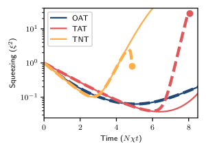
Figure 4: Spin squeezing throughout decoherence-free evolution of $N=100$ spins initially in the state $\ket{\text{X}}$, computed using both exact methods (solid lines) and the TST expansion in Eq. (10) with $M=35$ (dashed lines). Solid circles mark the times at which the TST expansion gives an unphysical result with $\xi^{2}<0$.

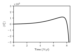
Figure 5: A collective spin correlator in the TAT model with $N=100$ spins and no decoherence, computed using the TST expansion with $M=35$. The divergence of correlators of this sort can be used to diagnose the breakdown of the TST expansion.

Appendix M Spin squeezing with strong decoherence

Here we provide supplementary evidence of our finding in Section III that the TNT model can produce more squeezing than the OAT or TAT models in the presence of strong decoherence. To this end, Figure 6 shows the minimal squeezing parameter $\xi^{2}_{\text{min}}$ achievable with $N=100$ spins through the OAT, TAT, and TNT models as a function of the rate $\gamma_{0}$ at which individual spins undergo spontaneous decay, excitation, and dephasing. These results were computed with quantum trajectory simulations, with $10^{3}$ trajectories per data point. While the OAT and TAT models produce more squeezing than the TNT model with weak decoherence, this squeezing falls off faster with an increasing decoherence rate $\gamma_{0}$. The relative robustness of TNT is in part a consequence of the fact that TNT initially generates squeezing at a faster rate than OAT or TAT, thereby allowing it to produce more squeezing before the degrading effects of decoherence kick in.

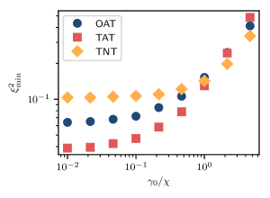
Figure 6: Optimal spin squeezing of $N=100$ spins undergoing spontaneous decay, excitation, and dephasing at rates $\gamma_{-}=\gamma_{+}=\gamma_{\text{z}}=\gamma_{0}$, computed using quantum trajectory simulations with $10^{3}$ trajectories per data point.

Appendix N Heisenberg operators in open quantum systems

Here we explain the origin and character of the mean-zero “noise” operators $\mathcal{E}_{\mathcal{O}}\left(t\right)$ that appear in the expansion of a Heisenberg operator $\mathcal{O}\left(t\right)=\sum_{\bm{m}}\mathcal{O}_{\bm{m}}\left(t\right)\mathcal{S}_{\bm{m}}+\mathcal{E}_{\mathcal{O}}\left(t\right)$ with time-dependent coefficients $\mathcal{O}_{\bm{m}}\left(t\right)$ for time-independent Schrödinger operators $\mathcal{S}_{\bm{m}}$. Our discussion should clarify why noise operators play no role in our calculation of expectation values of the form $\braket{\mathcal{O}\left(t\right)}$ and $\braket{\mathcal{O}\mathcal{Q}\left(t\right)}$, despite the fact that noise operators generally do need to be considered in the calculation of more general multi-time correlators in open quantum systemsBlocher and Mølmer (2019).

In any closed quantum system with initial state $\rho$ and propagator $U\left(t\right)$, such that the state at time $t$ is $\rho\left(t\right)\equiv U\left(t\right)\rho U^{\dagger}\left(t\right)$, time-dependent Heisenberg operators $\mathcal{O}\left(t\right)$ are uniquely defined from time-independent Schrödinger operators $\mathcal{O}$ by

$$\braket{\mathcal{O}\left(t\right)}\equiv\tr\left[\rho\left(t\right)\mathcal{O}\right]=\tr\left[\rho\mathcal{O}\left(t\right)\right].$$ (164)

Enforcing (164) for arbitrary initial states $\rho$ forces $\mathcal{O}\left(t\right)=U^{\dagger}\left(t\right)\mathcal{O}U\left(t\right)$. In an open quantum system, however, the definition of a Heisenberg operator is not so straightforward. Open systems can often be understood as subsystems of a larger closed system. Consider therefore an open system $S$ with environment $E$, a joint initial state $\rho_{SE}$, and propagator $U_{SE}\left(t\right)$. The reduced state $\rho_{S}\left(t\right)$ of $S$ at time $t$ is

$$\rho_{S}\left(t\right)\equiv\tr_{E}\left[\rho_{SE}\left(t\right)\right]=\tr_{E}\left[U_{SE}\left(t\right)\rho_{SE}U_{SE}^{\dagger}\left(t\right)\right]\equiv\mathcal{U}_{\underline{S}}\left(t\right)\rho_{S},$$ (165)

where $\rho_{S}\equiv\rho_{S}\left(0\right)$ is a time-independent state of $S$ in the Heisenberg picture, $\underline{S}$ denotes the space of operators on $S$, and the quantum channel $\mathcal{U}_{\underline{S}}\left(t\right)$ has the decompositionRivas and Huelga (2012)

$$\mathcal{U}_{\underline{S}}\left(t\right)\rho_{S}=\sum_{j}\mathcal{U}_{S}^{(j)}\left(t\right)\rho_{S}\mathcal{U}_{S}^{(j){\dagger}}\left(t\right)$$ (166)

with ordinary operators $\mathcal{U}_{S}^{(j)}\left(t\right)$ on $S$. We can therefore expand

$$\braket{\mathcal{O}_{S}\left(t\right)}=\tr\left[\rho_{S}\left(t\right)\mathcal{O}_{S}\right]=\tr\left[\mathcal{U}_{\underline{S}}\left(t\right)\rho_{S}\mathcal{O}_{S}\right]=\tr\left[\rho_{S}\mathcal{U}_{\underline{S}}^{\dagger}\left(t\right)\mathcal{O}_{S}\right]=\tr\left[\rho_{S}\underline{\mathcal{O}_{S}}\left(t\right)\right]=\braket{\underline{\mathcal{O}_{S}}\left(t\right)},$$ (167)

where $\mathcal{U}_{\underline{S}}^{\dagger}\left(t\right)$ is the adjoint map of $\mathcal{U}_{\underline{S}}\left(t\right)$ (with respect to a trace inner product between operators on $S$), and we define the time-dependent operator

$$\underline{\mathcal{O}_{S}}\left(t\right)\equiv\mathcal{U}_{\underline{S}}^{\dagger}\left(t\right)\mathcal{O}_{S}=\sum_{j}\mathcal{U}_{S}^{(j){\dagger}}\left(t\right)\mathcal{O}_{S}\mathcal{U}_{S}^{(j)}\left(t\right).$$ (168)

We thus find that substituting $\underline{\mathcal{O}_{S}}\left(t\right)$ in place of $\mathcal{O}_{S}\left(t\right)$ suffices for the calculation of correlators $\braket{\mathcal{O}_{S}\left(t\right)}$, thereby accounting for the validity of the equation of motion in (2). As we show below, this substitution also suffices for the calculation of two-time correlators of the form $\braket{\mathcal{O}_{S}\mathcal{Q}_{S}\left(t\right)}$ when the environment $E$ is Markovian.

The problem with defining Heisenberg operators $\mathcal{O}_{S}\left(t\right)$ by $\underline{\mathcal{O}_{S}}\left(t\right)$ only becomes evident when considering products of Heisenberg operators. One would like for the product of two Heisenberg operators $\mathcal{O}_{S}\left(t\right)$ and $\mathcal{Q}_{S}\left(t\right)$ to satisfy $\mathcal{O}_{S}\left(t\right)\mathcal{Q}_{S}\left(t\right)=\left(\mathcal{O}_{S}\mathcal{Q}_{S}\right)\left(t\right)$. This intuition can be formalized by observing that

$$\braket{\mathcal{O}_{S}\left(t\right)}=\tr\left[\rho_{SE}\left(t\right)\left(\mathcal{O}_{S}\otimes\mathds{1}_{E}\right)\right]=\tr\left[\rho_{SE}\left(\mathcal{O}_{S}\otimes\mathds{1}_{E}\right)\left(t\right)\right]=\braket{\left(\mathcal{O}_{S}\otimes\mathds{1}_{E}\right)\left(t\right)},$$ (169)

where $\mathds{1}_{E}$ is the identity operator on $E$, expectation values of Heisenberg operators on system $A\in\set{S,E,SE}$ are taken with respect to the state $\rho_{A}$, and

$$\left(\mathcal{O}_{S}\otimes\mathds{1}_{E}\right)\left(t\right)\equiv U_{SE}^{\dagger}\left(t\right)\left(\mathcal{O}_{S}\otimes\mathds{1}_{E}\right)U_{SE}\left(t\right).$$ (170)

By expanding Heisenberg operators similarly to (169) and (170), we then find

$$\braket{\mathcal{O}_{S}\left(t\right)\mathcal{Q}_{S}\left(t\right)}=\braket{\left(\mathcal{O}_{S}\otimes\mathds{1}_{E}\right)\left(t\right)\left(\mathcal{Q}_{S}\otimes\mathds{1}_{E}\right)\left(t\right)}=\braket{\left(\mathcal{O}_{S}\mathcal{Q}_{S}\otimes\mathds{1}_{E}\right)\left(t\right)}=\braket{\left(\mathcal{O}_{S}\mathcal{Q}_{S}\right)\left(t\right)}.$$ (171)

The expression in (168), however, makes it clear that generally $\underline{\mathcal{O}_{S}}\left(t\right)\underline{\mathcal{Q}_{S}}\left(t\right)\neq\left(\underline{\mathcal{O}_{S}\mathcal{Q}_{S}}\right)\left(t\right)$. To correct for this discrepancy, we define

$$\mathcal{O}_{S}\left(t\right)\equiv\underline{\mathcal{O}_{S}}\left(t\right)+\mathcal{E}_{\mathcal{O}_{S}}\left(t\right)$$ (172)

in terms of new “noise” operators $\mathcal{E}_{\mathcal{O}_{S}}\left(t\right)$ that are essentially defined to enforce the consistency of operator products such as $\mathcal{O}_{S}\left(t\right)\mathcal{Q}_{S}\left(t\right)=\left(\mathcal{O}_{S}\mathcal{Q}_{S}\right)\left(t\right)$. Self-consistency forces noise operators to be mean-zero, as

$$\braket{\mathcal{E}_{\mathcal{O}_{S}}\left(t\right)}=\braket{\mathcal{O}_{S}\left(t\right)}-\braket{\underline{\mathcal{O}_{S}}\left(t\right)}=0.$$ (173)

Furthermore, if the environment $E$ is Markovian, then noise operators are also uncorrelated with initial-time observables, i.e. $\braket{\mathcal{O}_{S}\mathcal{E}_{\mathcal{Q}_{S}}\left(t\right)}=0$, which means that noise operators can be neglected in the calculation of two-time correlators of the form $\braket{\mathcal{O}_{S}\mathcal{Q}_{S}\left(t\right)}$. To see why, we observe that a Markovian environment is essentially defined to satisfy

$$\rho_{SE}\left(t\right)=U_{SE}\left(t\right)\rho_{SE}U_{SE}^{\dagger}\left(t\right)\approx\rho_{S}\left(t\right)\otimes\rho_{E}=\mathcal{U}_{\underline{S}}\left(t\right)\rho_{S}\otimes\rho_{E},$$ (174)

with $\rho_{E}$ a time-independent steady state of the environment. If we enforce (174) for all states $\rho_{S}$, e.g. the maximally mixed state $\rho_{S}^{(1)}\propto\mathds{1}_{S}$ and $\rho_{S}^{(2)}\equiv\rho_{S}^{(1)}+\mathcal{O}_{S}$ with $\mathcal{O}_{S}$ any traceless operator on $S$ with operator norm $\mathinner{\!\left\lVert\mathcal{O}_{S}\right\rVert}\leq 1/\tr\mathds{1}_{S}$ (i.e. such that $\rho_{S}^{(2)}$ remains positive semi-definite, or a valid quantum state), then by linearity we find that

$$U_{SE}\left(t\right)\left(\mathds{1}_{S}\otimes\rho_{E}\right)U_{SE}^{\dagger}\left(t\right)\approx\mathcal{U}_{\underline{S}}\left(t\right)\mathds{1}_{S}\otimes\rho_{E}, U_{SE}\left(t\right)\left(\mathcal{O}_{S}\otimes\rho_{E}\right)U_{SE}^{\dagger}\left(t\right)\approx\mathcal{U}_{\underline{S}}\left(t\right)\mathcal{O}_{S}\otimes\rho_{E},$$ (175)

which implies that the Markov approximation (174) holds even if we replace $\rho_{S}$ by any operator on $S$, and in particular

$$U_{SE}\left(t\right)\rho_{SE}\left(\mathcal{O}_{S}\otimes\mathds{1}_{E}\right)U_{SE}^{\dagger}\left(t\right)=U_{SE}\left(t\right)\left(\rho_{S}\mathcal{O}_{S}\otimes\rho_{E}\right)U_{SE}^{\dagger}\left(t\right)\approx\mathcal{U}_{\underline{S}}\left(t\right)\left(\rho_{S}\mathcal{O}_{S}\right)\otimes\rho_{E}.$$ (176)

We can therefore expand

$$\braket{\mathcal{O}_{S}\mathcal{Q}_{S}\left(t\right)} =\tr\left[\rho_{SE}\left(\mathcal{O}_{S}\otimes\mathds{1}_{E}\right)U_{SE}^{\dagger}\left(t\right)\left(\mathcal{Q}_{S}\otimes\mathds{1}_{E}\right)U_{SE}\left(t\right)\right]$$ (177)

$$=\tr\left[U_{SE}\left(t\right)\rho_{SE}\left(\mathcal{O}_{S}\otimes\mathds{1}_{E}\right)U_{SE}^{\dagger}\left(t\right)\left(\mathcal{Q}_{S}\otimes\mathds{1}_{E}\right)\right],$$ (178)

and invoke the Markov approximation in (176) to find that

$$\braket{\mathcal{O}_{S}\mathcal{Q}_{S}\left(t\right)}\approx\tr\left[\mathcal{U}_{\underline{S}}\left(t\right)\left(\rho_{S}\mathcal{O}_{S}\right)\mathcal{Q}_{S}\right]=\tr\left[\rho_{S}\mathcal{O}_{S}\mathcal{U}_{\underline{S}}^{\dagger}\left(t\right)\mathcal{Q}_{S}\right]=\braket{\mathcal{O}_{S}\underline{\mathcal{Q}_{S}}\left(t\right)},$$ (179)

which implies

$$\braket{\mathcal{O}_{S}\mathcal{E}_{\mathcal{Q}_{S}}\left(t\right)}=\braket{\mathcal{O}_{S}\mathcal{Q}_{S}\left(t\right)}-\braket{\mathcal{O}_{S}\underline{\mathcal{Q}_{S}}\left(t\right)}\approx 0.$$ (180)

Noise operators thus play no role in the calculation of correlators such as $C\left(t\right)$ in (15). In contrast, noise operators generally do play a role in the calculation of multi-time correlators of the form $\braket{\prod_{j}\mathcal{O}_{S}^{(j)}\left(t_{j}\right)}$Blocher and Mølmer (2019). Furthermore, these calculations generally require additional assumptions about the environment. To keep our discussion simple and general, we therefore exclude the effects of noise terms in Section IV.

Appendix O Short-time linear response and two-time correlators

Here we discuss the appearance of two-time correlation functions in the short-time linear response of correlators to perturbations of a Hamiltonian. Consider an initial Hamiltonian $H$ perturbed by an operator $V$ with $\mathinner{\!\left\lVert V\right\rVert}\ll\mathinner{\!\left\lVert H\right\rVert}$, where $\mathinner{\!\left\lVert\mathcal{O}\right\rVert}$ denotes the operator norm of $\mathcal{O}$, such that the net Hamiltonian is $\tilde{H}=H+V$. We denote the generator of Heisenberg time evolution under the perturbed (unperturbed) Hamiltonian by $\tilde{T}$ ($T$). These generators are related by

$$\tilde{T}=T+i\underline{V}$$ (181)

where $\underline{V}$ is a superoperator whose action on operators $\mathcal{O}$ is defined by

$$\underline{V}\mathcal{O}\equiv\left[V,\mathcal{O}\right]_{-}.$$ (182)

Through quadratic order in the time $t$ and linear order in the perturbation $\underline{V}$, we can say that

$$e^{t\tilde{T}}\approx\dfrac{1}{2}\left[e^{tT},e^{it\underline{V}}\right]_{+}\approx e^{tT}+\dfrac{1}{2}it\left[e^{tT},\underline{V}\right]_{+}.$$ (183)

Defining perturbed and unperturbed Heisenberg operators $\tilde{\mathcal{O}}\left(t\right)$ and $\mathcal{O}\left(t\right)$ that respectively satisfy $\braket{\tilde{\mathcal{O}}\left(t\right)}=\braket{e^{t\tilde{T}}\mathcal{O}}$ and $\braket{\mathcal{O}\left(t\right)}=\braket{e^{tT}\mathcal{O}}$, we thus find that for sufficiently small times $t$ and weak perturbations $V$,

$$\braket{\tilde{\mathcal{O}}\left(t\right)-\mathcal{O}\left(t\right)}=\Braket{\left(e^{t\tilde{T}}-e^{tT}\right)\mathcal{O}}\approx\dfrac{1}{2}it\left(\braket{\left[V,\mathcal{O}\right]_{-}\left(t\right)}+\braket{\left[V,\mathcal{O}\left(t\right)\right]_{-}}\right).$$ (184)

Two-time correlators $\braket{V\mathcal{O}\left(t\right)}$ and $\braket{\mathcal{O}\left(t\right)V}$, in addition to the expectation values $\braket{\left(V\mathcal{O}\right)\left(t\right)}$ and $\braket{\left(\mathcal{O}V\right)\left(t\right)}$, thus determine the short-time linear response of correlators $\braket{\mathcal{O}\left(t\right)}$ to perturbations $V$ of a Hamiltonian.

References

- Dicke (1954) R. H. Dicke, Coherence in Spontaneous Radiation Processes, Physical Review 93, 99 (1954).
- Lipkin et al. (1965) H. J. Lipkin, N. Meshkov, and A. J. Glick, Validity of many-body approximation methods for a solvable model: (I). Exact solutions and perturbation theory, Nuclear Physics 62, 188 (1965).
- Meshkov et al. (1965) N. Meshkov, A. J. Glick, and H. J. Lipkin, Validity of many-body approximation methods for a solvable model: (II). Linearization procedures, Nuclear Physics 62, 199 (1965).
- Glick et al. (1965) A. J. Glick, H. J. Lipkin, and N. Meshkov, Validity of many-body approximation methods for a solvable model: (III). Diagram summations, Nuclear Physics 62, 211 (1965).
- Takano et al. (2009) T. Takano, M. Fuyama, R. Namiki, and Y. Takahashi, Spin Squeezing of a Cold Atomic Ensemble with the Nuclear Spin of One-Half, Physical Review Letters 102, 033601 (2009).
- Appel et al. (2009) J. Appel, P. J. Windpassinger, D. Oblak, U. B. Hoff, N. Kjærgaard, and E. S. Polzik, Mesoscopic atomic entanglement for precision measurements beyond the standard quantum limit, Proceedings of the National Academy of Sciences 106, 10960 (2009).
- Klinder et al. (2015) J. Klinder, H. Keßler, M. Wolke, L. Mathey, and A. Hemmerich, Dynamical phase transition in the open Dicke model, Proceedings of the National Academy of Sciences 112, 3290 (2015).
- Estève et al. (2008) J. Estève, C. Gross, A. Weller, S. Giovanazzi, and M. K. Oberthaler, Squeezing and entanglement in a Bose–Einstein condensate, Nature 455, 1216 (2008).
- Riedel et al. (2010) M. F. Riedel, P. Böhi, Y. Li, T. W. Hänsch, A. Sinatra, and P. Treutlein, Atom-chip-based generation of entanglement for quantum metrology, Nature 464, 1170 (2010).
- Gross et al. (2010) C. Gross, T. Zibold, E. Nicklas, J. Estève, and M. K. Oberthaler, Nonlinear atom interferometer surpasses classical precision limit, Nature 464, 1165 (2010).
- Martin et al. (2013) M. J. Martin, M. Bishof, M. D. Swallows, X. Zhang, C. Benko, J. von-Stecher, A. V. Gorshkov, A. M. Rey, and J. Ye, A Quantum Many-Body Spin System in an Optical Lattice Clock, Science 341, 632 (2013).
- Bromley et al. (2018) S. L. Bromley, S. Kolkowitz, T. Bothwell, D. Kedar, A. Safavi-Naini, M. L. Wall, C. Salomon, A. M. Rey, and J. Ye, Dynamics of interacting fermions under spin–orbit coupling in an optical lattice clock, Nature Physics 14, 399 (2018).
- Smale et al. (2019) S. Smale, P. He, B. A. Olsen, K. G. Jackson, H. Sharum, S. Trotzky, J. Marino, A. M. Rey, and J. H. Thywissen, Observation of a transition between dynamical phases in a quantum degenerate Fermi gas, Science Advances 5, eaax1568 (2019).
- Bohnet et al. (2016) J. G. Bohnet, B. C. Sawyer, J. W. Britton, M. L. Wall, A. M. Rey, M. Foss-Feig, and J. J. Bollinger, Quantum spin dynamics and entanglement generation with hundreds of trapped ions, Science 352, 1297 (2016).
- Schleier-Smith et al. (2010a) M. H. Schleier-Smith, I. D. Leroux, and V. Vuletić, States of an Ensemble of Two-Level Atoms with Reduced Quantum Uncertainty, Physical Review Letters 104, 073604 (2010a).
- Chen et al. (2011) Z. Chen, J. G. Bohnet, S. R. Sankar, J. Dai, and J. K. Thompson, Conditional Spin Squeezing of a Large Ensemble via the Vacuum Rabi Splitting, Physical Review Letters 106, 133601 (2011).
- Baumann et al. (2010) K. Baumann, C. Guerlin, F. Brennecke, and T. Esslinger, Dicke quantum phase transition with a superfluid gas in an optical cavity, Nature 464, 1301 (2010).
- Leroux et al. (2010) I. D. Leroux, M. H. Schleier-Smith, and V. Vuletić, Implementation of Cavity Squeezing of a Collective Atomic Spin, Physical Review Letters 104, 073602 (2010).
- Bohnet et al. (2014) J. G. Bohnet, K. C. Cox, M. A. Norcia, J. M. Weiner, Z. Chen, and J. K. Thompson, Reduced spin measurement back-action for a phase sensitivity ten times beyond the standard quantum limit, Nature Photonics 8, 731 (2014).
- Cox et al. (2016) K. C. Cox, G. P. Greve, J. M. Weiner, and J. K. Thompson, Deterministic Squeezed States with Collective Measurements and Feedback, Physical Review Letters 116, 093602 (2016).
- Hosten et al. (2016a) O. Hosten, N. J. Engelsen, R. Krishnakumar, and M. A. Kasevich, Measurement noise 100 times lower than the quantum-projection limit using entangled atoms, Nature 529, 505 (2016a).
- Hosten et al. (2016b) O. Hosten, R. Krishnakumar, N. J. Engelsen, and M. A. Kasevich, Quantum phase magnification, Science 352, 1552 (2016b).
- Norcia et al. (2018) M. A. Norcia, R. J. Lewis-Swan, J. R. K. Cline, B. Zhu, A. M. Rey, and J. K. Thompson, Cavity-mediated collective spin-exchange interactions in a strontium superradiant laser, Science 361, 259 (2018).
- Ritsch et al. (2013) H. Ritsch, P. Domokos, F. Brennecke, and T. Esslinger, Cold atoms in cavity-generated dynamical optical potentials, Reviews of Modern Physics 85, 553 (2013).
- Latorre et al. (2005) J. I. Latorre, R. Orús, E. Rico, and J. Vidal, Entanglement entropy in the Lipkin-Meshkov-Glick model, Physical Review A 71, 064101 (2005).
- Alcalde et al. (2007) M. A. Alcalde, A. L. L. de Lemos, and N. F. Svaiter, Functional methods in the generalized Dicke model, Journal of Physics A: Mathematical and Theoretical 40, 11961 (2007).
- Wang et al. (2012) C. Wang, Y.-Y. Zhang, and Q.-H. Chen, Quantum correlations in collective spin systems, Physical Review A 85, 052112 (2012).
- Majd et al. (2014) N. Majd, J. Payamara, and F. Daliri, LMG model: Markovian evolution of classical and quantum correlations under decoherence, The European Physical Journal B 87, 49 (2014).
- Walls et al. (1978) D. F. Walls, P. D. Drummond, S. S. Hassan, and H. J. Carmichael, Non-Equilibrium Phase Transitions in Cooperative Atomic Systems, Progress of Theoretical Physics Supplement 64, 307 (1978).
- Morrison and Parkins (2008a) S. Morrison and A. S. Parkins, Dynamical Quantum Phase Transitions in the Dissipative Lipkin-Meshkov-Glick Model with Proposed Realization in Optical Cavity QED, Physical Review Letters 100, 040403 (2008a).
- Morrison and Parkins (2008b) S. Morrison and A. S. Parkins, Dissipation-driven quantum phase transitions in collective spin systems, Journal of Physics B: Atomic, Molecular and Optical Physics 41, 195502 (2008b).
- Morrison and Parkins (2008c) S. Morrison and A. S. Parkins, Collective spin systems in dispersive optical cavity QED: Quantum phase transitions and entanglement, Physical Review A 77, 043810 (2008c).
- Kessler et al. (2012) E. M. Kessler, G. Giedke, A. Imamoglu, S. F. Yelin, M. D. Lukin, and J. I. Cirac, Dissipative phase transition in a central spin system, Physical Review A 86, 012116 (2012).
- Bhattacherjee (2014) A. B. Bhattacherjee, Non-equilibrium dynamical phases of the two-atom Dicke model, Physics Letters A 378, 3244 (2014).
- Zhiqiang et al. (2017) Z. Zhiqiang, C. H. Lee, R. Kumar, K. J. Arnold, S. J. Masson, A. S. Parkins, and M. D. Barrett, Nonequilibrium phase transition in a spin-1 Dicke model, Optica 4, 424 (2017).
- Lang et al. (2018) J. Lang, B. Frank, and J. C. Halimeh, Concurrence of dynamical phase transitions at finite temperature in the fully connected transverse-field Ising model, Physical Review B 97, 174401 (2018).
- Wineland et al. (1992) D. J. Wineland, J. J. Bollinger, W. M. Itano, F. L. Moore, and D. J. Heinzen, Spin squeezing and reduced quantum noise in spectroscopy, Physical Review A 46, R6797 (1992).
- Kitagawa and Ueda (1993) M. Kitagawa and M. Ueda, Squeezed spin states, Physical Review A 47, 5138 (1993).
- Zhong (2010) Z.-R. Zhong, A simplified scheme for realizing multi-atom NOON state, Optics Communications 283, 189 (2010).
- Schleier-Smith et al. (2010b) M. H. Schleier-Smith, I. D. Leroux, and V. Vuletić, Squeezing the collective spin of a dilute atomic ensemble by cavity feedback, Physical Review A 81, 021804(R) (2010b).
- Ma et al. (2011) J. Ma, X. Wang, C. P. Sun, and F. Nori, Quantum spin squeezing, Physics Reports 509, 89 (2011).
- Huang et al. (2015a) W. Huang, Y.-L. Zhang, C.-L. Zou, X.-B. Zou, and G.-C. Guo, Two-axis spin squeezing of two-component Bose-Einstein condensates via continuous driving, Physical Review A 91, 043642 (2015a).
- Muessel et al. (2015) W. Muessel, H. Strobel, D. Linnemann, T. Zibold, B. Juliá-Díaz, and M. K. Oberthaler, Twist-and-turn spin squeezing in Bose-Einstein condensates, Physical Review A 92, 023603 (2015).
- Huang et al. (2015b) J. Huang, X. Qin, H. Zhong, Y. Ke, and C. Lee, Quantum metrology with spin cat states under dissipation, Scientific Reports 5, 17894 (2015b).
- Hu et al. (2017) J. Hu, W. Chen, Z. Vendeiro, A. Urvoy, B. Braverman, and V. Vuletić, Vacuum spin squeezing, Physical Review A 96, 050301 (2017).
- Mirkhalaf et al. (2018) S. S. Mirkhalaf, S. P. Nolan, and S. A. Haine, Robustifying twist-and-turn entanglement with interaction-based readout, Physical Review A 97, 053618 (2018).
- Lewis-Swan et al. (2018) R. J. Lewis-Swan, M. A. Norcia, J. R. K. Cline, J. K. Thompson, and A. M. Rey, Robust Spin Squeezing via Photon-Mediated Interactions on an Optical Clock Transition, Physical Review Letters 121, 070403 (2018).
- He et al. (2019) P. He, M. A. Perlin, S. R. Muleady, R. J. Lewis-Swan, R. B. Hutson, J. Ye, and A. M. Rey, Engineering spin squeezing in a 3D optical lattice with interacting spin-orbit-coupled fermions, Physical Review Research 1, 033075 (2019).
- Itano et al. (1993) W. M. Itano, J. C. Bergquist, J. J. Bollinger, J. M. Gilligan, D. J. Heinzen, F. L. Moore, M. G. Raizen, and D. J. Wineland, Quantum projection noise: Population fluctuations in two-level systems, Physical Review A 47, 3554 (1993).
- Agarwal et al. (1997) G. S. Agarwal, R. R. Puri, and R. P. Singh, Atomic Schr\”odinger cat states, Physical Review A 56, 2249 (1997).
- Lau et al. (2014) H. W. Lau, Z. Dutton, T. Wang, and C. Simon, Proposal for the Creation and Optical Detection of Spin Cat States in Bose-Einstein Condensates, Physical Review Letters 113, 090401 (2014).
- Zwierz et al. (2010) M. Zwierz, C. A. Pérez-Delgado, and P. Kok, General Optimality of the Heisenberg Limit for Quantum Metrology, Physical Review Letters 105, 180402 (2010).
- Hu et al. (2015) J. Hu, W. Chen, Z. Vendeiro, H. Zhang, and V. Vuletić, Entangled collective-spin states of atomic ensembles under nonuniform atom-light interaction, Physical Review A 92, 063816 (2015).
- Hartmann (2016) S. Hartmann, Generalized Dicke States, Quantum Information and Computation 16, 16 (2016).
- Xu et al. (2013) M. Xu, D. A. Tieri, and M. J. Holland, Simulating open quantum systems by applying SU(4) to quantum master equations, Physical Review A 87, 062101 (2013).
- Plenio and Knight (1998) M. B. Plenio and P. L. Knight, The quantum-jump approach to dissipative dynamics in quantum optics, Reviews of Modern Physics 70, 101 (1998).
- Zhang et al. (2018) Y. Zhang, Y.-X. Zhang, and K. Mølmer, Monte-Carlo simulations of superradiant lasing, New Journal of Physics 20, 112001 (2018).
- Meiser and Holland (2010) D. Meiser and M. J. Holland, Steady-state superradiance with alkaline-earth-metal atoms, Physical Review A 81, 033847 (2010).
- Mori (1965) H. Mori, A Continued-Fraction Representation of the Time-Correlation Functions, Progress of Theoretical Physics 34, 399 (1965).
- Annett et al. (1994) J. F. Annett, W. Matthew, C. Foulkes, and R. Haydock, A recursive solution of Heisenberg’s equation and its interpretation, Journal of Physics: Condensed Matter 6, 6455 (1994).
- Liu et al. (2011) Y. C. Liu, Z. F. Xu, G. R. Jin, and L. You, Spin Squeezing: Transforming One-Axis Twisting into Two-Axis Twisting, Physical Review Letters 107, 013601 (2011).
- Micheli et al. (2003) A. Micheli, D. Jaksch, J. I. Cirac, and P. Zoller, Many-particle entanglement in two-component Bose-Einstein condensates, Physical Review A 67, 013607 (2003).
- Sorelli et al. (2019) G. Sorelli, M. Gessner, A. Smerzi, and L. Pezzè, Fast and optimal generation of entanglement in bosonic Josephson junctions, Physical Review A 99, 022329 (2019).
- Foss-Feig et al. (2013) M. Foss-Feig, K. R. A. Hazzard, J. J. Bollinger, and A. M. Rey, Nonequilibrium dynamics of arbitrary-range Ising models with decoherence: An exact analytic solution, Physical Review A 87, 042101 (2013).
- Blocher and Mølmer (2019) P. D. Blocher and K. Mølmer, Quantum regression theorem for out-of-time-ordered correlation functions, Physical Review A 99, 033816 (2019).
- Tucker et al. (2018) K. Tucker, B. Zhu, R. J. Lewis-Swan, J. Marino, F. Jimenez, J. G. Restrepo, and A. M. Rey, Shattered time: Can a dissipative time crystal survive many-body correlations?, New Journal of Physics 20, 123003 (2018).
- Maldacena et al. (2016) J. Maldacena, S. H. Shenker, and D. Stanford, A bound on chaos, Journal of High Energy Physics 2016, 106 (2016).
- Swingle (2018) B. Swingle, Unscrambling the physics of out-of-time-order correlators, Nature Physics 14, 988 (2018).
- García-Mata et al. (2018) I. García-Mata, M. Saraceno, R. A. Jalabert, A. J. Roncaglia, and D. A. Wisniacki, Chaos Signatures in the Short and Long Time Behavior of the Out-of-Time Ordered Correlator, Physical Review Letters 121, 210601 (2018).
- Note (1) In retrospect, it may have been nicer to push all operators to the right throughout these calculations, due to the enhanced symmetry that expressions would have with respect to Hermitian conjugation. In any case, we provide the final result of this section in both ordering conventions, and therefore feel no need to reproduce these calculations with a different ordering of spin operators.
- Rivas and Huelga (2012) A. Rivas and S. F. Huelga, Time Evolution in Open Quantum Systems, in Open Quantum Systems: An Introduction, SpringerBriefs in Physics, edited by A. Rivas and S. F. Huelga (Springer Berlin Heidelberg, Berlin, Heidelberg, 2012) pp. 19–31.