Quantum phase-sensitive diffraction and imaging using entangled photons

Abstract

We propose a novel quantum diffraction imaging technique whereby one photon of an entangled pair is diffracted off a sample and detected in coincidence with its twin. The image is obtained by scanning the photon that did not interact with matter. We show that when a dynamical quantum system interacts with an external field, the phase information is imprinted in the state of the field in a detectable way. The contribution to the signal from photons that interact with the sample scales as $\propto I_{p}^{\nicefrac{{1}}{{2}}}$, where $I_{p}$ is the source intensity, compared to $\propto I_{p}$ of classical diffraction. This makes imaging with weak-field possible, avoiding damage to delicate samples. A Schmidt decomposition of the state of the field can be used for image enhancement by reweighting the Schmidt modes contributions.

Rapid advances in short-wavelength ultrafast light sources, have revolutionized our ability to observe the microscopic world. With bright Free Electron Lasers and high harmonics tabletop sources, short time (femtosecond) and length (subnanometer) scales become accessible experimentally. These offer new exciting possibilities to study spatio-spectral properties of quantum systems driven out of equilibrium, and monitor dynamical relaxation processes and chemical reactions. The spatial features of small-scale charge distributions can be recorded in time. Far-field off-resonant X-ray diffraction measurements provide useful information on the charge density $\sigma\left(\boldsymbol{Q}\right)$ where $\boldsymbol{Q}$ is the diffraction wavector. The observed diffraction pattern $S\left(\boldsymbol{Q}\right)$ is given by the modulus square $S\left(\boldsymbol{Q}\right)\propto\left|\sigma\left(\boldsymbol{Q}\right)\right|^{2}$. Inverting these signals to real-space $\sigma\left(\boldsymbol{r}\right)$ requires a Fourier transform. Since the phase of $\sigma\left(\boldsymbol{Q}\right)$ is not available, the inversion requires phase retrieval which can be done using either algorithmic solutions Elser (2003); Fienup (1982) or more sophisticated and costly experimental setups such as heterodyne measurements Marx et al. (2008). Correlated beam techniques Walborn et al. (2010); Erkmen and Shapiro (2010); Gatti et al. (2004); Howell et al. (2004); Edgar et al. (2012); Aspden et al. (2013); Lemos et al. (2014) in the visible regime, have been shown to circumvent this problem by producing the real-space image of mesoscopic objects. Such techniques have classical analogues using correlated light, and reveal the modulus square of the studied object $\left|\sigma\left(\boldsymbol{r}\right)\right|^{2}$ Shapiro (2008); Bennink et al. (2002).

In this paper we consider the setup shown in Fig.$\left(\text{\ref{The setup}}\right)$. We focus on off-resonant scattering of entangled photons in which only one photon, denoted as the "signal", interacts with a sample. Its entangled counterpart, the "idler", is spatially scanned and measured in coincidence with the arrival of the signal photon. The idler reveals the image and also uncovers phase information, as was recently shown in Dorfman et al. (2019) for linear diffraction.

Our first main result is that for small diffraction angles, using Schmidt decomposition of the two-photon amplitude $\Phi\left(\boldsymbol{q}_{s},\boldsymbol{q}_{i}\right)=\sum_{n}^{\infty}\sqrt{\lambda_{n}}u_{n}\left(\boldsymbol{q}_{s}\right)v_{n}\left(\boldsymbol{q}_{i}\right)$ where $\lambda_{n}$ is the respective mode weight - reads,

$${\cal S}^{\left(p\right)}\left[\bar{\boldsymbol{\rho}}_{i}\right]\propto\mathfrak{Re}\sum_{nm}\sqrt{\lambda_{n}\lambda_{m}}\beta_{nm}^{\left(p\right)}v_{n}^{*}\left(\boldsymbol{\bar{\rho}}_{i}\right)v_{m}\left(\boldsymbol{\bar{\rho}}_{i}\right).$$ (1)

Here $\beta_{nm}^{\left(1\right)}=\int d\boldsymbol{r\>}u_{n}\left(\boldsymbol{r}\right)\sigma\left(\boldsymbol{r}\right)u_{m}^{*}\left(\boldsymbol{r}\right)$, $\beta_{nm}^{\left(2\right)}=\int d\boldsymbol{r\>}u_{n}\left(\boldsymbol{r}\right)\left|\sigma\left(\boldsymbol{r}\right)\right|^{2}u_{m}^{*}\left(\boldsymbol{r}\right)$ and $\boldsymbol{\bar{\rho}}_{i}$ represents the transverse detection plane. $\sigma\left(\boldsymbol{r}\right)$ is the charge density of the target object prepared by an actinic pulse and $p=\left(1,2\right)$ represents the order in $\sigma\left(\boldsymbol{r}\right)$. For large diffraction angels and frequency-resolved signal, the phase dependent image is modified to ${\cal S}\left[\bar{\boldsymbol{\rho}}_{i}\right]\propto\mathfrak{Re}\sum_{nm}^{\infty}\gamma_{nm}\sqrt{\lambda_{n}\lambda_{m}}v_{n}^{*}\left(\boldsymbol{\bar{\rho}}_{i}\right)v_{m}\left(\boldsymbol{\bar{\rho}}_{i}\right)$, where $\gamma_{nm}$ have a similar structure to $\beta_{nm}^{\left(1\right)}$ modulated by the Fourier decomposition of the Schmidt basis. $\gamma_{nm}$ is phase dependent in contrast to diffraction with classical sources.

Our second main result tackles the spatial resolution enhancement. In entanglement-based imaging, the resolution is limited by the degree of correlation of the two beams. Schmidt decomposition of the image allows to enhance desired spatial features of the charge density. High order Schmidt modes (which correspond to angular momentum transverse modes with high topological charge) offer more detailed matter information. Reweighting of Schmidt modes maximizes modal entropy which yields matter information gain and reveals fine details of the charge density. Moreover, ${\cal S}^{\left(1\right)}$ in Eq.$\left(\text{\ref{eq: small angel main eq}}\right)$ has no classical analogue, the contribution to the over-all signal from the "signal" photons scales as ${I}_{p}^{\nicefrac{{1}}{{2}}}$ where ${I}_{p}$ is the intensity of the source. This is a unique signature of the linear diffraction Dorfman et al. (2019). The over-all detected signal is obtained in coincidence and scales as $\propto{I}_{p}^{\nicefrac{{3}}{{2}}}$. Classical diffraction in contrast requires two interactions with the incoming field and therefore scales as $I_{p}$, and the corresponding coincidence scales as $\propto{I}_{p}^{2}$, which also applies for ${\cal S}^{\left(2\right)}$. Thanks to this favorable scaling, weak fields can be used to study fragile samples in order to avoid damage.

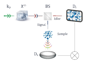
Figure 1: Sketch of the proposed quantum imaging setup. A broad-band pump $\boldsymbol{k}_{p}$ propagates through a $\chi^{\left(2\right)}$ crystal, generating an entangled photon pair denoted as signal and idler. The photons are distinguished either by polarization (type-II) or frequency (type-I) and are separated by a beam-splitter (BS). The signal photon interacts with the sample, and can be further frequency dispersed and collected by a ’bucket’ detector $D_{s}$ with no spatial resolution. The idler is spatially resolved in the transverse plane by the detector $D_{i}$. The two photons are detected in coincidence as defined in Eq.$\left(\text{\ref{eq: intensity-intensity definition}}\right)$.

I Spatial entanglement

Various sources of entangled photons are available, from quantum dots Huber et al. (2017), to cold atomic gasses Liang et al. (2018) and nonlinear crystals which are reviewed in Walborn et al. (2010). A general two-photon state can be written in the form,

$$|\psi\rangle=\sum_{\boldsymbol{k}_{s},\boldsymbol{k}_{i}}\Phi\left(\boldsymbol{k}_{s},\boldsymbol{k}_{i}\right)\epsilon_{\boldsymbol{k}_{s}}^{\left(\mu_{s}\right)}\epsilon_{\boldsymbol{k}_{i}}^{\left(\mu_{i}\right)}a_{\boldsymbol{k}_{s},\mu_{s}}^{\dagger}a_{\boldsymbol{k}_{i},\mu_{i}}^{\dagger}|0_{s},0_{i}\rangle,$$ (2)

where $\epsilon_{\boldsymbol{k}}^{\left(\nu\right)}$ is polarization, $a_{\boldsymbol{k,\nu}}\left(a_{\boldsymbol{k},\nu}^{\dagger}\right)$ are field annihilation (creation) operators and $\Phi\left(\boldsymbol{k}_{s},\boldsymbol{k}_{i}\right)$ is two photon amplitude. In the paraxial approximation the transverse momentum $\left\{\boldsymbol{q}_{s},\boldsymbol{q}_{i}\right\}$ and the longitudinal degrees of freedom are factorized. The transverse amplitude of photon-pair generated using parametric down converter takes then the form, Hong and Mandel (1985); Walborn et al. (2010); Grice and Walmsley (1997); Schlawin and Mukamel (2013),

$$\Phi\left(\boldsymbol{q}_{s},\boldsymbol{q}_{i}\right)=\Gamma\left(\boldsymbol{q}_{s}+\boldsymbol{q}_{i}\right)\text{sinc}\left(L^{2}\left(\boldsymbol{q}_{s}-\boldsymbol{q}_{i}\right)^{2}\right),$$ (3)

here $\Gamma\left(\boldsymbol{q}\right)$ are the pump envelope of the transverse components, $L^{2}=\nicefrac{{l_{z}\lambda_{p}}}{{4\pi}}$ where $\lambda_{p}$ is the central frequency wavelength and $l_{z}$ is the length of the nonlinear crystal along the longitudinal direction. The state of field is then given by,

$$|\psi\rangle =|\text{vac}\rangle+C\sum_{\begin{array}[]{c}\boldsymbol{q}_{s},\boldsymbol{q}_{i}\\ \omega_{s},\omega_{i}\end{array}}A_{p}\left(\omega_{s}+\omega_{i}\right)\Phi\left(\boldsymbol{q}_{s},\boldsymbol{q}_{i}\right)$$ (6)

$$\times|\boldsymbol{q}_{s},\omega_{s};\boldsymbol{q}_{i},\omega_{i}\rangle,$$ (7)

where $C$ is a normalization prefactor and $A_{p}$ is the pump envelope.

I.1 Schmidt decomposition of entangled two-photon states

The hallmark of entangled photon pairs is that they cannot be considered as two separate entities. This is expressed by the inseparability of the field amplitude $\Phi$ into a product of single photon amplitude; all the interesting quantum optical effects discussed below are derivatives of this feature. $\Phi$ can be represented as a superposition of separable states using the Schmidt decomposition Peres (1995); Ekert and Knight (1995); Law and Eberly (2004).

$$\Phi\left(\boldsymbol{q}_{s},\boldsymbol{q}_{i}\right)=\sum_{n}^{\infty}\sqrt{\lambda_{n}}u_{n}\left(\boldsymbol{q}_{s}\right)v_{n}\left(\boldsymbol{q}_{i}\right),$$ (8)

where the Schmidt modes $u_{n}\left(\boldsymbol{q}_{s}\right)$ and $v_{n}\left(\boldsymbol{q}_{i}\right)$ are the eigenvectors of the signal and the idler reduced density matrices, and the eigenvalues $\lambda_{n}$ satisfy the normalization $\sum_{n}\lambda_{n}=1$ Ekert and Knight (1995). The number of relevant modes serves as an indicator for the degree of inseparability of the amplitude, i.e. photon entanglement. Common measures for entanglement include the entropy $S_{ent}=-\sum_{n}\lambda_{n}\log_{2}\lambda_{n}$, or the Schmidt number $\kappa^{-1}\equiv\sum_{n}\lambda_{n}^{2}$. The latter is also known as the participation ratio as it quantifies the number of important Schmidt modes, or the effective joint Hilbert space size of the two photons. In a maximally entangled wavefunction, all modes contribute equally.

The spatial profile of the photons in the transverse plane (perpendicular to the propagation direction), can be expanded and measured using a variety of basis functions. E.g. Laguerre-Gauss (LG) or Hermite-Gauss (HG) have been demonstrated experimentally Mair et al. (2001); Straupe et al. (2011). These sets satisfy orthonormality $\int d^{2}\boldsymbol{q}\>u_{n}\left(\boldsymbol{q}\right)v_{k}\left(\boldsymbol{q}\right)=\delta_{nk}$ and closure relations $\sum_{n}\>u_{n}\left(\boldsymbol{q}\right)v_{n}\left(\boldsymbol{q}^{{}^{\prime}}\right)=\delta^{\left(2\right)}\left(\boldsymbol{q}-\boldsymbol{q}^{{}^{\prime}}\right)$. The deviation of $\lambda_{n}$ from a uniform (flat) distribution reflects the degree of entanglement. Perfect quantum correlations correspond to maximal entanglement entropy and thus a flat distribution of modes. This is further clarified by the closure relations, which demonstrate the convergence into a point-to-point mapping in the limit of perfect transverse entanglement. The biphoton amplitude has two limiting cases for infinite participation ratio which are demonstrated in Fig.$\left(\ref{fig:Schmidt-numbermVs. Amplitude}\right)$. When the sinc function in Eq.$\left(\text{\ref{eq:Amplitude 2D}}\right)$ is approximated by a Gaussian, the Schmidt number is given in a closed form Giedke et al. (2003),

$$\kappa=\frac{1}{4}\left(\sigma_{p}L+\frac{1}{\sigma_{p}L}\right)^{2},$$ (9)

where $\sigma_{p}^{2}$ is the variance of the transverse momentum of the pump. For $\sigma_{p}=l=1$, we get $\kappa=1$ and the two-photon wavefunction is separable $\Phi^{\left(\kappa=1\right)}\equiv\Phi^{\left(1\right)}\left(\boldsymbol{q}_{s},\boldsymbol{q}_{i}\right)=\Phi\left(\boldsymbol{q}_{s}\right)\Phi\left(\boldsymbol{q}_{i}\right)$ (no entanglement). A high number of relevant Schmidt modes indicates stronger quantum correlations between the two photons as shown in Fig.$\left(\ref{fig:Schmidt-numbermVs. Amplitude}\right)$. In the extreme cases of either vanishing or infinite product $\sigma_{p}l$ the photons are maximally entangled $\kappa\rightarrow\infty$, and the corresponding amplitude is $\Phi^{\left(\infty\right)}\left(\boldsymbol{q}_{s},\boldsymbol{q}_{i}\right)\propto\delta\left(\boldsymbol{q}_{s}\pm\boldsymbol{q}_{i}\right)$ as depicted in Fig.$\left(\ref{fig:Schmidt-numbermVs. Amplitude}\right)$. We denote by $\boldsymbol{\rho}_{s/i}$ the real-space transverse plane coordinate, conjugate to $\boldsymbol{q}_{s/i}$ . The real-space amplitude has two limiting cases, when $\sigma_{p}l\rightarrow 0$ $\Phi\left(\boldsymbol{\rho}_{s},\boldsymbol{\rho}_{i}\right)=\Phi_{\ll}^{\left(\infty\right)}\left(\boldsymbol{\rho}_{s},\boldsymbol{\rho}_{i}\right)=\Phi_{0}\delta\left(\boldsymbol{\rho}_{s}-\boldsymbol{\rho}_{i}\right)$. This amplitude maps the image plane explored by the signal photon directly into the idler’s detector. The opposite limiting case $\sigma_{p}L\rightarrow\infty$ is given by the amplitude $\Phi\left(\boldsymbol{\rho}_{s},\boldsymbol{\rho}_{i}\right)=\Phi_{\gg}^{\left(\infty\right)}\left(\boldsymbol{\rho}_{s},\boldsymbol{\rho}_{i}\right)=\Phi_{0}\delta\left(\boldsymbol{\rho}_{s}+\boldsymbol{\rho}_{i}\right)$. This amplitude maps the sample plane monitored by the signal photon $\boldsymbol{\rho}_{s}\rightarrow-\boldsymbol{\rho}_{i}$ which results in the mirror image. We use the abbreviated notation whereby $\bar{\boldsymbol{\rho}_{i}}$ denotes the mapping from the sample to the detector plane with the corresponding sign.

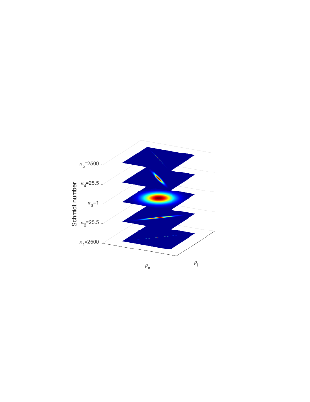
Figure 2: Transverse beam amplitude profile for different Schmidt Numbers. For $\kappa_{3}=1$ the amplitude in Eq.$\left(\text{\ref{eq:Schmidt decomposition}}\right)$ is separable and the photons are not entangled. As $\kappa$ is increased the amplitude approaches a narrow distribution. $\kappa_{1}=2500$ and $\kappa_{2}=25.5$ are obtained in the $\sigma_{p}L>1$ regime, the amplitude approaches $\Phi_{\gg}^{\left(\infty\right)}\propto\delta\left(\boldsymbol{q}_{s}+\boldsymbol{q}_{i}\right)$. $\kappa_{4}=25.5$ and $\kappa_{5}=2500$ are taken in the $\sigma_{p}L<1$ regime, with the asymptotic amplitude $\Phi_{\ll}^{\left(\infty\right)}\propto\delta\left(\boldsymbol{q}_{s}-\boldsymbol{q}_{i}\right)$.

II The reduced idler density matrix in the Schmidt basis

The reduced density matrix of the idler reveals the role of quantum correlations in the proposed detection measurement scheme [Fig.$\left(\ref{The setup}\right)$]. The joint light-matter density matrix in the interaction picture is given by,

$$\rho_{\mu\phi}^{int}\left(t\right)={\cal T}e^{-i\int d\tau{\cal H}_{I,-}\left(\tau\right)}\rho_{\mu}\otimes\rho_{\phi},$$ (10)

where ${\cal T}$ represents super-operator time ordering and the off-resonance radiation/matter coupling is ${\cal H}_{I}=\int d\boldsymbol{r}\sigma\left(\boldsymbol{r},t\right)\boldsymbol{A}^{2}\left(\boldsymbol{r},t\right)$ with the vector field $\boldsymbol{A}\left(\boldsymbol{r},t\right)=-\nicefrac{{\dot{\boldsymbol{E}}\left(\boldsymbol{r},t\right)}}{{c}}$. The subscript $\left(-\right)$ on a Hilbert space operators represents the commutator ${\cal O}_{-}\equiv\left[{\cal O},\cdot\right]$. The electric field is given by $\boldsymbol{E}\left(\boldsymbol{r},t\right)=\sum_{k}\boldsymbol{E}_{k}^{\left(+\right)}\left(\boldsymbol{r},t\right)+\boldsymbol{E}_{k}^{\left(-\right)}\left(\boldsymbol{r},t\right)$ such that,

$$\boldsymbol{E}_{k}^{\left(+\right)}\left(\boldsymbol{r},t\right)=\left(\boldsymbol{E}_{k}^{\left(-\right)}\left(\boldsymbol{r},t\right)\right)^{\dagger} =\sqrt{\frac{2\pi\hbar\omega_{\boldsymbol{k}}}{V_{\boldsymbol{k}}}}\sum_{\nu}\epsilon_{\boldsymbol{k}}^{\left(\nu\right)}a_{\boldsymbol{k},\nu}e^{i\boldsymbol{k}\cdot\boldsymbol{r}-i\omega_{\boldsymbol{k}}t},$$ (11)

$\mu$ stands for the matter’s degrees of freedom while $\phi$ represents the field’s degrees of freedom. For a weak field, one can expand the evolution of the density matrix in powers of the field which correspond to number of light-matter interactions. To first nontrivial order, a single interaction from the left or the right of the joint space density matrix corresponds to a change in the coherence in the field subspace $\rho_{\phi}=\text{tr}_{\mu}\rho_{\mu\phi}$. The radiation field records no photon exchange due to a single interaction with the matter, merely a change in its phase. When the initial state of the field contains an interesting internal structure such as quantum correlations arising from entanglement, the initial reduced density matrix $\rho_{\phi_{i}}=\text{tr}_{\mu\phi_{s}}\rho_{\mu,\phi_{si}}$ obtained by tracing over the signal beam is given by,

$$\rho_{\phi_{i}}\left(0\right)=\sum_{n,i,i^{\prime}}\lambda_{n}v_{n}^{*}\left(\boldsymbol{k}_{i}\right)v_{n}\left(\boldsymbol{k}_{i}^{\prime}\right)|\boldsymbol{1}_{i}\rangle\langle\boldsymbol{1}_{i^{\prime}}|,$$ (12)

which is diagonal in the idler subspace in the Schmidt basis. When the signal interacts with an external matter degree of freedom, the idler reduced density matrix is no longer diagonal. In the small diffraction angle limit it is given by (see appendix 1 of the SI),

$$\rho_{\phi_{i}}^{\left(1\right)}=\sum_{n,m,i,i^{\prime}}{\cal P}_{nm}v_{n}^{*}\left(\boldsymbol{k}_{i}\right)v_{m}\left(\boldsymbol{k}_{i}^{\prime}\right)|\boldsymbol{1}_{i}\rangle\langle\boldsymbol{1}_{i^{\prime}}|+h.c,$$ (13)

where ${\cal P}_{nm}=i\beta_{nm}^{\left(1\right)}\sqrt{\lambda_{n}\lambda_{m}}$, and,

$$\beta_{nm}^{\left(1\right)}=\int d\boldsymbol{r\>}u_{n}\left(\boldsymbol{r}\right)\sigma\left(\boldsymbol{r}\right)u_{m}^{*}\left(\boldsymbol{r}\right)$$ (14)

are the projections of matter quantities on the chosen Schmidt basis. Our setup allows to probe the induced coherence of the field due to its interaction with matter.

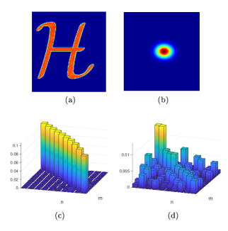
Figure 3: The reduced idler density-matrix in the Schmidt basis. $\left(a\right)$ The projected object. $\left(b\right)$ The ’spot-size’ corresponding to the $HG_{00}$ mode. $\left(c\right)$ The idler’s reduced density matrix before the interaction with the object presented in Hermite-Gauss basis modes, given by Eq.$\left(\ref{Density matrix before}\right)$. $\left(d\right)$ The change in the reduced density matrix of the idler due to the interaction with the object given by Eq. $\left(\text{\ref{eq: Density matrix after}}\right)$

Fig. $\left(\text{\ref{Reduced density matrix figures}}\right)$ displays the induced Schmidt-space coherence of the reduced density matrix of idler (the non-interacting photon) due to the interaction of its twin (signal) with an object. We have chosen the Hermite-Gauss basis, depicted in Fig.$\left(\text{\ref{fig:Hermite-Gaussian-modes visualization}}\right)$ for this visualization. Each mode is labeled by two indices, one for each spatial dimension of the image. In Fig.$\left(\text{\ref{Reduced density matrix figures}}.c,d\right)$, we have traced over the corresponding index, resulting in a one dimensional data set. Each coherence corresponds to a projection of the object between two modes. Eq.$\left(\text{\ref{eq: small angel main eq}}\right)$ can be derived as the intensity expectation value calculated from the idler’s reduced density matrix given in Eq.$\left(\text{\ref{eq: Density matrix after}}\right)$.

III Far-field diffraction

We next turn to far field diffraction with arbitrary scattering directions. While the incoming field is understood to be paraxial, the scattered field is not. The coincidence image in the far-field yields a similar expression to the one calculated from the reduced density matrix in Eq.$\left(\text{\ref{eq: Density matrix after}}\right)$ with an additional spatial phase factor characteristic to far-field diffraction. Using Eq.$\left(\ref{wave-function - general term}\right)$ for the setup described in Fig.$\left(\ref{The setup}\right)$, the coincidence image is given by the intensity-intensity correlation function (see SI),

$$S\left[\bar{\boldsymbol{\rho}}_{i}\right] =\int d\boldsymbol{X}_{s}d\boldsymbol{X}_{i}G_{s}\left(\boldsymbol{X}_{s},\bar{\boldsymbol{X}_{s}}\right)G_{i}\left(\boldsymbol{X}_{i},\bar{\boldsymbol{X}_{i}}\right)$$ (15)

$$\times\left\langle{\cal T}\hat{I}_{s}\left(\boldsymbol{r}_{s},t_{s}\right)\hat{I}_{i}\left(\boldsymbol{r}_{i},t_{i}\right){\cal U}_{I}\left(t\right)\right\rangle,$$

here $\hat{I}_{m}\left(\boldsymbol{r}_{m},t_{m}\right)\equiv\hat{\boldsymbol{E}}_{m,R}^{\left(-\right)}\left(\boldsymbol{r}_{m},t_{m}\right)\cdot\hat{\boldsymbol{E}}_{m,L}^{\left(+\right)}\left(\boldsymbol{r}_{m},t_{m}\right)$ are field intensity operators and $m=\left(s,i\right)$. The gating functions $G_{m}$ represent the details of the measurement process Glauber (2007); Roslyak and Mukamel (2009). Eq.$\left(\text{\ref{eq: intensity-intensity definition}}\right)$ can be calculated straight from the reduced density matrix of the idler, despite the fact that it includes the signal’s intensity operator. The reason stems from the fact that the intensity expectation value monitors the single photon space. The partial trace over a singly occupied signal state results in the same operation. Estimating this expression includes a 10 field operator correlation function which are shown explicitly in Eq(4) of appendix (2). In the far-field, upon rotational averaging we obtain (see appendix 2 of the SI),

$${\cal S} \left[\bar{\boldsymbol{\rho}}_{i}\right]\propto\mathfrak{Re}\int d\omega_{s}\mathscr{E}\left[\omega_{s}\right]\int d\boldsymbol{\rho}_{s}\Phi\left(\boldsymbol{\rho}_{s},\boldsymbol{\bar{\rho}}_{i}\right)\times$$

$$\int d\boldsymbol{\rho}^{{}^{\prime}}\Phi\left(\boldsymbol{\rho}^{{}^{\prime}},\bar{\boldsymbol{\rho}}_{i}\right)\boldsymbol{\boldsymbol{\sigma}}\left(\boldsymbol{\rho}^{{}^{\prime}}\right)e^{-i\boldsymbol{\boldsymbol{Q}_{s}}\cdot\boldsymbol{\rho}^{{}^{\prime}}}.$$ (16)

Here $\boldsymbol{Q}_{s}=\frac{\omega_{s}}{c}\hat{\rho}_{s}$ is the diffraction wavector, $\mathscr{E}\left[\omega_{s}\right]=\int d\omega_{i}G\left(\omega_{s}\right)G\left(\omega_{i}\right)\left|A\left(\omega_{s}+\omega_{i}\right)\right|^{2}$ is a functional of the frequency, ${\cal S}=-\left(S-S_{0}\right)$ is the image with the noninteracting-uniform background $\left(S_{0}\right)$ subtracted, and $\bar{\boldsymbol{\rho}}_{i}$ is the mapping coordinate onto the detector plane with the corresponding sign. $\boldsymbol{\boldsymbol{\sigma}}\left(\boldsymbol{\rho}\right)\equiv\sum_{\alpha;a,b}\left\langle a|\hat{\sigma}\left(\boldsymbol{\rho}-\boldsymbol{\rho}_{\alpha}\right)|b\right\rangle$ denotes a matrix element of the charge-density operator, traced over the longitudinal axis, with respect to the eigenstates $\left\{a,b\right\}$ and $\boldsymbol{\rho}_{\alpha}$ are positions of particles in the sample. The matter can be prepared initially in a superposition state. Substituting the Schmidt decomposition [Eq.$\left(\ref{eq:Schmidt decomposition}\right)$] into Eq.$\left(\ref{eq:Signal with general Phi-1-1}\right)$ gives,

$${\cal S} \left[\bar{\boldsymbol{\rho}}_{i}\right]\propto\mathfrak{Re}\int d\omega_{s}\mathscr{E}\left[\omega_{s}\right]d\boldsymbol{\rho}_{s}\sum_{nm}^{\infty}\sqrt{\lambda_{n}\lambda_{m}}u_{n}\left(\boldsymbol{\rho}_{s}\right)v_{n}^{*}\left(\boldsymbol{\bar{\rho}}_{i}\right)\times$$

$$v_{m}\left(\boldsymbol{\bar{\rho}}_{i}\right)\int d\boldsymbol{\rho}^{{}^{\prime}}u_{m}^{*}\left(\boldsymbol{\rho}^{{}^{\prime}}\right)\boldsymbol{\boldsymbol{\sigma}}\left(\boldsymbol{\rho}^{{}^{\prime}}\right)e^{-i\boldsymbol{Q}_{s}\cdot\boldsymbol{\rho}^{{}^{\prime}}}.$$ (17)

This shows a smooth transition from momentum to real space imaging. For low Schmidt modes that do not vary appreciably across the charge density scale, the last term yields $\boldsymbol{\boldsymbol{\sigma}}\left(\boldsymbol{Q}_{s}\right)\approx\int d\boldsymbol{\rho}^{{}^{\prime}}u_{m}^{*}\left(\boldsymbol{\rho}^{{}^{\prime}}\right)\boldsymbol{\boldsymbol{\sigma}}\left(\boldsymbol{\rho}^{{}^{\prime}}\right)e^{-i\boldsymbol{Q}_{s}\cdot\boldsymbol{\rho}^{{}^{\prime}}}$. Consequently, when the Schmidt modes do not vary on the lengthscale of the charge density up to high order, the Fourier decomposition of the charge density is projected on $u_{n}$ and reweights the corresponding idler modes. The resulting image given by spatial scanning of the idler is the Fourier transform of the charge density projected on the relevant idler mode. Alternately, when the Schmidt modes vary along the charge density, the exact expression for the far field diffraction image is given by,

$${\cal S}\left[\bar{\boldsymbol{\rho}}_{i}\right] \propto\mathfrak{Re}\sum_{nm}^{\infty}\gamma_{nm}\sqrt{\lambda_{n}\lambda_{m}}v_{n}^{*}\left(\boldsymbol{\bar{\rho}}_{i}\right)v_{m}\left(\boldsymbol{\bar{\rho}}_{i}\right)$$ (18)

$$\gamma_{nm} =\sum_{k}\beta_{km}^{\left(1\right)}\int d\boldsymbol{\rho}_{s}d\omega_{s}\mathscr{E}\left[\omega_{s}\right]u_{n}\left(\boldsymbol{\rho}_{s}\right)u_{k}^{*}\left(\boldsymbol{Q}_{s}\right),$$ (19)

where $\beta_{nm}^{\left(1\right)}$ was defined in Eq.$\left(\text{\ref{eq: Beta(1)}}\right)$. From the definition of $\boldsymbol{Q}_{s}$ it is evident that its angular component of $u_{k}$ is identical to the corresponding in $u_{n}$ and therefore $\gamma_{nm}$ is composed of summation over modes with the same angular momentum in the LG basis set.

It is also possible to calculate the real-space image of the charge density when the signal is frequency dispersed. Assuming for simplicity perfect quantum correlations between the signal and idler we obtain,

$${\cal S}\left[\bar{\boldsymbol{\rho}}_{i},\bar{\omega}_{s}\right]\propto\mathfrak{Re}\sigma\left(\boldsymbol{\bar{\rho}}_{i}\right)e^{-i\frac{\bar{\omega}_{s}}{c}\bar{\rho}_{i}}.$$ (20)

This image is phase dependent and unlike diffraction of classical light, allows to transform freely between momentum and real-space. The phase-dependent Fourier image in this limit is also given by resolving the signal photon with respect to the frequency $\bar{\omega}_{s}$ as well (see SI).

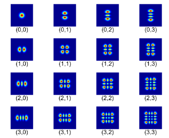
Figure 4: Hermite-Gaussian modes. Modes are labeled by two indices, each representing one dimension in the transverse plane.

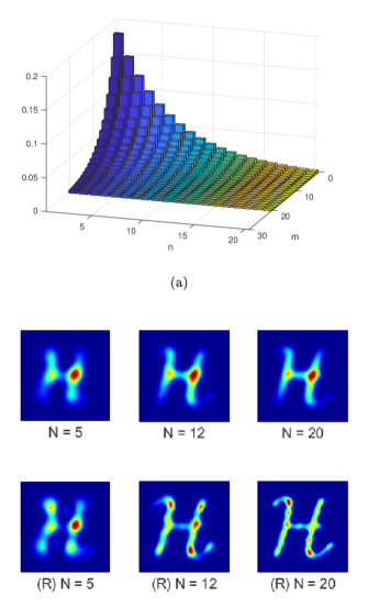
Figure 5: Weighted recombination of the truncated sum in Eq.$\left(\text{\ref{eq:projection}}\right)$, using HG basis with $\sigma_{p}l=0.07$, corresponding to $\kappa\approx 14$. $\left(a\right)$ Schmidt weights of the entangled light source. $\left(b\right)$ First order image. Recombination using the original weight of each mode (upper row), with respect to the $N$ first modes. This corresponds to straightforward imaging with the given parameters. The lower row shows the reweighted-flattened Schmidt spectrum recombination that corresponds to the $N$ first modes, marked with (R). $\left(c\right)$ The real part of the image $I\left(r,\phi\right)$ with added spatial phase $\left|I\left(\rho,\phi\right)\right|\exp\left[-i\frac{2\pi}{L/3}\rho\right]$. $\left(d\right)$ Reweighted truncated sum diffraction image given by Eq.$\left(\text{\ref{eq:projection}}\right)$ for N=20. Recovering the spatial phase.

IV Reweighted modal-contributions

The apparent classical-like form of the coherent superposition in the Schmidt representation, where each mode carries a distinct spatial matter information, suggests experiments in which a single Schmidt mode is measured at a time Straupe et al. (2011). This bares some resembles to the coherent mode representation of partially coherent sources studied in Wolf (1982); Vartanyants and Singer (2018). Moreover, it allows the reweighting of high angular momentum modes available experimentally Fickler et al. (2016), and known to have decreasing effect on the image upon naive summation. Reweighting of truncated sums is extensively used as sharpening tool in digital signal processing, especially in medical image enhancement Lehmann et al. (1999). This approach raises questions regarding the analysis of optimal Schmidt weights, error minimization and engineered functional decrease of weights as done in theory of sampled signals. The structure of the spatial information mapping from the signal to the idler takes a simpler form for small scattering angles. When we examine the first and second order contributions due to a single charge distribution, the resulting image of a truncated sum composed of the first $N$ modes is given by,

$${\cal S}_{N}^{\left(p\right)}\left[\bar{\boldsymbol{\rho}}_{i}\right] \propto\mathfrak{Re}\sum_{nm=0}^{N}\sqrt{\lambda_{n}\lambda_{m}}\beta_{nm}^{\left(p\right)}v_{n}^{*}\left(\boldsymbol{\bar{\rho}}_{i}\right)v_{m}\left(\boldsymbol{\bar{\rho}}_{i}\right),$$ (21)

where $\beta_{nm}^{\left(2\right)}=\int d\boldsymbol{r}\>u_{n}\left(\boldsymbol{r}\right)\left|\sigma\left(\boldsymbol{r}\right)\right|^{2}u_{m}^{*}\left(\boldsymbol{r}\right),$ is a scattering coefficient between Schmidt modes which resembles the expressions used in previous two-photon imaging techniques Shapiro (2008); Bennink et al. (2002); Walborn et al. (2010). $\beta_{nm}^{\left(1\right)}$ defined in Eq.$\left(\text{\ref{eq: Beta(1)}}\right)$, holds phase information of the studied object and have no classical counterpart. Its momentum space representation reads,

$$\beta_{nm}^{\left(1\right)}=\sum_{\boldsymbol{k}_{s},\boldsymbol{k}_{d}}u_{n}\left(\boldsymbol{k}_{s}\right)\sigma\left(\boldsymbol{k}_{s}-\boldsymbol{k}_{d}\right)u_{m}^{*}\left(\boldsymbol{k}_{d}\right)$$ (22)

where $d$ stands for a detected mode initially in a vacuum state. This shows more clearly the physical role played by the charge density in the coupling of different Schmidt modes.

Fig.$\left(\ref{fig:Weighted-recombination}a\right)$ presents the Schmidt spectrum for a beam characterized by $\sigma_{p}l=0.07$ which yields $\kappa\approx 14$. Fig.$\left(\ref{fig:Weighted-recombination}b\right)$ illustrates the improvement of the acquired image due to resummation of the Hermite-Gauss modes of the object decomposed in Fig. $\left(\text{\ref{Reduced density matrix figures}}\right)$. By using Eq.$\left(\text{\ref{eq:projection}}\right)$ with flattened Schmidt spectrum we demonstrate the enhancement of fine features of the diffracted image. Phase measurement is demonstrated in Fig.$\left(\ref{fig:Weighted-recombination}c,d\right)$.

V Discussion

The scattered quantum light from matter carries phase information at odd orders in the charge distribution $\sigma\left(\boldsymbol{q}\right)$ the light-matter interaction. To first order, the change in the quantum state of the field due to a single interaction is imprinted in the phase of the photons, which is detectable. However, no photon is generated in this order. Homodyne diffraction of classical sources results in even correlation functions of the charge density. We have provided a complete description of the charge distribution resulting from nonvanishing odd orders of the radiation-matter interaction. The detected image is sensitive to the degree of entanglement. High resolution is achieved in the limits of infinite or vanishing $\sigma_{p}l$, which are hard to realize. For a long nonlinear crystal, the phase matching factor is more dominant and strong beam divergence is required to generate strong quantum correlations. This limit is not compatible with the paraxial approximation for the amplitude and requires further study. In the short crystal limit the amplitude acquires the angular spectrum of the pump and the resolution is limited by the crystal length and low beam divergence.

We have demonstrated that coincidence diffraction measurements of entangled photons with quantum detection, can also achieve enhanced imaging resolution. Eq.$\left(\ref{eq:projection}\right)$ provides an intuitive picture for the information transfer from the signal to the idler beams. By reweighting the spatial modes that span the measured image, one can refine the matter information. High angular momentum states of light have been recently demonstrated experimentally with quantum numbers above $\sim 10^{4}$ Fickler et al. (2016). It is of cardinal practical importance to quantify the natural cutoff of high topologically charged modes in order to discuss sub-wavelength resolution. Reweighting the Schmidt modes distribution is motivated by the closure relations $\sum_{n}\>u_{n}\left(\boldsymbol{q}\right)v_{n}\left(\boldsymbol{q}^{{}^{\prime}}\right)=\delta^{\left(2\right)}\left(\boldsymbol{q}-\boldsymbol{q}^{{}^{\prime}}\right)$. This suggests that equal contribution of modes converges into a delta distribution of the two photon amplitude, perfectly transferring the spatial information between the photons. Finding optimal weights is a challenge for future studies. Signal acquisition optimization techniques used in sampling theory, avoiding high frequency quantization noise can be considered as well Lehmann et al. (1999).

The imaging of single localized biological molecules has been a major driving force for building free electron X-ray lasers Chapman et al. (2011). Such molecules are complex, fragile, and typically have multiple timescale dynamics. One strategy is to use a fresh sample in each iteration, assuming a destructive measurement. Ultra-short X-ray pulses have been proposed to reduce damage Neutzo et al. (2000). Entangled hard X-ray photons have been generated by parametric down conversion using a diamond crystal Shwartz et al. (2012). Avoiding damage of such complexes by using weak fields, allows to follow the evolution of initially perturbed charge densities. Linear diffraction scales as $\propto I_{p}^{\nicefrac{{1}}{{2}}}$ with the signal photons that interact with the sample while the over all coincidence image scales as $\propto I_{p}^{\nicefrac{{3}}{{2}}}$. Using diffraction of entangled photons from charge distributions initially prepared by ultrafast pulses, results in imaging of their real-space dynamics and provides a fascinating topic for future study.

Acknowledgments. The support of the Chemical Sciences, Geosciences, and Biosciences Division, Office of Basic Energy Sciences, Office of Science, U.S. Department of Energy is gratefully acknowledged. Collaborative visits of K.D. to UCI were supported by Award No. DEFG02-04ER15571 ,and. S.M was supported by Award DESC0019484. S.A fellowship was supported by the National Science Foundation (Grant No. CHE-1663822) . We also wish to thank Noa Asban for the graphical illustrations.

References

- Elser (2003) V. Elser, Phase retrieval by iterated projections, J. Opt. Soc. Am. A 20, 40 (2003).
- Fienup (1982) J. R. Fienup, Phase retrieval algorithms: a comparison, Appl. Opt. 21, 2758 (1982).
- Marx et al. (2008) C. A. Marx, U. Harbola, and S. Mukamel, Nonlinear optical spectroscopy of single, few, and many molecules: Nonequilibrium Green’s function QED approach, Phys. Rev. A 77, 22110 (2008).
- Walborn et al. (2010) S. P. Walborn, C. H. Monken, S. Pádua, and P. H. S. Ribeiro, Spatial correlations in parametric down-conversion, Physics Reports 495, 87 (2010), arXiv:1010.1236 .
- Erkmen and Shapiro (2010) B. I. Erkmen and J. H. Shapiro, Ghost imaging : from quantum to classical to computational, Advances in Optics and Photonics , 405 (2010).
- Gatti et al. (2004) A. Gatti, E. Brambilla, M. Bache, and L. A. Lugiato, Ghost Imaging with Thermal Light : Comparing Entanglement and Classical Correlation, Phys. Rev. Lett. , 1 (2004).
- Howell et al. (2004) J. C. Howell, R. S. Bennink, S. J. Bentley, and R. W. Boyd, Realization of the Einstein-Podolsky-Rosen Paradox Using Momentum- and Position-Entangled Photons from Spontaneous Parametric Down Conversion, Phys. Rev. Lett. , 1 (2004).
- Edgar et al. (2012) M. P. Edgar, D. S. Tasca, F. Izdebski, R. E. Warburton, J. Leach, M. Agnew, G. S. Buller, R. W. Boyd, and M. J. Padgett, Imaging high-dimensional spatial entanglement with a camera, Nature Communications 3, 984 (2012), arXiv:arXiv:1204.1293v2 .
- Aspden et al. (2013) R. S. Aspden, D. S. Tasca, R. W. Boyd, and M. J. Padgett, EPR-based ghost imaging using a single-photon-sensitive camera, New Journal of Physics 15, 10.1088/1367-2630/15/7/073032 (2013), arXiv:arXiv:1212.5059v2 .
- Lemos et al. (2014) G. B. Lemos, V. Borish, G. D. Cole, S. Ramelow, R. Lapkiewicz, and A. Zeilinger, Quantum imaging with undetected photons, Nature 512, 409 (2014).
- Shapiro (2008) J. H. Shapiro, Computational ghost imaging, Phys. Rev. A 78, 061802 (2008).
- Bennink et al. (2002) R. S. Bennink, S. J. Bentley, and R. W. Boyd, “two-photon” coincidence imaging with a classical source, Phys. Rev. Lett. 89, 113601 (2002).
- Dorfman et al. (2019) K. E. Dorfman, S. Asban, L. Ye, J. R. Rouxel, D. Cho, and S. Mukamel, Monitoring spontaneous charge-density fluctuations by single-molecule diffraction of quantum light, The Journal of Physical Chemistry Letters 10, 768 (2019), https://doi.org/10.1021/acs.jpclett.9b00071 .
- Huber et al. (2017) D. Huber, M. Reindl, Y. Huo, H. Huang, J. S. Wildmann, O. G. Schmidt, A. Rastelli, and R. Trotta, Highly indistinguishable and strongly entangled photons from symmetric GaAs quantum dots, Nature Communications 8, 1 (2017), arXiv:1610.06889 .
- Liang et al. (2018) Q.-y. Liang, A. V. Venkatramani, S. H. Cantu, T. L. Nicholson, M. J. Gullans, A. V. Gorshkov, J. D. Thompson, C. Chin, M. D. Lukin, and V. Vuleti, Observation of three-photon bound states in a quantum nonlinear medium, Science 359, 783 (2018).
- Hong and Mandel (1985) C. K. Hong and L. Mandel, Theory of parametric frequency down conversion of light, Phys. Rev. A 31, 2409 (1985).
- Grice and Walmsley (1997) W. P. Grice and I. A. Walmsley, Spectral information and distinguishability in type-II down-conversion with a broadband pump, Phys. Rev. A 56, 1627 (1997).
- Schlawin and Mukamel (2013) F. Schlawin and S. Mukamel, Photon statistics of intense entangled photon pulses, Journal of Physics B: Atomic, Molecular and Optical Physics 46, 10.1088/0953-4075/46/17/175502 (2013).
- Peres (1995) A. Peres, Quantum Theory: Concepts and Methods (Kluwer Academic, Boston, 1995).
- Ekert and Knight (1995) A. Ekert and P. L. Knight, Entangled quantum systems and the Schmidt decomposition, American Journal of Physics 415, 10.1119/1.17904 (1995).
- Law and Eberly (2004) C. K. Law and J. H. Eberly, Analysis and interpretation of high transverse entanglement in optical parametric down conversion, Physical Review Letters 92, 1 (2004), arXiv:0312088 [quant-ph] .
- Mair et al. (2001) A. Mair, A. Vaziri, G. Weihs, and A. Zeilinger, Entanglement of the orbital angular momentum states of photons.pdf, Nature 412, 313 (2001).
- Straupe et al. (2011) S. S. Straupe, D. P. Ivanov, A. A. Kalinkin, I. B. Bobrov, and S. P. Kulik, Angular Schmidt modes in spontaneous parametric down-conversion, Phys. Rev. A 83, 60302 (2011).
- Giedke et al. (2003) G. Giedke, M. M. Wolf, O. Krüger, R. F. Werner, and J. I. Cirac, Entanglement of Formation for Symmetric Gaussian States, Physical Review Letters 91, 1 (2003), arXiv:0304042 [quant-ph] .
- Glauber (2007) R. J. Glauber, Quantum Theory of Optical Coherence: Selected Papers and Lectures (Wiley-VCH, Weinheim, 2007).
- Roslyak and Mukamel (2009) O. Roslyak and S. Mukamel, Multidimensional pump-probe spectroscopy with entangled twin-photon states, Phys. Rev. A 79, 63409 (2009).
- Wolf (1982) E. Wolf, New theory of partial coherence in the space–frequency domain. part i: spectra and cross spectra of steady-state sources, J. Opt. Soc. Am. 72, 343 (1982).
- Vartanyants and Singer (2018) I. A. Vartanyants and A. Singer, Coherence properties of third-generation synchrotron sources and free-electron lasers, in Synchrotron Light Sources and Free-Electron Lasers: Accelerator Physics, Instrumentation and Science Applications, edited by E. Jaeschke, S. Khan, J. R. Schneider, and J. B. Hastings (Springer International Publishing, Cham, 2018) pp. 1–38.
- Fickler et al. (2016) R. Fickler, G. Campbell, B. Buchler, P. K. Lam, and A. Zeilinger, Quantum entanglement of angular momentum states with quantum numbers up to 10,010, Proceedings of the National Academy of Sciences 113, 13642 (2016), arXiv:1607.00922 .
- Lehmann et al. (1999) T. M. Lehmann, C. Gonner, and K. Spitzer, Survey: interpolation methods in medical image processing, IEEE Transactions on Medical Imaging 18, 1049 (1999).
- Chapman et al. (2011) H. N. Chapman, P. Fromme, A. Barty, T. A. White, R. A. Kirian, A. Aquila, M. S. Hunter, J. Schulz, D. P. DePonte, U. Weierstall, R. B. Doak, F. R. N. C. Maia, A. V. Martin, I. Schlichting, L. Lomb, N. Coppola, R. L. Shoeman, S. W. Epp, R. Hartmann, D. Rolles, A. Rudenko, L. Foucar, N. Kimmel, G. Weidenspointner, P. Holl, M. Liang, M. Barthelmess, C. Caleman, S. Boutet, M. J. Bogan, J. Krzywinski, C. Bostedt, S. Bajt, L. Gumprecht, B. Rudek, B. Erk, C. Schmidt, A. Hömke, C. Reich, D. Pietschner, L. Strüder, G. Hauser, H. Gorke, J. Ullrich, S. Herrmann, G. Schaller, F. Schopper, H. Soltau, K.-U. Kühnel, M. Messerschmidt, J. D. Bozek, S. P. Hau-Riege, M. Frank, C. Y. Hampton, R. G. Sierra, D. Starodub, G. J. Williams, J. Hajdu, N. Timneanu, M. M. Seibert, J. Andreasson, A. Rocker, O. Jönsson, M. Svenda, S. Stern, K. Nass, R. Andritschke, C.-D. Schröter, F. Krasniqi, M. Bott, K. E. Schmidt, X. Wang, I. Grotjohann, J. M. Holton, T. R. M. Barends, R. Neutze, S. Marchesini, R. Fromme, S. Schorb, D. Rupp, M. Adolph, T. Gorkhover, I. Andersson, H. Hirsemann, G. Potdevin, H. Graafsma, B. Nilsson, and J. C. H. Spence, Femtosecond X-ray protein nanocrystallography, Nature 470, 73 (2011).
- Neutzo et al. (2000) R. Neutzo, R. Wouts, D. Van Der Spoel, E. Weckert, and J. Hajdu, Potential for biomolecular imaging with femtosecond X-ray pulses, Nature 406, 752 (2000).
- Shwartz et al. (2012) S. Shwartz, R. N. Coffee, J. M. Feldkamp, Y. Feng, J. B. Hastings, G. Y. Yin, and S. E. Harris, X-ray parametric down-conversion in the Langevin regime, Physical Review Letters 109, 1 (2012).