IPAW 2020 Preprint: Efficient Computation of Provenance for Query Result Exploration

Abstract

Users typically interact with a database by asking queries and examining the results. We refer to the user examining the query results and asking follow-up questions as query result exploration. Our work builds on two decades of provenance research useful for query result exploration. Three approaches for computing provenance have been described in the literature: lazy, eager, and hybrid. We investigate lazy and eager approaches that utilize constraints that we have identified in the context of query result exploration, as well as novel hybrid approaches. For the TPC-H benchmark, these constraints are applicable to 19 out of the 22 queries, and result in a better performance for all queries that have a join. Furthermore, the performance benefits from our approaches are significant, sometimes several orders of magnitude.

1 Introduction

Consider a user interacting with a database. Figure 1 shows a typical interaction. Here the database is first assembled from various data sources (some databases might have a much simpler process, or a much more complex process). A user asks an original query and gets results. Now the user wants to drill deeper into the results and find out explanations for the results. We refer to this drilling deeper into the results as query result exploration.

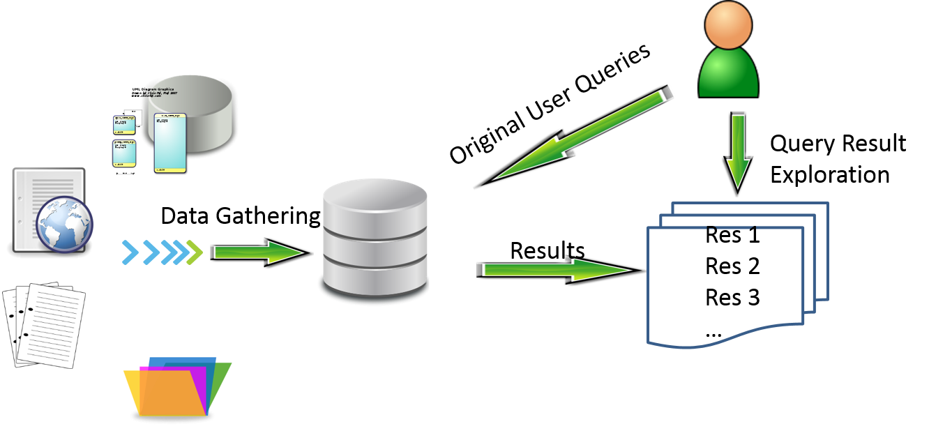
Figure 1: User asks original query and gets results. Now the user explores these results.

For query result exploration, the user selects one or more interesting rows from the results obtained for the original user query, and asks questions such as: why are these rows in the result. The system responds by showing the rows in the tables that combined to produce those results the user is interested in. Different provenance semantics as described in [7, 13] can be used for query result exploration. In this paper, we use the which-provenance semantics (also referred to as lineage) as in [9] and richer semantics is not needed. See Section 6 for a discussion of different provenance semantics.

Table 1: Running Example: Tables (simplified) from TPC-H schema and sample data

$\bf Customers$ $\underline{c\_key}$ $c\_name$ $c\_address$ c1 n1 a1

$\bf Orders$ $\underline{o\_key}$ $c\_key$ $o\_date$ o1 c1 d1 o2 c1 d2

$\bf Lineitem$ $\underline{o\_key}$ $\underline{linenum}$ $qty$ o1 l1 200 o1 l2 150 o2 l1 100 o2 l2 160

Example 1

Consider three tables from TPC-H [1] simplified and with sample data as shown in Table 1. Consider $Q18$ from TPC-H modified as in [15] and simplified for our example. See that the query is defined in [15] in two steps: first a view $Q18\_tmp$ is defined, which is then used to define the original query as view $R$. The results of these two views are also shown.

(find total quantity for each order) SQL: CREATE VIEW $Q18\_tmp$ AS     SELECT $o\_key,sum(qty)$ as $t\_sum\_qty$     FROM $\bf Lineitem$     GROUP BY $o\_key$

$Q18\_tmp$             $o\_key$ $t\_sum\_qty$ o1 350 o2 260

(for each order where total quantity is greater than 300, return the customer and order information, as well as the total quantity) SQL: CREATE VIEW $R$ AS    SELECT $c\_name,c\_key,o\_key,o\_date$,            $sum(qty)$ as $tot\_qty$    FROM $\bf Customers$ NATURAL JOIN $\bf Orders$            NATURAL JOIN $\bf Lineitem$            NATURAL JOIN $Q18\_tmp$    WHERE $t\_sum\_qty>300$    GROUP BY $c\_name$, $c\_key$, $o\_key$, $o\_date$

$R$ $c\_name$ $c\_key$ $o\_key$ $o\_date$ $tot\_qty$ n1 c1 o1 d1 350

$\square$

For this simplified example, there is one row in the result $R$. Suppose the user picks that row and wants to explore that row further. Suppose the user wants to find out what row(s) in the table $\bf Customers$ produced that row. We use $\bf R^{\prime}$ to denote the table consisting of the rows picked by the user for query result exploration. We refer to the row(s) in the $\bf Customers$ table that produced the row(s) in $\bf R^{\prime}$ as the provenance of $\bf R^{\prime}$ for the $\bf Customers$ table, and denote it as $PCustomers$. In [9], the authors come up with a query for determining this provenance shown below. Note that we sometimes use SQL syntax that is not valid, but intuitive and easier.

SELECT $\bf Customers$.* FROM $\bf R^{\prime}$ NATURAL JOIN $\bf Customers$    NATURAL JOIN $\bf Orders$ NATURAL JOIN    $\bf Lineitem$ NATURAL JOIN $Q18\_tmp$ WHERE $t\_sum\_qty>300$

$PCustomers$ $c\_key$ $c\_name$ $c\_address$ c1 n1 a1

However, if we observe closely, we can note the following. Given that the row in $\bf R^{\prime}$ appeared in the result of the original query with the value for $c\_key$ column as $c1$, and given that the key for $\bf Customers$ is $c\_key$, the row from $\bf Customers$ table that produced that row in $R$ must have $c\_key=c1$. Therefore the provenance retrieval query can be simplified as shown below. In this paper (Section 3), we study such optimization of provenance retrieval queries formally.

SELECT $\bf Customers$.* FROM $\bf R^{\prime}$ NATURAL JOIN $\bf Customers$

As another example, consider the provenance of $\bf R^{\prime}$ in the inner $\bf LineItem$ table (used for defining $Q18\_tmp$). This is computed in two steps. First we need to compute $PQ18\_tmp$. Below, we show the $PQ18\_tmp$ query as in [9], and then our optimized $PQ18\_tmp$ query (using the same reasoning as for $PCustomers$).

CREATE VIEW $PQ18\_tmp$ AS SELECT $Q18\_tmp$.* FROM $\bf R^{\prime}$ NATURAL JOIN $\bf Customers$    NATURAL JOIN $\bf Orders$ NATURAL JOIN    $\bf Lineitem$ NATURAL JOIN $Q18\_tmp$ WHERE $t\_sum\_qty>300$

$PQ18\_tmp$ $o\_key$ $t\_sum\_qty$ o1 350

CREATE VIEW $PQ18\_tmp$ AS

SELECT $Q18\_tmp$.* FROM $\bf R^{\prime}$ NATURAL JOIN $Q18\_tmp$

Now, the provenance of $\bf R^{\prime}$ in the inner $\bf LineItem$ table can be computed using the following provenance retrieval query.

SELECT LineItem.* FROM $\bf LineItem$ NATURAL JOIN $PQ18\_tmp$

$PLineitem$ $o\_key$ $linenum$ $qty$ o1 l1 200 o1 l2 150

It is possible to further improve the performance of the above provenance retrieval query if we materialize some additional data. Let us materialize the rows in $R$, along with the corresponding key value(s) from the inner $\bf LineItem$ table for each row in $R$. We denote this result table augmented with additional keys and materialized as $\bf RK$. This will be done as follows.

CREATE VIEW $Q18\_tmpK$ AS SELECT $Q18\_tmp$.*,    $\bf LineItem$$.linenum$ AS linenum2 FROM $Q18\_tmp$ NATURAL JOIN $\bf LineItem$

$Q18\_tmpK$ $o\_key$ $t\_sum\_qty$ $linenum2$ o1 350 l1 o1 350 l2 o2 260 l1 o2 260 l2

CREATE TABLE $\bf RK$ AS SELECT $R$.*, linenum2 FROM $R$ NATURAL JOIN    $Q18\_tmpK$

$\bf RK$ $c\_name$ $c\_key$ $o\_key$ $o\_date$ $tot\_qty$ $linenum2$ n1 c1 o1 d1 350 l1 n1 c1 o1 d1 350 l2

For this example, only the $linenum$ column needs to be added to the columns in $R$ as part of this materialization, because $o\_key$ is already present in $R$ (renamed as $linenum2$ to prevent incorrect natural joins). Now the provenance retrieval query for the inner $\bf LineItem$ table can be defined as follows.

CREATE VIEW $RK^{\prime}$ AS SELECT * FROM $\bf R^{\prime}$ NATURAL JOIN    $\bf RK$

$RK^{\prime}$ $c\_name$ $c\_key$ $o\_key$ $o\_date$ $tot\_qty$ $linenum2$ n1 c1 o1 d1 350 l1 n1 c1 o1 d1 350 l2

SELECT $\bf LineItem$.* FROM $RK^{\prime}$ NATURAL JOIN $\bf LineItem$

See that the provenance retrieval query for the $\bf LineItem$ table in the inner block is now a join of 3 tables: $\bf R^{\prime}$, $\bf RK$ and $\bf LineItem$. Without materialization, the provenance retrieval query involved three joins also: $\bf R^{\prime}$, $Q18\_tmp$ and $\bf LineItem$; however, $Q18\_tmp$ was a view. Our experimental studies confirm the huge performance benefit from this materialization.

Our contributions in this paper include the following:

• We investigate constraints implied in our query result exploration scenario (Section 2.3).

• We investigate optimization of provenance retrieval queries using the constraints. We present our results as a Theorem and we develop an Algorithm based on our theorem (Section 3).

• We investigate materialization of select additional data, and investigate novel hybrid approaches for computing provenance that utilize the constraints and the materialized data (Section 4).

• We perform a detailed performance evaluation comparing our approaches and existing approaches using TPC-H benchmark [1] and report the results (Section 5).

2 Preliminaries

We use the following notations in this paper: a base table is in bold as $\bf T_{i}$, a materialized view is also in bold as $\bf V_{i}$, a virtual view is in italics as $V_{i}$. The set of attributes of table $\bf T_{i}$/materialized view $\bf V_{i}$/virtual view $V_{i}$ is $A_{T_{i}}$/$A_{V_{i}}$/$A_{V_{i}}$; the key for table $\bf T_{i}$ is $K_{i}$. When the distinction between base table or virtual/materialized view is not important, we use $X_{i}$ to denote the table/view; attributes of $X_{i}$ are denoted $A_{X_{i}}$; the key (if defined) is denoted as $K_{i}$.

2.1 Query Language

For our work, we consider SQL queries restricted to ASPJ queries and use set semantics. We do not consider set operators, including union and negation, or outer joins. We believe that extension to bag semantics should be fairly straightforward. However, the optimizations that we consider in this paper are not immediately applicable to unions and outer joins. Extensions to bag semantics, and these additional operators will be investigated in future work. For convenience, we use a Datalog syntax (intuitively extended with group by similar to relational algebra) for representing queries. We consider two types of rules (referred to as SPJ Rule and ASPJ Rule that correspond to SPJ and ASPJ view definitions in [9]) that can appear in the original query as shown in Table 2. A query can consist of one or more rules. Every rule must be safe [20]. Note that Souffle extends datalog with group by. In Souffle, our ASPJ rule will be written as two rules: an SPJ rule and a second rule with the group by. We chose our extension of Datalog (that mimics relational algebra) in this paper for convenience.

Table 2: The two types of rules that can appear in original queries and their Datalog representation. For the ASPJ rule, $GL$ refers to the list of group by columns and $AL$ refers to the list of aggregations.

SPJ Rule:	$R(A_{R})$ :$-$$X_{1}(A_{X_{1}}),X_{2}(A_{X_{2}}),\ldots,X_{n}(A_{X_{n}}).$
ASPJ Rule:	$R(GL,AL)$ :$-$$X_{1}(A_{X_{1}}),X_{2}(A_{X_{2}}),\ldots,X_{n}(A_{X_{n}}).$

Example 2

Consider query $Q18$ from TPC-H (simplified) shown in Example 1 written in Datalog. See that the two rules in $Q18$ are ASPJ rules, where the second ASPJ rule uses the $Q18\_temp$ view defined in the first ASPJ rule. The second rule can be rewritten as an SPJ rule; however, we kept it as an ASPJ rule as the ASPJ rule reflects the TPC-H query faithfully as is also provided in [15].

$Q18\_tmp(o\_key,sum(qty)$ as $t\_sum\_qty)$ :$-$$\bf Lineitem$.

$R$($c\_name$, $c\_key$, $o\_key$, $o\_date$, $sum(qty)$ as $tot\_qty$) :$-$$\bf Customers$, $\bf Orders$,

$\bf Lineitem$, $Q18\_tmp$, $t\_sum\_qty>300.$

$\square$

2.2 Provenance Definition

As said before, we use the which-provenance definition of [9]. In this section, we provide a simple algorithmic definition for provenance based on our rules.

The two types of rules in our program are both of the form: $R(A_{R})$ :$-$$RHS$. We will use $A_{RHS}$ to indicate the union of all the attributes in the relations in $RHS$. For any rule, $R(A_{R})$ :$-$$RHS$, the provenance for $\bf R^{\prime}$ $\subseteq R$ in a table/view $X_{i}(A_{X_{i}})\in RHS$ (that is, the rows in $X_{i}$ that contribute to the results $\bf R^{\prime}$) is given by the program shown in Table 3. See that $PView$ corresponds to the relational representation of why-provenance in [11].

Table 3: Algorithmic Definition of Provenance

Algorithmic definition of provenance for rule: $R(A_{R})$ :$-$$RHS$. The rows in table/view $X_{i}(A_{X_{i}})\in RHS$ that contribute to $\bf R^{\prime}$ $\subseteq R$ are represented as $PX_{i}$.

$PView(A_{R}\cup A_{RHS})$ :$-$$R(A_{R}),RHS.$

$PX_{i}(A_{X_{i}})$ :$-$$PView,$ $\bf R^{\prime}$$(A_{R}).$

Example 3

These examples are based on the schema and sample data in Table 1, and the $Q18\_tmp$ and $R$ views in Example 2.

Consider the definition of view $Q18\_tmp$ in Example 2; rows in the view $Q18\_tmp=\{(o1,350),(o2,260)\}$. Let rows selected to determine provenance $Q18\_tmp^{\prime}=\{(o2,260)\}$.

First $PView$ ($o\_key$,$t\_sum\_qty$, $linenum$, $qty$) is calculated as in Table 3. Here, $PView$ has four rows: { (o1, 350, l1, 200), (o1, 350, l2, 150), (o2, 260, l1, 100), (o2, 260, l2, 160)}

Now $PLineItem$ is calculated (according to Table 3) as:

$PLineItem(o\_key,linenum,qty)$ :$-$$PView,Q18\_tmp^{\prime}.$

The resulting rows for $PLineItem$ = { (o2, l1, 100), (o2, l2, 160)}

$\square$

2.3 Dependencies

We will now examine some constraints for our query result exploration scenario that help optimize provenance retrieval queries. As in Section 2.2, the original query is of the form $R(A_{R})$ :$-$$RHS$; and $A_{RHS}$ indicates the union of all the attributes in the relations in $RHS$. Furthermore, $\bf R^{\prime}$ $\subseteq R$. We express the constraints as tuple generating dependencies below. While these dependencies are quite straightforward, they lead to significant optimization of provenance computation as we will see in later sections.

Dependency 1

$\forall A_{R},$ $\bf R^{\prime}$$(A_{R})\rightarrow R(A_{R})$

Dependency 1 is obvious as the rows for which we compute the provenance, $\bf R^{\prime}$ is such that $\bf R^{\prime}$ $\subseteq R$. For the remaining dependencies, consider $RHS$ as the join of the tables $X_{1}(A_{X_{1}}),X_{2}(A_{X_{2}}),\ldots,X_{n}(A_{X_{n}})$, as shown in Table 2.

Dependency 2

$\forall A_{R},\ R(A_{R})\rightarrow\exists(A_{RHS}-A_{R}),$ $X_{1}(A_{X_{1}}),$ $X_{2}(A_{X_{2}}),\ldots,X_{n}(A_{X_{n}})$

Dependency 2 applies to both the rule types shown in Table 2. As any row in $R$ is produced by the join of $X_{1}(A_{X_{1}}),X_{2}(A_{X_{2}}),\ldots,X_{n}(A_{X_{n}})$, Dependency 2 is also obvious. From Dependencies 1 and 2, we can infer the following dependency.

Dependency 3

$\forall A_{R},$ $\bf R^{\prime}$ $(A_{R})\rightarrow\exists(A_{RHS}-A_{R}),$ $X_{1}(A_{X_{1}}),$ $X_{2}(A_{X_{2}}),\ldots,X_{n}(A_{X_{n}})$

3 Optimizing Provenance Queries without materialization

Consider the query for computing provenance given in Table 3 after composition: $PX_{i}(A_{X_{i}})$ :$-$$R(A_{R}),RHS,$ $\bf R^{\prime}$$(A_{R}).$ Using Dependency 1, one of the joins in the query for computing provenance can immediately be removed. The program for computing provenance of $\bf R^{\prime}$ $\subseteq R$ in table/view $X_{i}$ is given by the following program. See that $X_{i}$ can be a base table or a view.

Program 1

$PX_{i}(A_{i})$ :$-$$\bf R^{\prime}$$(A_{R}),RHS$.

Program 1 is used by [9] for computing provenance. However, we will optimize Program 1 further using the dependencies in Section 2.3. Let $P_{1}$ below indicate the query in Program 1. Consider another query $P_{2}$ (which has potentially fewer joins than $P_{1}$). Theorem 3.1 states when $P_{1}$ is equivalent to $P_{2}$. The proof uses the dependencies in Section 2.3 and is omitted.

$P_{1}:PX_{i}(A_{X_{i}})$ :$-$$\bf R^{\prime}$$(A_{R}),$ $X_{1}(A_{X_{1}}),X_{2}(A_{X_{2}}),\ldots,X_{n}(A_{X_{n}})$.
$P_{2}:PX_{i}(A_{X_{i}})$ :$-$$\bf R^{\prime}$, $X_{j_{1}}(A_{X_{j_{1}}}),X_{j_{2}}(A_{X_{j_{2}}}),\ldots,X_{j_{q}}(A_{X_{j_{q}}})$.,
                                 where $\{j_{1},j_{2},\ldots,j_{q}\}$ $\subseteq$ $\{1,2,\ldots,n\}$

Notation. For convenience, we introduce two notations below. $A_{RHS}^{\prime}=A_{X_{j_{1}}}\cup A_{X_{j_{2}}}\cup\ldots\cup A_{X_{j_{q}}}$. Consider the tables that are present in the RHS of $P_{1}$, but not in the RHS of $P_{2}$. $A_{RHS}^{\prime\prime}$ denotes all the attributes in these tables.

Theorem 3.1

Queries $P_{1}$ and $P_{2}$ are equivalent, if for every column $C\in A_{RHS}^{\prime}$, at least one of the following is true:

• $A_{R}\rightarrow C$ (that is, $A_{R}$ functionally determines $C$)

• $C\notin A_{RHS}^{\prime\prime}$

Based on Theorem 3.1, we can infer the following corollaries. Corollary 1 says that if all the columns of $X_{i}$ are present in the result, no join is needed to compute the provenance of $X_{i}$. Corollary 2 says that if a key of $X_{i}$ is present in the result, then the provenance of $X_{i}$ can be computed by joining $\bf R^{\prime}$ and $X_{i}$.

Corollary 1

If $A_{X_{i}}\subseteq A_{R}$, then $PX_{i}(A_{X_{i}})$ :$-$$\bf R^{\prime}$$(AR).$

Corollary 2

If $K_{i}\subseteq A_{R}$, then $PX_{i}(A_{X_{i}})$ :$-$$\bf R^{\prime}$$(AR)$, $X_{i}(A_{X_{i}}).$

3.1 Provenence Query Optimization Algorithm

In this section, we will come with an algorithm based on Theorem 3.1 that starts with the original provenance retrieval query and comes up with a new optimized provenance retrieval query with fewer joins. Suppose the original user query is: $R(A_{R})$ :$-$$X_{1}(A_{X_{1}})$, $X_{2}(A_{X_{2}})$, $\ldots$, $X_{n}(A_{X_{n}})$. The user wants to determine the rows in $X_{i}$ that contributed to the results $\bf R^{\prime}$$(A_{R})\subseteq R(A_{R})$. Note that $X_{i}$ can either be a base table or a view.

Algorithm 1 Efficient Provenance Retrieval Query

1:start with $CurRHS=$ $\bf R^{\prime}$$(A_{R})$

2:if $A_{X_{i}}\subseteq A_{R}$ then return $CurRHS$

3:add $X_{i}$ to $CurRHS$

4:let $CurRHSTables=X_{i}$; $A_{RHS}^{\prime}=\bigcup A_{X_{j}}$, where $X_{j}\in CurRHSTables$

5:let $RemTables$ = $\{X_{1},X_{2},\ldots,X_{n}\}$ -$X_{i}$; $A_{RHS}^{\prime\prime}=\bigcup A_{X_{j}}$, where $X_{j}\in RemTables$

6:while there is a column $C\in A_{RHS}^{\prime}\ \cap\ A_{RHS}^{\prime\prime}$, and there is no functional dependency $A_{R}\rightarrow C$ do

7:     Add all tables in $RemTables$ that have the column $C$ to $CurRHS$, and to $CurRHSTables$. Adjust $A_{RHS}^{\prime}$, $RemTables$, $A_{RHS}^{\prime\prime}$ appropriately.

8:return $CurRHS$

Illustration of Algorithm 1

Consider the SPJA rule for $R$ for Q18 in TPC-H from Example 2.

$R(c\_name,c\_key,o\_key,o\_date,sum(qty)$ as $total\_qty)$ :$-$
     $\bf Customers$, $\bf Orders$, $\bf Lineitem$, $Q18\_tmp,t\_sum\_qty>300.$

Algorithm 1 produces the provenance retrieval query for $\bf Customers$ as follows. After line 3, $CurRHS=$ $\bf R^{\prime}$, $\bf Customers$. At line 6, $A_{RHS}^{\prime}\cap A_{RHS}^{\prime\prime}$ = $\{c\_key\}$. As $c\_key\in A_{R}$, and $A_{R}\rightarrow c\_key$, no more tables are added to $CurRHS$. Thus, the final provenance retrieval query is: $PCustomers$ :$-$$\bf R^{\prime}$, $\bf Customers$.

4 Optimizing Provenance Queries with materialization

In Section 3, we studied optimizing the provenance retrieval queries for the lazy approach, where no additional data is materialized. Eager and hybrid approaches materialize additional data. An eager approach could be to materialize $PView$ (defined in Table 3). However, $PView$ could be a very large table with several columns and rows of data. In this section, we investigate novel hybrid approaches that materialize much less additional data, and perform comparable to (and often times, even better than) the eager approach that materializes $PView$. The constraints identified in Section 2.3 are still applicable, and are used to decrease the joins in the provenance retrieval queries.

A user query can have multiple rules that form multiple steps (for instance, Q18 in TPC-H has two steps). While our results apply for queries with any number of steps, for simplicity of illustration, we consider only queries with two steps (the results extend in a straightforward manner to any number of steps). A query with two steps is shown in Figure 2. The Datalog program corresponding to Figure 2 is shown in Program 2. $R$ is the result of the query. $R$ is defined using the base tables $\bf T_{1}$, $\bf T_{2}$, $\ldots$, $\bf T_{n}$, and the views $V_{1}$, $V_{2}$, $\ldots$, $V_{m}$. Remember that from Section 2, $\bf T_{1}$ has attributes $A_{T_{1}}$ and key attributes $K_{1}$; $\bf T_{1{n_{1}}}$ has attributes $A_{T_{1{n_{1}}}}$ and key attributes $K_{1{n_{1}}}$; $V_{1}$ has attributes $A_{V_{1}}$.

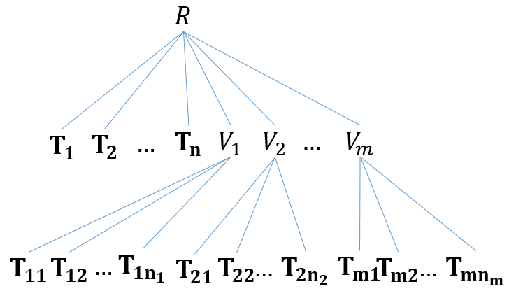
Figure 2: Query with two steps

Program 2

$V_{i}(A_{V_{i}})$ :$-$$\bf T_{i1}$, $\bf T_{i2}$, …, $\bf T_{in_{i}}$.        $\forall$ $i\in 1,2,...,m$

$R(A_{R})$ :$-$$\bf T_{1}$, $\bf T_{2}$, …, $\bf T_{n}$, $V_{1},V_{2},\ldots,V_{m}$.

Given a query $R$ as in Program 2, we materialize a view $\bf RK$ with columns $A_{RK}$. $A_{RK}$ consists of the columns $A_{R}$ in $R$ and the keys of zero or more of the base tables used in $R$ (how $A_{RK}$ is determined is discussed later). $\bf RK$ is defined using $R$, the base tables that define $R$ and the $VK_{i}$ views corresponding to each of the $V_{i}$ that define $R$. See Program 3. $VK_{i}$ is a virtual view defined using $V_{i}$ and the tables that define $V_{i}$. If no keys are added to $V_{i}$ to form $VK_{i}$ (i.e., $A_{VK_{i}}$ = $A_{V_{i}}$), then $VK_{i}$ can be optimized to be just $V_{i}$. Algorithm 1 can be used to optimize $VK_{i}$ and $\bf RK$ as well; details are omitted.

Program 3

$V_{i}(A_{V_{i}})$ :$-$$\bf T_{i1}$, $\bf T_{i2}$, …, $\bf T_{in_{i}}$.        $\forall$ $i\in 1,2,...,m$

$R(A_{R})$ :$-$$\bf T_{1}$, $\bf T_{2}$, …, $\bf T_{n}$, $V_{1},V_{2},\ldots,V_{m}$.

$VK_{i}(A_{VK_{i}})$ :$-$$V_{i}$, $\bf T_{i1}$, $\bf T_{i2}$, …, $\bf T_{in_{i}}$.  $\forall$ $i\in 1,2,...,m$

$\bf RK$$(A_{RK})$ :$-$$R$, $\bf T_{1}$, $\bf T_{2}$, …, $\bf T_{n}$, $VK_{1}$, $VK_{2}$, $\ldots$, $VK_{m}$.

$OQ(A_{R})$ :$-$$\bf RK$.

The original user query results (computed as $R$ in Program 2) are computed by $OQ$ in Program 3. This is because we assume that $\bf RK$ is materialized during the original user query execution and we expect that computing $OQ$ from $\bf RK$ will be faster than computing the results of $R$.

For query result exploration, suppose that the user selects $\bf R^{\prime}$ $\subseteq R$ and wants to find the provenance of $\bf R^{\prime}$ in the table $\bf T_{i}$. We will assume that $\bf T_{i}$ is a base table that defines $V_{j}$. For this, we first define $RK^{\prime}\subseteq$ $\bf RK$ as shown below.

$RK^{\prime}$ :$-$$\bf R^{\prime}$,$\bf RK$.

$RK^{\prime}$ denotes the rows in $\bf RK$ corresponding to the rows in $\bf R^{\prime}$. Now to compute the provenance of $\bf R^{\prime}$ in the table $\bf T_{i}$, we compute the provenance of $RK^{\prime}$ in the table $\bf T_{i}$. There are two cases:

Program 4

Case 1:	$K_{i}\subseteq A_{RK}$:	$PT_{i}$ :$-$$RK^{\prime}$, $\bf T_{i}$.
Case 2:	$K_{i}\nsubseteq A_{RK}$:	$PT_{i}$ :$-$$PV_{j},V_{jRHS}$.
($V_{jRHS}$ is the RHS of the rule that defines $V_{j}$.)

Case 1 is similar to Corollary 2 except that $R$ may not be defined using $\bf T_{i}$ directly. For Case 2, $V_{j}$ is defined using $\bf T_{i}$ directly. $PV_{j}$ is the provenance of $RK^{\prime}$ in the view $V_{j}$, computed recursively using Program 4. Given $PV_{j}$, the rule for computing the provenance of $PV_{j}$ in the table $\bf T_{i}$ is given by Program 1. Both the rules in Program 4 can be optimized using Algorithm 1.

Example 4

Consider $Q18$ from Example 2. There are 4 base tables used in $Q18$ – $\bf Customers$, $\bf Orders$, $\bf Lineitem1$ and $\bf Lineitem2$. We distinguish the two $\bf Lineitem$ tables; $\bf Lineitem2$ denotes the table used in $Q18\_tmp$ definition.

The materialized $\bf RK$ view contains the columns in $R$ and additionally the key for $\bf Lineitem2$ table. The key for the $\bf Lineitem2$ table is $(o\_key,linenum)$; however $o\_key$ is already present in $R$. Therefore only the $linenum$ column from $\bf Lineitem2$ is added in $A_{RK}$. The revised program (as in Program 3) that materializes $\bf RK$ and computes $OQ$ is shown below. Note that optimizations as in Algorithm 1 are applicable (for example, definition of $\bf RK$); details are omitted.

$Q18\_tmp(o\_key,sum(qty)$ as $t\_sum\_qty)$ :$-$$\bf Lineitem$.

$R(c\_name,c\_key,o\_key,o\_date,o\_totalprice,sum(qty)$ as $total\_qty)$

:$-$$\bf Customers$, $\bf Orders$, $\bf Lineitem$, $Q18\_tmp,t\_sum\_qty>300.$

$Q18\_tmpK(o\_key,linenum$ as $linenum2,t\_sum\_qty)$ :$-$$Q18\_tmp$, $\bf Lineitem$.

$\bf RK$$(c\_name$, $c\_key$, $o\_key$, $o\_date$, $o\_totalprice$, $linenum2$, $total\_qty)$

:$-$$R,Q18\_tmpK.$

$OQ(c\_name,c\_key,o\_key,o\_date,o\_totalprice,total\_qty)$ :$-$$\bf RK$.

Let $\bf R^{\prime}$ denote the selected rows in $R$ whose provenance we want to explore. To compute their provenance, we first need to determine which rows in $\bf RK$ correspond to the rows in $\bf R^{\prime}$. This is done as:

$RK^{\prime}(A_{RK})$ :$-$$\bf R^{\prime}$, $\bf RK$.

Now, we need to compute the provenance of the rows in $RK^{\prime}$ from the different tables, which is computed as follows. See that all the rules have been optimized using Algorithm 1, and involve a join of $RK^{\prime}$ and one base table.

$PCustomers(c\_key,c\_name,c\_address)$ :$-$$RK^{\prime}$, $\bf Customers$.

$POrders(o\_key,c\_key,o\_date,o\_totalprice)$ :$-$$RK^{\prime}$, $\bf Orders$.

$PLineitem1(o\_key,linenum,qty)$ :$-$$RK^{\prime}$, $\bf Lineitem$.

$PLineitem2(o\_key,linenum,qty)$ :$-$$RK^{\prime}$ $(c\_name$, $c\_key$, $o\_key$,

$o\_date$, $o\_totalprice$, $linenum2$ as $linenum$, $total\_qty)$, $\bf Lineitem$.

$\square$

4.1 Determining the keys to be added to the materialized view

When we materialize $\bf RK$, computing the results of the original user query is expected to take longer because we consider that materialization of $\bf RK$ is done during original query execution, and because $\bf RK$ is expected to be larger than the size of $R$: the number of rows (and the number of columns) in $\bf RK$ will not be fewer than the number of rows (and the number of columns) in $R$. However, materialization typically benefits result exploration because the number of joins to compute the provenance for some of the base tables is expected to be smaller (although it is possible that the size of $\bf RK$ might be large and this may slow down the provenance computation).

For the materialized view $\bf RK$, we consider adding keys of the different base tables and compute the cost .vs. benefit. The ratio of the estimated number of rows of $\bf RK$ and the estimated number of rows in $R$ forms the cost. The ratio of the number of joins across all provenance computations of base tables with and without materialization give the benefit. We use a simple cost model that combines the cost and the benefit to determine the set of keys to be added to $\bf RK$. For the example query $Q18$, the provenance retrieval queries for $\bf Customers$, $\bf Orders$ and $\bf Lineitem$ tables in the outer block already involve only one join. Therefore no keys need to be added to improve the performance of these three provenance retrieval queries. However, we can improve the performance of the provenance retrieval query for the $\bf Lineitem$ table in the inner block by adding the keys for the inner $\bf Lineitem$ table to $\bf RK$ as shown in Example 4.

For $\bf RK$, we currently consider adding the key for every base table as part of the cost-benefit analysis. In other words, the number of different hybrid options we consider is exponential in the number of tables in the original user query. For each option, the cost .vs. benefit is estimated and one of the options is selected. As part of future work, we are investigating effective ways of searching this space. Other factors may be included in our cost model to determine which keys to be added to $\bf RK$, including the workload of provenance queries.

5 Evaluation

For our evaluation, we used the TPC-H [1] benchmark. We generated data at 1GB scale. Our experiments were conducted on a PostgreSQL 10 database server running on Windows 7 Enterprise operating system. The hardware included a 4-core Intel Xeon 2.5 GHz Processor with 128 GB of RAM. For our queries, we again used the TPC-H benchmark. The queries provided in the benchmark were considered the original user queries. Actually, we considered the version of the TPC-H queries provided by [15], which specifies values for the parameters for the TPC-H benchmark and also rewrites nested queries. For the result exploration part, we considered that the user would pick one row in the result of the original query (our solutions apply even if multiple rows were picked) and ask for the rows in the base tables that produce that resulting row.

We compare the following approaches:

• The approach in [9] that we refer to as: W (lazy approach). No additional data is materialized; the materialization studied in [8] is not considered.

• The approach in [11] that we refer to as: G. Here we assume that the relational representation of provenance is materialized while computing the original user query (eager approach). Provenance computation is then translated into mere look-ups in this materialized data.

• Algorithm 1 without materialization that we refer to as: O1 (lazy approach).

• Our approach with materialization from Section 4 that we refer to as: O2 (hybrid approach).

5.1 Usefulness of our optimization rules

Algorithm 1 results in queries with much fewer joins. We tested the provenance retrieval queries for $Q18$ from TPC-H as given in [15] (for our experiments, the schema and the queries were not simplified as in our running example). The times observed are listed in Table 4. See that the provenance retrieval queries generated by Algorithm 1 (O1) run much faster than the ones used in [9] (W).

Table 4: O1 compared to W for $Q18$ in [15]. All times are reported in milliseconds.

	$PCustomers$	$POrders$	$PLineItem$
O1	0.07	0.06	0.30
W	1522.44	1533.88	1532.74

We considered all the TPC-H queries as given in [15] except for the ones with outer joins (as we do not consider outer joins in this paper). Of the 22 TPC-H queries, the queries with outer joins are Q13, Q21, Q22, and these were not considered. $Q19$ has $or$ in its predicate, which can be rewritten as a union. However, we considered the $or$ predicate as a single predicate without breaking it into a union of multiple rules. For 7 out of these 19 queries, O1 results in provenance retrieval queries with fewer joins than the ones in W. They were Q2, Q3, Q7, Q10, Q11, Q15 and Q18. In other words, Algorithm 1 was useful for around 36.84% of the TPC-H queries.

5.2 Usefulness of materialization

For $Q18$ [15], we compared the time to compute the original query results (OQ) and the time to compute the provenance of the four tables for the four approaches: O1, W, G and O2. The materialized view $\bf RK$ in O2 included the key for the $\bf LineItem$ table in the inner block. The results are shown in Table 5.

Table 5: Performance Benefits of materialization proposed in Section 4 for Q18 in [15]. All times are reported in milliseconds.

	O1	W	G	O2
OQ	5095.67	5095.67	5735446.19	13794.26
PCustomers	0.07	1522.44	3.86	0.96
POrders	0.06	1533.88	3.73	0.43
PLineItem1	0.30	1532.74	5.77	0.59
PLineItem2	1641.52	1535.22	6.16	0.43

There are several points worth observing in Table 5. We typically expect O2 to outperform G in computing the results of the original user query. This is because G maintains all the columns of every base table in the materialized view, whereas O2 maintains only some key columns in the materialized view - in this case, the materialized view consists of the columns in $R$ and only one addition column $linenum2$. The performance impact of this is significant as G takes about 420 times the time taken by O2 to compute the results of the original user query. Actually the time taken by G is about 5700 seconds, which is likely to be unacceptable. On the other hand, O2 takes about 2.7 times the time taken by O1 for computing the results of the original user query. Drilling down further, we found that computing the results from the materialized view $\bf RK$ took about 0.39 milliseconds for O2 and about 3.07 milliseconds for G (Table 6(b)).

Table 6: (a) Comparing the size of the tables: R (result of the original user query), RK_G (materialized view RK used by G) and RK_O2 (materialized view RK used by O2). (b) Comparing time for computing materialized view RK and time for computing original query results from RK for Q18 [15]. All times are reported in milliseconds.

R RK_G RK_O2 # Columns 6 51 7 # Rows 57 2793 399	G O2 Computing RK 5735443.12 13793.88 Computing OQ from RK 3.07 0.39
(a)	(b)

We expect G to outperform O2 in computing the provenance. This is because the provenance retrieval in G requires a join of $\bf R^{\prime}$ with $\bf RK$. O2 requires a join of 3 tables (if the key is included in $\bf RK$). For Q18, the provenance retrieval query for $LineItem2$ requires a join of $\bf R^{\prime}$ with $\bf RK$ to produce $RK^{\prime}$, which is then joined with $\bf LineItem$ table. However the larger size of $\bf RK$ in G (Table 6(a)) results in O2 outperforming G for provenance retrieval (Table 5).

In practice, O2 will never perform worse than O1 for provenance retrieval. This is because for any table, the provenance retrieval query for O1 (that does not use $RK^{\prime}$, but instead uses $\bf R^{\prime}$) may be used instead of the provenance retrieval query for O2 (that uses $RK^{\prime}$ as in Program 4) if we expect the performance of the provenance retrieval query for O1 to be better. However, we have not considered this optimization in this paper.

Other things to note are that computing the results of the original query for $O1$ and $W$ is done exactly the same way. Moreover, for $Q18$, O1 outperforms all approaches even in provenance retrieval except for $PLineItem2$. This is because Algorithm 1 is able to optimize the provenance retrieval queries significantly for $PCustomers$, $POrders$, $PLineItem1$. However, for $PLineItem2$, the provenance retrieval required computing $PQ18\_tmp$ and then using it to compute $PLineItem2$, which needed more joins. Usually, we expect every provenance retrieval query from O1 to outperform W, but in this case W did outperform O1 for $PLineItem2$ (by a small amount); we believe the reason for this is the extra joins in W ended up being helpful for performance (which is not typical).

We report on the 19 TPC-H queries without outer joins in Table 7. In this table, OQ refers to the time taken for computing the results of the original user query, AP (average provenance) refers to the time taken to compute the provenance averaged over all the base tables used in the query, and MP (minimum provenance) refers to the minimum time to compute provenance over all the base tables used in the query. For W, we typically expect AP and MP to be almost the same (unless for nested queries); this is because in W, every provenance retrieval query (for non-nested original user queries) performs the same joins. Similarly for G, we typically expect AP and MP to be almost the same (because every provenance computation is just a look-up in the materialized data), except for the difference in the size of the results. For O1 and O2, MP might be significantly smaller than AP because some provenance computation might have been optimized extensively (example: Q2, Q10, Q11, Q15, Q18).

Table 7: Summary of experiments. The times are reported in milliseconds to two decimal places accuracy. However, considering the width of the table, if the time is 100 ms or greater, we report in scientific notation with two significant numbers.

	O1			W			G			O2
	OQ	AP	MP	OQ	AP	MP	OQ	AP	MP	OQ	AP	MP
Q1	3.4e3	3.2e3	3.2e3	3.4e3	3.2e3	3.2e3	1.5e5	3.7e4	3.7e4	1.1e5	2.7e4	2.7e4
Q2	55.88	37.41	0.21	55.88	55.59	43.03	1.3e4	1.25	0.98	7.7e3	0.61	0.52
Q3	8.7e2	0.06	0.04	8.7e2	0.09	0.08	2.9e3	45.57	43.11	2.5e3	4.28	3.47
Q4	4.1e3	5.3e3	4.3e3	4.1e3	5.3e3	4.3e3	3.3e4	1.6e2	1.4e2	7.7e3	4.5e2	3.5e2
Q5	6.3e2	6.7e2	6.5e2	6.3e2	6.7e2	6.5e2	2.9e3	13.01	10.71	2.5e3	11.45	4.73
Q6	6.2e2	6.7e2	6.7e2	6.3e2	6.7e2	6.7e2	3.2e3	90.28	90.28	2.9e3	9.0e2	9.0e2
Q7	8.7e2	6.7e2	6.6e2	8.7e2	6.7e2	6.6e2	4.9e3	13.22	11.12	4.5e3	12.26	6.88
Q8	8.3e2	1.7e3	1.6e3	8.3e2	1.7e3	1.6e3	4.1e3	5.05	2.17	3.3e3	7.92	3.74
Q9	3.7e3	2.3e6	2.2e6	3.7e3	2.3e6	2.2e6	2.2e5	1.7e2	1.7e2	1.9e5	7.2e2	1.0e2
Q10	1.5e3	99.69	0.06	1.5e3	1.3e2	1.3e2	9.6e6	1.1e2	1.1e2	3.1e3	1.0e2	30.27
Q11	4.3e2	2.6e2	4.06	4.3e2	6.0e2	3.9e2	1.9e6	8.2e4	7.4e4	1.3e3	3.1e2	0.58
Q12	8.9e2	7.9e2	7.8e2	8.9e2	7.9e2	7.8e2	4.0e3	9.15	8.60	3.9e3	30.00	21.31
Q14	7.7e2	9.8e2	9.2e2	7.7e2	9.8e2	9.2e2	4.3e3	1.8e2	1.7e2	3.3e3	5.8e2	2.8e2
Q15	1.43e3	1.0e3	4.62	1.4e3	2.2e3	1.4e3	2.0e5	6.0e4	3.0e4	1.7e5	9.7e4	5.5e4
Q16	1.2e3	1.3e2	1.1e2	1.2e3	1.3e2	1.1e2	4.9e3	55.37	54.03	2.6e3	2.2e2	2.2e2
Q17	4.2e3	5.9e3	4.3e3	4.2e3	5.9e3	4.3e3	2.2e4	41.79	37.96	2.2e4	4.3e3	4.3e3
Q18	5.1e3	4.1e2	0.06	5.1e3	1.5e3	1.5e3	5.7e6	4.88	3.73	1.4e4	0.60	0.43
Q19	2.4e3	2.4e3	2.4e3	2.4e3	2.4e3	2.4e3	1.3e4	13.35	12.62	1.3e4	86.23	83.44
Q20	2.0e3	2.3e3	1.9e3	2.0e3	2.3e3	1.9e3	6.9e4	0.34	0.28	4.0e3	5.6e2	0.21

We find that except for one single table query Q1, where W performs same as O1, our approaches improve performance for provenance computation, and hence for result exploration. Furthermore, the eager materialization approach (G) could result in prohibitively high times for original result computation.

6 Related Work

Different provenance semantics as described in [7, 13] can be used for query result exploration. Lineage, or which-provenance [9] specifies which rows from the different input tables produced the selected rows in the result. why-provenance [5] provides more detailed explanation than which-provenance and collects the input tuples separately for different derivations of an output tuple. how-provenance [12, 7, 13] provides even more detailed information than why-provenance and specifies how the different input table rows combined to produce the result rows. Trio [3] provides a provenance semantics similar to how-provenance as studied in [7]. Deriving different provenance semantics from other provenance semantics is studied in [7, 13]: how-provenance provides the most general semantics and can be used to compute other provenance semantics [7]. A hierarchy of provenance semirings that shows how to compute different provenance semantics is explained in [13]. Another provenance semantics in literature is where-provenance [5], which only says where the result data is copied from. Provenance of non-answers studies why expected rows are not present in the result and is studied in [16, 6, 14]. Explaining results using properties of the data are studied in [18, 19].

For our work, we choose which-provenance even though it provides less details than why and how provenance because: (a) which-provenance is defined for queries with aggregate and group by operators [13] that we study in this paper, (b) which-provenance is complete [7], in that all the other provenance semantics provide explanations that only include the input table rows selected by which-provenance. As part of our future work, we are investigating computing other provenance semantics starting from which-provenance and the original user query, (c) which-provenance is invariant under equivalent queries (provided tables in self-joins have different and ”consistent” names), thus supporting correlated queries (d) results of which-provenance is a set of tables that can be represented in the relational model without using additional features as needed by how-provenance, or a large number of rows as needed by why-provenance.

When we materialize data for query result exploration, the size of the materialized data can be an issue as identified by [13]. Eager approaches record annotations (materialized data) which are propagated as part of provenance computation [4]. A hybrid approach that uses materialized data for computing provenance in data warehouse scenario as in [9] is studied in [8]. In our work, we materialize the results of some of the intermediate steps (views). While materializing the results of an intermediate step, we augment the result with the keys of some of the base tables used in that step. Note that the non-key columns are not stored, and the keys for all the tables may not need to be stored; instead, we selectively choose the base tables whose keys are stored based on the expected benefit and cost, and based on other factors such as workload.

Other scenarios have been considered. For instance, provenance of non-answers are considered in [6, 14]. In [16], the authors study a unified approach for provenance of answers and non-answers. However, as noted in [13], research on negation in provenance has so far resulted in divergent approaches. Another scenario considered is explaining results using properties of the data [18, 19].

Optimizing queries in the presence of constraints has long been studied in database literature, including chase algorithm for minimizing joins [2]. Join minimization in SQL systems has typically considered key-foreign key joins [10]. Optimization specific to provenance queries is studied in [17]. Here the authors study heuristic and cost based optimization for provenance computation. The constraints we study in this paper are tuple generating dependencies as will occur in scenario of query result exploration; these are more general than key-foreign key constraints. We develop practical polynomial time algorithms for join minimization in the presence of these constraints.

7 Conclusions and Future Work

In this paper, we studied dependencies that are applicable to query result exploration. These dependencies can be used to optimize query performance during query result exploration. For the TPC-H benchmark, we could optimize the performance of 36.84% (7 out of 19) of the queries that we considered. Furthermore, we investigated how additional data can be materialized and then be used for optimizing the performance during query result exploration. Such materialization of data can optimize the performance of query result exploration for almost all the queries.

One of the main avenues worth exploring is extensions to the query language that we considered. The dependencies we considered can be used when the body of a rule is a conjunction of predicates. We did not consider union queries, negation or outer joins. These will be interesting to explore as the dependencies do not extend in a straightforward manner. Another interesting future direction is studying effective ways of navigating the search space of possible materializations. Also, it will be worthwhile investigating how to start from provenance tables and define other provenance semantics (such as how-provenance) in terms of the provenance tables.

References

- [1] TPC-H, a decision support benchmark, available at http://www.tpc.org/tpch/ (2018), http://www.tpc.org/tpch/
- [2] Abiteboul, S., Hull, R., Vianu, V.: Foundations of Databases. Addison-Wesley (1995), http://webdam.inria.fr/Alice/
- [3] Benjelloun, O., Sarma, A.D., Halevy, A.Y., Theobald, M., Widom, J.: Databases with uncertainty and lineage. VLDB J. 17(2), 243–264 (2008). https://doi.org/10.1007/s00778-007-0080-z, https://doi.org/10.1007/s00778-007-0080-z
- [4] Bhagwat, D., Chiticariu, L., Tan, W.C., Vijayvargiya, G.: An annotation management system for relational databases. VLDB J. 14(4), 373–396 (2005). https://doi.org/10.1007/s00778-005-0156-6, https://doi.org/10.1007/s00778-005-0156-6
- [5] Buneman, P., Khanna, S., Tan, W.C.: Why and where: A characterization of data provenance. In: Database Theory - ICDT 2001, 8th International Conference, London, UK, January 4-6, 2001, Proceedings. pp. 316–330 (2001). https://doi.org/10.1007/3-540-44503-X_20, https://doi.org/10.1007/3-540-44503-X_20
- [6] Chapman, A., Jagadish, H.V.: Why not? In: Proceedings of the ACM SIGMOD International Conference on Management of Data, SIGMOD 2009, Providence, Rhode Island, USA, June 29 - July 2, 2009. pp. 523–534 (2009). https://doi.org/10.1145/1559845.1559901, https://doi.org/10.1145/1559845.1559901
- [7] Cheney, J., Chiticariu, L., Tan, W.C.: Provenance in databases: Why, how, and where. Foundations and Trends in Databases 1(4), 379–474 (2009). https://doi.org/10.1561/1900000006, https://doi.org/10.1561/1900000006
- [8] Cui, Y., Widom, J.: Storing auxiliary data for efficient maintenance and lineage tracing of complex views. In: Proceedings of the Second Intl. Workshop on Design and Management of Data Warehouses, DMDW 2000, Stockholm, Sweden, June 5-6, 2000. p. 11 (2000), http://ceur-ws.org/Vol-28/paper11.pdf
- [9] Cui, Y., Widom, J., Wiener, J.L.: Tracing the lineage of view data in a warehousing environment. ACM Trans. Database Syst. 25(2), 179–227 (2000). https://doi.org/10.1145/357775.357777, https://doi.org/10.1145/357775.357777
- [10] Eder, L.: Join elimination: An essential optimizer feature for advanced sql usage. DZone (2017), https://dzone.com/articles/join-elimination-an-essential-optimizer-feature-fo
- [11] Glavic, B., Miller, R.J., Alonso, G.: Using SQL for efficient generation and querying of provenance information. In: Search of Elegance in the Theory and Practice of Computation - Essays Dedicated to Peter Buneman. pp. 291–320 (2013). https://doi.org/10.1007/978-3-642-41660-6_16, https://doi.org/10.1007/978-3-642-41660-6_16
- [12] Green, T.J., Karvounarakis, G., Tannen, V.: Provenance semirings. In: Proceedings of the Twenty-Sixth ACM SIGACT-SIGMOD-SIGART Symposium on Principles of Database Systems, June 11-13, 2007, Beijing, China. pp. 31–40 (2007). https://doi.org/10.1145/1265530.1265535, https://doi.org/10.1145/1265530.1265535
- [13] Green, T.J., Tannen, V.: The semiring framework for database provenance. In: Proceedings of the 36th ACM SIGMOD-SIGACT-SIGAI Symposium on Principles of Database Systems, PODS 2017, Chicago, IL, USA, May 14-19, 2017. pp. 93–99 (2017). https://doi.org/10.1145/3034786.3056125, https://doi.org/10.1145/3034786.3056125
- [14] Huang, J., Chen, T., Doan, A., Naughton, J.F.: On the provenance of non-answers to queries over extracted data. PVLDB 1(1), 736–747 (2008). https://doi.org/10.14778/1453856.1453936, http://www.vldb.org/pvldb/1/1453936.pdf
- [15] Jia, Y.: Running the TPC-H benchmark on Hive (2009), https://issues.apache.org/jira/browse/HIVE-600
- [16] Lee, S., Ludäscher, B., Glavic, B.: PUG: a framework and practical implementation for why and why-not provenance. VLDB J. 28(1), 47–71 (2019). https://doi.org/10.1007/s00778-018-0518-5, https://doi.org/10.1007/s00778-018-0518-5
- [17] Niu, X., Kapoor, R., Glavic, B., Gawlick, D., Liu, Z.H., Krishnaswamy, V., Radhakrishnan, V.: Heuristic and cost-based optimization for diverse provenance tasks. CoRR abs/1804.07156 (2018), http://arxiv.org/abs/1804.07156
- [18] Roy, S., Orr, L., Suciu, D.: Explaining query answers with explanation-ready databases. PVLDB 9(4), 348–359 (2015). https://doi.org/10.14778/2856318.2856329, http://www.vldb.org/pvldb/vol9/p348-roy.pdf
- [19] Wu, E., Madden, S.: Scorpion: Explaining away outliers in aggregate queries. PVLDB 6(8), 553–564 (2013). https://doi.org/10.14778/2536354.2536356, http://www.vldb.org/pvldb/vol6/p553-wu.pdf
- [20] Zaniolo, C., Ceri, S., Faloutsos, C., Snodgrass, R.T., Subrahmanian, V.S., Zicari, R.: Advanced Database Systems. Morgan Kaufmann (1997)