Resonant Tori, Transport Barriers, and Chaos
in a Vector Field with a Neimark-Sacker Bifurcation

Abstract

We make a detailed numerical study of a three dimensional dissipative vector field derived from the normal form for a cusp-Hopf bifurcation. The vector field exhibits a Neimark-Sacker bifurcation giving rise to an attracting invariant torus. Our main goals are to (A) follow the torus via parameter continuation from its appearance to its disappearance, studying its dynamics between these events, and to (B) study the embeddings of the stable/unstable manifolds of the hyperbolic equilibrium solutions over this parameter range, focusing on their role as transport barriers and their participation in global bifurcations. Taken together the results highlight the main features of the global dynamics of the system.

1 Introduction

Interactions between equilibrium and oscillating states provide a basic mechanism for generating complicated dynamics in nonlinear systems. Such interactions are the focus of the present investigation, where we study the global dynamics of a one parameter family of three dimensional vector fields whose main features are stable and saddle type equilibrium solutions and a periodic orbit with a complex conjugate pair of Floquet exponents. The frequency of the periodic orbit together with the frequency of the complex exponent constitute two competing natural modes of oscillation. Tension between these internal frequencies gives rise to a number of interesting dynamical phenomena. In particular the system admits a Neimark-Sacker bifurcation, where the real part of the complex conjugate Floquet exponents crosses the imaginary axis as the parameter is changed [1, 2]. The loss of stability of the periodic orbit triggers the appearance of a smooth attracting invariant torus supporting quasiperiodic motions. Global bifurcations of the torus lead to resonant motions and eventually to the appearance of a chaotic attractor.

The local theory describing the appearance, evolution, and disappearance of invariant tori in dissipative multi-frequency systems is well developed and we refer the reader to the works of [3, 4, 5, 6, 7, 8, 9, 10] on dissipative dynamics, the related work of [11, 12, 13, 14] on area and volume preserving systems, and to the numerical studies of [5, 15, 16, 17, 18, 19, 20]. Global questions about the dynamics of dissipative systems with attracting tori lead to difficult analytical and computational problems. While many important theoretical questions have by now been settled – see for example [21, 22, 23, 24] and the references therein – there remains much to be learned from careful qualitative studies of important special cases.

While many of the canonical examples of dynamical systems theory come from specific physical or engineering applications, another source of compelling problems is to study the normal form of an interesting bifurcation. Such systems caricature the universal features of an entire class of problems, and this is precisely the setting of the present paper. We study, from the numerical point of view, a model derived from the normal form unfolding the cusp-Hopf bifurcation. This system, which is described in detail in Section 1.1, was first introduced in [20] and is referred to hereafter as the Langford system. As already mentioned in the opening paragraph, a main feature is that model undergoes a supercritical Neimark-Sacker bifurcation resulting in the appearance of a smooth attracting invariant torus. We provide detailed computations of the torus, monitoring it as its dynamics change from quasi-periodic to resonant – and as it changes from a $C^{k}$ to a $C^{0}$ invariant manifold – before finally breaking up in a global bifurcation resulting in the appearance of a chaotic attractor.

In addition to undertaking a detailed description of the attracting invariant torus, the present work aims also to describe the dynamics nearby. We are especially interested in any dramatic changes in the organization of the phase space as the bifurcation parameter is varied. Such changes may be triggered by either local or global bifurcations. More precisely we have the following distinction.

Definition 1.1.

We say that a bifurcation is local if it occurs due to a change in linear stability of an invariant object.

Definition 1.2.

We say that a bifurcation is global if it is triggered by the formation of tangencies between invariant manifolds.

In the present work we mainly observe local bifurcations of equilibrium and periodic solutions – and global bifurcations where the invariant manifolds do not intersect at all prior to, and intersect transversally after the global bifurcation.

The discussion just presented makes it clear that the goals of the present work require careful examination of the embeddings of some hyperbolic invariant objects like stable/unstable manifolds of equilibrium and periodic orbits. Much of the analysis is simplified by considering an appropriate surface of section, as this reduces the invariant torus and the stable/unstable manifolds of periodic orbits to one dimensional curves. Embeddings of stable/unstable manifolds attached to equilibrium solutions on the other hand are often difficult to characterize in a fixed section, and studying their structure is more delicate. We employ the parameterization method of [25, 26, 27] to compute high order representations of the two dimensional local stable/unstable manifolds in the full three dimensional phase space. The parameterization method is a functional analytic framework for studying invariant manifolds and in particular provides a natural notion of a-posteriori error analysis. The local representations obtained using the parameterization method are extended using standard adaptive numerical integration schemes.

The detailed numerical calculations performed in the main body of the paper provide insights into the dynamics of the system which are summarized in Section 5, and which give a coarse qualitative description of the global dynamics as a function of the bifurcation parameter. Since the Langford system is derived from a normal form, it is reasonable to expect qualitatively similar dynamics in an appropriately restricted region for any system undergoing the sequence of bifurcations unfolded by this vector field. Moreover, the approach of using the parameterization method in conjunction with geometric analysis in Poincaré sections could be applied to the study of a wide variety of dynamical systems.

The remainder of the paper is organized as follows. In the next two subsections we first describe the three dimensional model under consideration, and then discuss briefly some related literature. In Section 2 we review the main ideas of the parameterization method for an equilibrium solution and apply them to the Langford system. In Section 3 we study the Neimark-Sacker bifurcation and the resulting attracting invariant torus in an appropriate Poincaré section. We provide numerical evidence for a global bifurcation from a quasi-periodic torus to a resonant one, and for a second global bifurcation which destroys the torus and appears to create a chaotic attractor. In Section 4 we study the invariant manifolds of the equilibrium solutions before and after the Neimark-Sacker bifurcation, with an emphasis on the omega limit sets of two dimensional unstable manifolds and on the role of the manifolds as separatrices. We also study their role in further global bifurcations. We conclude the paper in Section 5 with a summary of our observations about the global dynamics of the system and a few further conclusions and observations.

1.1 The Langford system

We study the dynamical system generated by the 3D vector field

$$f(x,y,z)=\begin{pmatrix}(z-\beta)x-\delta y\\ \delta x+(z-\beta)y\\ \tau+\alpha z-\displaystyle\frac{z^{3}}{3}-(x^{2}+y^{2})(1+\varepsilon z)+\zeta zx^{3}\\ \end{pmatrix},$$ (1)

where $\varepsilon=0.25$, $\tau=0.6$, $\delta=3.5$, $\beta=0.7$, $\zeta=0.1$, and with $\alpha>0$ treated as a bifurcation parameter. The system was derived by Langford in [20] by truncating to second order the normal form unfolding a simultaneous Hopf/cusp bifurcation. A third order term is then added to the vector field, breaking the axial symmetry of the second order truncation. This symmetry breaking is important for describing the dynamics following a generic bifurcation. Since the Hopf bifurcation creates a periodic orbit, and the cusp bifurcation creates three nearby equilibrium solutions, interesting interactions between these states are to be expected.

We begin with some elementary observations which inform the numerical study to follow. Note that the $z$-axis is an invariant sub-system as $x=y=0$ implies that $x^{\prime}=y^{\prime}=0$. The dynamics on the $z$-axis are governed by the scalar differential equation

$$z^{\prime}=\tau+\alpha z-\displaystyle\frac{z^{3}}{3}=\mathrel{\mathop{\mathchar 58\relax}}g(z).$$

The function $g(z)$ is illustrated in Figure 1, and since $\tau>0$, $g$ has one, two, or three zeros depending on the parameter $\alpha$. Moreover, equilibria of $f$ occur at $(0,0,z_{*})$ where $z_{*}$ is a zero of $g$. Observe that for large positive $z$, $z^{\prime}<0$. While for large negative $z$, $z^{\prime}>0$. That is, the field tends to diminish the $z$ value of a phase point whose $z$ value happens to be large.

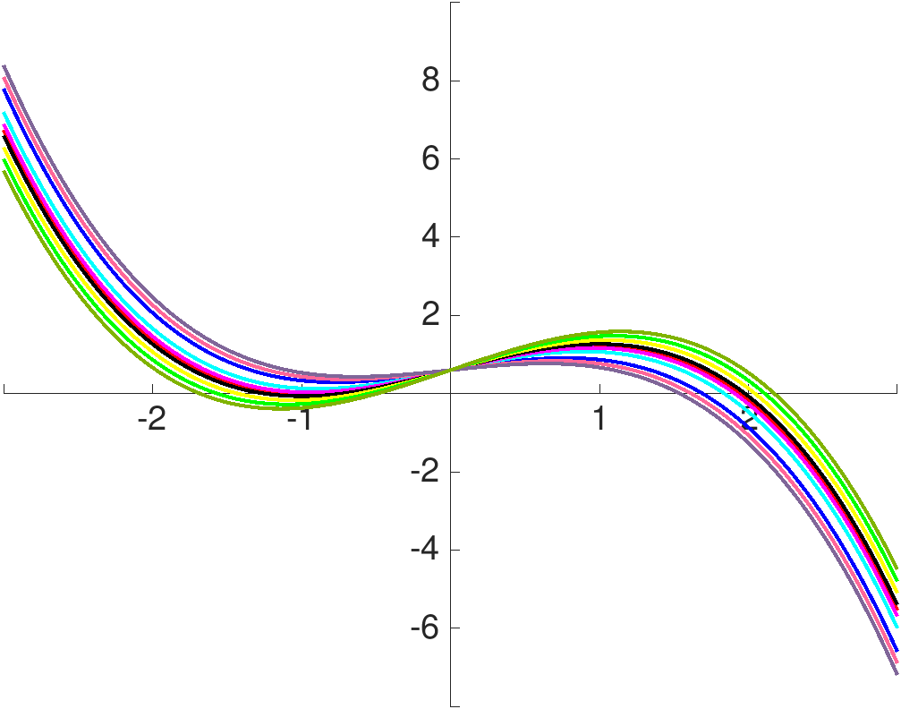
(a)

Figure 1: Graph of $g(z)=\tau+\alpha z-\displaystyle\frac{z^{3}}{3}$ for different parameter values of $\alpha$ and fixed $\tau=0.6$.

For all $\alpha\in\mathbb{R}$ Equation (1) has at exactly one equilibrium solution with $x=y=0$ and $z>0$, which we denote by $p_{0}\in\mathbb{R}^{3}$. This equilibrium has one stable eigenvalue, whose eigenvector coincides with the $z$-axis. The remaining eigenvalues are complex conjugate unstable. At $\alpha\approx 0.9321697517861$ there is a saddle node bifurcation giving rise to a new pair of equilibrium points $p_{1},p_{2}\in\mathbb{R}^{3}$. These equilibria persist for all larger values of $\alpha$. One of the equilibrium points appearing out of the saddle node bifurcation is fully stable, with three eigenvalues having negative real parts, and we denote it by $p_{2}\in\mathbb{R}^{3}$. The other new equilibrium, which we denote by $p_{1}\in\mathbb{R}^{3}$, is a saddle-focus with a complex conjugate pair of stable eigenvalues and one real unstable eigenvalue. The unstable eigenvector again coincides with the $z$-axis. Indeed, since the $z$-axis is invariant, the stable manifold of $p_{0}$ and the unstable manifold of $p_{1}$ coincide, and are contained in the $z$-axis. This intersection is not transverse, and is rather forced by a rotational symmetry of the problem.

Now consider the plane $z=\beta$, and note that when the field is projected onto this plane the nonlinear terms vanish from the first two components giving a pure rotation. The plane is however not invariant, as $z^{\prime}$ does not vanish there. Nevertheless there is a periodic orbit $\gamma$ near the $z=\beta$ plane. This periodic orbit, and the invariant $z$ axis organize the dynamics of the system. The vector field along with the periodic orbit and the dynamics on the $z$-axis are illustrated in the left frame of Figure 2.

As we will see below, the periodic orbit $\gamma$ has a pair of complex conjugate Floquet exponents, hence solutions of the differential equation tend to circulate around $\gamma$. The orbit may be either attracting or repelling depending on the value of $\alpha$. This circulation about the periodic orbit is a dominant feature of the dynamics.

Further insight into the dynamics is obtained by numerically integrating some trajectories (phase space sampling), as was done in the work of Langford [20]. We provide, for the sake of completeness, the results of a few such simulations. The results illustrated in Figure 3 make clear the typical behavior of the system, and suggest the existence of a “torus-like” attractor. Simulations were run for roughly one hundred time units. The periodic orbit $\gamma$ runs through the center of the torus but is, as we will see, repelling for these parameter values. The saddle focus points $p_{0}$ and $p_{1}$ are at the top and bottom of the torus.

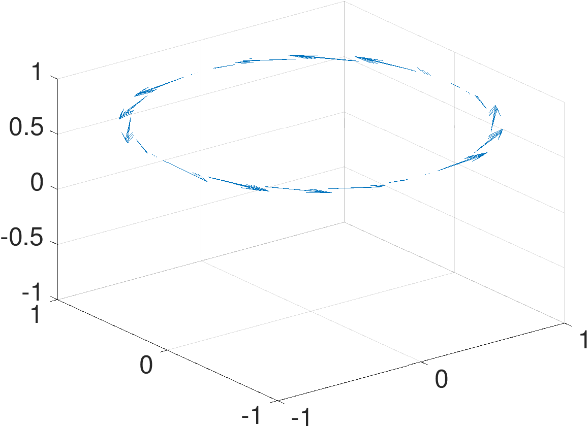
(a)

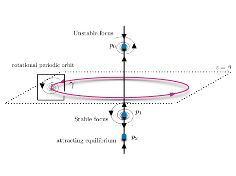
(b)

Figure 2: Phase space geography: the main features of the system are the invariance of the $z$-axis, the rotation in the $z=\beta$ plane leading to a periodic orbit, and the unstable saddle focus at $p_{0}$. The periodic orbit $\gamma$ is located near (but does not sit on) the $z=\beta$ plane. The periodic orbit has complex conjugate Floquet multipliers which are stable for small $\alpha$ but which later cross the unit circle, loosing stability in a Neimark-Sacker bifurcation. For some $\alpha$ values there are an additional pair of equilibria $p_{1}$– stable focus and $p_{2}$ – attracting point. This situation is illustrated in the schematic on the right. Left: the phase portrait of the vector field along the periodic orbit.

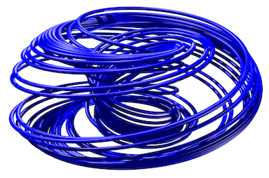
(a) $\alpha=0.8$

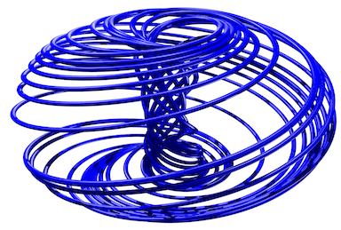
(b) $\alpha=0.95$

Figure 3: Direct simulation: For many values of the bifurcation parameter $\alpha$ the system appears to have an attractor with torus-like dynamics (product of two circles). This is caused by circulation due to the complex conjugate Floquet exponents of the periodic orbit, and generates a kind of “vortex”.

1.2 Some remarks on the literature

Roughly speaking, the dynamics described above suggests the system as a toy model for dissipative vortex dynamics, or for a rotating viscus fluid. There is a rich literature on the dynamics of vortex bubbles, and the interested reader might consult the works of [14, 28, 29, 30, 31] for a more thorough discussion of the literature. We remark that the torus bifurcations seen in the Langford system are similar to those seen in the piecewise linear electronic circuit of [32], the commodity distribution model of [33], and the mechanical oscillators of [34, 35] to name only a few. The appearance and destruction of invariant tori, as well as resonance phenomena and routes to chaos are discussed much more generally in [5, 36] and the references found therein.

One further remark is in order. The system given by Equation (1) has been called the Aizawa system by some researchers, and is the subject of some other recent work on visualization. For example researchers interested in computer animation [37], three dimensional printing [38], and even in graphical arts [39] have made interesting studies and use this name for the equations. This nomenclature seems to be a misnomer, as the equations do not appear in the works of Yoji Aizawa, and a more appropriate name for Equation (1) would seem to be the Langford system, due to the fact that – as already mentioned above – the system was proposed in [20].

2 Review of the parameterization method

The parameterization method is a general functional analytic framework for studying invariant manifolds of discrete and continuous time dynamical systems, first developed in [25, 26, 27] in the context of stable/unstable manifolds attached to fixed points of nonlinear mappings on Banach spaces, and later extended in [40, 41, 42] for studying whiskered tori. There is a thriving literature devoted to computational applications of the parameterization method, and the interested reader may want to consult [10, 18, 19, 43, 44, 45, 46, 47, 48, 49, 50, 51, 52, 53, 54], though the list is far from being exhaustive. A much more complete discussion is found in the book [55].

This section provides a practical overview of the parameterization method with a strong emphasis on numerical aspects utilized in the sequel. The discussion focuses on analytic vector fields, and requisite formal series calculations are carried out for the specific example of Equation (1). Since this material is not completely standard outside a certain circle of practitioners, it is included primarily so that the present work stands alone for a broad readership. The reader either already familiar with or uninterested in these developments is encouraged to skip ahead to Section 3, referring back to this section only as needed.

The Langford system admits equilibrium solutions with complex eigenvalues, so that it is best to present the entire theory for complex vector fields. Later we explain how to recover parameterizations of real invariant manifolds associated with complex conjugate eigenvalues of real vector fields. So, let $f\mathrel{\mathop{\mathchar 58\relax}}\mathbb{C}^{k}\to\mathbb{C}^{k}$ be an analytic vector field and $\hat{p}\in\mathbb{C}^{k}$ have $f(\hat{p})=0$ so that $x(t)=\hat{p}$ is an equilibrium solution of the differential equation $x^{\prime}=f(x)$. Assume for the sake of simplicity that $Df(\hat{p})$ is diagonalizable over $\mathbb{C}$ having $k_{s}$ stable (and $k_{u}$ unstable) eigenvalues of multiplicity one. We do not necessarily assume that $k_{s}+k_{u}=k$, that is we do not rule out the possibility of some center directions at $\hat{p}$ (though this situation will not occur in the present work).

Label the stable eigenvalues as $\lambda_{1}^{s},\cdots,\lambda_{k_{s}}^{s}$ and the unstable ones as $\lambda_{1}^{u},\cdots,\lambda_{k_{u}}^{u}$ and order them according to the convention that

$$\textrm{real}(\lambda_{1}^{s})\leq\cdots\leq\textrm{real}(\lambda_{k_{s}}^{s})<0<\textrm{real}(\lambda_{1}^{u})\leq\cdots\leq\textrm{real}(\lambda_{k_{u}}^{u}).$$

Since $Df(\hat{p})$ is diagonalizable there are linearly independent eigenvectors $\xi_{1}^{u},\cdots,\xi_{k_{u}}^{u}\in\mathbb{C}^{k}$ and $\xi_{1}^{s},\cdots,\xi_{k_{s}}^{s}\in\mathbb{C}^{k}$ associated with the unstable and stable eigenvalues respectively.

Remark 2.1.

The assumption that $Df(\hat{p})$ is diagonalizable is made only for the sake of convenience. See [25] for a much more general theoretical setup. See also [47] for a complete description of the functional analytic set up and examples of the numerical implementation when there are repeated eigenvalues. Nevertheless, the assumption holds in the examples considered throughout the present work.

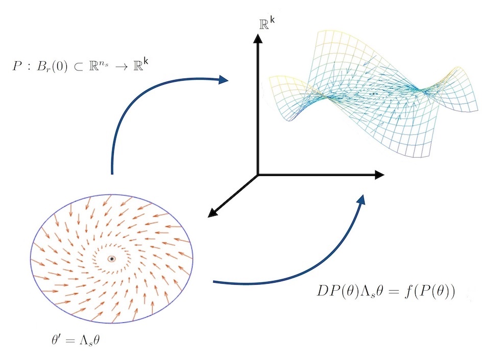
Figure 4: Geometry of the parameterization method: the push forward of the linear vector field $\Lambda_{s}\theta$ by $P$ is equal to the given vector field $f$ restricted to the image of $P$. Then the dynamics on the image of $P$ are conjugate to the linear dynamics generated by $\Lambda_{s}\theta$.

2.1 Invariance equation

Given the setup introduced in the previous section we are interested in computing an accurate representation of the $k_{s}$ dimensional local stable manifold attached to $\hat{p}$. The parameterization method seeks a smooth surjective map $P$ satisfying the first order system of partial differential equations

$$\lambda^{s}_{1}\theta_{1}\frac{\partial}{\partial\theta_{1}}P(\theta_{1},\ldots,\theta_{k_{s}})+\ldots+\lambda^{s}_{k_{s}}\theta_{k_{s}}\frac{\partial}{\partial\theta_{k_{s}}}P(\theta_{1},\ldots,\theta_{k_{s}})=f(P(\theta_{1},\ldots,\theta_{k_{s}})),$$ (2)

for $\theta=(\theta_{1},\ldots,\theta_{k_{s}})\in\mathbb{C}^{k_{s}}$, and subject to the first order constraints

$$P(0,\ldots,0)=\hat{p},\quad\quad\quad\mbox{and}\quad\quad\quad\frac{\partial}{\partial\theta_{j}}P=\xi^{s}_{j},\quad\quad 1\leq j\leq k_{s}.$$ (3)

Equation (2) is referred to as the invariance equation for $P$. A map $P$ solving Equation (2) subject to the first order constraints of Equation (3) is a parameterization of the local stable manifold, as we explain below. Making the obvious adjustments for the unstable eigenvalues/eigenvectors leads to a parameterization method for the $k_{u}$ dimensional unstable manifold.

To explain the meaning of Equation (2), let

$$\Lambda_{s}=\left(\begin{array}[]{ccc}\lambda_{1}&\ldots&0\\ \vdots&\ddots&\vdots\\ 0&\ldots&\lambda_{k_{s}}\end{array}\right),$$

so that the invariance equation becomes

$$DP(\theta)\Lambda_{s}\theta=f(P(\theta)).$$

In the language of differential geometry, this equation says that the push forward by $P$ of the linear vector field $\Lambda_{s}\theta$ is equal to the vector field $f$ restricted to the image of $P$. Where the vector fields are equal they generate the same dynamics. But the dynamics generated by $\Lambda_{s}\theta$ are completely understood: all orbits converge exponentially to the origin. It follows that all orbits on the image of $P$ converge to $\hat{p}$. Since the image of $P$ is a smooth $k_{s}$ dimensional disk, it is a local stable manifold for $\hat{p}$. The situation is illustrated in Figure 4.

The observation is made more precise as follows. Denote by $\phi\colon\mathbb{C}^{k}\times\mathbb{C}\to\mathbb{C}^{k}$ the flow generated by $f$. The flow generated by $\Lambda_{s}\theta$ is given explicitly by

$$L(\theta,t)=e^{\Lambda_{s}t}\theta.$$

One checks that $P$ satisfies Equation (2) if and only if

$$\phi\left(P(\theta),t\right)=P\left(e^{\Lambda_{s}t}\theta\right),$$ (4)

for all $t\geq 0$. This flow conjugacy is illustrated in Figure 5. Elementary proofs of these claims are found in any of the references [48, 55, 56]. Moreover, replacing the stable by the unstable eigenvalues and eigenvectors in the discussion above and reversing time, the entire discussion carries through for the unstable manifold.

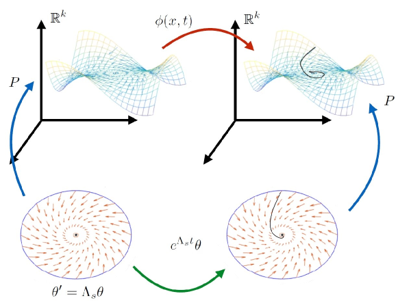
Figure 5: Flow conjugacy: a mapping $P$ satisfying the invariance equation (2) has that the diagram above commutes.

Remark 2.2 (Real analytic vector fields and manifolds).

If $f\colon\mathbb{R}^{k}\to\mathbb{R}^{k}$ is a real analytic vector field with a real equilibrium $\hat{p}\in\mathbb{R}^{k}$ then the discussion above applies to an analytic extension of the vector field in a neighborhood of $\hat{p}$. In this case any complex eigenvalues of $Df(\hat{p})$ appear in complex conjugate pair, and the associated eigenvectors can be taken complex conjugate. We look for a solution $P$ of Equation (2) taking real values on complex conjugate variables. This condition imposes a symmetry on the Taylor coefficients of the parameterization $P$, as illustrated explicitly in the examples below.

2.2 Formal series solution of Equation (2) for the Langford system

In this section we further restrict to the case of interest in the present work, where $\hat{p}\in\mathbb{C}^{3}$ and $\lambda_{1},\lambda_{2}\in\mathbb{C}$ are a pair of stable (or unstable) complex conjugate eigenvalues and $\lambda_{3}$ has the opposite stability. Let $\xi_{1},\xi_{2}\in\mathbb{C}^{3}$ be an associated pair of linearly independent complex conjugate eigenvectors. Since the field is analytic, we look for an analytic parameterization

$$P(\theta_{1},\theta_{2})=\sum_{m=0}^{\infty}\sum_{n=0}^{\infty}\begin{pmatrix}p_{mn}^{1}\\ p_{mn}^{2}\\ p_{mn}^{3}\\ \end{pmatrix}\theta_{1}^{m}\theta_{2}^{n},$$

satisfying Equation (2), which in this case is reduced to

$$\lambda_{1}\theta_{1}\frac{\partial}{\partial\theta_{1}}P(\theta_{1},\theta_{2})+\lambda_{2}\theta_{2}\frac{\partial}{\partial\theta_{2}}P(\theta_{1},\theta_{2})=f(P(\theta_{1},\theta_{2})),$$

where $f\colon\mathbb{C}^{3}\to\mathbb{C}^{3}$ is the Langford vector field given in Equation (1). Here $p_{mn}^{j}\in\mathbb{C}$ for all $j=1,2,3$. Imposing the linear constraints of Equation (3) gives that $p_{00}=\hat{p}$, $p_{10}=\xi_{1}$ and $p_{01}=\xi_{2}$.

Now we would like to expand Equation (2) in terms of the power series. The left hand side of Equation (2) is

$$\lambda_{1}\theta_{1}\frac{\partial}{\partial\theta_{1}}P(\theta_{1},\theta_{2})+\lambda_{2}\theta_{2}\frac{\partial}{\partial\theta_{2}}P(\theta_{1},\theta_{2})=\sum_{m=0}^{\infty}\sum_{n=0}^{\infty}(m\lambda_{1}+n\lambda_{2})p_{mn}\theta_{1}^{m}\theta_{2}^{n},$$

on the level of power series. To expand the right hand side we begin by writing

$$P_{j}(\theta_{1},\theta_{2})=\sum_{m=0}^{\infty}\sum_{n=0}^{\infty}p_{mn}^{j}\theta_{1}^{m}\theta_{2}^{n},$$

for $j=1,2,3$ to denote the component power series. The field contains the nonlinear terms $zx$, $zy$, $z^{3}$, $x^{2}z$, $y^{2}z$, and $zx^{3}$ (see again Equation (1)). Computing the power series for $f\circ P$ requires expanding these monomials of components of $P$, which is accomplished using Cauchy products. For example the coefficients of $P_{3}\cdot P_{1}$ are

$$(p^{3}*p^{1})_{mn}=\sum_{j=0}^{m}\sum_{k=0}^{n}p_{(m-j)(n-k)}^{3}p_{jk}^{1},$$

while the coefficients of $P_{3}\cdot P_{1}^{3}$ are

$$(p^{3}*p^{1}*p^{1}*p^{1})_{mn}=\sum_{i_{1}=0}^{m}\sum_{i_{2}=0}^{i_{1}}\sum_{i_{3}=0}^{i_{2}}\sum_{k_{1}=0}^{n}\sum_{k_{2}=0}^{k_{1}}\sum_{k_{3}=0}^{k_{2}}p_{(m-i_{1})(n-k_{1})}^{3}p_{(i_{1}-i_{2})(k_{1}-k_{2})}^{1}p_{(i_{2}-i_{3})(k_{2}-k_{3})}^{1}p_{i_{3}k_{3}}^{1}.$$

Other products are similar.

Substituting these power series expansions into the invariance equation (2) and matching like powers of $\theta_{1}$ and $\theta_{2}$ leads to

$$(m\lambda_{1}+n\lambda_{1})\left[\begin{array}[]{c}p_{mn}^{1}\\ p_{mn}^{2}\\ p_{mn}^{3}\end{array}\right]=$$ (5)

$${\tiny\left[\begin{array}[]{c}(p^{3}*p^{1})_{mn}-\beta p_{mn}^{1}-\delta p_{mn}^{2}\\ (p^{3}*p^{2})_{mn}-\beta p_{mn}^{2}+\delta p_{mn}^{1}\\ \alpha p_{mn}^{3}-\displaystyle\frac{1}{3}(p^{3}*p^{3}*p^{3})_{mn}-(p^{1}*p^{1})_{mn}-(p^{2}*p^{2})_{mn}-\varepsilon(p^{1}*p^{1}*p^{3})_{mn}-\varepsilon(p^{2}*p^{2}*p^{3})_{mn}+\zeta(p^{1}*p^{3}*p^{3}*p^{3})_{mn}\end{array}\right],}$$

for $m+n\geq 2$. To isolate terms of order $(m,n)$ consider that

$$(p^{3}*p^{1})_{mn}=p_{00}^{3}p_{mn}^{1}+p_{00}^{1}p_{mn}^{3}+(p^{3}\hat{*}p^{1})_{mn},$$ (6)

where

$$(p^{3}\hat{*}p^{1})_{mn}=\sum_{j=0}^{m}\sum_{k=0}^{n}\hat{\delta}_{jk}^{mn}p_{(m-j)(n-k)}^{3}p_{jk}^{1},$$

and

$$\hat{\delta}_{jk}^{mn}=\begin{cases}0&\mbox{if }j=k=0\\ 0&\mbox{if }j=m\mbox{ and }k=n\\ 1&\mbox{otherwise}\end{cases}.$$

The point here is that $(p^{3}\hat{*}q^{1})_{mn}$ is precisely the sum left when terms containing $p_{mn}$ are extracted from the Cauchy product.

This expression is directly related to the derivative of $f$. To see this, let

$$g(x,z)=xz,$$

and note that Equation (6) becomes

$$(g\circ P)_{mn}=\nabla g(p_{00}^{1},p_{00}^{3})\left[\begin{array}[]{c}p_{mn}^{1}\\ p_{mn}^{3}\end{array}\right]+(p^{1}\hat{*}p^{3})_{mn}.$$

Using this notation the first component of Equation (5) is

$$(m\lambda_{1}+n\lambda_{2})p_{mn}^{1}=\nabla g(p_{00}^{1},p_{00}^{3})\left[\begin{array}[]{c}p_{mn}^{1}\\ p_{mn}^{3}\end{array}\right]+(p^{1}\hat{*}p^{3})_{mn}-\beta p_{mn}^{1}-\delta p_{mn}^{2}.$$

Isolating terms of order $(m,n)$ on the left and lower order terms on the right gives

$$\nabla g(p_{00}^{1},p_{00}^{3})\left[\begin{array}[]{c}p_{mn}^{1}\\ p_{mn}^{3}\end{array}\right]-\beta p_{mn}^{1}-\delta p_{mn}^{2}-(m\lambda_{1}+n\lambda_{2})p_{mn}^{1}=-(p^{1}\hat{*}p^{3})_{mn},$$

which is linear in $p_{mn}^{1}$. Comparing the right hand side in the equation above with the vector field $f$, and recalling that $\hat{p}=p_{00}$, we see that

$$\nabla g(p_{00}^{1},p_{00}^{3})\left[\begin{array}[]{c}p_{mn}^{1}\\ p_{mn}^{3}\end{array}\right]-\beta p_{mn}^{1}-\delta p_{mn}^{2}=\nabla f_{1}(\hat{p})\left[\begin{array}[]{c}p_{mn}^{1}\\ p_{mn}^{3}\end{array}\right].$$

Combining the equation above with a nearly identical computation for the second component, and a somewhat lengthier computation for the third component, and noting that

$$Df(\hat{p})=\left[\begin{array}[]{c}\nabla f_{1}(\hat{p})\\ \nabla f_{2}(\hat{p})\\ \nabla f_{3}(\hat{p})\end{array}\right],$$

we obtain the expansion

$$(f\circ P)_{mn}=Df(\hat{p})p_{mn}+$$

$${\tiny\left[\begin{array}[]{c}(p^{3}\hat{*}p^{1})_{mn}\\ (p^{3}\hat{*}p^{2})_{mn}\\ -\displaystyle\frac{1}{3}(p^{3}\hat{*}p^{3}\hat{*}p^{3})_{mn}-(p^{1}\hat{*}p^{1})_{mn}-(p^{2}\hat{*}p^{2})_{mn}-\varepsilon(p^{1}\hat{*}p^{1}\hat{*}p^{3})_{mn}-\varepsilon(p^{2}\hat{*}p^{2}\hat{*}p^{3})_{m}n+\zeta(p^{1}\hat{*}p^{3}\hat{*}p^{3}\hat{*}p^{3})_{mn}\end{array}\right].}$$

Substituting this expansion into Equation (5) gives

$$(m\lambda_{1}+n\lambda_{2})p_{mn}=Df(\hat{p})p_{mn}+$$

$${\tiny\left[\begin{array}[]{c}(p^{3}\hat{*}p^{1})_{mn}\\ (p^{3}\hat{*}p^{2})_{mn}\\ -\displaystyle\frac{1}{3}(p^{3}\hat{*}p^{3}\hat{*}p^{3})_{mn}-(p^{1}\hat{*}p^{1})_{mn}-(p^{2}\hat{*}p^{2})_{mn}-\varepsilon(p^{1}\hat{*}p^{1}\hat{*}p^{3})_{mn}-\varepsilon(p^{2}\hat{*}p^{2}\hat{*}p^{3})_{m}n+\zeta(p^{1}\hat{*}p^{3}\hat{*}p^{3}\hat{*}p^{3})_{mn}\end{array}\right],}$$

and by isolating terms of order $(m,n)$ on the left we obtain the linear homological equations

$$[Df(\hat{p})-(m\lambda_{1}+n\lambda_{2})\mbox{Id}]p_{mn}=s_{mn},$$ (7)

for $p_{mn}$, where

$$s_{mn}=\left(\begin{array}[]{c}s_{mn}^{1}\\ s_{mn}^{2}\\ s_{mn}^{3}\end{array}\right),$$

with

$$s_{mn}^{1}=-(p^{3}\hat{*}p^{1})_{mn},$$

$$s_{mn}^{2}=-(p^{3}\hat{*}p^{2})_{mn},$$

and

$$s_{mn}^{3}=$$

$$\frac{1}{3}(p^{3}\hat{*}p^{3}\hat{*}p^{3})_{mn}+(p^{1}\hat{*}p^{1})_{mn}+(p^{2}\hat{*}p^{2})_{mn}+\varepsilon(p^{1}\hat{*}p^{1}\hat{*}p^{3})+\varepsilon(p^{2}\hat{*}p^{2}\hat{*}p^{3})-\zeta(p^{1}\hat{*}p^{1}\hat{*}p^{1}\hat{*}p^{3})_{mn}.$$

We make the following observations:

• While our derivation of Equation (7) is particular to the Langford system of Equation (1), we remark that the form of the homological equations is always the same. Only the right hand side depends on the particular nonlinearity of the given system.

• The matrix acting on $p_{mn}$ is the characteristic matrix for the differential at $\hat{p}$. Then the equation is uniquely solvable at order $(m,n)$ if $m\lambda_{1}+n\lambda_{2}$ is not an eigenvalue.

• Since $\lambda_{3}$ has the opposite stability of $\lambda_{1},\lambda_{2}$, we obtain the non-resonance condition

  $$m\lambda_{1}+n\lambda_{2}\neq\lambda_{j},\quad\quad\quad j=1,2.$$

  If the non-resonance conditions are satisfied for all $m,n\in\mathbb{N}$ with $m+n\geq 2$, then the formal series solution of Equation (2) is formally well defined to all orders.

• If $\lambda_{2}=\overline{\lambda_{1}}$, that is if we consider the complex conjugate case, then there is no possibility of a resonance and we can compute the power series coefficients of the parameterization to any desired finite order.

• When $\lambda_{1},\lambda_{2}$ are complex conjugates, the coefficients of $P$ have the symmetry $\overline{p_{nm}}=p_{mn}$ for all $m+n\geq 2$. This is seen by taking complex conjugates of both sides of the homological equation, and using the fact that $Df(\hat{p})$ is a real matrix.

  Since $\hat{p}$ is real, choosing complex conjugate eigenvectors $\xi_{2}=\overline{\xi_{1}}$ enforces the symmetry to all orders. The power series solution $P$ has complex coefficients, but we obtain the real image of $P$ by taking complex conjugate variables. That is, we define for the real parameters $s_{1},s_{2}$ the function

  $$\hat{P}(s_{1},s_{2})=P(s_{1}+is_{2},s_{1}-is_{2}),$$

  which parameterizes the real stable/unstable manifold.

2.3 Numerical considerations

The homological equations derived in the previous section allow us to recursively compute the power series coefficients of the stable/unstable manifold parameterization $P$ to any desired order $m+n=N$. The coefficients are uniquely determined up to the choice of the scaling of the eigenvectors. In practical applications we have to decide how to answer the following questions:

• To what order $N$ will we compute the approximate parameterization?

• What scale to choose for the eigenvectors?

• On what domain do we to restrict the polynomial $P^{N}$?

In practice we proceed as follows. First we choose a convenient value for $N$, based on how long we want to let the computations run. Then, we always restrict $P$ to the unit disk for the sake of numerical stability. Finally, we choose the eigenvector scaling so that the last coefficients, the coefficients of order $N$, are smaller than some prescribed tolerance. A good empirical rule of thumb is that the truncation error is roughly the same magnitude as the $N$-th order coefficients.

In practice we can prescribe the size of the $N$-th order terms as soon as we know the exponential decay rate of the coefficients. In the next section we describe the relationship between the scale of the eigenvectors and the exponential decay rate.

2.3.1 Rescaling the eigenvectors

In Section 2.2 we saw that the power series coefficients of the parameterization are uniquely determined up to the choice of the eigenvector. Since the eigenvectors are unique up to the choice of length, we have that the length determines uniquely the coefficients. In fact the effect of rescaling the eigenvectors is made completely explicit as follows. The material in this section is discussed in greater detail in [46].

Suppose that

$$P(\theta_{1},\theta_{2})=\sum_{m=0}^{\infty}\sum_{n=0}^{\infty}p_{mn}\theta_{1}^{m}\theta_{2}^{n},$$

is the formal solution of Equation (2), with

$$p_{00}=\hat{p},\quad\quad\quad p_{10}=\xi_{1},\quad\quad\quad\mbox{and}\quad\quad\quad p_{01}=\xi_{2},$$

where $\|\xi_{1}\|=\|\xi_{2}\|=1$. Assuming that $P$ is bounded and analytic on the complex poly-disk with radii $R_{1},R_{2}>0$, there is a $C>0$ so that

$$|p_{mn}|\leq\frac{C}{R_{1}^{m}R_{2}^{n}},$$

by the Cauchy estimates.

Now choose non-zero $s_{1},s_{2}\in\mathbb{R}$ and define the rescaled eigenvectors

$$\eta_{1}=s_{1}\xi_{1},\quad\quad\quad\mbox{and}\quad\quad\quad\eta_{2}=s_{2}\xi_{2}.$$

The new parameterization associated with the rescaled eigenvectors is given by

$$Q(\theta_{1},\theta_{2})=\sum_{m=0}^{\infty}\sum_{n=0}^{\infty}q_{mn}\theta_{1}^{m}\theta_{2}^{n},$$

where

$$q_{mn}=s_{1}^{m}s_{2}^{n}p_{mn}.$$ (8)

See [46] for a proof of this identity, and also the discussion in [25, 27]. The coefficients of the rescaled parameterization have the new exponential decay rate given by

$$|q_{mn}| =\left|s_{1}^{m}s_{2}^{m}p_{mn}\right|$$

$$\leq s_{1}^{m}s_{2}^{n}\frac{C}{R_{1}^{m}R_{2}^{n}}$$

$$\leq\frac{C}{\left(\frac{R_{1}}{s_{1}}\right)^{m}\left(\frac{R_{2}}{s_{2}}\right)^{n}}.$$

These observations lead to a practical algorithm. First compute the parameterization $P$ with an arbitrary choice of eigenvector scaling (for example scaled to have length one). Then solve the homological equations to some order $N_{0}$ using this scaling, and compute $C$, $R_{1}$ and $R_{2}$ using an exponential best fit. Suppose that $\varepsilon_{0}>0$ is the desired tolerance, that is the desired size of the order $N\geq N_{0}$ coefficients. Then we choose $s_{1}$ and $s_{2}$ so that

$$\frac{C}{\left(\frac{R_{1}}{s_{1}}\right)^{N}\left(\frac{R_{2}}{s_{2}}\right)^{N}}\leq\varepsilon_{0}.$$

Finally we recompute the coefficients $q_{mn}$ for $2\leq m+n\leq N$. The rescaled coefficients could be computed from the old coefficients using the formula of Equation (8). In practice however better results are obtained by recomputing the coefficients $q_{mn}$ from scratch via the homological equations.

We remark that in the case of complex conjugate eigenvalues we want the eigenvectors to be complex conjugates. Assuming that $\xi_{2}=\overline{\xi}_{1}$ we take $s_{1}=s_{2}\in\mathbb{R}$ so that $\eta_{2}=\overline{\eta}_{1}$. Also note that by choosing our domain to be the unit poly-disk, we have that $R_{1}=R_{2}=1$, further simplifying the analysis.

2.3.2 A-posteriori error

Once we have chosen the polynomial order $N$ and the scaling of the eigenvectors, that is once we have uniquely specified our parameterization to order $N$, we would like a convenient measure of the truncation error. As mentioned above, a good heuristic indicator is that the error is roughly the size of the highest order coefficients (assuming we take the unit disk as the domain of our approximate parameterization). In this section we discuss a more quantitative indicator.

We remark that there exist methods of a-posteriori error analysis for the parameterization method, which – when taken to their logical conclusion – lead to mathematically rigorous computer assisted error bounds on the truncation errors. The interested reader will find fuller discussion and more references to the literature in [27, 46, 47, 55, 56, 57] and discussion of related techniques in [58, 59, 60].

The analysis in the present work is qualitative and we don’t require the full power of mathematically rigorous error bounds. Instead we employ an error indicator inspired by the fact that the parameterization satisfies the flow invariance property given in Equation (4). We choose $T{\not=}0$, and a partition of the interval $[0,2\pi]$ into $K$ angles, $\alpha_{j}=2\pi j/(K+1)$, for $0\leq j\leq K$. Since we are interested in the case of complex conjugate eigenvalues $\lambda,\overline{\lambda}\in\mathbb{C}$, we define complex conjugate parameters

$$\theta_{j}=(\theta_{1}^{j}+i\theta_{2}^{j},\theta_{1}^{j}-i\theta_{2}^{j})=(\cos(\alpha_{j})+i\sin(\alpha_{j}),\cos(\alpha_{j})-i\sin(\alpha_{j})),$$

and the linear mapping

$$e^{\Lambda T}=\left(\begin{array}[]{cc}e^{\lambda T}&0\\ 0&e^{\overline{\lambda}T}\end{array}\right).$$

which maps complex conjugate inputs to complex conjugate outputs. The a-posteriori indicator is

$$\mbox{Error}_{\mbox{{\tiny conj}}}\left(N,T\right)=\max_{0\leq j\leq K}\left\|\phi(P^{N}(\theta_{j}),T)-P^{N}(e^{\Lambda T}\theta_{j})\right\|.$$

Here $T>0$ if the complex conjugate eigenvalues $\lambda,\overline{\lambda}$ are stable and $T<0$ if they are unstable. In practice the flow map $\phi(x,t)$ will be evaluated using a numerical integration scheme, and the accuracy of the indicator is limited by the accuracy of the integrator.

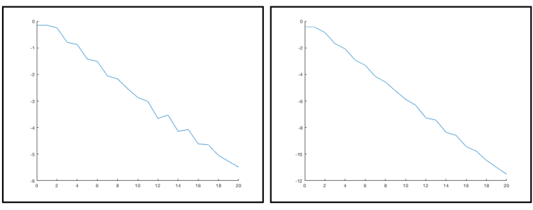
Figure 6: Rescaling the eigenvector and coefficient decay: the left frame shows the coefficient decay when the eigenvectors are scaled to unit length. The right frame is with scaling one half. Both figures plot coefficient magnitude $\max_{i+j=n}\log(|p_{ij}|)$ (vertical axis) versus polynomial order $n$ (horizontal axis). When the eigenvector is scaled to unit length we see that the order 20 coefficient are on the order of $10^{-6}$, which is small but far from machine epsilon. We should either increase the order of the polynomial or decrease the scale of the eigenvector. Indeed, when the scale is decreased to one half we see that the last coefficients have magnitude on the order of a few thousand multiples of machine epsilon.

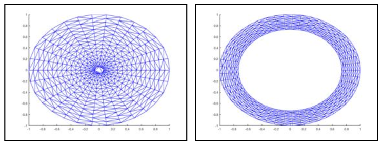
Figure 7: Triangulating the local invariant manifold and fundamental domain: for the local parameterization we subdivide the unit disk – fifteen radial subdivisions by 30 angular subdivisions (left). Since the domain is simply connected, the triangulation is computed using Delauney’s algorithm (built into MATLAB). For a fundamental domain we take the unit circle as the outer boundary, and the circle of radius $|e^{-\lambda_{u}\tau}|$ as the inner boundary of an annulus. We take ten radial subdivisions and fifty angular subdivisions. We compute a Delauney triangulation, but this “fills in the hole” of the annulus. This is fixed by removing triangles with a long side from the triangulation and results in the mesh illustrated in the right.

2.3.3 A numerical example

As an example of the performance of the method, consider the parameterization of the two dimensional unstable manifold of the Langford system (Equation (1)) at the equilibirum $p_{0}$, computed to order $N=20$. Figure 6 illustrates the effect of the choice of the eigenvector scaling on the decay rate of the Taylor coefficient. We remark that the magnitude of the last Taylor coefficient computed is a good heuristic indicator of the size of the truncation error. For example if we choose eigenvectors scaled to length one, we obtain the decay rate illustrated in the left frame of Figure 6, and we see that the norm of the largest coefficient of order twenty is about $10^{-6}$. On the other hand if we rescale to eigenvector to have length $1/2$ then the coefficients decay as in the right frame of Figure 6, and the largest norm of any coefficient of order twenty is now about $10^{-12}$.

To visualize the parameterized local manifold we evaluate the polynomial approximation on the unit disk. First we take a Delaunay triangulation of the unit disk as illustrated in the left frame of Figure 7. This triangulation of the unit disk is pushed forward to the phase space $\mathbb{R}^{3}$ by the polynomial parameterization, resulting in a triangulation of the two dimensional local unstable manifold as illustrated in the top left frame of Figure 8.

To “grow” a larger representation of the unstable manifold we choose a fundamental domain, for example by taking $\tau=0.25$ and considering the annulus in parameter space formed by the boundary of the unit disk and by the circle of radius $R=\left|e^{\lambda_{u}\tau}\right|\approx 0.733$. We mesh this annulus using $100$ angular subdivisions and $40$ radial subdivisions, as illustrated in the right frame of Figure 7. We lift this fundamental domain to the phase space and repeatedly apply the time $\tau=0.25$ map via numerical integration of the vertices of the triangulation. We refine the mesh whenever any side of a triangle in phase space gets too large. In the present work we measure “too large” just by looking at the resulting picture.

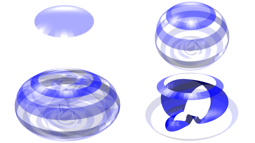
Figure 8: Growing the unstable manifold one fundamental domain at a time: (Top left) the initial local unstable manifold obtained using the parameterization method. (Top right) the initial local manifold parameterization as well as the first, third, fifth, seventh, ninth, eleventh, thirteenth, and fifteenth iterate of the fundamental domain. (Bottom left) the first through thirty third iterates of the fundamental domain. (Bottom right) the sixtieth iterate of the fundamental domain, and we see that the image is substantially folded. The first and sixth iterates are shown as well to provide the overall shape of the bubble. In the bottom frames the initial parameterized local unstable manifold is not shown.

The top right, and bottom frames of Figure 8 illustrate the results of iterating a triangulation of a fundamental domain for the local unstable manifold at $p_{0}$, and we see that the “bubble” grows in a quite regular way. However, by the time we take $60$ iterates the embedding of the initial annulus is becoming quite complicated.

2.4 Numerical approximation methods for stable/unstable manifolds

The literature devoted to numerical approximation of stable/unstable manifolds is substantial, and we take a moment to reframe the techniques just discussed in this light. A classic general reference is the work of [61]. The essential remark is that computational methods for studying stable/unstable manifolds decompose naturally into two independent tasks:

• Step 1: Calculate an approximation of the local invariant manifold.

• Step 2: Advect the local approximation, “growing” the representation of the manifold.

A natural approach to Step 1 is to approximate the local manifold to first order, reducing the problem to linear algebra. That is, by computing the eigenvalues/eigenvectors of the differential at the equilibrium we can approximate the local stable/unstable manifolds by the stable/unstable eigenspaces. Step 2 is in general much more difficult, due to the fact that nonlinearities cause the manifold to grow in a highly nonuniform way. For this reason, much work focuses on the development of powerful methods for Step 2. We refer the interested reader to the works of [62, 63, 64, 65, 66, 66, 67, 68, 69], and also to the survey paper of [70] for much fuller discussion of the topic. The woks just cited develop sophisticated adaptive subdivision schemes to control the accuracy and complexity of the advection problem, growing the stable/unstable manifolds in a uniform way.

Another way to fight the nonuniformity encountered at Step 2 is to employ a higher order approximation scheme, and hence to compute a larger portion of the stable/unstable manifold at Step 1. The idea is that a manifold approximation holding in a large neighborhood of the equilibrium reduces the dramatic expansion which results from integrating a very small polygonal manifold patch until it describes a large portion of the manifold.

The parameterization method as discussed in the present section accomplishes this. Indeed, deriving the homological equations for the system facilitates the implementation of programs which compute the Taylor coefficients of the local parameterization to any desired order. We refer back to the calculations discussed in Section 2.3.3 where we saw the parameterized local manifold grow quite uniformly after the initial high order computation. The error from computing the local invariant manifold from Step 1 can be estimated even in a large neighborhood of the equilibrium using the a-posteriori indicator.

Of course, even when the parameterization method is used in Step 1, we have to employ advection schemes to see a larger portion of the manifold. The parameterization method simply provides a high order approach to Step 1: it does not eliminate the need for Step 2. In fact any of the Step 2 schemes mentioned above could be used in conjunction with a high order approximation computed at Step 1 using the parameterization method. Far from being competitors, the various techniques complement one another. See [71, 72, 73] for examples of calculations which combine the parameterization method in Step 1 with adaptive advection schemes in Step 2.

3 The invariant torus

The first of our two main goals is to study the appearance of the smooth attracting invariant torus, the major changes in its dynamics as the bifurcation parameter increases – including interestingly enough the loss of differentiability – and finally the disappearance of the torus in a global bifurcation resulting in the appearance of a new chaotic attractor. The discussion takes place in a Poincaré section, where periodic orbits are reduced to collections of points, their stable/unstable manifolds are reduced to curves, and invariant tori are reduced to invariant circles.

3.1 Neimark-Sacker bifurcation in the return map

We begin by studying the dynamics near the periodic orbit $\gamma$ as the bifurcation parameter $\alpha$ varies. To this end we fix as a surface of section the half plane $\Sigma$ given by $x=0,y>0$ (with $z$ free) and consider the first return map $R\colon\Sigma\to\Sigma$, which is well defined in a (possibly quite large) neighborhood of the periodic orbit $\gamma$. In the discussion that follows all fixed points and $k$-cycles of $R$ are computed using standard Newton schemes, and derivatives of the Poincaré map are computed by integrating the variational equations of the flow.

We first observe that for $0<\alpha\leq 0.65$ the first return map has an attracting fixed point $p_{*}\in\Sigma$ corresponding to the attracting periodic orbit $\gamma$ discussed in the introduction. At $\alpha_{1}\approx 0.697144898322973$ the fixed point looses stability, triggering a super-critical Neimark-Sacker bifurcation (see [74] for precise definitions). This results in the appearance of a smooth attracting invariant circle $\Gamma$ near $p_{*}$ in $\Sigma$, which is of course an invariant Torus $\mathcal{T}$ for the flow. The bifurcation value is computed using a Newton scheme for an appropriate augmented system where the parameter $\alpha$ is treated as one of the unknowns, hence the bifurcation parameter is known to roughly machine precision. Such techniques are discussed at length in the classic works of [75, 76, 77].

The dynamics in the section just at and just after the bifurcation are illustrated in Figure 9. For $\alpha>\alpha_{1}$ the fixed point $p_{*}$ is repelling and the invariant circle is attracting. The general theory of the Neimark-Sacker bifurcation [74] dictates that for small enough $\epsilon>0$, the invariant circle at $\alpha=\alpha_{1}+\epsilon$ is smoothly conjugate to an irrational rotation. The four frames of Figure 9 illustrate the initially attracting fixed point (top left frame), the Neimark-Sacker bifurcation (top right frame), and the attracting invariant circle surrounding the now repelling fixed point where the size of the circle gets larger as $\alpha$ increases (bottom two frames).

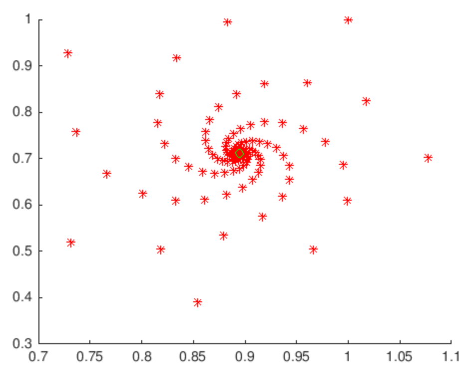
(a)

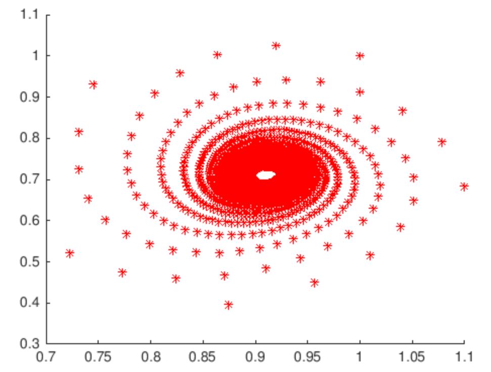
(b)

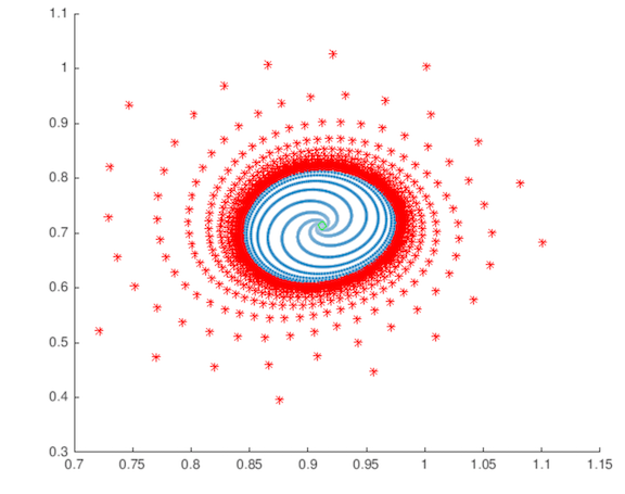
(c)

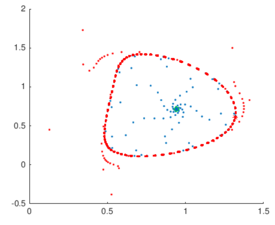
(d)

Figure 9: Poincaré sections: attracting fixed point. (Top left) attracting fixed point in the Poincare section for $\alpha=0.65$. (Top right) Neimark-Sacker bifurcation for $\alpha=\alpha_{1}$. (Bottom left) repelling fixed point of the Poincaré map and attracting invariant circle for $\alpha=0.7$. (Bottom right) repelling fixed point and attracting invariant circle for $\alpha=0.8$. In the bottom frames, blue points represent orbits diverging from the repelling fixed point and converging to the attracting invariant circle from inside. In all frames red points represent orbits converging to the attractor from the outside. This circle itself is located by iterating the Poincaré map sufficiently long.

Figure 10: Schematic of a resonant torus: the green dot is a stable cycle and the red dot a saddle cycle. Black curves are stable/unstable manifolds. The unstable manifold of the saddle cycle accumulates at the stable cycle, forming an invariant topological circle. The smoothness of the circle depends on the eigenvalues at the stable cycle, and if the eigenvalues at the stable cycle are complex conjugate the circle cannot be globally differentiable.

3.2 Resonant tori

When $\alpha>0$ is large enough the dynamics on the invariant circle $\Gamma$ change in a fundamental way, as we now discuss. We say that $q$ is a period $k$ point for $R\colon\mathbb{R}^{2}\to\mathbb{R}^{2}$ if $q,R(q),R^{2}(q),\ldots,R^{k-1}(q)$ is a collection of $k$ distinct points having $R^{k}(q)=q$. We say that the point set

$$\mathcal{Q}=\mbox{orbit}(q)=q\cup R(q)\cup R^{2}(q)\cup\ldots\cup R^{k-1}(q)\subset\mathbb{R}^{2},$$

is a $k$-cycle for $R$. Notions like stability and stable/unstable manifolds of $k$-cycles are defined in the obvious way after observing that $q$ and each of its iterates are fixed points of the composition map $R^{k}$. See for example [50] for precise definitions and references to the literature. The following notion is critical in the discussion to follow.

Definition 3.1.

Let $R\colon\mathbb{R}^{2}\to\mathbb{R}^{2}$ be a smooth map of the plane and $\Gamma\subset\mathbb{R}^{2}$ be a topological circle invariant under $R$. We say that $\Gamma$ is a simple resonant invariant circle if there is an attracting $k$-cycle $\mathcal{Q}_{1}$ and a saddle $k$-cycle $\mathcal{Q}_{2}$ so that

$$\Gamma=\{\mathcal{Q}_{1}\}\cup\{\mathcal{Q}_{2}\}\cup W^{u}(\mathcal{Q}_{2}).$$

The situation is that the one dimensional unstable manifold of the saddle cycle is completely absorbed into the basin of attraction of the stable cycle, in such a way that a circle is formed. In this case the dynamics on the invariant circle are conjugate to a gradient system. Observe that the unstable manifold of the saddle cycle is smooth (analytic if the map is), even if – as we will see below – the regularity of the invariant circle is another matter completly. The situation is illustrated in Figure 10 for the simple case of a one-cycle.

Remark 3.2.

If the decomposition of $\Gamma$ requires multiple stable and saddle cycles of different periods we say that we have a compound resonant invariant circle. However we do not encounter this situation in the present study, and for this reason we usually drop the term “simple” and say simply that we have a resonant invariant circle.

Remark 3.3.

Suppose that $R$ is a Poincaré map for a 3-dimensional smooth vector field $f$, and that $R$ has a simple resonant invariant circle $\Gamma$. Then the flow generated by $f$ has a resonant invariant torus given by

$$\mathcal{T}\mathrel{\mathop{\mathchar 58\relax}}=\left\{\phi_{t}(v)\mathrel{\mathop{\mathchar 58\relax}}v\in\Gamma,t\in\mathbb{R}\right\}.$$

We further remark that the global regularity of a resonant invariant circle (or torus) is determined by the linearization of $R$ at $q_{1}$ or any of its iterates. So for example if $DR(q_{1})$ has real distinct stable eigenvalues then the resulting invariant circle is finitely differentiable, with regularity determined by the ratio of these eigenvalues. If on the other hand $DR(q_{1})$ has complex conjugate eigenvalues then the torus in phase space is only $C^{0}$, as the unstable manifold of $\mathcal{Q}_{2}$ is forced to approach $\mathcal{Q}_{1}$ in a spiraling fashion and the resulting curve cannot be differentiable or even Lipschitz at $q_{1}$ or any of its iterates.

3.3 Resonant tori in the Langford system

The formation of a resonant invariant torus in the Langford system of Equation (1) involves a global bifurcation which can be observed in the Poincaré section, as we now describe. We begin with the observation that at $\alpha=0.82$ there is an attracting $3$-cycle, which we denote by $\mathcal{Q}_{1}$, and which lies outside the invariant circle $\Gamma$. The basin of attraction of the $3$-cycle is fairly small, as there is a saddle type $3$-cycle nearby, which we denote by $\mathcal{Q}_{2}$.

For parameter values near $\alpha=0.82$, the unstable manifold of $\mathcal{Q}_{2}$ has the following behavior: half of $W^{u}(\mathcal{Q}_{2})$ accumulates on the attracting invariant circle $\Gamma$ while the other half accumulates to the attracting $3$-cycle $\mathcal{Q}_{1}$. Things remain much the same for nearby parameter values, for example at $\alpha=0.8224$, with the caveat that the saddle $3$-cycle $\mathcal{Q}_{2}$ has moved closer to $\Gamma$. The situation is illustrated in Figure 11. The stable manifold of $\mathcal{Q}_{2}$ appears to form a separatrix between the basins of attraction of $\Gamma$ and $\mathcal{Q}_{1}$. See for example the left frame of Figure 11.

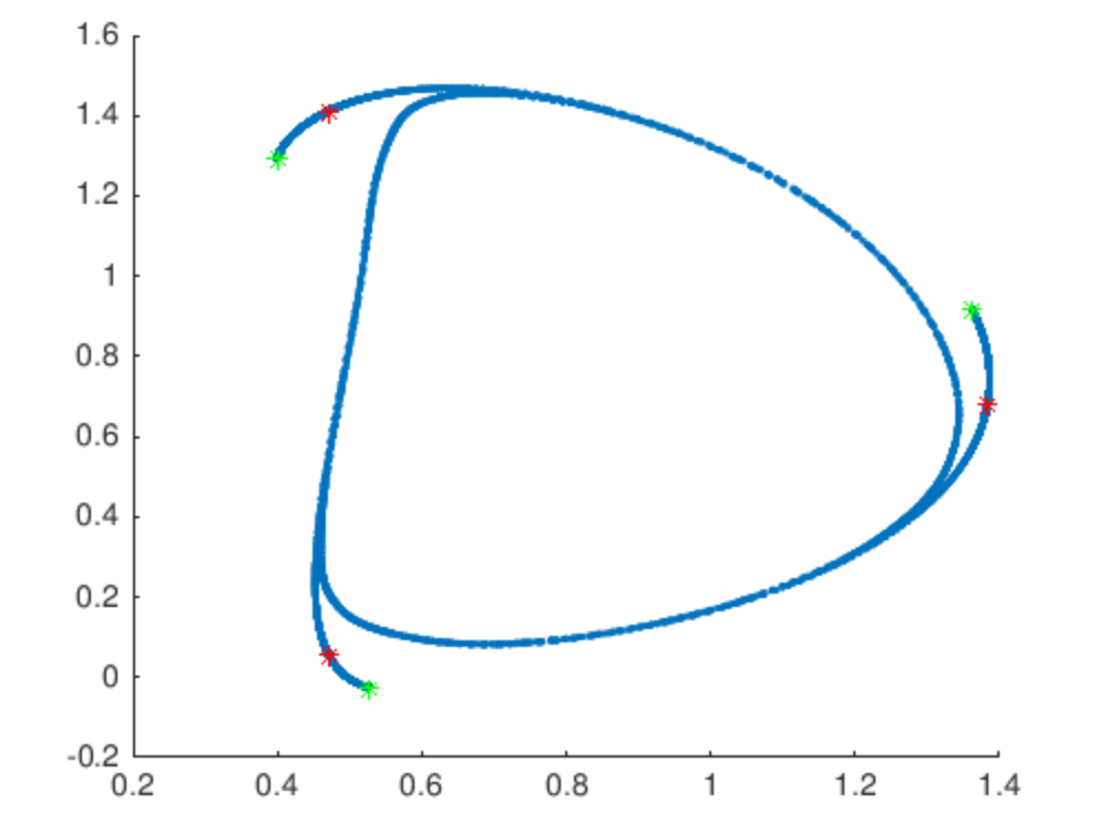
(a)

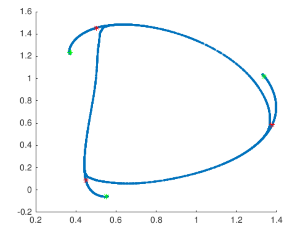
(b)

Figure 11: Unstable manifold of the saddle $3$-cycle accumulating to both the invariant circle and the stable $3$-cycle: The three red dots illustrate the saddle $3$-cycle $\mathcal{Q}_{2}$ while the three green points illustrate the attracting $3$-cycle $\mathcal{Q}_{1}$. The blue curve represents the unstable manifold of $\mathcal{Q}_{2}$. In both cases half the unstable manifold accumulates on $\Gamma$, and half accumulates on $\mathcal{Q}_{1}$. In the left frame $(\alpha=0.82)$ the saddle is far from the invariant circle but in the right frame $(\alpha=0.8224)$ it has moved much closer in anticipation of the coming global bifurcation.

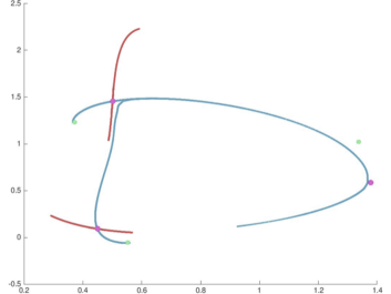
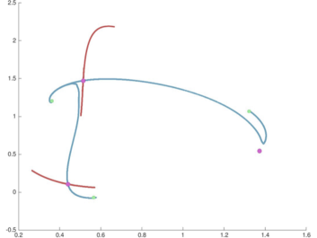
Figure 12: The resonant torus: before and after. $W^{s}(\mathcal{Q}_{2})$ is red and $W^{u}(\mathcal{Q}_{2})$ is blue. The stable cycle is marked with three green points and the saddle cycle marked by magenta. (Left) at $\alpha=0.822$ note the top left magenta point. The left side of its unstable manifold goes to the attracting orbit (green point) while its right side wraps around the attracting invariant circle. (Right) at $\alpha=0.826$ the bifurcation has occurred and the invariant circle is resonant, now comprised of the two $3$-cycles and the unstable manifold. Looking again at the top left magenta point, the left side of $W^{u}(\mathcal{Q}_{2})$ still accumulates to the top left green point in the attracting orbit, the right side now loops back and is “captured” by the top right green point. Hence both sides of the unstable manifold now accumulate to the attracting cycle.

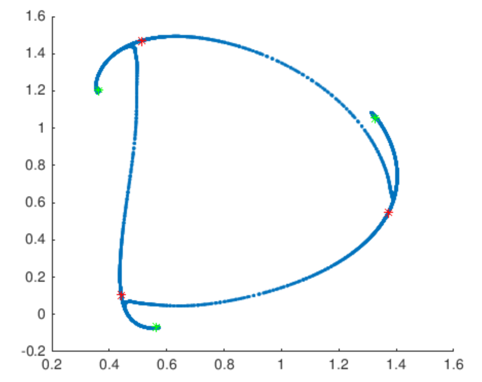
(a)

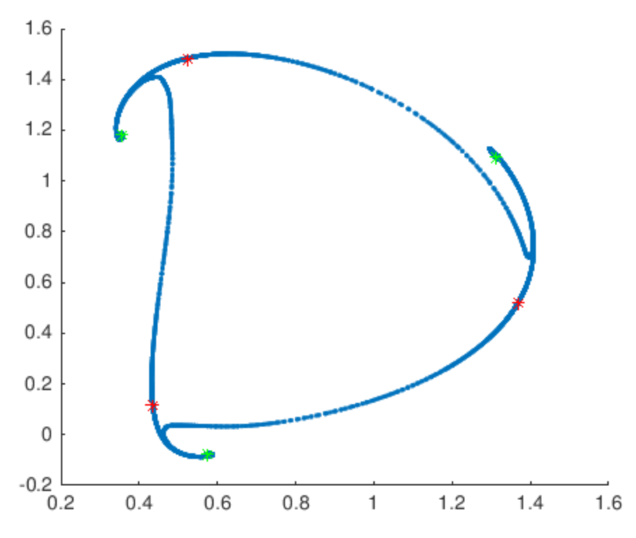
(b)

Figure 13: Resonant invariant circles in the Poincaré section. Colors have the same meaning as in Figure 11. (Left) at $\alpha=0.825$ the saddle $3$-cycle has collided with the invariant circle. (Right) a larger value of $\alpha=0.83$, the resonant invariant circle $\Gamma$ is becoming less regular and lacking differentiability.

For some parameter value $0.8224<\alpha_{2}<0.825$ there appears to be a global bifurcation where $\mathcal{Q}_{2}$ collides with the invariant circle $\Gamma$. At this point $W^{u}(\mathcal{Q}_{2})$, rather than accumulating on the invariant circle $\Gamma$, has become $\Gamma$. Both halves of the unstable manifold accumulate at $\mathcal{Q}_{1}$, which is now inside the invariant circle as well. See Figure 12 for an illustration of the phase space configuration just before and just after the global bifurcation. The situation remains for parameter values $\alpha>\alpha_{2}$ as illustrated in Figure 13.

Let $q_{1}$ and $q_{2}$ be points on the $3$ cycles $\mathcal{Q}_{1}$ and $\mathcal{Q}_{2}$ respectively. By numerical calculation we find that the eigenvalues of $DR^{3}(q_{1})$ are complex conjugate stable. Then the resonant invariant circle appearing in this bifurcation is only $C^{0}$. This is a dramatic change, as for $\alpha<\alpha_{2}$ the simulations indicate that the torus is smooth (at least finitely differentiable). The global bifurcation just described gives a vivid natural example of a low regularity invariant manifold for a smooth (in fact analytic) vector field.

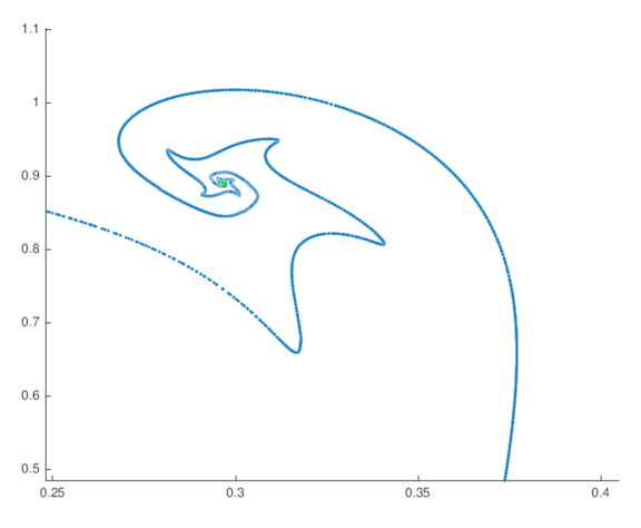
(a)

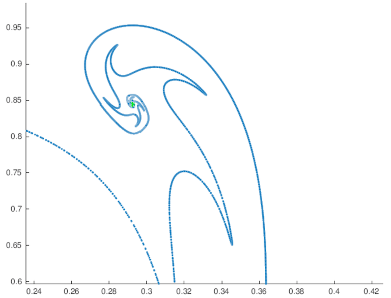
(b)

(c)

Figure 14: Resonant torus near the attracting $3$-cycle: Closeups on an attracting period $3$ point for three different values of $\alpha$ larger than $\alpha_{2}$. It is clear that the invariant circle is becoming increasingly irregular, developing sharp cusp-like edges in its embedding.

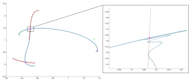
Figure 15: Transient chaos: At $\alpha=0.8225$ there are transverse intersections of $W^{u}(\mathcal{Q}_{2})$ and $W^{s}(\mathcal{Q}_{2})$ indicating the presence of Smale horseshoes and thus chaotic dynamics near the attracting resonant invariant torus $\mathcal{T}$ in phase space. Note that, in contrast, the dynamics on the attractor are very simple – that is, the chaos is transient. This image tells us that, since $W^{u}(\mathcal{Q}_{2})$ and $W^{s}(\mathcal{Q}_{2})$ do not intersect at $\alpha=0.8224$ (see Figure 12), the global bifurcation to a resonant torus occurs for $0.8224<\alpha_{2}<0.8225$.

3.4 Transient chaotic motions

Increasing the bifurcation parameter $\alpha$ past the global bifurcation at $\alpha_{2}$ shows that the embedding of the attracting $C^{0}$ resonant invariant circle $\Gamma$ appears to get even “wilder”. See the three frames of Figure 14. The blue curve illustrates the unstable manifold of $\mathcal{Q}_{2}$ and in the left two frames is contained in the invariant circle $\Gamma$, indicating that the circle is loosing regularity.

A more quantitative discussion about dynamical complexity in the system begins by observing that just before the global bifurcation at $\alpha_{2}$, as $\mathcal{Q}_{2}$ is approaching $\Gamma$, there is the appearance of chaotic dynamics in the system. To see this we observe that in the top left corner of the left hand frame of Figure 12, the unstable manifold of $\mathcal{Q}_{2}$ (vertical blue curve) is to the right side of the stable manifold (vertical red curve). In the top left corner of the right hand frame in the same figure we see that the situation is reversed: the unstable manifold now being to the left of the stable one (again vertical blue and red respectively). Since the curves move continuously this suggest that there should be a range of parameters where they intersect.

Figure 15 shows that this is indeed the case. At $\alpha=0.8225$ we can see that the resonant torus in phase space has not formed yet, as the unstable manifold (blue curve) does not accumulate at the stable $3$-cycle (green point). Here, on close inspection we see that $W^{s}(\mathcal{Q}_{2})$ and $W^{u}(\mathcal{Q}_{2})$ do intersect, in fact transversally. Then there is a Smale horse shoe and hence chaotic dynamics in a neighborhood of $\Gamma$ [78]. Note however that the invariant circle $\Gamma$ is still attracting and that the dynamics on $\Gamma$ are simple before and after the global bifurcation at $\alpha_{2}$. This suggests that the chaotic motions are only transient, in the sense that the horse shoe is not in the attractor.

3.5 Destruction of the torus and appearance of a chaotic attractor

By further increasing the bifurcation parameter we eventually observe the destruction of the invariant torus, as we now describe. We begin by recalling a classical result concerning the disappearance of an invariant circle. We refer to the discussion in [36] for the details of the proof and generalizations to higher dimensions. See also [79] and [5, 15, 16]. The set up is as follows.

Suppose that a one parameter family of smooth discrete time dynamical systems $R_{\alpha}\colon\mathbb{R}^{2}\to\mathbb{R}^{2}$ has at $\alpha=\alpha_{0}$ a resonant $C^{0}$ invariant circle $\Gamma\subset\mathbb{R}^{2}$ formed by the closure of the unstable manifold of a saddle cycle $\mathcal{Q}_{2}$ accumulating to a stable cycle $\mathcal{Q}_{1}$ as in Figure 10. We then have a resonance region in the sense of [36] and, while it may be obvious it is nevertheless important to note that, the resonant torus $\Gamma$ is robust under small perturbations including small changes in $\alpha$. This is because the saddle cycle, the attracting cycle, and any local unstable manifold of the saddle are structurally stable objects. Since a local unstable manifold is all that is required to reach the basin of attraction of $\mathcal{Q}_{1}$, we have that the resonant torus is robust. It follows that there is a one parameter family of attracting invariant circles $\Gamma(\alpha)$ for $\alpha$ near $\alpha_{0}$. Indeed the tori vary continuously in $\alpha$, again see [36].

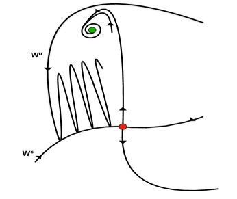
(a)

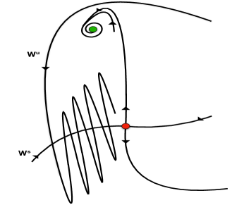
(b)

Figure 16: Schematic of the tangency: one mechanism for the destruction of a $C^{0}$ resonant invariant circle (see Figure 10) is the formation of a homoclinic tangency (we stress that many tangencies may appear at the same time [74]). Suppose that before the tangency $W^{u}$ of the saddle cycle is absorbed into the basin of attraction of a stable cycle (green point). Once a tangency forms $W^{u}$ of the saddle cycle must also accumulate in a $C^{1}$ fashion on $W_{\mbox{{\tiny loc}}}^{u}$ near the saddle (red point) – while still accumulating at the stable cycle – and the resonant torus is destroyed. The bifurcation is discussed in greater detail in [36].

Now, suppose that at some parameter $\hat{\alpha}>\alpha_{0}$ the invariant torus no longer exists. Then, by the least upper bound property of $\mathbb{R}$ there is an $\alpha^{*}$ so that $\Gamma$ is a continuous attracting invariant circle on the interval $[\alpha_{0},\alpha^{*})$, but that for $\alpha>\alpha^{*}$ this fails to be true. The theorem on torus breakdown [36] asserts the following three possible mechanisms for the destruction of $\Gamma$: (i) loss of cycle stability– i.e. a local bifurcation at $\mathcal{Q}_{1}$, (ii) occurrence of a tangency bifurcation of the stable and saddle cycles on $\Gamma$, or (iii) formation of a homoclinic tangency between $W^{u}(\mathcal{Q}_{2})$ and $W^{s}(\mathcal{Q}_{2})$. Mechanism (iii) is illustrated schematically in Figure 17.

Of course the theorem gives only a trichotomy. It does not say which alternative actually occurs in a given example, and it is with this in mind that we investigate the fate of the invariant torus in the Langford system. The situation is illustrated in the two frames of Figure 17, where we observe the formation of a homoclinic tangle for $W^{u,s}(\mathcal{Q}_{2})$. Since these manifolds do not intersect in the frame on the left, and do intersect in the frame on the right, they must develop a tangency at some point $0.92<\alpha_{3}<0.93$. While the closure of the unstable manifold (blue) on the left is still an attracting invariant circle, in the right frame $W^{u}(\mathcal{Q}_{2})$ is no longer contained in the attractor suggesting that the torus was destroyed in the homoclinic tangency – that is that we have in alternative (iii).

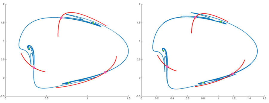
(a)

Figure 17: Global bifurcation and destruction of the invariant circle: (Left) for $\alpha=0.92$ the unstable manifold of $\mathcal{Q}_{2}$ (blue) still accumulates (albeit in a complicated way) to the stable three cycle $\mathcal{Q}_{1}$, and the attractor is still a resonant invariant circle. That being said, we can see sharp turns developing in the embedding of the unstable manifold near the stable manifold (red curve) of $\mathcal{Q}_{2}$. (Right) at $\alpha=0.93$, these sharp turns in the unstable manifold embedding have moved across the stable manifold resulting in points of transverse intersection and hence a Smale horse shoe nearby.

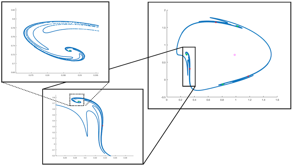
(a)

Figure 18: Fractal structure of $W^{u}(\mathcal{Q}_{2})$: at $\alpha=0.9321$, after the formation of the homoclinic tangency, the structure of the unstable manifold is much more complicated.

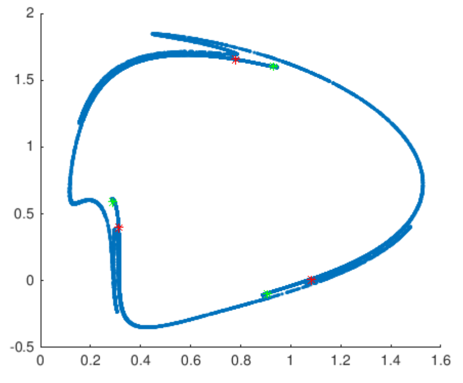
(a)

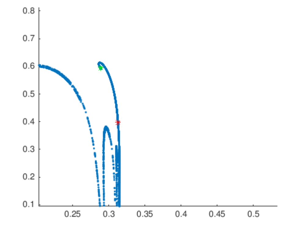
(b)

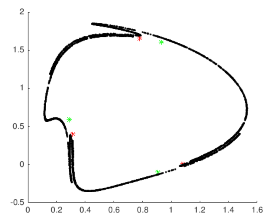
(c)

Figure 19: All three figures were plotted using $\alpha=0.95$. (Left) unstable manifold of the saddle period three cycle in the Poincaré section, colors have the same meaning as in Figure 11. (Center) the fractal structure of $W^{u}(\mathcal{Q}_{2})$ is no longer present going into the stable cycle. (Right) the torus $\mathcal{T}$ in phase space is destroyed and trajectories fall in a set with fractal dimension $2+d$, $d<1$. Both period three cycles have moved inside the invariant set (black).

Further numerical evidence for this claim is given in the three frames of Figure 19. Here the bifurcation parameter is increased slightly further to $\alpha=0.95$ so that the picture opens up a little. The frame on the right is obtained by iterating a large number of initial conditions until they numerically converge to the attractor, represented by the black curve. Note that the stable and saddle $3$-cycles (green and red collections of dots) appear to have moved off the attractor as they do not touch the black curve. This indicates multi-stability in the system as the green orbit is itself attracting. Moreover the left frame shows the numerically computed unstable manifold $W^{u}(\mathcal{Q}_{2})$, and it is clear by comparing the left with the right frame that – while $W^{u}(\mathcal{Q}_{2})$ is accumulating on the chaotic attractor union $\mathcal{Q}_{1}$, the unstable manifold of $\mathcal{Q}_{2}$ is no longer contained in the attractor. This becomes even more clear when we look again at the right frame of the figure and see no black line from the red dots to the green: hence the attractor is no longer a resonant torus.

Zooming in suggests in fact that the attractor is now a quite complicated shape, as illustrated in the middle frame of Figure 19, and also in Figure 18. Indeed Figure 18 reveals the fractal structure of the unstable manifold of $\mathcal{Q}_{2}$. The actual structure of the set is even more complicated than any picture can reveal, as results from topological dynamics imply that once there is a transverse homoclinic for $\mathcal{Q}_{2}$ the closure of the unstable manifold, which contains the attractor, is an indecomposable continuum [80, 81]. We refer also the the work of [82] on the persistence of normally hyperbolic invariant manifolds in the absence of uniform rates and to the much more recent and constructive work of [83].

3.6 Visualizing the torus in phase space

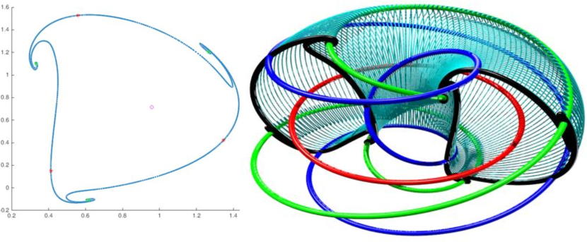
Figure 20: Cut-away at $\alpha=0.85$: The left frame recalls the invariant set in the Poincaré section when $\alpha=0.85$, which is a resonant invariant circle formed by two period three cycles. The right frame illustrates the corresponding invariant set in phase space. The red curve is the repelling periodic orbit $\gamma$ which originally underwent the Neimark-Sacker bifurcation. The green curve is the attracting periodic orbit $\gamma_{1}$ corresponding to the attracting period three cycle, while the blue curve is the saddle periodic orbit $\gamma_{2}$ corresponding to the saddle $3$-cycle in the Poincaré section. The half torus (colored in teal) is obtained by advecting the section’s invariant circle $\Gamma$ under the flow. Since the invariant circle is formed by the unstable manifold of the saddle cycle, the teal surface represents $W^{u}(\gamma_{2})$. The resulting invariant set is a topological, but not smooth, invariant attracting resonant torus.

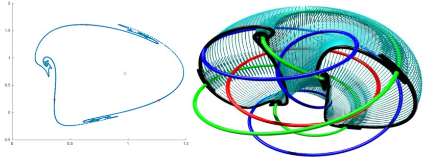
Figure 21: Cut-away at $\alpha=0.9$: same color scheme as in Figure 20. Complicated embedding of the attracting resonant invariant torus.

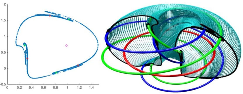
Figure 22: Cut-away at $\alpha=0.929$: same color scheme as in Figure 20. The unstable manifold of the saddle type period three cycle in the Poincaré section side-by-side with the unstable manifold of $\gamma_{2}$ in phase space, just after the global bifurcation triggered by the homoclinic tangency at $\alpha_{3}$. The unstable manifold accumulates on the union of the stable periodic orbit $\gamma_{1}$ and the chaotic attractor.

Studying the dynamics of a three dimensional system in a two dimensional Poincaré section helps us to locate bifurcations of the invariant tori by reducing them to invariant circles. Nevertheless, it is still desirable to visualize dynamical structures of the original system in the full phase space, and to this end we provide several images which show side by side the invariant objects found in the Poincaré section and the corresponding invariant objects for the full Langford system.

See for example Figure 20. The left frame illustrates the attracting invariant circle in the section for the parameter value $\alpha=0.85$. The three red and green dots represent the saddle type and stable $3$-cycles $\mathcal{Q}_{2}$ and $\mathcal{Q}_{1}$ respectively. The magenta dot in the center of the frame represents the repelling fixed point, while the blue curve is the unstable manifold of the saddle. The blue curve is clearly absorbed into the basin of attraction of the stable $3$-cycle, forming a resonant invariant circle. The $3$-cycles $\mathcal{Q}_{1},\mathcal{Q}_{2}$ give rise to periodic solutions in $\mathbb{R}^{3}$, which we denote by $\gamma_{1}$ and $\gamma_{2}$ respectively.

The right frame of the same figure illustrates the embedding in phase space of the same objects. Here the red curve represents the repelling periodic orbit $\gamma$, green curve the attracting periodic orbit $\gamma_{1}$, and the blue curve is the saddle periodic orbit $\gamma_{2}$. The unstable manifold of $\gamma_{2}$ accumulates at $\gamma_{1}$ forming the resonant torus. Half of the torus is cut-away so that the skeleton given by the periodic orbits stands our clearly.

Figures 21 and 22 depict the same information at $\alpha=0.9$ and $\alpha=0.929$. Taken together the three images provide much more insight into the structure of the invariant dynamics than can be gained by studying simulations of individual orbits like those illustrated in Figure 3.

4 Global dynamics

We now come to the second part of the present work, and study the dynamics not on but near the attracting invariant torus. The remaining important features of the surrounding phase space are the equilibrium solutions on the $z-$ axis, and their invariant manifolds. For this part of the study we abandon the Poincaré section and consider features of the three dimensional phase space.

4.1 Accumulation of $W^{u}(p_{0})$ on a component of the global attractor

One of the most important features in the phase space of the Langford system is the equilibrium point $p_{0}\in\mathbb{R}^{3}$, which for all $\alpha\geq 0$ is located on the positive $z$ axis and which has two dimensional unstable manifold and one dimensional stable manifold. For all $\alpha\geq 0$ the stable manifold of $p_{0}$ is a subset of the $z$-axis. The two dimensional unstable manifold on the other hand is much more interesting. All the calculations in this section are preformed using the parameterization method/continuation scheme as discussed in the Section 2.

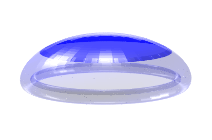
(a) $\alpha=0$

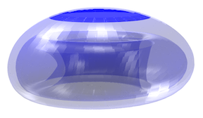
(b) $\alpha=0.6$

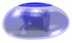
(c) $\alpha=0.7$

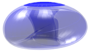
(d) $\alpha=0.8$

(e) $\alpha=0.806$

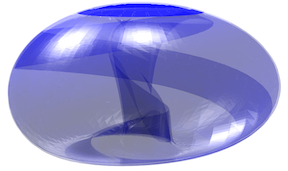
(f) $\alpha=0.9321$

Figure 23: Unstable manifold “bubble” for the saddle $p_{0}$: for the indicated values of $\alpha$. The computations suggest the existence of a periodic orbit which undergoes a Neimark-Sacker bifurcation. The phase space is then dominated by the resulting smooth invariant torus. The computations for higher $\alpha$ suggest that the smoothness of the torus may breakdown as $\alpha$ increases.

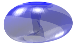
(a) $\alpha=0.95$

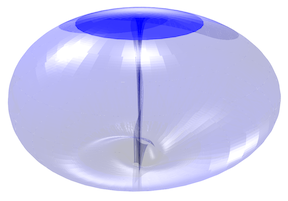
(b) $\alpha=1.1022$

Figure 24: Unstable manifold of $p_{0}$ after the saddle node bifurcation: (Left) $\alpha=0.95$. The bubble develops a “stripe” which is due to the manifold folding over itself as it accumulates on the union of the chaotic attractor and the attracting periodic orbit. (Right) $\alpha=1.1022$, the quality of the bubble has changed dramatically. It is more “open” and appears to accumulate on the $z$-axis.

Recall that for $0\leq\alpha\leq\alpha_{4}\approx 0.9321697517861$, the point $p_{0}$ is the only equilibrium of the Langford system. The manifold $W^{u}(p_{0})$ is illustrated in Figure 23 for six such values of $\alpha$. We see that for $\alpha<\alpha_{1}$ – the value of the Neimark- Sacker bifurcation – $W^{u}(p_{0})$ accumulates on the attracting periodic orbit $\gamma$ as seen in frame (a) of Figure 23. The periodic orbit $\gamma$ appears to be the global attractor in this parameter range.

After the Neimark- Sacker bifurcation at $\alpha_{1}\approx 0.697144898322973$ the periodic orbit $\gamma$ is repelling and $W^{u}(p_{0})$ appears to accumulate on the smooth attracting invariant torus $\mathcal{T}$ which was discussed at length in Section 3. This is seen in frames (b), (c) and (d) of Figure 23. Frames (d) and (e) illustrate the situation after the appearance of the attracting period three cycle in the Poincaré section (see Figure 11), and there is an attracting periodic orbit in phase space which we denote by $\gamma_{1}$. The system is bistable, with the attractor being the union of the invariant torus $\mathcal{T}$ and the periodic orbit $\gamma_{1}$. The manifold $W^{u}(p_{0})$ accumulates on the union of these two objects – a disjoint set – and this is what introduces the rough folds in the embedding seen in Frames (d) and (e).

Frame (f) illustrates the embedding of $W^{u}(p_{0})$ for $\alpha>\alpha_{2}$ but just before the global bifurcation at $\alpha=\alpha_{4}$ which destroys the torus. Here the torus is resonant and only $C^{0}$, a fact which is clearly reflected in the embedding of $W^{u}(p_{0})$.

For $\alpha>\alpha_{4}$ we are past the saddle node bifurcation, and $p_{0}$ is no longer the unique equilibrium. This has dramatic consequences for the global dynamics, and we illustrate the unstable manifold for two such parameter values in Figure 24. Somewhere between $\alpha=0.95$ (frame (a) of the figure) and $\alpha=1.1022$ (frame (b)) something dramatic happens. The change however is not easily understood by looking only at $W^{u}(p_{0})$, and we must consider the embedding of new invariant objects which appear only after the occurrence of the saddle node bifurcation.

4.2 $W^{s}(p_{1})$ as a separatrix

At $\alpha_{4}\approx 0.9321697517861$ the system undergoes a saddle node bifurcation, resulting in the appearance of two new equilibrium solutions denoted $p_{1}$ and $p_{2}$. For all $\alpha>\alpha_{4}$ the point $p_{2}$ is a stable equilibrium, making $p_{2}$ a new component of the global attractor. The equilibrium solution at $p_{1}$ on the other hand is a saddle, with one dimensional unstable manifold on the $z$-axis and a two dimensional stable manifold associated with a pair of complex conjugate eigenvalues.

Our simulations suggest that for some range of $\alpha>\alpha_{4}$, the two dimensional invariant manifold $W^{s}(p_{1})$ is a separatrix for the basin of attraction of $p_{2}$ and the attractor onto which $W^{u}(p_{0})$ accumulates. In this sense, $W^{s}(p_{1})$ forms a kind of “bubble”, where inside the bubble we have an attractor comprised of either the resonant torus $\mathcal{T}$ or the chaotic set which appears after the destruction of $\mathcal{T}$. The inside of the bubble is the basin of attraction of this attractor, and the outside of the bubble is the basin of the stable equilibrium $p_{2}$. The situation is illustrated in Figure 25.

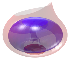
(a)

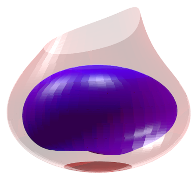
(b)

Figure 25: 2D stable and unstable manifolds of equilibria of $p_{0}$ and $p_{1}$:. At $\alpha=0.95$ we note that $W^{u}(p_{0})$ (blue) and $W^{s}(p_{1})$ (red) do not intersect at all. We also remark that $p_{2}$ (not shown) is below $p_{1}$ and is an attracting equilibrium point. The attracting torus (or “torus-like” chaotic attractor) is inside the “bubble” formed by these stable/unstable manifolds.

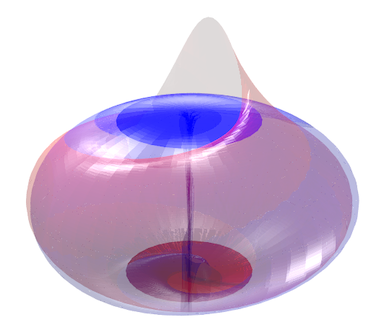
(a)

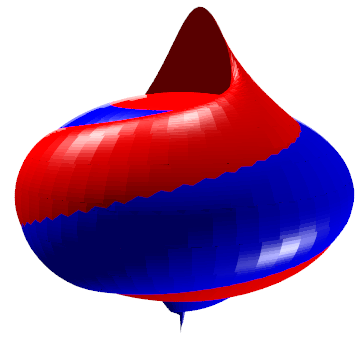
(b)

Figure 26: 2D stable and unstable manifolds of equilibria of $p_{0}$ and $p_{1}$ for $\alpha=1.1022$. Here we see that $W^{u}(p_{0})$ (blue) and $W^{s}(p_{1})$ (red) appear to intersect transversely. The intersection curves are then heteroclinic orbits from $p_{0}$ to $p_{1}$. The unstable manifold accumulates on the $z$-axis, as seen in the transparency on the left. The frame on the right suggests that the unstable manifold enters the basin of attraction of $p_{2}$. In fact, for $\alpha=1.1022$ it seems that $p_{2}$ is the unique attractor.

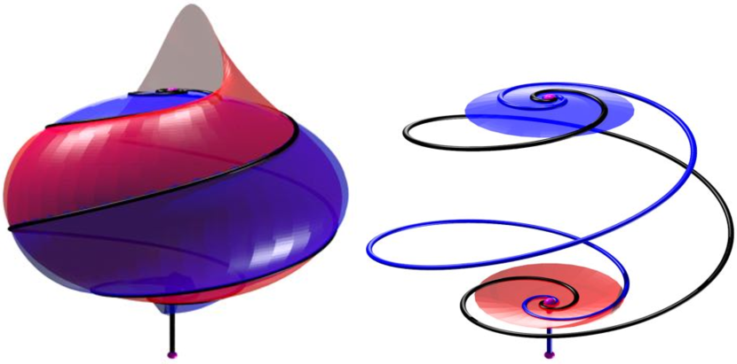
Figure 27: Heteroclinic connections from $p_{0}$ to $p_{1}$ for $\alpha=1.1022$. Encouraged by the apparent transverse intersections seen in Figure 26, we locate heteroclinic orbit segments starting on $W^{u}(p_{0})$ and terminating on $W^{s}(p_{1})$ by applying a Newton scheme to the boundary value problem describing the segments. Observe that the heteroclinic orbit segments located are much smoother than the apparent intersection seen in Figure 26. The apparent irregularity of the intersection is due to the fact that we compute piecewise linear triangulations of the fundamental domain and its iterates.

4.3 Heteroclinic intersections and the loss of bistability

Studying $W^{u}(p_{0})$ and $W^{s}(p_{1})$ reveals yet another global bifurcation which dramatically alters the phase space dynamics of the system. It appears that for some $\alpha_{5}\approx 1.05$ these manifolds develop a tangency, and that after this tangency there are transverse heteroclinic connections from $p_{0}$ to $p_{1}$. The situation is illustrated in Figures 26 and 27, where we see the transverse intersections of the manifolds and the resulting heteroclinic connections respectively.

Once intersections appear between $W^{u}(p_{0})$ and $W^{s}(p_{1})$, the latter ceases to function as a separatrix, and orbits can pass from inside the bubble to outside. The equilibrium $p_{2}$ remains attracting and its basin appears now to extend into the inside of the bubble. Indeed our numerical simulations suggest that for $\alpha>1$, that is after the formation of intersections between the unstable/stable manifolds of $p_{0}$ and $p_{1}$, the equilibrium $p_{2}$ becomes the global attractor for the system. That is, all orbits which start inside the bubble eventually accumulate there. This finally explains the “openness” of Figure 24 (b) remarked upon earlier: the occurrence of the heteroclinic tangency between $W^{u}(p_{0})$ and $W^{s}(p_{1})$ appears to destroy the attractor which had previously dominated the dynamics inside the bubble.

5 Conclusions and Discussion

We will summarize the results of the present work by sketching the main features of the global dynamics of the Langford system (1) as suggested by our analysis. First recall the main local and global bifurcations undergone by the system.

• At $\alpha_{1}\approx 0.697144898322973$ the periodic orbit $\gamma$ undergoes a Neimark-Sacker bifurcation. This is a local bifurcation of $\gamma$ which results in the appearance of the invariant torus $\mathcal{T}$.

• At $\alpha_{2}\approx 0.823$ the invariant torus $\mathcal{T}$ develops a resonance. After this $\mathcal{T}$ is the union of two periodic orbits $\gamma_{2}$ (saddle stability), and $\gamma_{1}$ (attracting), and the unstable manifold of $\gamma_{2}$. The resonance is triggered by the collision of a saddle periodic orbit with the invariant torus. Since the torus is an attractor before and after the collision, this bifurcation involves no change in the stability of $\mathcal{T}$ and is hence a global bifurcation.

• At $\alpha_{3}\approx 0.925$ there is a global bifurcation triggered by the formation of a tangency between $W^{s}(\gamma_{1})$ and $W^{u}(\gamma_{1})$.

• At $\alpha_{4}\approx 0.9321697517861$ there is a saddle node bifurcation resulting in the appearance of the equilibrium points $p_{1}$ (saddle-focus stability) and $p_{2}$ (attracting). This is a local fold bifurcation for the equilibrium points.

• At $\alpha_{5}\approx 1$ a global bifurcation is triggered by the development of a tangency between $W^{u}(p_{0})$ and $W^{s}(p_{1})$.

Between the bifurcation values listed above, we conjecture based on our numerical studies that the system has the following properties.

Conjecture 5.1 (Sketch of the global dynamics).

The flow generated by the Langford vector field, given in Equation (1), has that;

1. For $0<\alpha<\alpha_{1}$ the periodic orbit $\gamma$ is the global attractor.

2. For $\alpha_{1}<\alpha<\alpha_{2}$ the global attractor is either $\mathcal{T}$ or $\mathcal{T}\cup\gamma_{1}$.

3. For $\alpha_{2}<\alpha<\alpha_{3}$ the global attractor is $\mathcal{T}$.

4. For $\alpha_{3}<\alpha<\alpha_{4}$ the global attractor is $\mathcal{T}\cup p_{2}$.

5. For $\alpha_{4}<\alpha<\alpha_{5}$ there is multi-stability. The global attractor is comprised of at least the components $\tilde{\mathcal{T}}$ - the chaotic attractor appearing after the break-up of the invariant torus, the attracting periodic orbit $\gamma_{2}$, and the attracting equilibrium solution $p_{2}$.

6. For $\alpha>\alpha_{5}$ the equilibrium solution $p_{2}$ is the global attractor.

7. For $0<\alpha<\alpha_{3}$ the unstable manifold $W^{u}(p_{0})$ accumulates on the global attractor, which is either $\gamma$ (until $\alpha=\alpha_{1}$) or $\mathcal{T}$.

8. For $\alpha_{3}<\alpha<\alpha_{5}$ the stable manifold $W^{s}(p_{1})$ is a separatrix. The basin of attraction of $p_{2}$ is outside the bubble formed by $W^{s}(p_{1})$.

It is essential to stress that the eight points above are still just conjectures, however well informed. The numerical work carried out in the present work is not sufficient to rule out other components of the global attractor, for example other attracting periodic orbits near the resonant torus or the chaotic attractor. This point is elaborated on below.

It is also worth remarking that softer sorts of conclusions are encapsulated in the paper’s many figures. The deliberate calculations and three dimensional renderings of invariant manifolds throughout our work provide more delicate insights into the dynamics of the system than are obtained by straight forward simulations of ensembles of initial conditions. As a final illustration of this point we give in Figure 28 a side by side comparison of the results obtained using the methodology of the present work with the results obtained by direct integration, for the parameter value $\alpha=0.9321$. Simulation results cannot illuminate the full attractor, as numerical integrations will never reveal the unstable periodic orbit $\gamma_{2}$ which lies inside the invariant torus $\Gamma$.

More generally, since the Langford system is derived by truncating the normal form of a cusp-Hopf singularity, we expect qualitatively similar behavior in systems exhibiting this bifurcation. An interesting topic for future research would be to repeat the numerical analysis performed in the present work for other modifications of the normal form. For example one could perturb the system in such a way that the $z$-axis is no longer invariant. Or, one could modify the system so that the Neimark-Sacker bfurcation is subcritical rather than supercritical.

As remarked already in [20] (and in the introduction of the present work) complex dynamics are often generated by interactions between equilibrium and periodic solutions. The fact that the Langford system is close to a simultaneous cusp-Hopf bifurcation is precisely what provides the multiple equilibrium solutions in close proximity to a limit cycle. This is the basic mechanism organizing many of the interesting dynamical phenomena discussed in the present work.

The normal form unfolding a pitchfork-Hopf bifurcation was also studied by Langford in [84], and it would be a nice project to apply the methods of the present work to this system, or to systems derived from the fold-Hopf bifurcation. Other important normal forms are discussed for example in the woks of [85, 86, 87].

Another interesting topic of future work would be to prove – possibly with computer assistance – as much of Conjecture 5.1 as possible. For example, the following Theorem is found in the Author’s work with Maciej Capinski [88].

Theorem 5.2 (Existence of a $C^{0}$ invariant torus).

For $\alpha=0.85$ Equation (1) has a $C^{0}$ resonant invariant torus, which is not even globally Lipschitz much less $C^{1}$. More precisely, the torus contains exactly two periodic orbits – one attracting and the other a saddle. The Floquet exponents of the attracting periodic orbit are complex conjugates. The saddle periodic orbit has one stable and one unstable Floquet exponent. The one dimensional unstable manifold of the saddle periodic orbit is completely captured in the basin of attraction of the stable periodic orbit, so that torus is the union of the stable periodic orbit, the saddle periodic orbit, and the unstable manifold of the saddle.

The proof of this theorem is based on the techniques developed in [56, 59, 89] for validating bounds on local manifold parameterizations and computer assisted proofs for heteroclinic connections, the methods developed in [90, 91, 92, 93] for rigorous integration of vector fields and computer assisted proof in Poincaré sections, and the methods of [94, 95] for obtaining validated error bounds on stable/unstable manifolds in Poincaré sections. This one theorem provides a glimpse of what could be accomplished in this and similar systems by constructing computer assisted arguments.

For example, the techniques developed in [91, 92, 96, 97] could be used to prove the existence of the global bifurcations observed above. Using the techniques developed in [98, 99], it should be possible to study in a mathematically rigorous way the global attractor of the Langford system over a large parameter range, and verify and/or clarify many of the claims of Conjecture 5.1. For example parts (1), (2), (3), (4), and (5) appear to us susceptible to this kind of analysis. Combining the techniques of the references just cited with the mathematically rigorous methods for computing stable/unstable invariant manifold atlases developed in [49] could provide means of verifying parts (6) and (7) of the conjecture. We also remark that the recent work of [83] could be applied to give computer assisted proofs for the chaotic attractor after breakdown.

Another project could be to combine the parameterization method for hyperbolic invariant tori developed in [10, 19] with the methods of computer assisted proof developed in [100] to prove the existence of the invariant tori studied in the present work for $\alpha<\alpha_{3}$. That is, to study the tori before the onset of resonance. As mentioned already in [88], the methods of computer assisted proof developed there appear to struggle in the parameter range $\alpha_{1}<\alpha<\alpha_{2}$ due to the apparent lack of uniform contraction rates near the torus. If arguments like the ones suggested in this paragraph could succeed for the Langford system, they then could also be applied to systems coming from other important normal forms.

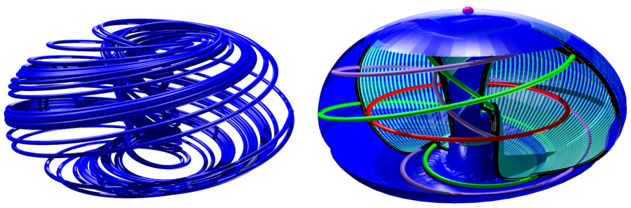
Figure 28: Visualization phase space structure: simulation versus invariant manifolds at $\alpha=0.9321$: Left: direct simulation of an initial condition for roughly one hundred time units. Right: the equilibrium solution $p_{0}$ (magenta dot), its unstable manifold (blue surface), the resonant torus comprised of a stable periodic orbit $\gamma_{1}$ (green curve), the saddle periodic orbit $\gamma_{2}$ (purple curve), and its unstable manifold (green torus). Also shown is the repelling periodic orbit $\gamma$ (red curve). Most of these objects have unstable directions and are impossible to locate by direct simulation. Even the attracting resonant torus is very difficult to “fill in” by just simulating the system.

6 Acknowledgments

The authors would like to thank Jordi-Lluís Figueras, Maciej Capiński, and Vincent Naudot for many helpful suggestions and invaluable insights. We owe also a special thanks to Takahito Mitsui for bringing the paper of Langford [20] to our attention after reading a much rougher early version of this manuscript. The published version of the manuscript benefitted greatly from the suggestions of two anonymous referees. The second author was partially supported by NSF grant DMS-1813501.

References

- [1] Ju. I. Neĭmark. Some cases of the dependence of periodic motions on parameters. Dokl. Akad. Nauk SSSR, 129:736–739, 1959.
- [2] Robert John Sacker. On invariant surfaces and bifurcation of periodic solutions of ordinary differential equations. ProQuest LLC, Ann Arbor, MI, 1964. Thesis (Ph.D.)–New York University.
- [3] Seung-hwan Kim, R. S. MacKay, and J. Guckenheimer. Resonance regions for families of torus maps. Nonlinearity, 2(3):391–404, 1989.
- [4] C. Baesens, J. Guckenheimer, S. Kim, and R. S. MacKay. Three coupled oscillators: mode-locking, global bifurcations and toroidal chaos. Phys. D, 49(3):387–475, 1991.
- [5] Kunihiko Kaneko. Transition from torus to chaos accompanied by frequency lockings with symmetry breaking. In connection with the coupled-logistic map. Progr. Theoret. Phys., 69(5):1427–1442, 1983.
- [6] V. S. Afraimovich and L. P. Shilńikov. Invariant two-dimensional tori, their breakdown and stochasticity. In Methods of the qualitative theory of differential equations, pages 3–26, 164. Gorḱov. Gos. Univ., Gorki, 1983.
- [7] D. V. Turaev and L. P. Shilńikov. Bifurcations of quasi-attractors of torus-chaos. In Mathematical mechanisms of turbulence (Russian), pages 113–121, iii. Akad. Nauk Ukrain. SSR, Inst. Mat., Kiev, 1986.
- [8] Renato C. Calleja, Alessandra Celletti, and Rafael de la Llave. Local behavior near quasi-periodic solutions of conformally symplectic systems. J. Dynam. Differential Equations, 25(3):821–841, 2013.
- [9] Renato C. Calleja, Alessandra Celletti, and Rafael de la Llave. A KAM theory for conformally symplectic systems: efficient algorithms and their validation. J. Differential Equations, 255(5):978–1049, 2013.
- [10] Marta Canadell and Àlex Haro. Computation of quasiperiodic normally hyperbolic invariant tori: rigorous results. J. Nonlinear Sci., 27(6):1869–1904, 2017.
- [11] Alain Chenciner. Bifurcations de points fixes elliptiques. I. Courbes invariantes. Inst. Hautes Etudes Sci. Publ. Math., (61):67–127, 1985.
- [12] A. Chenciner. Bifurcations de points fixes elliptiques. II. Orbites périodiques et ensembles de Cantor invariants. Invent. Math., 80(1):81–106, 1985.
- [13] Alain Chenciner. Bifurcations de points fixes elliptiques. III. Orbites périodiques de “petites” périodes et élimination résonnante des couples de courbes invariantes. Inst. Hautes Etudes Sci. Publ. Math., (66):5–91, 1988.
- [14] R. S. MacKay. Transport in D volume-preserving flows. J. Nonlinear Sci., 4(4):329–354, 1994.
- [15] Kunihiko Kaneko. Similarity structure and scaling property of the period-adding phenomena. Progr. Theoret. Phys., 69(2):403–414, 1983.
- [16] Kunihiko Kaneko. Collapse of tori and genesis of chaos in dissipative systems. World Scientific Publishing Co., Singapore, 1986.
- [17] Frank Schilder, Werner Vogt, Stephan Schreiber, and Hinke M. Osinga. Fourier methods for quasi-periodic oscillations. Internat. J. Numer. Methods Engrg., 67(5):629–671, 2006.
- [18] Marta Canadell and Àlex Haro. Parameterization method for computing quasi-periodic reducible normally hyperbolic invariant tori. In Advances in differential equations and applications, volume 4 of SEMA SIMAI Springer Ser., pages 85–94. Springer, Cham, 2014.
- [19] Marta Canadell and Àlex Haro. Computation of quasi-periodic normally hyperbolic invariant tori: algorithms, numerical explorations and mechanisms of breakdown. J. Nonlinear Sci., 27(6):1829–1868, 2017.
- [20] W. F. Langford. Numerical studies of torus bifurcations. In Numerical methods for bifurcation problems (Dortmund, 1983), volume 70 of Internat. Schriftenreihe Numer. Math., pages 285–295. Birkhäuser, Basel, 1984.
- [21] V. S. Afrauimovic, V. V. Bykov, and L. P. Silnikov. The origin and structure of the Lorenz attractor. Dokl. Akad. Nauk SSSR, 234(2):336–339, 1977.
- [22] V. I. Arnold, V. S. Afrajmovich, Yu. S. Ilyashenko, and L. P. Shilnikov. Bifurcation theory and catastrophe theory. Springer-Verlag, Berlin, 1999. Translated from the 1986 Russian original by N. D. Kazarinoff, Reprint of the 1994 English edition from the series Encyclopaedia of Mathematical Sciences [ıt Dynamical systems. V, Encyclopaedia Math. Sci., 5, Springer, Berlin, 1994; MR1287421 (95c:58058)].
- [23] Jacob Palis and Floris Takens. Hyperbolicity and sensitive chaotic dynamics at homoclinic bifurcations, volume 35 of Cambridge Studies in Advanced Mathematics. Cambridge University Press, Cambridge, 1993. Fractal dimensions and infinitely many attractors.
- [24] V. Araujo, M. J. Pacifico, E. R. Pujals, and M. Viana. Singular-hyperbolic attractors are chaotic. Trans. Amer. Math. Soc., 361(5):2431–2485, 2009.
- [25] X. Cabré, E. Fontich, and R. de la Llave. The parameterization method for invariant manifolds. I. Manifolds associated to non-resonant subspaces. Indiana Univ. Math. J., 52(2):283–328, 2003.
- [26] X. Cabré, E. Fontich, and R. de la Llave. The parameterization method for invariant manifolds. II. Regularity with respect to parameters. Indiana Univ. Math. J., 52(2):329–360, 2003.
- [27] X. Cabré, E. Fontich, and R. de la Llave. The parameterization method for invariant manifolds. III. Overview and applications. J. Differential Equations, 218(2):444–515, 2005.
- [28] Z.B. Stone and H.A. Stone. Imaging and quantifying mixing in a model droplet micromixer. Phys. Fluids, 17:063103, 2005. https://doi.org/10.1063/1.1929547.
- [29] K. E. Lenz, H. E. Lomelí, and J. D. Meiss. Quadratic volume preserving maps: an extension of a result of Moser. Regul. Chaotic Dyn., 3(3):122–131, 1998. J. Moser at 70 (Russian).
- [30] H. R. Dullin and J. D. Meiss. Quadratic volume-preserving maps: invariant circles and bifurcations. SIAM J. Appl. Dyn. Syst., 8(1):76–128, 2009.
- [31] Shawn C. Shadden, John O. Dabiri, and Jerrold E. Marsden. Lagrangian analysis of fluid transport in empirical vortex ring flows. Phys. Fluids, 18(4):047105, 11, 2006.
- [32] Takashi Matsumoto, Leon O. Chua, and Ryuji Tokunaga. Chaos via torus breakdown. IEEE Trans. Circuits and Systems, 34(3):240–253, 1987.
- [33] O. Sosnovtseva and E. Mosekilde. Torus destruction and chaos-chaos intermittency in a commodity distribution chain. Internat. J. Bifur. Chaos Appl. Sci. Engrg., 7(6):1225–1242, 1997.
- [34] Taoufik Bakri, Yuri A. Kuznetsov, and Ferdinand Verhulst. Torus bifurcations in a mechanical system. J. Dynam. Differential Equations, 27(3-4):371–403, 2015.
- [35] Taoufik Bakri and Ferdinand Verhulst. Bifurcations of quasi-periodic dynamics: torus breakdown. Z. Angew. Math. Phys., 65(6):1053–1076, 2014.
- [36] Vadim S. Anishchenko, Vladimir Astakhov, Alexander Neiman, Tatjana Vadivasova, and Lutz Schimansky-Geier. Nonlinear dynamics of chaotic and stochastic systems. Springer Series in Synergetics. Springer, Berlin, second edition, 2007. Tutorial and modern developments.
- [37] Arash Mohammadi. The Aizawa Attractor. https://www.youtube.com/watch?v=RBqbQUu-p00, November 2017.
- [38] Michael Gagliardo. 3d printing chaos. In Carlo Séquin Eve Torrence, Bruce Torrence and Kristóf Fenyvesi, editors, Proceedings of Bridges 2018: Mathematics, Art, Music, Architecture, Education, Culture, pages 491–494, Phoenix, Arizona, 2018. Tessellations Publishing. Available online at http://archive.bridgesmathart.org/2018/bridges2018-491.pdf.
- [39] http://chaoticatmospheres.com/mathrules-strange-attractors. “Strange Attractors.” Chaotic Atmospheres.
- [40] A. Haro and R. de la Llave. A parameterization method for the computation of invariant tori and their whiskers in quasi-periodic maps: rigorous results. J. Differential Equations, 228(2):530–579, 2006.
- [41] À. Haro and R. de la Llave. A parameterization method for the computation of invariant tori and their whiskers in quasi-periodic maps: numerical algorithms. Discrete Contin. Dyn. Syst. Ser. B, 6(6):1261–1300 (electronic), 2006.
- [42] A. Haro and R. de la Llave. A parameterization method for the computation of invariant tori and their whiskers in quasi-periodic maps: explorations and mechanisms for the breakdown of hyperbolicity. SIAM J. Appl. Dyn. Syst., 6(1):142–207 (electronic), 2007.
- [43] Gemma Huguet and Rafael de la Llave. Computation of limit cycles and their isochrons: fast algorithms and their convergence. SIAM J. Appl. Dyn. Syst., 12(4):1763–1802, 2013.
- [44] Antoni Guillamon and Gemma Huguet. A computational and geometric approach to phase resetting curves and surfaces. SIAM J. Appl. Dyn. Syst., 8(3):1005–1042, 2009.
- [45] J. D. Mireles James and Maxime Murray. Chebyshev-Taylor parameterization of stable/unstable manifolds for periodic orbits: implementation and applications. Internat. J. Bifur. Chaos Appl. Sci. Engrg., 27(14):1730050, 32, 2017.
- [46] Maxime Breden, Jean-Philippe Lessard, and Jason D. Mireles James. Computation of maximal local (un)stable manifold patches by the parameterization method. Indag. Math. (N.S.), 27(1):340–367, 2016.
- [47] Jan Bouwe van den Berg, Jason D. Mireles James, and Christian Reinhardt. Computing (un)stable manifolds with validated error bounds: non-resonant and resonant spectra. J. Nonlinear Sci., 26(4):1055–1095, 2016.
- [48] J. B. van den Berg and J. D. Mireles James. Parameterization of slow-stable manifolds and their invariant vector bundles: theory and numerical implementation. Discrete Contin. Dyn. Syst., 36(9):4637–4664, 2016.
- [49] William D. Kalies, Shane Kepley, and J. D. Mireles James. Analytic continuation of local (un)stable manifolds with rigorous computer assisted error bounds. SIAM J. Appl. Dyn. Syst., 17(1):157–202, 2018.
- [50] Jorge Gonzalez and J. D. Mireles James. High-order parameterization of stable/unstable manifolds for long periodic orbits of maps. SIAM Journal on Applied Dynamical Systems, 16(3):1748–1795, 2017. https://doi.org/10.1137/16M1090041.
- [51] Chris M. Groothedde and J. D. Mireles James. Parameterization method for unstable manifolds of delay differential equations. Journal of Computational Dynamics, pages 1–52, (First online September 2017). doi:10.3934/jcd.2017002.
- [52] Lei Zhang and Rafael de la Llave. Transition state theory with quasi-periodic forcing. Commun. Nonlinear Sci. Numer. Simul., 62:229–243, 2018.
- [53] Stavros Anastassiou, Anastasios Bountis, and Arnd Bäcker. Recent results on the dynamics of higher-dimensional Hénon maps. Regul. Chaotic Dyn., 23(2):161–177, 2018.
- [54] Stavros Anastassiou, Tassos Bountis, and Arnd Bäcker. Homoclinic points of 2D and 4D maps via the parametrization method. Nonlinearity, 30(10):3799–3820, 2017.
- [55] Àlex Haro, Marta Canadell, Jordi-Lluí s Figueras, Alejandro Luque, and Josep-Maria Mondelo. The parameterization method for invariant manifolds, volume 195 of Applied Mathematical Sciences. Springer, [Cham], 2016. From rigorous results to effective computations.
- [56] J. D. Mireles James. Validated numerics for equilibria of analytic vector fields: invariant manifolds and connecting orbits. Proceedings of Symposia in Applied Mathematics, 74:1–55, 2018.
- [57] Jan Bouwe van den Berg, J. D. Mireles James, Jean-Philippe Lessard, and Konstantin Mischaikow. Rigorous numerics for symmetric connecting orbits: even homoclinics of the Gray-Scott equation. SIAM J. Math. Anal., 43(4):1557–1594, 2011.
- [58] D. Ambrosi, G. Arioli, and H. Koch. A homoclinic solution for excitation waves on a contractile substratum. SIAM J. Appl. Dyn. Syst., 11(4):1533–1542, 2012.
- [59] Gianni Arioli and Hans Koch. Existence and stability of traveling pulse solutions of the FitzHugh-Nagumo equation. Nonlinear Anal., 113:51–70, 2015.
- [60] A. Wittig, M. Berz, J. Grote, K. Makino, and S. Newhouse. Rigorous and accurate enclosure of invariant manifolds on surfaces. Regul. Chaotic Dyn., 15(2-3):107–126, 2010.
- [61] C. Simo. On the Analytical and Numerical Approximation of Invariant Manifolds. In D. Benest and C. Froeschle, editors, Modern Methods in Celestial Mechanics, Comptes Rendus de la 13ieme Ecole Printemps d’Astrophysique de Goutelas (France), 24-29 Avril, 1989. Edited by Daniel Benest and Claude Froeschle. Gif-sur-Yvette: Editions Frontieres, 1990., p.285, page 285, 1990.
- [62] Bernd Krauskopf and Hinke Osinga. Two-dimensional global manifolds of vector fields. Chaos, 9(3):768–774, 1999.
- [63] Hinke Osinga. Non-orientable manifolds of periodic orbits. In International Conference on Differential Equations, Vol. 1, 2 (Berlin, 1999), pages 922–924. World Sci. Publ., River Edge, NJ, 2000.
- [64] John Guckenheimer and Alexander Vladimirsky. A fast method for approximating invariant manifolds. SIAM J. Appl. Dyn. Syst., 3(3):232–260, 2004.
- [65] A. Zanzottera, G. Mingotti, R. Castelli, and M. Dellnitz. Intersecting invariant manifolds in spatial restricted three-body problems: design and optimization of Earth-to-halo transfers in the Sun-Earth-Moon scenario. Commun. Nonlinear Sci. Numer. Simul., 17(2):832–843, 2012.
- [66] Michael Dellnitz and Andreas Hohmann. The computation of unstable manifolds using subdivision and continuation. In Nonlinear dynamical systems and chaos (Groningen, 1995), volume 19 of Progr. Nonlinear Differential Equations Appl., pages 449–459. Birkhäuser, Basel, 1996.
- [67] M. E. Henderson. Covering an invariant manifold with fat trajectories. In Model reduction and coarse-graining approaches for multiscale phenomena, pages 39–54. Springer, Berlin, 2006.
- [68] Michael E. Henderson. Computing invariant manifolds by integrating fat trajectories. SIAM J. Appl. Dyn. Syst., 4(4):832–882, 2005.
- [69] R. C. Calleja, E. J. Doedel, A. R. Humphries, A. Lemus-Rodríguez, and E. B. Oldeman. Boundary-value problem formulations for computing invariant manifolds and connecting orbits in the circular restricted three body problem. Celestial Mech. Dynam. Astronom., 114(1-2):77–106, 2012.
- [70] B. Krauskopf, H. M. Osinga, E. J. Doedel, M. E. Henderson, J. Guckenheimer, A. Vladimirsky, M. Dellnitz, and O. Junge. A survey of methods for computing (un)stable manifolds of vector fields. Internat. J. Bifur. Chaos Appl. Sci. Engrg., 15(3):763–791, 2005.
- [71] Roy H. Goodman and Jacek K. Wróbel. High-order bisection method for computing invariant manifolds of two-dimensional maps. Internat. J. Bifur. Chaos Appl. Sci. Engrg., 21(7):2017–2042, 2011.
- [72] Jacek K. Wróbel and Roy H. Goodman. High-order adaptive method for computing two-dimensional invariant manifolds of three-dimensional maps. Commun. Nonlinear Sci. Numer. Simul., 18(7):1734–1745, 2013.
- [73] Shane Kepley and J. D. Mireles James. Homoclinic dynamics in a restricted four body problem: a multi-parameter study of transverse connections for the saddle-focus equilibrium solutions. (submitted to Celestial Mechanics and Dynamical Astronomy), 2018.
- [74] S. Newhouse, J. Palis, and F. Takens. Bifurcations and stability of families of diffeomorphisms. Inst. Hautes Études Sci. Publ. Math., (57):5–71, 1983.
- [75] E. J. Doedel. Lecture notes on numerical analysis of bifurcation problems. In International Course on Bifurcations and Stability in Structural Engineering. Université Pierre et Marie Curie (Paris VI), November 2000.
- [76] H. B. Keller. Lectures on numerical methods in bifurcation problems, volume 79 of Tata Institute of Fundamental Research Lectures on Mathematics and Physics. Published for the Tata Institute of Fundamental Research, Bombay, 1987. With notes by A. K. Nandakumaran and Mythily Ramaswamy.
- [77] A. R. Champneys and Yu. A. Kuznetsov. Numerical detection and continuation of codimension-two homoclinic bifurcations. Internat. J. Bifur. Chaos Appl. Sci. Engrg., 4(4):785–822, 1994.
- [78] S. Smale. Differentiable dynamical systems. Bull. Amer. Math. Soc., 73:747–817, 1967.
- [79] S. Newhouse, D. Ruelle, and F. Takens. Occurrence of strange Axiom A attractors near quasiperiodic flows on ,. Comm. Math. Phys., 64(1):35–40, 1978/79.
- [80] Marcy Barge. Homoclinic intersections and indecomposability. Proc. Amer. Math. Soc., 101(3):541–544, 1987.
- [81] Judy Kennedy. How indecomposable continua arise in dynamical systems. In Papers on general topology and applications (Madison, WI, 1991), volume 704 of Ann. New York Acad. Sci., pages 180–201. New York Acad. Sci., New York, 1993.
- [82] Andreas Floer. A topological persistence theorem for normally hyperbolic manifolds via the Conley index. Trans. Amer. Math. Soc., 321(2):647–657, 1990.
- [83] Maciej J. Capiński and Hieronim Kubica. Persistence of normally hyperbolic invariant manifolds in the absence of rate conditions. (submitted), 2019.
- [84] W. F. Langford and G. Iooss. Interactions of Hopf and pitchfork bifurcations. In Bifurcation problems and their numerical solution (Proc. Workshop, Univ. Dortmund, Dortmund, 1980), volume 54 of Internat. Ser. Numer. Math., pages 103–134. Birkhäuser, Basel-Boston, Mass., 1980.
- [85] M. Golubitsky and D. Schaeffer. A theory for imperfect bifurcation via singularity theory. Comm. Pure Appl. Math., 32(1):21–98, 1979.
- [86] Martin Golubitsky, Ian Stewart, and David G. Schaeffer. Singularities and groups in bifurcation theory. Vol. II, volume 69 of Applied Mathematical Sciences. Springer-Verlag, New York, 1988.
- [87] Martin Golubitsky and William F. Langford. Classification and unfoldings of degenerate Hopf bifurcations. J. Differential Equations, 41(3):375–415, 1981.
- [88] Maciej J Capinski, Emmanuel Fleurantin, and J. D. Mireles James. Computer assisted proofs of two-dimensional attracting invariant tori for ODEs. arXiv:1905.08116.
- [89] Jan Bouwe van den Berg, Andréa Deschênes, Jean-Philippe Lessard, and Jason D. Mireles James. Stationary coexistence of hexagons and rolls via rigorous computations. SIAM J. Appl. Dyn. Syst., 14(2):942–979, 2015.
- [90] Daniel Wilczak and Piotr Zgliczynski. -lohner algorithm. Scheade Informaticae, 20:9–46, 2011.
- [91] Daniel Wilczak and Piotr Zgliczynski. Heteroclinic connections between periodic orbits in planar restricted circular three-body problem—a computer assisted proof. Comm. Math. Phys., 234(1):37–75, 2003.
- [92] Daniel Wilczak. Symmetric homoclinic solutions to the periodic orbits in the Michelson system. Topol. Methods Nonlinear Anal., 28(1):155–170, 2006.
- [93] Gianni Arioli and Piotr Zgliczyński. Symbolic dynamics for the Hénon-Heiles Hamiltonian on the critical level. J. Differential Equations, 171(1):173–202, 2001.
- [94] Maciej J. Capiński and Anna Wasieczko-Zajac. Geometric proof of strong stable/unstable manifolds with application to the restricted three body problem. Topol. Methods Nonlinear Anal., 46(1):363–399, 2015.
- [95] Maciej J. Capiński. Computer assisted existence proofs of Lyapunov orbits at and transversal intersections of invariant manifolds in the Jupiter-Sun PCR3BP. SIAM J. Appl. Dyn. Syst., 11(4):1723–1753, 2012.
- [96] Daniel Wilczak. The existence of Shilnikov homoclinic orbits in the Michelson system: a computer assisted proof. Found. Comput. Math., 6(4):495–535, 2006.
- [97] Daniel Wilczak. Symmetric heteroclinic connections in the Michelson system: a computer assisted proof. SIAM J. Appl. Dyn. Syst., 4(3):489–514 (electronic), 2005.
- [98] Zin Arai, William Kalies, Hiroshi Kokubu, Konstantin Mischaikow, Hiroe Oka, and Paweł Pilarczyk. A database schema for the analysis of global dynamics of multiparameter systems. SIAM J. Appl. Dyn. Syst., 8(3):757–789, 2009.
- [99] Tomoyuki Miyaji, PawełPilarczyk, Marcio Gameiro, Hiroshi Kokubu, and Konstantin Mischaikow. A study of rigorous ODE integrators for multi-scale set-oriented computations. Appl. Numer. Math., 107:34–47, 2016.
- [100] Jordi-Lluís Figueras, Alex Haro, and Alejandro Luque. Rigorous computer assisted application of kam theory: a modern approach. (Submitted) arXiv:1601.00084 [math.DS], 2016.