Abstract

We consider flux vacua for type IIB orientifold compactifications and study their interplay with the tadpole-cancellation condition. As a concrete example we focus on $\mathbb{T}^{6}/\mathbb{Z}_{2}\times\mathbb{Z}_{2}$, for which we find that solutions to the F-term equations at weak coupling, large complex structure and large volume require large flux contributions. Such contributions are however strongly disfavored by the tadpole-cancellation condition. We furthermore find that solutions which stabilize moduli in this perturbatively-controlled regime are only a very small fraction of all solutions, and that the space of solutions is not homogenous but shows characteristic void structures and vacua concentrated on submanifolds.

1 Introduction

String theory is argued to be a consistent theory of quantum gravity including gauge interactions. It is defined in ten space-time dimensions, and in order to make a connection to four-dimensional physics six spatial dimensions have to be compactified. Such compactifications have to satisfy a number of consistency conditions, for instance, in the presence of D-branes and closed-string fluxes the tadpole-cancellation condition and the Freed-Witten anomaly-cancellation condition have to be satisfied. (For a review of the former see [1] and for the latter see [2].) These conditions relate the closed- and open-string sectors to each other and put strong restrictions on the allowed background configurations. More concretely,

1. compactifications of string theory to four dimensions are typically performed on Calabi-Yau three-folds. The resulting effective theory contains a number of massless scalar fields corresponding to deformations of the background, which should be absent due to experimental constraints. A way to achieve this for type II theories is to deform the background geometry by Neveu-Schwarz–Neveu-Schwarz (NS-NS) and Ramond-Ramond (R-R) fluxes, which generate a potential in the four-dimensional theory and provide mass-terms for the moduli fields. This procedure is called moduli stabilization, and for early work in the type IIB context see for instance [3, 4, 5] and for work in the type IIA context see [6, 7, 8]. However, especially in the type IIB setting some of the moduli cannot be stabilized by (geometric) fluxes. One therefore includes non-perturbative effects which lead to the KKLT [9] and large-volume [10] scenarios. Moduli stabilization often results in anti-de-Sitter or Minkowski vacua, while it is difficult to obtain de-Sitter solutions [11].

2. A gauge-theory sector for type II theories can be engineered using D-branes. D-branes filling four-dimensional space-time and wrapping submanifolds in the compact space have a gauge theory localized on their world-volume. Chiral matter can be localized at the intersection loci of different D-branes in the compact space, and in this way four-dimensional gauge theories can be constructed in a geometric way (for a review see for instance [1]). However, when introducing D-branes one typically has to perform an orientifold projection of the theory. The fixed-loci of this projection correspond to orientifold planes which generically have negative mass and negative charge.

Moduli stabilization and the construction of a gauge-theory sector are two important aspects of connecting string theory to realistic four-dimensional physics. These tasks are often approached independently, however, as emphasized for instance in [12], there is a complicated interplay between them. This interplay can prevent moduli from being stabilized or can modify the stabilization procedure. Following this line of thought, the purpose of this paper is to study how parts 1) and 2) are connected via the tadpole-cancellation condition (schematically)

$$\begin{split}\mbox{fluxes}=\mbox{D-branes}+\mbox{O-planes}\,.\end{split}$$ (1.1)

We approach this question by analyzing how properties of the space of flux vacua depends on the contribution of fluxes to the left-hand side of (1.1). We perform our analysis for the type IIB orientifold of $\mathbb{T}^{6}/\mathbb{Z}_{2}\times\mathbb{Z}_{2}$, and consider R-R three-form flux, geometric NS-NS $H$-flux as well as non-geometric NS-NS $Q$-flux. The geometric fluxes generically stabilize the complex-structure moduli and the axio-dilaton, while the non-geometric fluxes allow for stabilization of the Kähler moduli. We then determine distributions for how the values of the stabilized moduli depend on the tadpole contribution of the fluxes. Note that distributions of flux vacua have been discussed extensively in the literature before. For instance, for type IIB compactifications various aspects have been studied in [13, 14, 15, 16, 17, 18, 19, 20, 21, 22, 23, 24] and for type IIA related work can be found in [8, 25]. In the context of M-theory similar questions have been discussed in [26], and for F-theory see [27]. Recently also topological data analysis has been used to investigate properties of flux vacua in [28, 29]. The main results of our analysis can be summarized as follows:

• We observe that the space of flux vacua is not homogenous but shows characteristic structures such as circular voids [16]. We show furthermore that solutions can be accumulated on submanifolds in the space of solutions.

• We find that flux configurations which stabilize moduli in a weak-coupling, large complex-structure and/or large-volume regime are only a very small fraction of all possible configurations. The number of reliable flux vacua is therefore much smaller than naively expected.

• In order to stabilize moduli in a weak-coupling, large complex-structure and large-volume regime, the flux contribution to the left-hand side of tadpole-cancellation condition (1.1) has to be larger than a certain threshold. The more reliable these vacua are required to be, the larger this threshold has to be. However, the contribution of D-branes and orientifold planes to the right-hand side of (1.1) is typically small. It is therefore difficult to perform moduli stabilization in a perturbatively-controlled regime and to satisfy the tadpole-cancellation condition.

Our findings for the structure of the space of flux vacua agree with for instance [16, 29] for the axio-dilaton, but we extend their analysis by including the complex-structure moduli. Our observation concerning the difficulty of obtaining reliable flux vacua is consistent with for instance [30], who find that type IIB solutions at weak string-coupling are rare. Similarly, in [31] the authors argue that in order to avoid a certain runaway behaviour large fluxes have to be considered, also in [32] large fluxes are needed to obtain reliable solutions, and related difficulties are encountered in [33].

This work is organized as follows: in section 2 we review type IIB orientifold compactifications with geometric and non-geometric fluxes, we discuss the corresponding tadpole-cancellation conditions, we specialize to the example of the $\mathbb{T}^{6}/\mathbb{Z}_{2}\times\mathbb{Z}_{2}$ orientifold and determine the relevant dualities. In section 3 we study moduli stabilization for the axio-dilaton, in section 4 we discuss the combined moduli stabilization of the axio-dilaton and the complex-structure moduli, and in section 5 we stabilize all of the closed-string moduli at tree-level. At the end of sections 3, 4 and 5 we have included brief summaries for each section, which may help the reader to get an overview of the main results. Our conclusions can be found in section 6.

2 Flux compactifications

In this paper we are interested in compactifications of type IIB string theory on Calabi-Yau orientifolds with geometric and non-geometric fluxes. In order to fix our notation, we start in sections 2.1 and 2.2 by briefly reviewing orientifold compactifications and tadpole-cancellation conditions for general Calabi-Yau three-folds. In section 2.3 we specialize to the example of $\mathbb{T}^{6}/\mathbb{Z}_{2}\times\mathbb{Z}_{2}$, and in section 2.4 we discuss duality transformations for this background.

2.1 Orientifold compactifications

Type IIB orientifold compactifications on Calabi-Yau three-folds give rise to a $\mathcal{N}=1$ supergravity theory in four dimensions. This theory can be characterized in terms of a superpotential, Kähler potential and D-term potential, which we determine in the following.

Calabi-Yau orientifolds

We begin with type IIB string theory on $\mathbb{R}^{3,1}\times\mathcal{X}$, where $\mathcal{X}$ denotes a Calabi-Yau three-fold. The latter comes with a holomorphic three-form $\Omega\in H^{3,0}(\mathcal{X})$ and a real Kähler form $J\in H^{1,1}(\mathcal{X})$, and to perform an orientifold projection we impose a holomorphic involution $\sigma$ on $\mathcal{X}$ which acts on $\Omega$ and $J$ as

$$\begin{split}\sigma^{*}J=+J\,,\hskip 60.0pt\sigma^{*}\hskip 1.0pt\Omega=-\Omega\,.\end{split}$$ (2.1)

The involution leaves the non-compact four-dimensional part invariant, and hence the fixed loci of $\sigma$ correspond to orientifold three- and seven planes. For the full orientifold projection $\sigma$ is combined with $\Omega_{\rm P}(-1)^{F_{\rm L}}$, where $\Omega_{\rm P}$ denotes the world-sheet parity operator and $F_{\rm L}$ is the left-moving fermion number. The latter two act on the bosonic fields in the following way

$$\begin{split}\begin{array}[]{lclclcl}\displaystyle\Omega_{\rm P}\,(-1)^{F_{\rm L}}\>g&=&+\>g\,,&&\displaystyle\Omega_{\rm P}\,(-1)^{F_{\rm L}}\>B&=&-B\,,\\[6.0pt] \displaystyle\Omega_{\rm P}\,(-1)^{F_{\rm L}}\>\phi&=&+\>\phi\,,&&\displaystyle\Omega_{\rm P}\,(-1)^{F_{\rm L}}\>C_{2p}&=&(-1)^{p}\,C_{2p}\,,\end{array}\end{split}$$ (2.2)

with $g$ the metric, $B$ the Kalb-Ramond field, $\phi$ the dilaton and $C_{2p}$ the Ramond-Ramond potentials in type IIB. Since $\sigma$ is an involution, the cohomology groups of the Calabi-Yau three-fold $\mathcal{X}$ split into even and odd eigenspaces as $H^{p,q}(\mathcal{X})=H^{p,q}_{+}(\mathcal{X})\oplus H^{p,q}_{-}(\mathcal{X})$ [34], and for the discussion in this paper we assume that the corresponding Hodge numbers satisfy

$$\begin{split}h^{2,1}_{+}=0\,,\hskip 50.0pth^{1,1}_{-}=0\,.\end{split}$$ (2.3)

However, more general cases can be considered as well. For the third de-Rham cohomology group $H^{3}_{-}(\mathcal{X})$ we choose a symplectic basis as follows

$$\begin{split}\{\alpha_{I},\beta^{I}\}\,,\hskip 50.0pt\int_{\mathcal{X}}\alpha_{I}\wedge\beta^{J}=\delta_{I}{}^{J}\,,\hskip 50.0ptI,J=0,\ldots,h^{2,1}_{-}\,,\end{split}$$ (2.4)

with all other pairings vanishing. For the even Dolbeault cohomology groups we introduce bases

$$\begin{split}\begin{array}[]{rclcl}|g_{\mathcal{X}}|^{-1/2}d\mbox{vol}_{\mathcal{X}}&=&\omega_{0}&\in&H^{3,3}_{+}(\mathcal{X})\,,\\ &&\omega_{\mathsf{A}}&\in&H^{1,1}_{+}(\mathcal{X})\,,\\ &&\sigma^{\mathsf{A}}&\in&H^{2,2}_{+}(\mathcal{X})\,,\\ 1&=&\sigma^{0}&\in&H^{0,0}_{+}(\mathcal{X})\,,\end{array}\hskip 50.0pt\mathsf{A}=1,\ldots,h^{1,1}_{+}\,,\end{split}$$ (2.5)

where $|g_{\mathcal{X}}|$ denotes the determinant of the metric for $\mathcal{X}$. These bases can be chosen such that they satisfy a condition analogous to (2.4), in particular, we can require

$$\begin{split}\{\omega_{A},\sigma^{A}\}\,,\hskip 50.0pt\int_{\mathcal{X}}\omega_{A}\wedge\sigma^{B}=\delta_{A}{}^{B}\,,\hskip 50.0ptA,B=0,\ldots,h^{1,1}_{+}\,.\end{split}$$ (2.6)

Moduli

When compactifying string theory from ten to four dimensions, the deformations of the six-dimensional background become dynamical fields in the four-dimensional theory. These moduli fields are contained in the multiforms [35]

$$\begin{split}\begin{array}[]{lcl}\Phi^{+}&=&\displaystyle e^{-\phi}\,e^{B-i\hskip 1.0ptJ}\,,\\[4.0pt] \Phi^{-}&=&\Omega\,,\end{array}\hskip 60.0pt\Phi^{+}_{\rm c}=e^{B}\hskip 1.0pt\mathcal{C}_{\rm mod}+i\,\mbox{Re}\hskip 1.0pt\Phi^{+}\,,\end{split}$$ (2.7)

where the sum over all R-R potentials $\mathcal{C}=\sum_{p}C_{p}$ has been separated into a flux contribution and a moduli contribution as $\mathcal{C}=\mathcal{C}_{\rm flux}+\mathcal{C}_{\rm mod}$. Complex scalar fields $\tau$ and $T_{\mathsf{A}}$ can be determined by expanding $\Phi^{+}_{\rm c}$ into its zero- and four-form components as follows

$$\begin{split}\Phi^{+}_{\rm c}=\tau+T_{\mathsf{A}}\hskip 1.0pt\sigma^{\mathsf{A}}\equiv T_{A}\hskip 1.0pt\sigma^{A}\,,\end{split}$$ (2.8)

where $T_{0}\equiv\tau$ is called the axio-dilaton and $T_{\mathsf{A}}$ contain the Kähler moduli of $\mathcal{X}$. In general this expression also contains two-forms anti-invariant under $\sigma$, which are however vanishing due to our choice (2.3). The complex-structure moduli $U^{i}$ with $i=1,\ldots,h^{2,1}_{-}$ are contained in the holomorphic three-form $\Omega$.

Fluxes

We furthermore consider non-vanishing fluxes for the internal space. These are the R-R three-form flux $F=d\hskip 1.0pt\mathcal{C}_{\rm flux}\bigr{\rvert}_{3}$ as well as geometric and non-geometric fluxes in the NS-NS sector. The latter are the three-form flux $H$, the geometric flux $f$, and the non-geometric $Q$- and $R$-fluxes. These fluxes can be interpreted as operators acting on the differential forms as

$$\begin{split}\begin{array}[]{l@{\hspace{7pt}}c@{\hspace{12pt}}lcl}H\,\wedge\hfil\hskip 7.0&:\hfil\hskip 12.0&\mbox{$p$-form}&\to&\mbox{$(p+3)$-form}\,,\\ f\hskip 4.5pt\circ\hfil\hskip 7.0&:\hfil\hskip 12.0&\mbox{$p$-form}&\to&\mbox{$(p+1)$-form}\,,\\ Q\,\bullet\hfil\hskip 7.0&:\hfil\hskip 12.0&\mbox{$p$-form}&\to&\mbox{$(p-1)$-form}\,,\\ R\,\llcorner\hfil\hskip 7.0&:\hfil\hskip 12.0&\mbox{$p$-form}&\to&\mbox{$(p-3)$-form}\,,\end{array}\end{split}$$ (2.9)

and can be conveniently summarized using a generalized derivative operator [36]

$$\begin{split}\mathcal{D}=d+H\wedge-f\circ+Q\bullet-R\hskip 1.0pt\llcorner\,.\end{split}$$ (2.10)

The precise action of the fluxes on the cohomology will be specified below. We furthermore summarize the action of the combined world-sheet parity and left-moving fermion number on the fluxes as follows [36, 37]

$$\begin{split}\begin{array}[]{lccl}\Omega_{\rm P}(-1)^{F_{\rm L}}\,H&=&-&H\,,\\[4.0pt] \Omega_{\rm P}(-1)^{F_{\rm L}}\,f&=&+&f\,,\\[4.0pt] \Omega_{\rm P}(-1)^{F_{\rm L}}\,Q&=&-&Q\,,\\[4.0pt] \Omega_{\rm P}(-1)^{F_{\rm L}}\,R&=&+&R\,.\end{array}\hskip 50.0pt\Omega_{\rm P}(-1)^{F_{\rm L}}\,F=-F\,,\end{split}$$ (2.11)

For our assumption (2.3) this implies that $f$ and $R$ are vanishing. We also note that the R-R and NS-NS three-form fluxes have to satisfy quantization conditions of the form (see e.g. [38])

$$\begin{split}\int_{\Gamma}F\in\mathbb{Z}\,,\hskip 60.0pt\int_{\Gamma}H\in\mathbb{Z}\,,\end{split}$$ (2.12)

where $\Gamma\in H_{3}(\mathcal{X},\mathbb{Z})$ is an arbitrary three-cycle on the Calabi-Yau three-fold $\mathcal{X}$. For orbifolds and orientifolds this condition can be modified, and we come back to this point on page 2.3 below. Furthermore, as will be explained in section 2.4, the NS-NS fluxes are related among each other through T-duality transformations, and hence also the geometric $f$- and the non-geometric $Q$- and $R$-fluxes should be appropriately quantized.

Supergravity data

When compactifying type IIB string theory on orientifolds of Calabi-Yau three-folds, the resulting four-dimensional effective theory can be described in terms of $\mathcal{N}=1$ supergravity [34]. In particular, the Kähler potential takes the following form

$$\begin{split}&\mathcal{K}=-\log\bigl{[}-i\hskip 1.0pt(\tau-\overline{\tau})\bigr{]}-2\log\hat{\mathcal{V}}-\log\biggl{[}-i\int_{\mathcal{X}}\Omega\wedge\overline{\Omega}\,\biggr{]}\,,\end{split}$$ (2.13)

where $\hat{\mathcal{V}}$ denotes the volume of the Calabi-Yau manifold in Einstein frame. The superpotential is generated by the fluxes and can be expressed using the Mukai pairing $\langle\cdot,\cdot\rangle$ of the multiforms (2.7) and the generalized derivative (2.10) in the following way [36, 39, 23]

$$\begin{split}W=&\int_{\mathcal{X}}\bigl{\langle}\Phi^{-},F-\mathcal{D}\hskip 1.0pt\Phi^{+}_{\rm c}\bigr{\rangle}\\[4.0pt] =&\int_{\mathcal{X}}\Omega\wedge\Bigl{[}F-\tau\hskip 1.0ptH-\bigl{(}Q\bullet\sigma^{\mathsf{A}}\bigr{)}\hskip 1.0ptT_{\mathsf{A}}\Bigr{]}.\end{split}$$ (2.14)

In general, the fluxes (2.9) also generate a D-term potential which can be expressed using the three-form part of $\mathcal{D}(\mbox{Im}\hskip 1.0pt\Phi^{+})$ [37] (see also [40]). However, due to (2.11) the latter belongs to the $\sigma$-even third cohomology and vanishes when taking into account our requirements (2.3). In our setting therefore no D-term potential is generated.

Bianchi identities and tadpole-cancellation conditions

Finally, the R-R and NS-NS fluxes have to satisfy a number of Bianchi identities. These can be expressed using the generalized derivative $\mathcal{D}$ as follows

$$\begin{split}\mathcal{D}^{2}=\mbox{NS-NS sources}\,,\hskip 50.0pt\mathcal{D}F=\mbox{R-R sources}\,,\end{split}$$ (2.15)

where NS-NS sources stand for NS5-branes, Kaluza-Klein monopoles or non-geometric $5^{2}_{2}$-branes (see for instance [41] for a review and collection of references). However, in this work we assume these to be absent and therefore require $\mathcal{D}^{2}=0$. The R-R sources stand for orientifold planes and D-branes, and the second condition in (2.15) is also known as the tadpole cancellation condition. We discuss this condition in more detail in the following section.

2.2 Tadpole-cancellation condition

The tadpole-cancellation condition is an important consistency conditions for type I string theories. It links the closed-string to the open-string sector and puts strong constraints on the allowed D-brane configurations (for a review see for instance [1]). From a conformal-field-theory point of view the tadpole-cancellation condition ensures the absence of UV divergencies in one-loop amplitudes (see e.g. [42, 43] for textbook reviews) and therefore plays an important role for string theory being a consistent theory of gravity. From an effective-field-theory point of view, the tadpole-cancellation condition is the integrated version of the equation of motion for the R-R potentials and ensures the absence of certain anomalies in type II orientifold compactifications via the generalized Green-Schwarz mechanism [44]. The tadpole-cancellation condition is thus an important consistency condition for string compactifications.

Explicit expressions

We now formulate the tadpole-cancellation condition for the setting of the previous section. The contribution of the R-R-sources can be described using the charges [45, 46]

$$\begin{split}\mathcal{Q}_{{\rm D}p}=\mbox{ch}\left(\mathcal{F}\right)\wedge\sqrt{\frac{\hat{\mathcal{A}}(\mathcal{R}_{T})}{\hat{\mathcal{A}}(\mathcal{R}_{N})}}\wedge[\Gamma_{{\rm D}p}]\,,\hskip 30.0pt\mathcal{Q}_{{\rm O}p}=Q_{p}\sqrt{\frac{\mathcal{L}(\mathcal{R}_{T}/4)}{\mathcal{L}(\mathcal{R}_{N}/4)}}\wedge[\Gamma_{{\rm O}p}]\,,\end{split}$$ (2.16)

where $[\Gamma_{{\rm D}p}]$ and $[\Gamma_{{\rm O}p}]$ denote the Poincaré duals of the cycles wrapped by D-branes and O-planes in $\mathbb{R}^{1,3}\times\mathcal{X}$. The open-string gauge flux on the D-branes $\mathcal{F}$ appears in the Chern character, the tangential and normal part of the curvature two-form $\mathcal{R}$ appear in the $\hat{\mathcal{A}}$-genus and the Hirzebruch polynomial $\mathcal{L}$, and $Q_{p}=-2^{p-4}$ denotes the charge of an orientifold $p$-plane. For more details we refer for instance to section 8.6 in [41]. Denoting the orientifold image of a D$p$-brane with a prime, the Bianchi identity for the R-R fluxes then reads

$$\begin{split}\mathcal{D}F=\sum_{{\rm D}p+{\rm D}p^{\prime}}\mathcal{Q}_{{\rm D}p}+\sum_{{\rm O}p}\mathcal{Q}_{{\rm O}p}\,,\end{split}$$ (2.17)

where the sum is over all D-branes and orientifold planes present in the background. The Freed-Witten anomaly-cancellation condition [2] for D-branes takes the general form [47, 41]

$$\begin{split}\mathcal{D}\mathcal{Q}_{{\rm D}p}=0\,,\hskip 50.0pt\mathcal{D}\mathcal{Q}_{{\rm O}p}=0\,,\end{split}$$ (2.18)

where we included the corresponding expression for an orientifold $p$-plane. Equation (2.17) can therefore be interpreted as a relation in $\mathcal{D}$-cohomology.

For the setting discussed in this paper, the orientifold projection satisfies (2.1) and therefore leads to spacetime filling O3- and O7-planes. Taking into account (2.3) and that $F$ in (2.17) is a three-form flux, we find the following explicit expressions

$$\begin{split}Q\bullet F=&-2\hskip 1.0pt\sum_{{\rm D}7_{a}}N_{{\rm D}7_{a}}[\Gamma_{{\rm D}7_{a}}]+8\sum_{{\rm O}7_{b}}\,[\Gamma_{{\rm O}7_{b}}]\,,\\[6.0pt] H\wedge F=&-2\left(N_{{\rm D}3}-\frac{N_{{\rm O}3}}{4}\right)\omega_{0}\\ &-\sum_{{\rm D}7_{a}}\mbox{tr}\bigl{(}\mathcal{F}_{a}\bigr{)}^{2}\wedge[\Gamma_{{\rm D}7_{a}}]+2\left(\sum_{{\rm D}7_{a}}N_{{\rm D}7_{a}}\>\frac{\chi(\Gamma_{{\rm D}7_{a}}\bigr{)}}{24}+\sum_{{\rm O}7_{b}}\frac{\chi\bigl{(}\Gamma_{{\rm O}7_{b}}\bigr{)}}{12}\right)\omega_{0}\,.\end{split}$$ (2.19)

Here, $N_{{\rm D}3}$ and $N_{{\rm O}3}$ denote the number of D$3$-branes and O$3$-planes, $N_{{\rm D}7_{a}}$ denotes the number of coincident D$7$-branes in a stack $a$, $[\Gamma_{{\rm D}7_{a}}]=n_{a}^{\mathsf{A}}\omega_{\mathsf{A}}$ is the Poincaré dual of the cycle $\Gamma_{{\rm D}7_{a}}$ expanded in the basis (2.5), $\mathcal{F}_{a}$ is the (quantized) two-form gauge flux on the stack of D$7$-branes $a$ in the fundamental representation, and $\chi(\Gamma)$ denotes the Euler number of the cycle $\Gamma$. The D-brane sums are over all D7-branes, and due to $h^{1,1}_{-}=0$ the orientifold images give a factor of two. For details on the derivation of these expressions see for instance [48].

Orientifold contributions

Let us now discuss the contribution of orientifold planes to the right-hand sides in (2.19). Typically orientifold planes give a positive contribution while D-branes give a negative contribution. For some classes of models the orientifold-contributions can be estimated as follows:

• For orientifolds of $\mathbb{T}^{6}/\mathbb{Z}_{M}$ or $\mathbb{T}^{6}/\mathbb{Z}_{M}\times\mathbb{Z}_{N}$ the numbers of O$3$- and O$7$-planes have been computed for instance in [49] for some examples. Here, the authors find that $N_{{\rm O}3},N_{{\rm O}7}\lesssim 60$ and the contribution of the Euler numbers to (2.19) are vanishing. The contribution of orientifold planes to the right-hand sides of (2.19) is therefore typically positive and of order $\mathcal{O}(10)$.

• For del-Pezzo surfaces the possible orientifold projections have been classified in [50]. The number of orientifold three- and seven-planes are of order $\mathcal{O}(10)$, and in some examples the Euler numbers of the four-cycles are of order $\mathcal{O}(100)$. Also here, the contribution of orientifold planes to the right-hand side of (2.19) is positive and of order $\mathcal{O}(10)$.

• In F-theory the geometry of Calabi-Yau four-folds $\mathcal{Y}$ encodes the geometry of D$7$-branes and orientifold planes in Calabi-Yau three-folds $\mathcal{X}$. If a lift from type IIB orientifolds to F-theory is possible, one finds that

  $$\begin{split}\frac{\chi(\mathcal{Y})}{24}=\frac{N_{{\rm O}3}}{4}+\sum_{{\rm D}7_{a}}N_{{\rm D}7_{a}}\hskip 1.0pt\frac{\chi(\Gamma_{{\rm D}7_{a}}\bigr{)}}{24}+\sum_{{\rm O}7_{b}}\frac{\chi\bigl{(}\Gamma_{{\rm O}7_{b}}\bigr{)}}{12}\,,\end{split}$$ (2.20)

  where $\chi(\mathcal{Y})$ denotes the Euler number of the Calabi-Yau four-fold $\mathcal{Y}$. In [51, 52] a manifold $\mathcal{Y}_{\rm max}$ was identified with the largest known Euler number for a Calabi-Yau four-fold

  $$\begin{split}\chi(\mathcal{Y}_{\rm max})=1\,820\,448\,,\end{split}$$ (2.21)

  and more details for the present context can be found in [53]. Hence, for this example the contribution to the D$3$-tadpole in (2.19) is of order $\mathcal{O}(10^{5})$.

D-brane contributions

We furthermore note that the tadpole-cancellation conditions (2.19) are the integrated versions of the R-R Bianchi identities (2.15). The former are therefore less restrictive than the latter, but for a proper string-theory solution also the Bianchi identities with localized sources have to be solved. When placing D-branes directly on top of orientifold planes solutions may be constructed more easily, but in general this a difficult task (see for instance [54]).

However, we can make the following general argument: because D-branes have a non-vanishing mass, their probe approximation breaks down when too many D-branes are placed into a compact space (away from the orientifold planes). In this case the back-reaction of D-branes on the geometry has to be taken into account, and an extreme case for this mechanism is the formation of black holes. It would be desirable to make this more precise, but we can argue that for ignoring back-reaction effects the contribution of D-branes to the right-hand sides in (2.19) should not be arbitrarily large.

Flux contributions

Turning now to the flux contribution on the left-hand sides in (2.19), we note that for vanishing $Q$-flux the $H\wedge F$-term typically has to be positive in order to obtain physically-relevant solutions. Since the right-hand sides are bounded from above by the orientifold contributions, the flux contributions should not be larger than $\mathcal{O}(10)$ to $\mathcal{O}(10^{5})$. In the presence of non-geometric $Q$-flux the left-hand sides in (2.19) can be negative – but since also the D-brane contributions are bounded, again the flux contributions should not be too large. This is an important point for our approach in this paper, which we summarize as

In order to solve the tadpole-cancellation condition (2.19) and ignore the back-reaction of D-branes, the contribution of fluxes to the left-hand sides in (2.19) should not be too large. Depending on the setting, known bounds are of orders $\mathcal{O}(10)$ to $\mathcal{O}(10^{5})$.

2.3 $\mathbb{T}^{6}/\mathbb{Z}_{2}\times\mathbb{Z}_{2}$ orientifold

Let us now turn to a specific example for a compactification space. We consider the orbifold $\mathbb{T}^{6}/\mathbb{Z}_{2}\times\mathbb{Z}_{2}$ which provides a simple example of a Calabi-Yau three-fold with only few moduli. For our purposes it is sufficient to stay in the orbifold limit and not blow-up the fixed-point singularities, that is we ignore the twisted sectors. This model has been extensively studied in the literature, and we refer for instance to [55, 56, 57, 58] for more details in the present context.

For this model the contribution of orientifold planes to the tadpole-cancellation condition (2.19) only allows for a small number of different flux choices. In order to be able to study general properties of the space of solutions, in the following we therefore ignore the precise form of the tadpole cancellation condition and allow for arbitrarily-large values of $H\wedge F$ and $Q\bullet F$. We do however keep in mind that these tadpole contributions are bounded by the D-brane and orientifold contributions.

Compactification space

We start from the following six-dimensional orbifold construction which has the properties of a Calabi-Yau three-fold

$$\begin{split}\mathcal{X}=\frac{\mathbb{T}^{2}\times\mathbb{T}^{2}\times\mathbb{T}^{2}}{\mathbb{Z}_{2}\times\mathbb{Z}_{2}}\,.\end{split}$$ (2.22)

On each of the two-tori we introduce complex coordinates as

$$\begin{split}z^{i}=x^{i}+U^{i}\hskip 1.0pty^{i}\,,\hskip 50.0pti=1,2,3\,,\end{split}$$ (2.23)

where $x^{i}$ and $y^{i}$ denote real coordinates with identifications $x^{i}\sim x^{i}+1$ and $y^{i}\sim y^{i}+1$, $U^{i}$ denote the complex structures on each of the $\mathbb{T}^{2}$, and no summation is performed in (2.23). The orbifold action is given by

$$\begin{split}\Theta:\left(\begin{array}[]{c}z_{1}\\ z_{2}\\ z_{3}\end{array}\right)\rightarrow\left(\begin{array}[]{c}-z_{1}\\ -z_{2}\\ +z_{3}\end{array}\right),\hskip 50.0pt\Theta^{\prime}:\left(\begin{array}[]{c}z_{1}\\ z_{2}\\ z_{3}\end{array}\right)\rightarrow\left(\begin{array}[]{c}+z_{1}\\ -z_{2}\\ -z_{3}\end{array}\right),\end{split}$$ (2.24)

where $\Theta$ and $\Theta^{\prime}$ are the two generators of the orbifold group $\mathbb{Z}_{2}\times\mathbb{Z}_{2}$. In addition, we perform the following orientifold projection

$$\begin{split}\sigma:\left(\begin{array}[]{c}z_{1}\\ z_{2}\\ z_{3}\end{array}\right)\rightarrow\left(\begin{array}[]{c}-z_{1}\\ -z_{2}\\ -z_{3}\end{array}\right).\end{split}$$ (2.25)

Cohomology

Next, we turn to the cohomology of (2.22). We note that there are no one- or five-forms invariant under the orbifold action (2.24), and that the invariant three-forms are given by the following combinations

$$\begin{split}\begin{array}[]{lcl@{\hspace{50pt}}lcl}\alpha_{0}&=&dx^{1}\wedge dx^{2}\wedge dx^{3}\,,\hfil\hskip 50.&\beta^{0}&=&+dy^{1}\wedge dy^{2}\wedge dy^{3}\,,\\[4.0pt] \alpha_{1}&=&dy^{1}\wedge dx^{2}\wedge dx^{3}\,,\hfil\hskip 50.&\beta^{1}&=&-dx^{1}\wedge dy^{2}\wedge dy^{3}\,,\\[4.0pt] \alpha_{2}&=&dx^{1}\wedge dy^{2}\wedge dx^{3}\,,\hfil\hskip 50.&\beta^{2}&=&-dy^{1}\wedge dx^{2}\wedge dy^{3}\,,\\[4.0pt] \alpha_{3}&=&dx^{1}\wedge dx^{2}\wedge dy^{3}\,,\hfil\hskip 50.&\beta^{3}&=&-dy^{1}\wedge dy^{2}\wedge dx^{3}\,.\end{array}\end{split}$$ (2.26)

Choosing the orientation of the six-dimensional space (2.22) such that we have $\int dx^{1}\wedge dx^{2}\wedge dx^{3}\wedge dy^{1}\wedge dy^{2}\wedge dy^{3}=1$, the three-forms in (2.26) satisfy the intersection relation (2.4). We can furthermore define a holomorphic three-form as

$$\begin{split}\Omega=dz^{1}\wedge dz^{2}\wedge dz^{3}\,,\end{split}$$ (2.27)

which – when expanded in the basis (2.26) – takes the form

$$\begin{split}\begin{array}[]{rccrlcrlcrll}\Omega=\alpha_{0}&+&\bigl{(}&U^{1}&\alpha_{1}&+&U^{2}&\alpha_{2}&+&U^{3}&\alpha_{3}&\bigr{)}\\[5.0pt] &-&\bigl{(}&U^{2}\hskip 1.0ptU^{3}&\beta^{1}&+&U^{3}\hskip 1.0ptU^{1}&\beta^{2}&+&U^{1}\hskip 1.0ptU^{2}&\beta^{3}&\bigr{)}+U^{1}\hskip 1.0ptU^{2}\hskip 1.0ptU^{3}\hskip 1.0pt\beta^{0}\,.\end{array}\end{split}$$ (2.28)

Turning to the orientifold action (2.25), we see that all three-forms (2.26) are odd under $\sigma$ and therefore $h^{2,1}_{-}=3$ and $h^{2,1}_{+}=0$. We also note that $\Omega$ is odd under the orientifold action as required by (2.1).

For the even cohomology we observe that the zero- and six-form cohomologies are even under the orbifold action (2.24). For the second cohomology we find the following invariant $(1,1)$-forms

$$\begin{split}\omega_{\mathsf{A}}&=\frac{i}{2\,\mbox{Im}\hskip 1.0ptU^{\mathsf{A}}}\,dz^{\mathsf{A}}\wedge d\overline{z}^{\mathsf{A}}\,,\hskip 50.0pt\mathsf{A}=1,2,3\,,\end{split}$$ (2.29)

with no summation over $\mathsf{A}$, and we define invariant $(2,2)$-forms as

$$\begin{split}\sigma^{1}=-\omega_{2}\wedge\omega_{3}\,,\hskip 30.0pt\sigma^{2}=-\omega_{3}\wedge\omega_{1}\,,\hskip 30.0pt\sigma^{3}=-\omega_{1}\wedge\omega_{2}\,.\end{split}$$ (2.30)

Note that these satisfy the relations shown in (2.6). For the orbifold (2.22) we can now define a real Kähler form in the following way

$$\begin{split}J=t^{1}\omega_{1}+t^{2}\omega_{2}+t^{3}\omega_{3}\,,\end{split}$$ (2.31)

where the $t^{\mathsf{A}}$ are the (real) Kähler moduli. The forms (2.29) and (2.30) are all even under the orientifold projection (2.25) and therefore $h^{1,1}_{+}=3$ and $h^{1,1}_{-}=0$. We also note that $J$ is even under $\sigma$, in agreement with (2.1).

Moduli

With the explicit expressions for the even cohomologies discussed above, we can now determine the moduli fields contained in $\Phi_{\rm c}^{+}$ via equation (2.8). For the R-R zero- and four-form potentials (purely in the internal space) we use the following conventions

$$\begin{split}C_{0}=c_{0}\,,\hskip 50.0ptC_{4}\bigr{\rvert}_{\rm internal}=c_{1}\hskip 1.0pt\sigma^{1}+c_{2}\hskip 1.0pt\sigma^{2}+c_{3}\hskip 1.0pt\sigma^{3}\,,\end{split}$$ (2.32)

and evaluating (2.8) in the present situation leads to

$$\begin{split}T_{0}=\tau=c_{0}+i\hskip 1.0pte^{-\phi}\,,\hskip 60.0pt\begin{array}[]{lcl}T_{1}&=&c_{1}+i\hskip 1.0pt\mathsf{t}^{2}\mathsf{t}^{3}\,,\\[4.0pt] T_{2}&=&c_{2}+i\hskip 1.0pt\mathsf{t}^{3}\mathsf{t}^{1}\,,\\[4.0pt] T_{3}&=&c_{3}+i\hskip 1.0pt\mathsf{t}^{1}\mathsf{t}^{2}\,,\end{array}\end{split}$$ (2.33)

with the Einstein-frame Kähler moduli defined as $\mathsf{t}^{\mathsf{A}}=e^{-\phi/2}t^{\mathsf{A}}$. We also note that the R-R two-form potential $C_{2}$ is odd under the combined world-sheet parity and left-moving fermion number (cf. (2.2)) and should therefore be expanded in the $\sigma$-odd $(1,1)$-cohomology, which however vanishes. Finally, the complex-structure moduli $U^{i}$ are contained in $\Omega$ as can be seen from (2.28).

Fluxes

Let us now turn to the fluxes. Using the basis of three-forms (2.26), the NS-NS and R-R three-form fluxes can be expanded in the following way

$$\begin{split}F=f^{I}\alpha_{I}+f_{I}\hskip 1.0pt\beta^{I}\,,\hskip 50.0ptH=h^{I}\alpha_{I}+h_{I}\hskip 1.0pt\beta^{I}\,,\end{split}$$ (2.34)

where $I=0,\ldots,3$. The expansion coefficients $f^{I},f_{I},h^{I},h_{I}$ are quantized due to the flux quantization conditions for $F$ and $H$ shown in (2.12). For the remaining fluxes in the NS-NS sector we note that due to (2.3) and (2.11), the geometric $f$- and the non-geometric $R$-flux vanish. The $Q$-flux is in general non-vanishing, and we specify it by its action on the third and fourth cohomology as

$$\begin{split}\begin{array}[]{lcl}\displaystyle Q\bullet\alpha_{I}&=&-q_{I}{}^{\mathsf{A}}\hskip 1.0pt\omega_{\mathsf{A}}\,,\\[6.0pt] \displaystyle Q\bullet\beta^{I}&=&+q^{I{\mathsf{A}}}\hskip 1.0pt\omega_{\mathsf{A}}\,,\end{array}\hskip 60.0ptQ\bullet\sigma^{\mathsf{A}}=q^{I\mathsf{A}}\alpha_{I}+q_{I}{}^{\mathsf{A}}\beta^{I}\,.\end{split}$$ (2.35)

Here we have again $\mathsf{A}=1,2,3$ and the flux quanta are integers. In order to shorten the notation for our subsequent discussion, we combine the $H$-flux with the $Q$-flux by defining

$$\begin{split}q_{I}{}^{0}=h_{I}\,,\hskip 60.0ptq^{I0}=h^{I}\,.\end{split}$$ (2.36)

Let us briefly discuss a subtlety concerning the flux quantization condition (2.12). It was first pointed out in [59] that on orbifold (or orientifold) spaces besides bulk cycles inherited from the covering space, twisted cycles of shorter length can exist. This implies that the quantization condition of the fluxes shown above is slightly modified. For the present example of the type IIB $\mathbb{T}^{6}/\mathbb{Z}_{2}\times\mathbb{Z}_{2}$ orientifold this observation has been mentioned in [60, 23] and has been analyzed in detail for instance in [61, 62]. More concretely, for $\mathbb{Z}_{2}\times\mathbb{Z}_{2}$ orbifold actions with and without discrete torsion (see [63]) one finds that fluxes on generic bulk cycles have to satisfy

$$\begin{split}\begin{array}[]{rl}\mbox{without discrete torsion}&f^{I},f_{I},q^{IA},q_{I}{}^{A}\in 8\hskip 1.0pt\mathbb{Z}\,,\\[4.0pt] \mbox{with discrete torsion}&f^{I},f_{I},q^{IA},q_{I}{}^{A}\in 4\hskip 1.0pt\mathbb{Z}\,.\end{array}\end{split}$$ (2.37)

As mentioned at the beginning of this subsection, in this paper we ignore the twisted sector which effectively implies that we consider models without discrete torsion [61]. Fluxes will therefore be quantized in multiples of eight. In the literature similar orientifolds have been studied [60, 13, 16, 20, 23], although with slightly different quantization conditions.

Bianchi identities

Turning to the Bianchi identities (2.15), we recall from (2.5) that the collective basis for the even cohomology is denoted by $\omega_{A}$ and from (2.34) and (2.35) that the R-R and NS-NS flux quanta are given by $f_{I}$, $f^{I}$, $q_{I}{}^{A}$ and $q^{IA}$. For the left-hand side of the Bianchi identities we then introduce the following general notation

$$\begin{split}\begin{array}[]{lcl@{\hspace{1pt}}l@{\hspace{60pt}}lcl}\mathcal{D}F&=&\mathsf{Q}^{A}\hfil\hskip 1.0&\omega_{A}\,,\hfil\hskip 60.&\mathsf{Q}^{A}&=&f_{I}q^{IA}-f^{I}q_{I}{}^{A}\,,\\ \mathcal{D}H&=&\mathsf{Q}^{0B}\hfil\hskip 1.0&\omega_{B}\,,\hfil\hskip 60.&\hbox{\multirowsetup$\mathsf{Q}^{AB}$}&\hbox{\multirowsetup$=$}&\hbox{\multirowsetup$q_{I}{}^{A}q^{I{B}}-q^{I{A}}q_{I}{}^{B}\,,$}\\ \mathcal{D}\hskip 1.0pt(Q\bullet\sigma^{\mathsf{A}})&=&\mathsf{Q}^{\mathsf{A}B}\hfil\hskip 1.0&\omega_{B}\,,\hfil\hskip 60.\end{array}\end{split}$$ (2.38)

where $A,B=0,\ldots,3$. Note that these expressions can be combined into an anti-symmetric five-by-five matrix of the form

$$\begin{split}\mathbf{Q}=\left(\begin{array}[]{cr}0&+\mathsf{Q}^{B}\\[4.0pt] -\mathsf{Q}^{A}&\mathsf{Q}^{AB}\end{array}\right),\hskip 50.0ptA,B=0,1,\ldots,3\,.\end{split}$$ (2.39)

The right-hand side of the Bianchi identities (2.15) correspond to NS-NS and R-R sources, and schematically we have the relations

$$\begin{split}\begin{array}[]{lcl}\mathsf{Q}^{0}&\longleftrightarrow&\mbox{O3-planes/D3-branes,}\\ \mathsf{Q}^{\mathsf{A}}&\longleftrightarrow&\mbox{O7-planes/D7-branes,}\\ \mathsf{Q}^{0\mathsf{A}}&\longleftrightarrow&\mbox{NS5-branes,}\\ \mathsf{Q}^{\mathsf{A}\mathsf{B}}&\longleftrightarrow&\mbox{$5^{2}_{2}$-branes,}\end{array}\end{split}$$ (2.40)

where in particular $\mathsf{Q}^{A}$ for $A=0,\ldots,3$ are the contributions to the R-R tadpole cancellation conditions (2.19). As mentioned above, in this paper we do not consider NS5-branes or non-geometric $5^{2}_{2}$-branes which leads to the requirement $\mathsf{Q}^{AB}=0$ for $A,B=0,\ldots,3$.

Supergravity data

Let us finally determine the Kähler and superpotential for the $\mathbb{T}^{6}/\mathbb{Z}_{2}\times\mathbb{Z}_{2}$ orientifold compactification. Evaluating (LABEL:kaehler_001) we find for the Kähler potential

$$\begin{split}\mathcal{K}=-\sum_{A=0}^{3}\log\Bigl{[}-i\hskip 1.0pt(T_{A}-\overline{T}_{A})\Bigr{]}-\sum_{i=1}^{3}\log\Bigl{[}-i\hskip 1.0pt(U{}^{i}-\overline{U}{}^{i})\Bigr{]}\,,\end{split}$$ (2.41)

up to an irrelevant constant term. Turning to the superpotential (2.14), the expansions of the fluxes in (2.34) and (2.35) give rise to

$$\begin{split}W=\begin{array}[t]{rllclll}&&f_{0}&-&q_{0}{}^{{A}}&T_{{A}}&\\ +U^{i}&\displaystyle\bigl{(}&f_{i}&-&q_{i}{}^{{A}}&T_{{A}}&\displaystyle\bigr{)}\\ +\tfrac{1}{2}\hskip 1.0pt\sigma_{ijk}\hskip 1.0ptU^{i}U^{j}&\displaystyle\bigl{(}&f^{k}&-&q^{k{A}}&T_{{A}}&\displaystyle\bigr{)}\\ -\tfrac{1}{6}\hskip 1.0pt\sigma_{ijk}\hskip 1.0ptU^{i}U^{j}U^{k}&\displaystyle\bigl{(}&f^{0}&-&q^{0{A}}&T_{{A}}&\displaystyle\bigr{)}\,,\end{array}\end{split}$$ (2.42)

where a summation over $A=0,\ldots,3$ and $i=1,2,3$ is understood. For ease of notation we also defined the symmetric symbol $\sigma_{ijk}$ which has the only non-vanishing components

$$\begin{split}\sigma_{123}=\sigma_{132}=\sigma_{231}=\sigma_{213}=\sigma_{312}=\sigma_{321}=+1\,.\end{split}$$ (2.43)

The scalar F-term potential is determined in terms of the Kähler $\mathcal{K}$ and superpotential $W$ according to

$$\begin{split}V_{F}=e^{\mathcal{K}}\left[D_{\alpha}W\,\mathcal{G}^{\alpha\overline{\beta}}D_{\overline{\beta}}\overline{W}-3\hskip 1.0pt|W|^{2}\right],\end{split}$$ (2.44)

where $\phi^{\alpha}$ collectively labels the complex scalar fields of the theory. The Kähler metric is computed from the Kähler potential as $\mathcal{G}_{\alpha\overline{\beta}}=\partial_{\alpha}\partial_{\overline{\beta}}\hskip 1.0pt\mathcal{K}$, and the covariant derivative reads

$$\begin{split}D_{\alpha}W=\partial_{\alpha}W+\bigl{(}\partial_{\alpha}\mathcal{K}\bigr{)}W\,.\end{split}$$ (2.45)

We also note that due to our assumption $h^{2,1}_{+}=0$ shown in (2.3), no D-term potential is generated by the fluxes.

2.4 Dualities

We now want to discuss dualities for the orientifold of $\mathbb{T}^{6}/\mathbb{Z}_{2}\times\mathbb{Z}_{2}$ introduced in the previous section. We are interested in transformations which leave the physical properties of a system invariant but which are not necessarily symmetries of the action. In particular, we note that an extremum of the F-term potential (2.44) is reached for vanishing F-terms

$$\begin{split}0=\partial_{\alpha}W+\bigl{(}\partial_{\alpha}\mathcal{K}\bigr{)}W\,,\end{split}$$ (2.46)

and in our subsequent analysis we are interested in duality transformations which map solutions of (2.46) to new solutions.

Overall sign-change

Let us start by noting that the F-term potential (2.44) as well as the F-term equations (2.46) are invariant under changing the sign of all fluxes [23]

$$\begin{split}\bigl{(}f_{I},f^{I},q_{I}{}^{A},q^{IA}\bigr{)}\;\longrightarrow\;\bigl{(}-f_{I},-f^{I},-q_{I}{}^{A},-q^{IA}\bigr{)}\,.\end{split}$$ (2.47)

This $\mathbb{Z}_{2}$ transformation maps $W\to-W$, which indeed leaves the scalar potential (2.44), the equations (2.46) and the tadpole contributions (2.38) invariant.

$SL(2,\mathbb{Z})$ for complex-structure moduli $U^{i}$

Next, we consider the group of large diffeomorphisms for each of the two-tori in (2.22) [23]. For a single $\mathbb{T}^{2}$ this group is $SL(2,\mathbb{Z})$, which is generated by $T$- and $S$-transformations of the form

$$\begin{split}T:\,U^{i}\to U^{i}+1\,,\hskip 50.0ptS:\,U^{i}\to-1/U^{i}\,,\end{split}$$ (2.48)

with $i=1,2,3$. In order for the F-term equation (2.46) to stay invariant under $T$-transformations, the fluxes have to transform in the following way

$$\begin{split}U^{i}\to U^{i}+b^{i}\,,\hskip 60.0pt\begin{array}[]{lclcl}g_{0}&\to&g_{0}&-&b^{i}g_{i}+\frac{1}{2}\hskip 1.0pt\sigma_{ijk}\hskip 1.0ptb^{i}b^{j}g^{k}+\frac{1}{6}\hskip 1.0pt\sigma_{ijk}\hskip 1.0ptb^{i}b^{j}b^{k}\,,\\ g_{i}&\to&g_{i}&-&\sigma_{ijk}\hskip 1.0ptb^{j}g^{k}-\frac{1}{2}\hskip 1.0pt\sigma_{ijk}\hskip 1.0ptb^{j}b^{k}g^{0}\,,\\ g^{i}&\to&g^{i}&+&b^{i}g^{0}\,,\\ g^{0}&\to&\lx@intercol g^{0}\,,\hfil\lx@intercol\end{array}\end{split}$$ (2.49)

where $(g_{I},g^{I})$ stands collectively for $(f_{I},f^{I})$ and $(q_{I}{}^{A},q^{IA})$, and $\sigma_{ijk}$ was defined in (2.43). Under $S$-transformations of the complex structure moduli, the fluxes transform as follows

$$\begin{split}U^{1}\to-1/U^{1}\,,\hskip 60.0pt\begin{array}[]{lcl}g_{0}&\to&-g_{1}\,,\\ g_{1}&\to&+g_{0}\,,\\ g_{2}&\to&-g^{3}\,,\\ g_{3}&\to&-g^{2}\,,\end{array}\hskip 20.0pt\begin{array}[]{lcl}g^{0}&\to&-g^{1}\,,\\ g^{1}&\to&+g^{0}\,,\\ g^{2}&\to&+g^{3}\,,\\ g^{3}&\to&+g^{2}\,,\end{array}\end{split}$$ (2.50)

and similarly for $U^{2}$ and $U^{3}$. Note that for the fluxes this is not a $\mathbb{Z}_{2}$ but a $\mathbb{Z}_{4}$ action, which is however reduced to $\mathbb{Z}_{2}$ using (2.47). We also note that for a simultaneous $S$-transformation of all three complex-structure moduli, the transformation reads

$$\begin{split}U^{i}\to-1/U^{i}\,,\hskip 60.0pt\begin{array}[]{lcl}g_{I}&\to&+g^{I}\,,\\ g^{I}&\to&-g_{I}\,.\end{array}\end{split}$$ (2.51)

Furthermore, all Bianchi identities and tadpole contributions $\mathsf{Q}^{A}$ and $\mathsf{Q}^{AB}$ are invariant under these transformations.

T-duality

We now turn to T-duality transformations. It is well-known that performing an odd number of T-dualities for type IIB string theory results in the type IIA theory and vice versa, and applying two or six T-dualities to type IIB string theory with O3-/O7-planes results in type IIB with O5-/O9-planes. For T-duality to map the present setting of type IIB with O3-/O7-planes to itself, we therefore have to perform four collective T-duality transformations.

Let us now consider more closely the $\mathbb{T}^{6}/\mathbb{Z}_{2}\times\mathbb{Z}_{2}$ orientifold with O3-/O7-planes. Using the Buscher rules [64, 65], a collective T-duality transformation [66] say along the first and second $\mathbb{T}^{2}$ results in the following transformation of the moduli

$$\begin{split}\mbox{T-duality along $z^{1},z^{2}\hskip 1.0pt$:}\hskip 20.0pt\left\{\begin{array}[]{@{\hspace{6pt}}lcl@{\hspace{20pt}}lcl}\hskip 6.0pt\lx@intercol\tau&\to&T_{3}\,,\hfil\hskip 20.\\ \hskip 6.0pt\lx@intercol T_{1}&\to&T_{2}\,,\hfil\hskip 20.&U^{1}&\to&-1/U^{1}\,,\\ \hskip 6.0pt\lx@intercol T_{2}&\to&T_{1}\,,\hfil\hskip 20.&U^{2}&\to&-1/U^{2}\,,\\ \hskip 6.0pt\lx@intercol T_{3}&\to&\tau\,.\hfil\hskip 20.\end{array}\right.\end{split}$$ (2.52)

In (2.52) we have only shown how the moduli transform, but also the fluxes transform in a non-trivial way under T-duality. However, (2.52) contains an S-transform of the complex-structure moduli $U^{1}$ and $U^{2}$. To better show the underlying structure, let us undo the $U^{i}$ transformation in (2.52) using (2.50). We then obtain the transformation

$$\begin{split}\begin{array}[t]{lcl}\tau&\to&\displaystyle T_{3}\,,\\ T_{1}&\to&\displaystyle T_{2}\,,\\ T_{2}&\to&\displaystyle T_{1}\,,\\ T_{3}&\to&\displaystyle\tau\,,\end{array}\hskip 70.0pt\begin{array}[t]{lcl}q_{I}{}^{1}&\leftrightarrow&q_{I}{}^{2}\,,\\ q_{I}{}^{3}&\leftrightarrow&h^{I}\,,\\ q^{I1}&\leftrightarrow&q^{I2}\,,\\ q^{I3}&\leftrightarrow&h^{I}\,,\end{array}\end{split}$$ (2.53)

which by a slight abuse of notation we will refer to as T-duality in the following. Similar transformations are obtained for T-duality along the second & third and first & third two-torus.

We furthermore observe that the F-term equations (2.46) are invariant under a permutation of the Kähler moduli $T_{\mathsf{A}}$ and fluxes $(q_{I}{}^{\mathsf{A}},q^{I\mathsf{A}})$. This is just a re-labelling of indices and corresponds to the permutation group $\mathcal{S}_{3}$. Using now the T-duality action (2.53) together with the permutation of Kähler moduli, we see that $\mathcal{S}_{3}$ is enhanced to $\mathcal{S}_{4}$ acting on $T_{A}=(T_{0},T_{\mathsf{A}})$ and fluxes $(q_{I}{}^{A},q^{IA})$. Indeed, for $S_{A}{}^{B}\in\mathcal{S}_{4}$ the superpotential (2.42) is invariant under

$$\begin{split}T_{A}\to S_{A}{}^{B}\hskip 1.0ptT_{B}\,,\hskip 50.0pt\begin{array}[]{lcl}q_{I}{}^{A}&\to&\displaystyle q_{I}{}^{B}(S^{-1})_{B}{}^{A}\,,\\[6.0pt] q^{IA}&\to&\displaystyle q^{IB}(S^{-1})_{B}{}^{A}\,,\end{array}\end{split}$$ (2.54)

and the flux contribution to the Bianchi identities shown in (2.38) transform as

$$\begin{split}\ \mathbf{Q}\to\mathbf{S}^{-T}\mathbf{Q}\,\mathbf{S}^{-1}\,,\hskip 60.0pt\mathbf{S}=\left(\begin{array}[]{cc}1&0\\ 0&S_{A}{}^{B}\end{array}\right)\,.\end{split}$$ (2.55)

We emphasize that four collective T-duality transformations for type II orientifold compactification are permutations of moduli and fluxes. They do not correspond to transformations which invert $T_{\mathsf{A}}$.

S-duality

We finally consider the $SL(2,\mathbb{Z})$ duality of type IIB string theory. For vanishing $Q$-flux its action on the axio-dilaton and the $F$- and $H$-flux takes the following form

$$\begin{split}\tau\to\frac{a\hskip 1.0pt\tau+b}{c\hskip 1.0pt\tau+d}\,,\hskip 30.0pt\binom{F}{H}\to\left(\begin{array}[]{cc}a&b\\ c&d\end{array}\right)\binom{F}{H}\,,\hskip 30.0pt\left(\begin{array}[]{cc}a&b\\ c&d\end{array}\right)\in SL(2,\mathbb{Z})\,,\end{split}$$ (2.56)

where $a,b,c,d\in\mathbb{Z}$. In particular, this transformation leaves the F-term equations (2.46) invariant. However, for non-vanishing $Q$-flux only part of this duality survives.

• For constant shifts of the axio-dilaton and the Kähler moduli $T_{\mathsf{A}}$, the Kähler potential (2.41) as well as the superpotential (2.42) are invariant under

  $$\begin{split}T_{A}\to T_{A}+b_{A}\,,\hskip 60.0pt\begin{array}[]{lclcl}f_{I}&\to&f_{I}&+&q_{I}{}^{A}b_{A}\,,\\ f^{I}&\to&f^{I}&+&q^{IA}b_{A}\,,\\ q_{I}{}^{A}&\to&\lx@intercol q_{I}{}^{A}\,,\hfil\lx@intercol\\ q^{IA}&\to&\lx@intercol q^{IA}\,,\hfil\lx@intercol\end{array}\end{split}$$ (2.57)

  where the parameter $b_{A}$ has to be quantized as $b_{A}\in\mathbb{Z}$. This corresponds to a gauge transformation of the R-R zero- and four-form potentials.

• For an $S$-transformation $\tau\to-1/\tau$ in the presence of non-geometric fluxes, the F-term equations (2.46) are in general not invariant. To restore the $SL(2,\mathbb{Z})$ duality the authors of [68] introduced additional non-geometric $P$-fluxes as the counterpart of the $Q$-fluxes. In this paper we do not consider such $P$-fluxes, but refer for instance to [69, 70, 71, 72, 47, 73, 74, 75] for more details on this topic.

3 Moduli stabilization I

As a first example for moduli stabilization on the $\mathbb{T}^{6}/\mathbb{Z}_{2}\times\mathbb{Z}_{2}$ orientifold we consider a specific choice of fluxes which stabilizes the axio-dilaton $\tau$, fixes the complex-structure moduli $U^{i}$ to a symmetric point but leaves the Kähler moduli $T_{\mathsf{A}}$ unstabilized. This setting has been studied for instance in [13, 16, 20], and here we use it as a toy model for the more involved settings in the subsequent sections.

3.1 Setting

We start by specifying the superpotential (2.42). We consider a configuration with vanishing non-geometric fluxes (2.35),

$$\begin{split}q_{I}{}^{\mathsf{A}}=0\,,\hskip 40.0ptq^{I\mathsf{A}}=0\,,\end{split}$$ (3.1)

which implies that the Kähler moduli $T_{\mathsf{A}}$ do not appear in the potential and hence are not stabilized. The remaining R-R and NS-NS fluxes (2.34) are chosen as follows

$$\begin{split}\begin{array}[]{lcl@{\hspace{50pt}}lclclcl@{\hspace{50pt}}l}f^{0}&=&3\hskip 1.0pt\tilde{f}^{0}\,,\hfil\hskip 50.&f_{1}&=&f_{2}&=&f_{3}&=&-\tilde{f}^{0}\,,\hfil\hskip 50.&\tilde{f}^{0}\in 8\mathbb{Z}\,,\\ f_{0}&=&3\hskip 1.0pt\tilde{f}_{0}\,,\hfil\hskip 50.&f^{1}&=&f^{2}&=&f^{3}&=&+\tilde{f}_{0}\,,\hfil\hskip 50.&\tilde{f}_{0}\in 8\mathbb{Z}\,,\\ h^{0}&=&3\hskip 1.0pt\tilde{h}^{0}\,,\hfil\hskip 50.&h_{1}&=&h_{2}&=&h_{3}&=&-\tilde{h}^{0}\,,\hfil\hskip 50.&\tilde{h}^{0}\in 8\mathbb{Z}\,,\\ h_{0}&=&3\hskip 1.0pt\tilde{h}_{0}\,,\hfil\hskip 50.&h^{1}&=&h^{2}&=&h^{3}&=&+\tilde{h}_{0}\,,\hfil\hskip 50.&\tilde{h}_{0}\in 8\mathbb{Z}\,,\end{array}\end{split}$$ (3.2)

where $\tilde{h}^{0}$ and $\tilde{h}_{0}$ should not be zero simultaneously. Since the superpotential $W$ is independent of the Kähler moduli the F-term equations (2.46) take the simple form

$$\begin{split}\begin{array}[]{lclcrcr@{\hspace{3pt}}l}0&=&F_{T_{\mathsf{A}}}&=&&&\partial_{T_{\mathsf{A}}}\mathcal{K}\hskip 3.0&W\,,\\[4.0pt] 0&=&F_{U^{i}}&=&\partial_{U^{i}}W&+&\partial_{U^{i}}\mathcal{K}\hskip 3.0&W\,,\\[4.0pt] 0&=&F_{\tau}&=&\partial_{\tau}W&+&\partial_{\tau}\mathcal{K}\hskip 3.0&W\,,\\ \end{array}\hskip 40.0pt\Rightarrow\hskip 40.0pt\begin{array}[]{lcl}0&=&W\,,\\[4.0pt] 0&=&\partial_{U^{i}}W\,,\\[4.0pt] 0&=&\partial_{\tau}W\,.\end{array}\end{split}$$ (3.3)

Ignoring unphysical values for $U^{i}$ and $\tau$ with negative or vanishing imaginary part, we obtain the following solution to (3.3)

$$\begin{split}U^{1}=U^{2}=U^{3}=i\,,\hskip 40.0pt\tau=\frac{\tilde{f}_{0}-i\tilde{f}^{0}}{\tilde{h}_{0}-i\tilde{h}^{0}}\,.\end{split}$$ (3.4)

The fluxes in (3.2) are not arbitrary but are subject to the Bianchi identities (2.38). Since all non-geometric $Q$-fluxes vanish, the only nontrivial condition is the D3-tadpole contribution

$$\begin{split}\mathsf{Q}^{0}=12\Bigl{(}\tilde{f}_{0}\tilde{h}^{0}-\tilde{f}^{0}\tilde{h}_{0}\Bigr{)}>0\,,\end{split}$$ (3.5)

where the requirement of $\mathsf{Q}^{0}$ being positive is related to having $\mbox{Im}\hskip 1.0pt\tau>0$. Note that due to the quantization condition for the fluxes in (3.2), $\mathsf{Q}^{0}$ is a multiple of $768$.

3.2 Finite number of solutions for fixed $\mathsf{Q}^{0}$

Next, we briefly review the arguments of [16, 20] showing that the number of physically-distinct solutions (3.4) is finite for finite $\mathsf{Q}^{0}$. We restrict the values of the axio-dilaton $\tau$ to the fundamental domain of the corresponding $SL(2,\mathbb{Z})$ duality (2.56)

$$\begin{split}\mathcal{F}_{\tau}=\left\{-\frac{1}{2}\leq\tau_{1}\leq 0,\,|\tau|^{2}\geq 1\;\cup\;0<\tau_{1}<+\frac{1}{2},\,|\tau|^{2}>1\right\}.\end{split}$$ (3.6)

For ease of notation we express the axio-dilaton in terms of its real and imaginary part as $\tau=\tau_{1}+i\tau_{2}$, and for the solution (3.4) to the F-term equations we have

$$\begin{split}\tau=\frac{\tilde{h}_{0}\hskip 1.0pt\tilde{f}_{0}+\tilde{h}^{0}\hskip 1.0pt\tilde{f}^{0}}{(\tilde{h}_{0})^{2}+(\tilde{h}^{0})^{2}}+\frac{i}{12}\,\frac{\mathsf{Q}^{0}}{(\tilde{h}_{0})^{2}+(\tilde{h}^{0})^{2}}\,.\end{split}$$ (3.7)

For a fixed positive value of $\mathsf{Q}^{0}$ the imaginary part of $\tau$ is bounded from above as $\tau_{2}\leq\frac{\mathsf{Q}^{0}}{768}$, since $\tilde{h}_{0}$ and $\tilde{h}^{0}$ are integer multiples of eight which cannot be zero simultaneously. We now argue along the following lines:

• The tadpole contribution $\mathsf{Q}^{0}$ is invariant under the $SL(2,\mathbb{Z})$ transformations (2.56). Using then a $T$-transformations acting on the axio-dilaton as $\tau\to\tau+b$ with $b\in\mathbb{Z}$, we can bring $\tau_{1}$ into the region $-\frac{1}{2}\leq\tau_{1}<+\frac{1}{2}$. This $T$-transformation is a duality transformation, and therefore we have the equivalence

  $$\begin{split}\tilde{f}_{0}\sim\tilde{f}_{0}+b\,\tilde{h}_{0}\,,\hskip 50.0pt\tilde{f}^{0}\sim\tilde{f}^{0}+b\,\tilde{h}^{0}\,.\end{split}$$ (3.8)

  Choosing without loss of generality $\tilde{h}_{0}\neq 0$, for fixed $\tilde{h}_{0}$ there are only finitely-many inequivalent values for $\tilde{f}_{0}$ given by

  $$\begin{split}\tilde{f}_{0}=0,\ldots,\tilde{h}_{0}-1\,.\end{split}$$ (3.9)

• Next, using an $S$-transformation $\tau\to-1/\tau$ (possibly together with additional $T$-transformations) we can bring $\tau$ into the fundamental domain $\mathcal{F}_{\tau}$. In $\mathcal{F}_{\tau}$ a lower bound for the imaginary part $\tau_{2}$ is obtained by considering $\tau_{1}=-\frac{1}{2}$ for which $\tau_{2}\geq\sqrt{3}/2$. Using (3.7) we then find

  $$\begin{split}0<(\tilde{h}_{0})^{2}+(\tilde{h}^{0})^{2}\leq\frac{\mathsf{Q}^{0}}{6\sqrt{3}}\,,\end{split}$$ (3.10)

  which leaves only finitely many possibilities for the integers $\tilde{h}_{0},\tilde{h}^{0}$. Together with (3.9), this implies also a finite number of choices for $\tilde{f}_{0}$.

• The remaining flux $\tilde{f}^{0}$ is now determined via the tadpole contribution $\mathsf{Q}^{0}$ shown in (3.5).

In summary, for a fixed positive value of the D3-tadpole contribution $\mathsf{Q}^{0}$, the F-term equations (3.3) have only a finite number of of physically-distinct solutions for $\tau$.

3.3 Space of solutions

In [16, 20] it was shown that the solutions (3.4) mapped to the fundamental domain for $\tau$ are not distributed homogeneously. In particular, the space of solutions contains voids with large degeneracies in their centers. In this section we review these findings and provide some new results on the dependence of these distributions on the D3-tadpole contribution $\mathsf{Q}^{0}$. Our data has been obtained using a computer algorithm to generate all physically-distinct flux vacua for a given upper bound on the D3-brane tadpole contribution.

Distribution of solutions

As we argued above, for a fixed value of $\mathsf{Q}^{0}$, the number of physically inequivalent solutions for the axio-dilaton $\tau$ is finite. Using the $SL(2,\mathbb{Z})$ duality (2.56) we can map these solutions to the fundamental domain (3.6), and we have shown the corresponding space of solutions in figures 1 and 2.

• For figure 1 we have included all flux configurations for which the tadpole contribution satisfies $0<\frac{\mathsf{Q}^{0}}{768}\leq 300$, and in order to have a symmetric plot we have added points on the boundary of the fundamental domain at $\tau_{1}=+\frac{1}{2}$. We see that the space of solutions for (3.4) is bounded as $\tau_{2}\leq 300$, and that solutions are located on lines with fixed $\tau_{1}$.

• In figure 2 we show a zoom of figure 1 for a small range of $\tau_{2}$. Here we see a characteristic structure of voids [16] with accumulated points in their centers. The large voids are encircled by smaller ones, and we note that the higher density of points near $|\tau|^{2}=1$ is not a physical property as we have not taken into account the metric on moduli space.

  

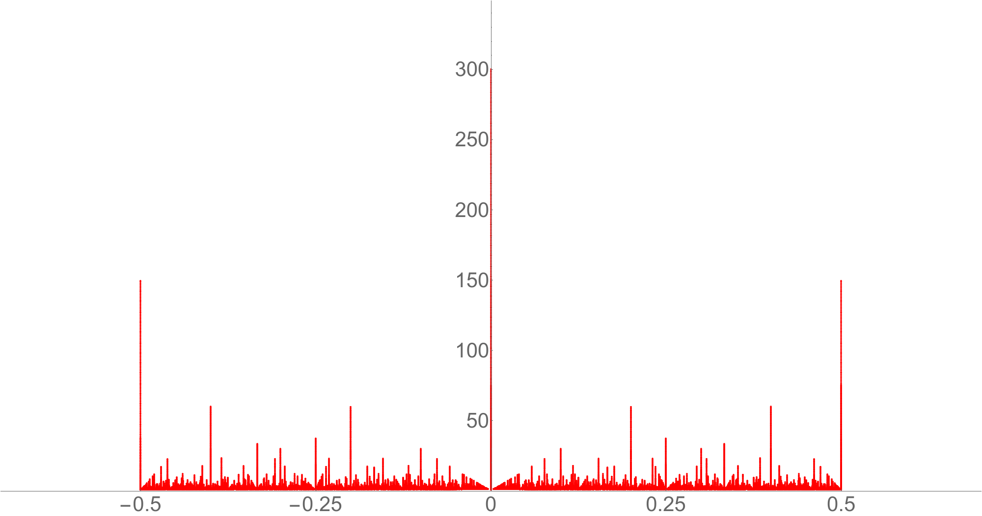
  Figure 1: Space of solutions for the axio-dilaton $\tau$ with fluxes (3.2), mapped to the fundamental domain $\mathcal{F}_{\tau}$. All solutions satisfy the bound $\frac{\mathsf{Q}^{0}}{768}\leq\frac{\mathsf{Q}_{\rm max}^{0}}{768}=300$.

  

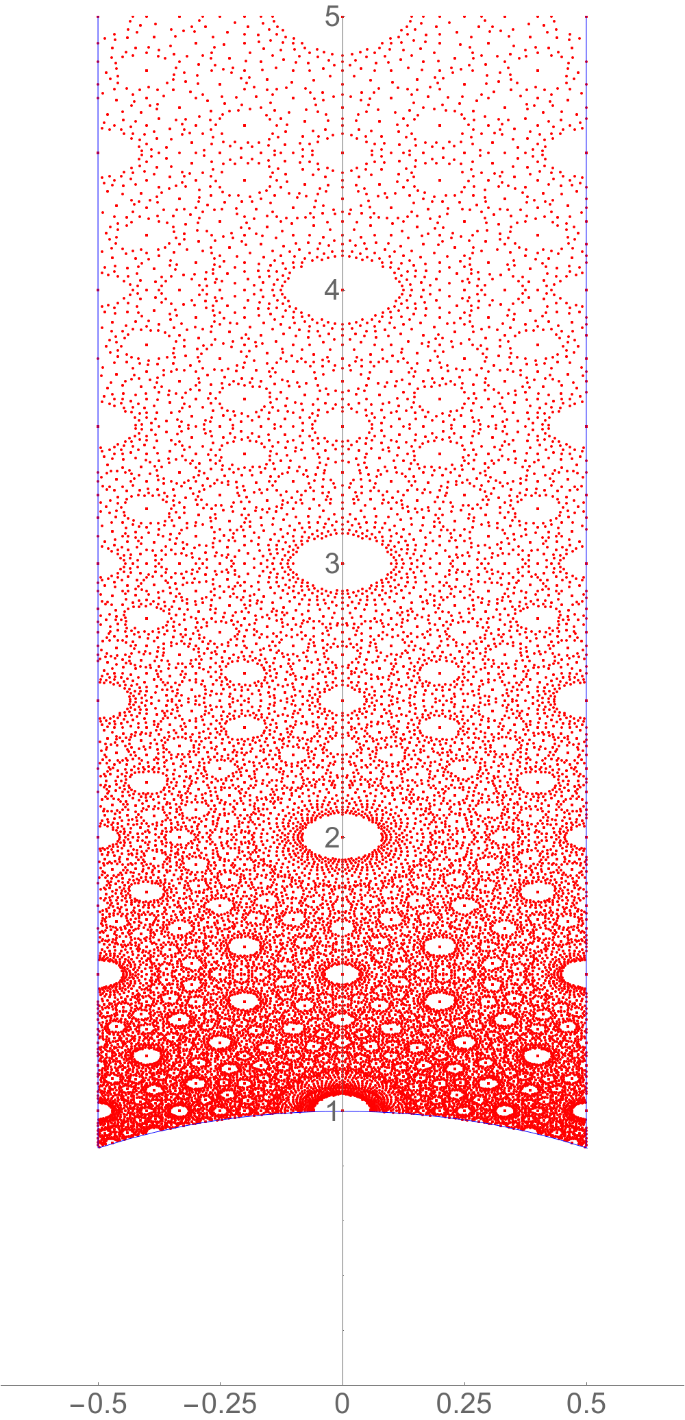
  Figure 2: Zoom of figure 1 for a $0\leq\tau_{2}\leq 5$.

Let us next note that the moduli space of the axio-dilaton $\tau$ is hyperbolic. Indeed from the Kähler potential (2.41) we can derive the corresponding Kähler metric with components

$$\begin{split}\mathcal{G}_{\tau_{1}\tau_{1}}=\mathcal{G}_{\tau_{2}\tau_{2}}=\frac{1}{4{\tau_{2}}^{2}}\,,\hskip 50.0pt\mathcal{G}_{\tau_{1}\tau_{2}}=0\,.\end{split}$$ (3.11)

A convenient way to visualize this hyperbolic space is by mapping the Poincaré half-plane to the Poincaré disk via the conformal transformation

$$\begin{split}\left(\tau_{1},\tau_{2}\right)\to\left(\tilde{\tau}_{1},\tilde{\tau}_{2}\right)=\left(\frac{2\hskip 1.0pt\tau_{1}}{\tau_{1}^{2}+\left(1+\tau_{2}\right)^{2}}\,,\,\frac{\tau_{1}^{2}+\tau_{2}^{2}-1}{\tau_{1}^{2}+\left(1+\tau_{2}\right)^{2}}\right).\end{split}$$ (3.12)

The space of solutions for the axio-dilaton mapped to the Poincaré disk is then shown in figure 3, which is the mapping of figure 1 under (3.12).

• In figure 3 the characteristic structure of voids is visible. In this plot effects of the moduli-space metric are incorporated.

  

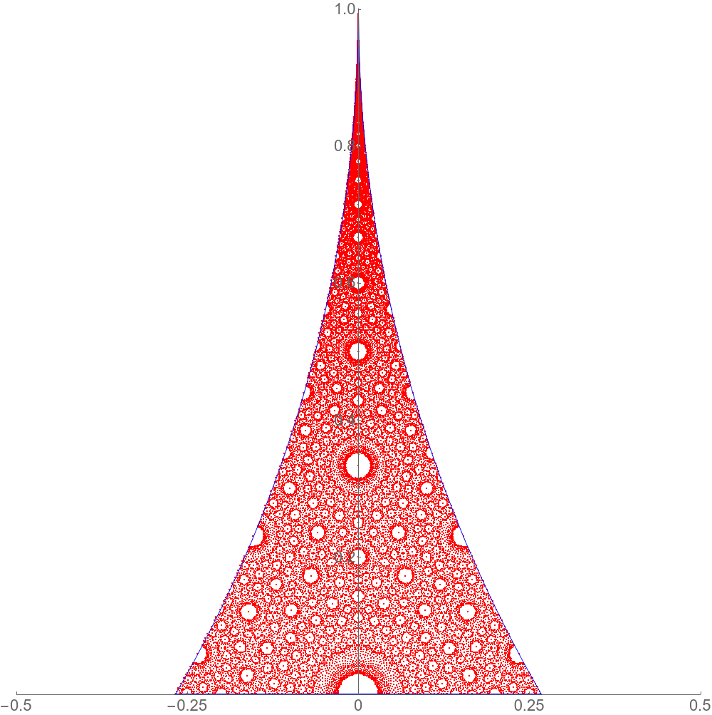
  Figure 3: Space of solutions for the axio-dilaton $\tau$ with fluxes of the form (3.2), restricted to the fundamental domain and mapped to the Poincaré disk. All solutions satisfy the bound $\frac{\mathsf{Q}^{0}}{768}\leq 300$.

  

  Figure 4: Space of solutions for the axio-dilaton $\tau$ with fluxes of the form (3.2) near $\tau=2i$ on the Poincaré plane for $\frac{\mathsf{Q}^{0}}{768}\leq 300$ (blue) and $\frac{\mathsf{Q}^{0}}{768}\leq 3000$ (red).

Analysis of voids

The number of physically-distinct solutions for the axio-dilaton is finite for fixed tadpole-contribution $\mathsf{Q}^{0}$. The number of solutions $\mathsf{N}$ with $\mathsf{Q}^{0}\leq\mathsf{Q}^{0}_{\rm max}$ can be determined numerically, which leads to the following scaling behaviour

$$\begin{split}\mathsf{N}\approx 0.823\left[\frac{\mathsf{Q}_{\rm max}^{0}}{768}\right]^{2}\end{split}$$ (3.13)

for large $\mathsf{Q}_{\rm max}^{0}$. We now want to study how the voids change depending on $\mathsf{N}$, or, equivalently, depending on $\mathsf{Q}^{0}_{\rm max}$. In particular, we are interested how the size of the voids depends on $\mathsf{Q}^{0}_{\rm max}$. Qualitatively, this behaviour is illustrated in figure 4:

• In figure 4 the space of solutions for the axio-dilaton around the point $\tau=2i$ is shown. The blue points correspond to solutions which satisfy $\frac{\mathsf{Q}^{0}}{768}\leq 300$, and the red points correspond to solutions with $\frac{\mathsf{Q}^{0}}{768}\leq 3000$. For larger $\mathsf{Q}^{0}_{\rm max}$ the void around $\tau=2i$ therefore becomes smaller, and finer void structures appear. These results are in agreement with the topological data analysis in [29].

Let us denote the origin of a void by $\tau_{\rm void}$, and define its size by the distance to the nearest solution $\tau_{\rm sol}$ (not located at $\tau_{\rm void}$). The geodesic distance $d$ is measured using the metric (3.11) on the axio-dilaton moduli space, for which we have

$$\begin{split}d\left(\tau\,,\widetilde{\tau}\right)=\frac{1}{2}\hskip 1.0pt\textrm{arccosh}\left[1+\frac{\left(\widetilde{\tau_{1}}-\tau_{1}\right)^{2}+\left(\widetilde{\tau_{2}}-\tau_{2}\right)^{2}}{2\hskip 1.0pt\widetilde{\tau_{2}}\hskip 1.0pt\tau_{2}}\right].\end{split}$$ (3.14)

As we can see for instance from figure 3, in the proper distance the voids can be approximated by a circle whose radius we define as

$$\begin{split}R_{\rm void}=\min_{\tau_{\rm sol}\neq\tau_{\rm void}}d(\tau_{\rm void},\tau_{\rm sol})\,.\end{split}$$ (3.15)

The scaling behaviour of $R_{\rm void}$ with $\mathsf{Q}^{0}_{\rm max}$ has been obtained for instance in [16, 20] as $R^{2}_{\rm void}\sim 1/\mathsf{Q}^{0}_{\rm max}$, and below we have determined the prefactors for some families of voids numerically. For voids located in the fundamental domain on the Poincaré plane we have the following relation between the radius of the void $R_{\rm void}$, the tadpole contribution $\mathsf{Q}^{0}_{\rm max}$ and the number of solutions located at the center of the void $n_{\rm void}$

$$\begin{split}\begin{array}[]{lcl}R_{\rm void}^{2}&\approx&\displaystyle\frac{1}{C\hskip 1.0pt\tau_{2{\rm void}}}\left[\frac{768}{\mathsf{Q}_{\rm max}^{0}}\right]\\[18.0pt] n_{\rm void}&\approx&\displaystyle\frac{2\pi}{C\hskip 1.0pt\tau_{2{\rm void}}}\left[{\frac{\mathsf{Q}_{\rm max}^{0}}{768}}\right]\end{array}\hskip 60.0pt\begin{array}[]{c|c||c}\tau_{1{\rm void}}&\tau_{2{\rm void}}&C\\ \hline\cr\hline\cr 0&n&4\\ 0&n+0.5&16\\ \pm 0.2&n+0.4&20\\ \pm 0.2&n+0.6&20\end{array}\end{split}$$ (3.16)

where $n\in\mathbb{Z}_{+}$. The constant $C$ depends on the family of voids under consideration and can be read-off from the table in (3.16) for several examples. Note also that the number of solutions located at the center of the void divided by the area of the void takes the simple form

$$\begin{split}\frac{n_{\rm void}}{2\pi R_{\rm void}^{2}}\approx\left[\frac{\mathsf{Q}_{\rm max}^{0}}{768}\right]^{2}\,.\end{split}$$ (3.17)

Solutions at small coupling

The imaginary part of the axio-dilaton $\tau$ is bounded from above by the D3-tadpole contribution $\mathsf{Q}^{0}$, which via (2.33) implies a restriction on the string coupling $g_{\rm s}$ as

$$\begin{split}\tau_{2}=e^{-\phi}=\frac{1}{g_{\rm s}}\leq\frac{\mathsf{Q}^{0}}{768}\hskip 40.0pt\Rightarrow\hskip 40.0ptg_{\rm s}\geq\frac{768}{\mathsf{Q}^{0}}\,.\end{split}$$ (3.18)

Recall that in our conventions $\mathsf{Q}^{0}$ is a multiple of $768$. In the following we determine the number of physically-distinct solutions $\mathsf{N}_{\mathsf{c}}$ which satisfy $\tau_{2}\geq\mathsf{c}$ for some cutoff $\mathsf{c}>0$ so that we have

$$\begin{split}\frac{768}{\mathsf{Q}^{0}_{\rm max}}\leq g_{\rm s}\leq\frac{1}{\mathsf{c}}\,.\end{split}$$ (3.19)

Note that in order to ignore string-loop corrections and corrections from world-sheet instantons, we need to stabilize the axio-dilaton at small $g_{\rm s}$. This implies that $\mathsf{Q}^{0}$ and $\mathsf{c}$ should be sufficiently large. Using then the exact data for the space of solutions, we can obtain fits for $\mathsf{N}_{\mathsf{c}}$ for values of $\mathsf{Q}^{0}_{\rm max}$ of the order $\frac{\mathsf{Q}_{\rm max}^{0}}{768}=\mathcal{O}(10^{3})$. In particular, with the scaling of the total number of solutions $\mathsf{N}$ shown in (3.13) we have

$$\begin{split}\frac{\mathsf{Q}^{0}_{\rm max}}{768}\gg 1\hskip 60.0pt\begin{array}[]{c||cc}\mathsf{c}&\mathsf{N}_{\mathsf{c}}&\mathsf{N}_{\mathsf{c}}/\mathsf{N}\\ \hline\cr\hline\cr 2&0.393\bigl{[}\frac{\mathsf{Q}_{\rm max}^{0}}{768}\bigr{]}^{2}&0.478\\ 5&0.157\bigl{[}\frac{\mathsf{Q}_{\rm max}^{0}}{768}\bigr{]}^{2}&0.191\\ 10&0.078\bigl{[}\frac{\mathsf{Q}_{\rm max}^{0}}{768}\bigr{]}^{2}&0.095\\ 20&0.039\bigl{[}\frac{\mathsf{Q}_{\rm max}^{0}}{768}\bigr{]}^{2}&0.047\end{array}\end{split}$$ (3.20)

We observe that in this limit the percentage of solutions with $g_{\rm s}\ll 1$ is small and independent of $\mathsf{Q}^{0}_{\rm max}$. For instance, only about 5% of the solutions have a string coupling satisfying $g_{\rm s}\leq 0.05$.

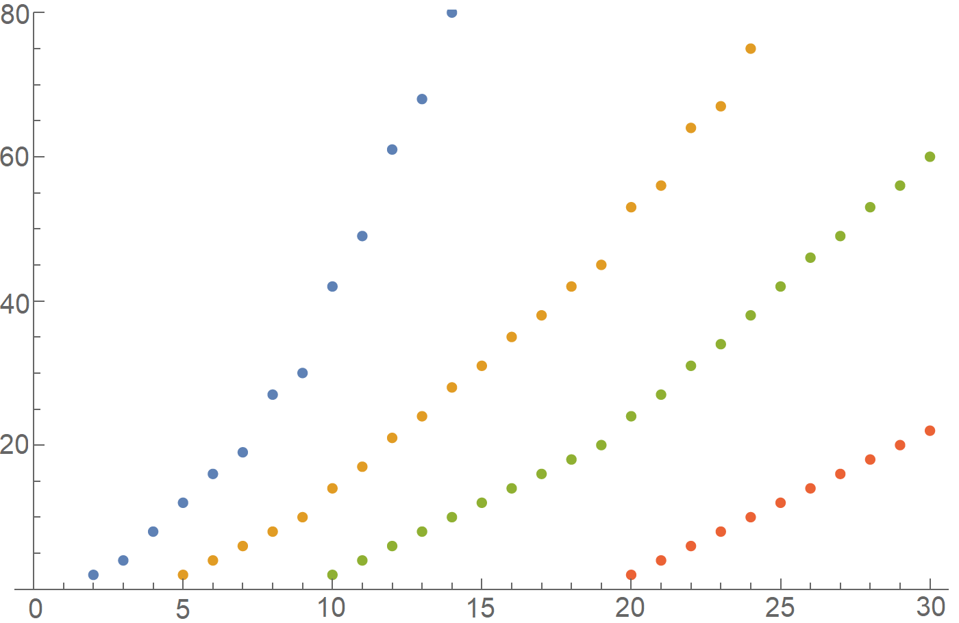
Figure 5: Number of solutions $\mathsf{N}_{\mathsf{c}}$ (for the axio-dilaton $\tau$ with fluxes of the form (3.2)) which satisfy $\mathsf{c}\leq\tau_{2}\leq\frac{\mathsf{Q}_{\rm max}^{0}}{768}$ for $\mathsf{c}=2,5,10,20$ in colors blue, orange, green and red, respectively.

However, the region of small tadpole contributions $\frac{\mathsf{Q}^{0}}{768}=\mathcal{O}(1)$ is more interesting. Here the number of solutions $\mathsf{N}_{\mathsf{c}}$ does not follow a simple quadratic behavior, and the precise numbers are shown in figure 5. We see that for a particular $\mathsf{c}$ in $g_{\rm s}\leq 1/\mathsf{c}$, the D3-tadpole contributions $\frac{\mathsf{Q}^{0}}{768}$ has to be larger than some threshold. Furthermore, above this threshold the number of solutions is not large but only $\mathcal{O}(10)$.

3.4 Summary

Let us summarize the results and observations of this section for moduli stabilization of the axio-dilaton with the choice of fluxes given in equation (3.4):

• As already known before, for a fixed D3-brane tadpole contribution $\mathsf{Q}^{0}$, the number of physically-distinct solutions to the F-term equations for the axio-dilaton $\tau$ is finite due to the corresponding $SL(2,\mathbb{Z})$ duality [16, 20].

• The solutions for the axio-dilaton in the fundamental domain are not distributed homogeneously, but show characteristic void structures as illustrated in figures 2 and 3.

• With increasing upper bound $\mathsf{Q}^{0}_{\rm max}$ on the tadpole contribution, the area of these voids shrinks and the number of solutions located at the center $n_{\rm void}$ increases as shown in (3.16). The precise behaviour for the radius $R_{\rm void}$ and $n_{\rm void}$ is proportional to a constant depending on the location of the void, however, the ratio $n_{\rm void}/2\pi R_{\rm void}^{2}$ is universal.

• The string coupling is bounded from below by the tadpole contribution as $\frac{768}{\mathsf{Q}^{0}}\leq g_{\rm s}$. In order to ignore string corrections and trust the solutions (3.4), we have to demand $g_{\rm s}\ll 1$ which implies $\frac{\mathsf{Q}^{0}}{768}\gg 1$. This is in contrast to our discussion of the tadpole-cancellation condition on page 2.2 which requires $\frac{\mathsf{Q}^{0}}{768}$ to be small, and illustrates the difficulty of obtaining reliable solutions to the F-term equations.

• We have furthermore analyzed the number of physically-distinct solutions satisfying $g_{\rm s}\leq 1/\mathsf{c}$. Requiring a small string coupling of for instance $g_{\rm s}\leq 1/10$, we find that only about $10\%$ of the solutions satisfy this condition. If we require $g_{\rm s}$ to be smaller, then the corresponding fraction of solutions is smaller.

4 Moduli stabilization II

In this section we extend our previous discussion by including the complex-structure moduli $U^{i}$. We choose flux configurations which stabilize the axio-dilaton and fix the complex-structure moduli at an isotropic minimum with $U^{1}=U^{2}=U^{3}$. Such vacua have previously been studied for instance in [60, 20].

4.1 Setting

We start again by specifying the superpotential (2.42) and set to zero the non-geometric fluxes (2.35)

$$\begin{split}q_{I}{}^{\mathsf{A}}=0\,,\hskip 40.0ptq^{I\mathsf{A}}=0\,,\end{split}$$ (4.1)

and for the R-R and remaining NS-NS fluxes (2.34) we choose the following restricted setting

$$\begin{split}\begin{array}[]{lclcl@{\hspace{40pt}}lclcl}f_{1}&=&f_{2}&=&f_{3}\,,\hfil\hskip 40.&h_{1}&=&h_{2}&=&h_{3}\,,\\[6.0pt] f^{1}&=&f^{2}&=&f^{3}\,,\hfil\hskip 40.&h^{1}&=&h^{2}&=&h^{3}\,,\end{array}\hskip 40.0ptf^{I},f_{I},h^{I},h_{I}\in 8\mathbb{Z}\,.\end{split}$$ (4.2)

Since the superpotential is independent of the Kähler moduli $T_{\mathsf{A}}$, the F-term equations (2.46) simplify as in (3.3) and we obtain

$$\begin{split}0=W\,,\hskip 40.0pt0=\partial_{U^{i}}W\,,\hskip 40.0pt0=\partial_{\tau}W\,.\end{split}$$ (4.3)

Due to the isotropic choice of fluxes in (4.2), the complex-structure moduli $U^{i}$ are stabilized such that

$$\begin{split}U^{1}=U^{2}=U^{3}=:U\,,\end{split}$$ (4.4)

and the F-term equations (4.3) reduce to

$$\begin{array}[]{lcl@{\op}lcl@{\op}lcl@{\op}lcl@{}}-f_{0}&-&3\hskip 1.0ptU\hfil\hskip 1.0pt&f_{1}&-&3\hskip 1.0pt(U)^{2}\hfil\hskip 1.0pt&f^{1}&+&(U)^{3}\hfil\hskip 1.0pt&f^{0}&=&0\,,\\[4.0pt] -h_{0}&-&3\hskip 1.0ptU\hfil\hskip 1.0pt&h_{1}&-&3\hskip 1.0pt(U)^{2}\hfil\hskip 1.0pt&h^{1}&+&(U)^{3}\hfil\hskip 1.0pt&h^{0}&=&0\,,\end{array}$$ (4.7)

$$(f_{1}-\tau h_{1})+2\hskip 1.0ptU(f^{1}-\tau h^{1})-(U)^{2}(f^{0}-\tau h^{0})=0\,.$$ (4.8)

The R-R and NS-NS fluxes in (4.2) are furthermore subject to the Bianchi identities (2.38), and due to the vanishing $Q$-fluxes the only nontrivial relation is again given by the D$3$-brane tadpole contribution

$$\begin{split}\mathsf{Q}^{0}=f_{0}\hskip 1.0pth^{0}-f^{0}\hskip 1.0pth_{0}+3\left(f_{1}\hskip 1.0pth^{1}-f^{1}\hskip 1.0pth_{1}\right)>0\,.\end{split}$$ (4.9)

Note that due to the quantization condition for the fluxes, the tadpole contribution $\mathsf{Q}^{0}$ is an integer multiple of $64$. However, as it has been explained in footnote 10 of [60], in order to obtain physically-viable solutions $\mathsf{Q}^{0}$ receives an additional factor of three. The tadpole contribution is therefore always a multiple of $192$, which is also what we see explicitly in our data.

4.2 Finite number of solutions for fixed $\mathsf{Q}^{0}$

The two equations for the complex-structure modulus shown in (4.7) define an overdetermined cubic system for $U$, which in general does not allow for a solution in closed form. Since the coefficients in (4.7) are real, one can bring these equations into the form

$$\begin{split}(U-u_{0})\hskip 1.0pt(U-u_{1})\hskip 1.0pt(U-\bar{u}_{1})=0\,,\hskip 40.0ptu_{0}\in\mathbb{R}\,,\;u_{1}\in\mathbb{C}\,,\end{split}$$ (4.10)

where $u_{0},u_{1},\bar{u}_{1}$ denote the solutions. Physically-acceptable solutions have to satisfy $\mbox{Im}\hskip 1.0ptU>0$, and therefore the F-term equations (4.7) have at most one solution for $U$ of interest to us. The equation (4.8) can be solved for the axio-dilaton as

$$\begin{split}\tau=\frac{f_{1}+2\hskip 1.0ptUf^{1}-(U)^{2}\hskip 1.0ptf^{0}}{h_{1}+2\hskip 1.0ptUh^{1}-(U)^{2}\hskip 1.0pth^{0}}\,,\end{split}$$ (4.11)

which however depends on $U$. More details on these solutions can be found in appendix A, where we follow the discussion of [60, 20]. As reviewed in section 2.4, in the absence of non-geometric $Q$-fluxes the axio-dilaton and the complex-structure moduli enjoy $SL(2,\mathbb{Z})$ dualities. These can be used to bring $\tau$ and $U$ into their fundamental domains

$$\begin{split}\begin{array}[]{lclclrlclllrcl}\mathcal{F}_{\tau}&=&\displaystyle\biggl{\{}-\frac{1}{2}\leq&\tau_{1}&\leq 0,&|\tau|^{2}&\geq 1&\cup&\;0<&\tau_{1}&\displaystyle<+\frac{1}{2},&|\tau|^{2}&>&1\biggr{\}}\,,\\[14.0pt] \mathcal{F}_{U}&=&\displaystyle\biggl{\{}-\frac{1}{2}\leq&U_{1}&\leq 0,&|U|^{2}&\geq 1&\cup&\;0<&U_{1}&\displaystyle<+\frac{1}{2},&|U|^{2}&>&1\biggr{\}}\,,\end{array}\end{split}$$ (4.12)

where we again split $\tau$ and $U$ into their real and imaginary parts as $\tau=\tau_{1}+i\hskip 1.0pt\tau_{2}$ and $U=U_{1}+i\hskip 1.0ptU_{2}$. We furthermore note that the two $SL(2,\mathbb{Z})$ dualities leave the D3-tadpole contribution $\mathsf{Q}^{0}$ invariant. Now, as shown by [60, 20] and reviewed in appendix A, the dualities can be used to show that the number of physically-distinct vacua in the fundamental domain is finite for fixed $\mathsf{Q}^{0}$. In the following we explore how the properties of the space of solutions for $\tau$ and $U$ depend on $\mathsf{Q}^{0}$.

4.3 Space of solutions

In this section we study the space of solutions to the F-term equations (2.46) for the combined axio-dilaton and complex-structure-modulus system. Since for the axio-dilaton system we found two-dimensional circular voids in the two-dimensional moduli space, it is natural to expect four-dimensional spherical voids in the four-dimensional moduli space. However, we can not confirm this expectation. Our data has again been obtained using a computer algorithm, which generated all physically-distinct flux vacua for a given upper bound on the D3-brane tadpole contribution $\mathsf{Q}^{0}$.

Distribution of solutions

In [60, 20] (as well as in appendix A) it is shown that for fixed $\mathsf{Q}^{0}$ the number of physically-distinct solutions is finite. We have determined all solutions for the setting described in section 4.1 numerically, and have visualized them in the following figures.

• In figure 6 we have shown the solutions for the fluxes of the form (4.2) projected onto the $\tau$ and onto the $U$-plane [20]. All solutions satisfy the bound on the tadpole contribution $\frac{\mathsf{Q}^{0}}{192}\leq 1000$, and in order to have a symmetric plot we included points on the boundary of the fundamental domains. These plots are similar to the one in figure 1. When comparing figures 6(a) and 6(b), we note that for the same $\mathsf{Q}^{0}$ the maximum values for $\tau_{2}$ and $U_{2}$ differ significantly. Furthermore, we note that the number of different values for $\tau_{1}$ is much larger than for $U_{1}$.

  

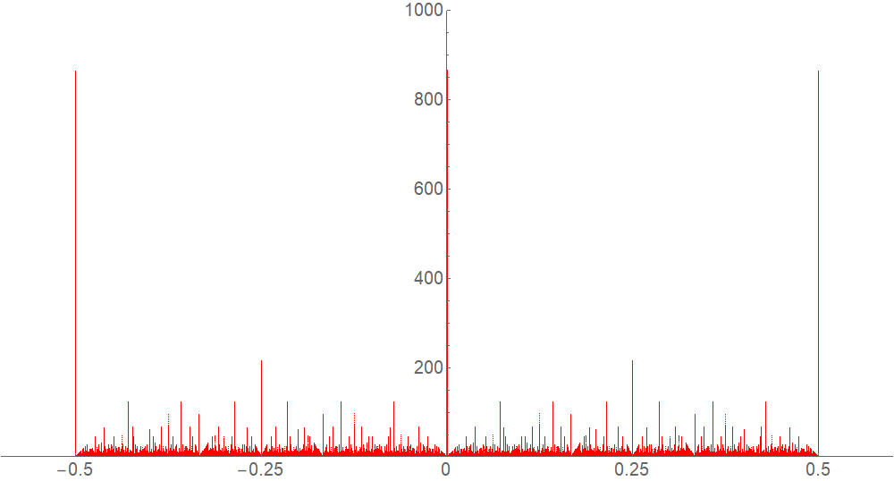
  (a) Projection of solutions onto the $\tau$-plane.

  

  (b) Projection of solutions onto the $U$-plane.

  Figure 6: Space of solutions for the setting described in section 4.1, mapped to the fundamental domains $\mathcal{F}_{\tau}$ and $\mathcal{F}_{U}$ and projected onto the $\tau$- and $U$-plane. All solutions satisfy the bound $\frac{\mathsf{Q}^{0}}{192}\leq 1000$.

• In figure 7 we show sections through the four-dimensional space of solutions for $\tau_{2}\leq 2$, characterized by different values of the complex-structure modulus. All solutions satisfy $\frac{\mathsf{Q}^{0}}{192}\leq 1000$, and these plots show void structures similar as in figure 2. We note however that although the location of the voids stays the same when going from $U=i$ to $U=2i$ and similarly from $U=\sqrt{2}i$ to $U=2\sqrt{2}i$, the density of solutions decreases. This appears to be a general feature which we observe in the data.

  

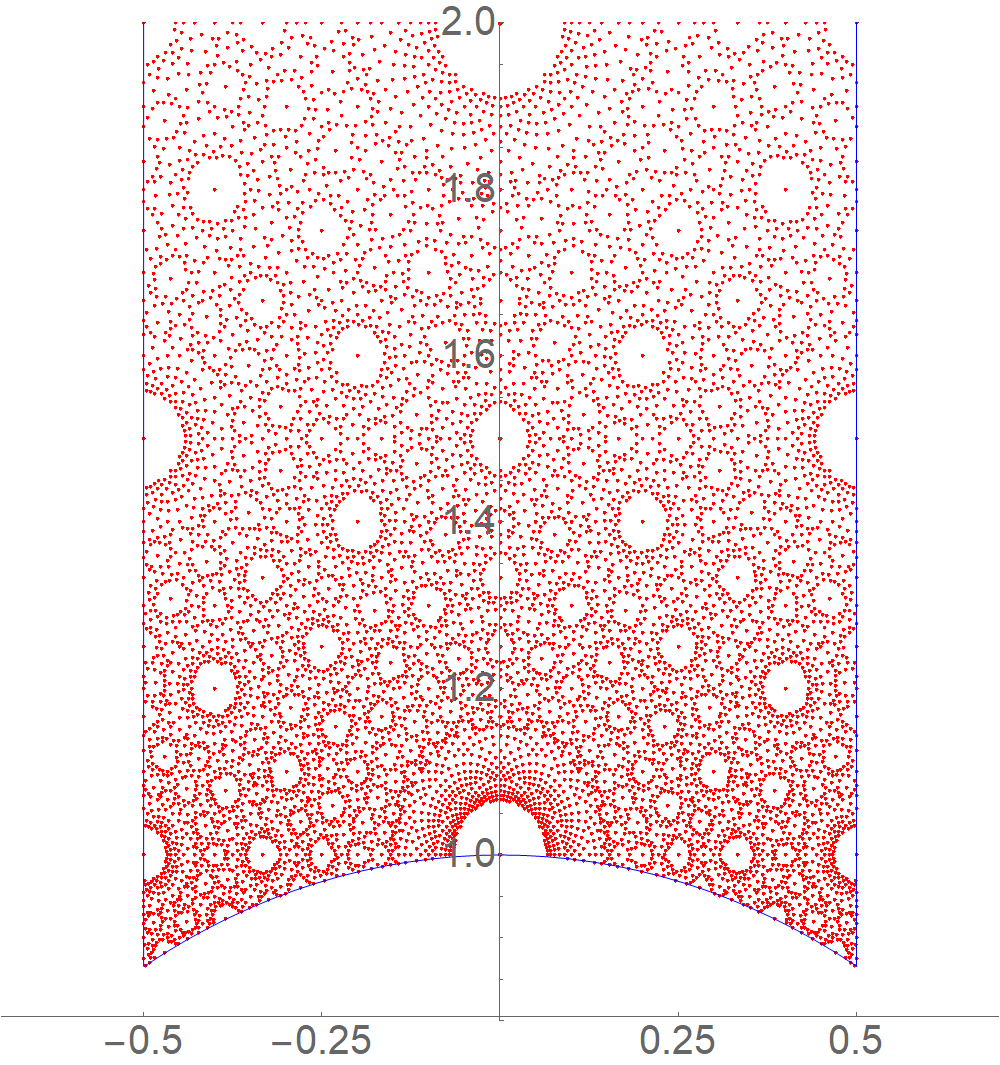
  (a) $U=i$

  

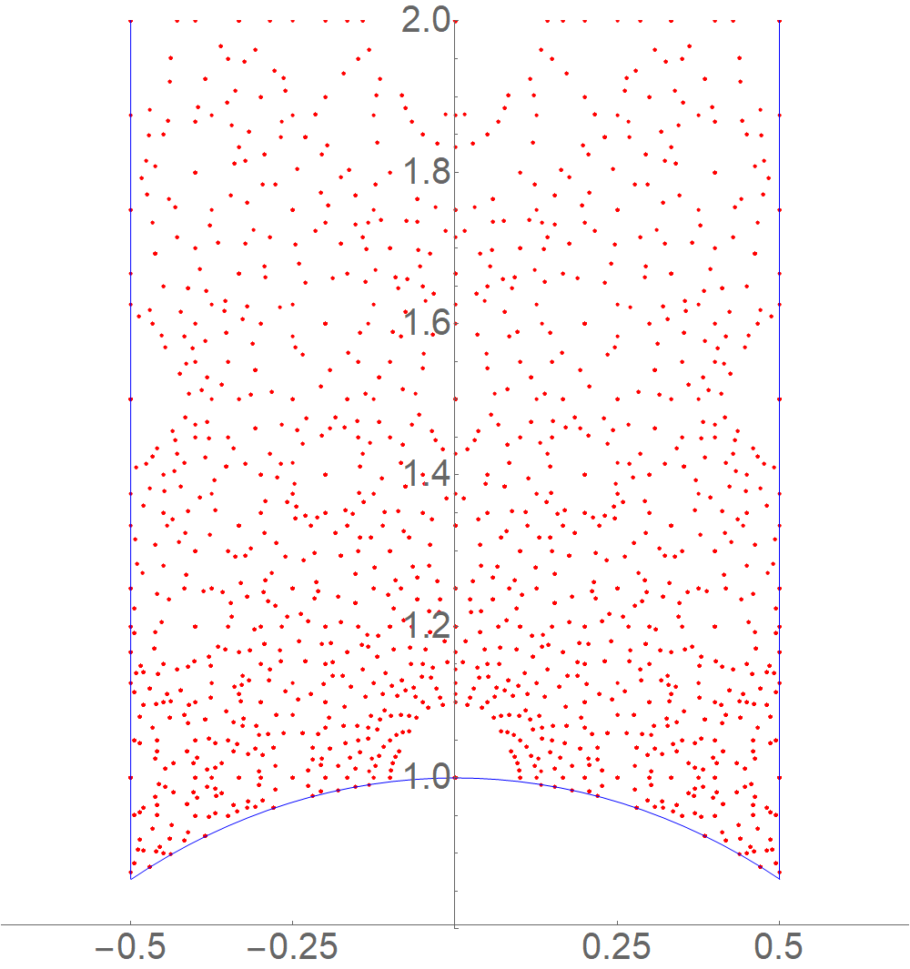
  (b) $U=2i$

  

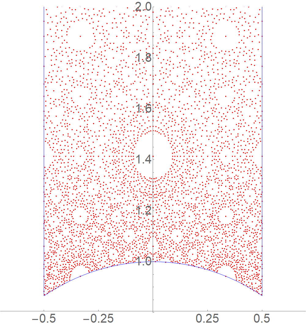
  (c) $U=\sqrt{2}i$

  

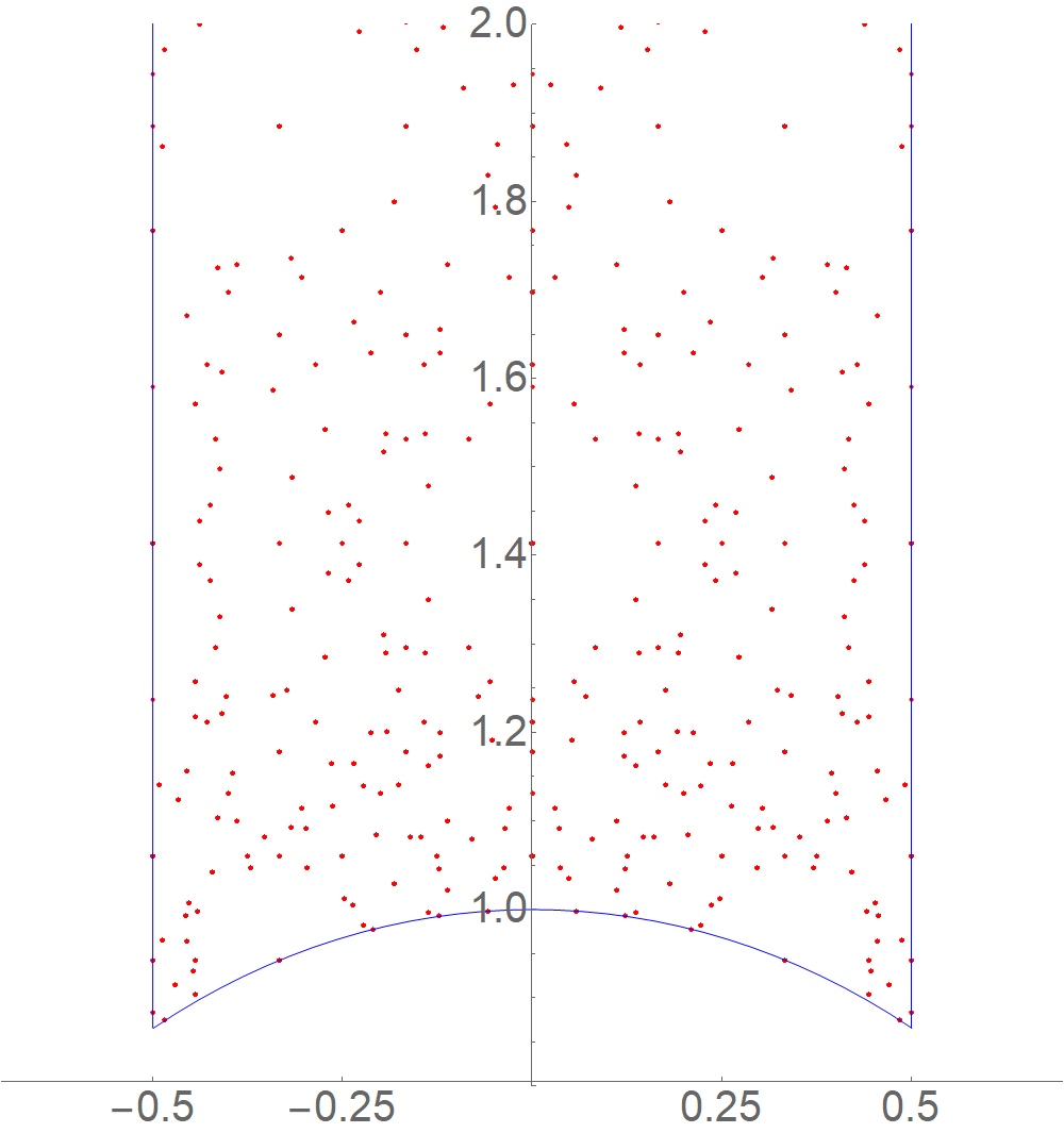
  (d) $U=2\sqrt{2}i$

  Figure 7: Section through the four-dimensional space of solutions for the setting described in section 4.1. The solutions have been mapped to the fundamental domains, and the sections are for fixed complex-structure modulus at $U=i$, $U=2i$, $U=\sqrt{2}i$ and $U=2\sqrt{2}i$. All solutions satisfy the bound $\frac{\mathsf{Q}^{0}}{192}\leq 1000$.

• In figure 8 we have shown three-dimensional sections of the four-dimensional space of solutions for $U_{1}=0$. All solutions have been mapped to the fundamental domain. Figures 8(a) and 8(b) show two different points of view, which illustrate that the three-dimensional section of the space of solutions is not homogenous. Solutions are accumulated on planes for particular values of $U_{2}$, while the space between these planes is only sparsely populated. This is in agreement with our observations in figures 7, which also show that the density of solutions varies.

  The lines in figures 8(a) and 8(b) connect voids for different values of $U_{2}$ and are described by the following equations for $t\in\mathbb{R}_{+}$

  $$\begin{split}\begin{array}[]{l@{\hspace{15pt}}l@{\hspace{30pt}}lcl@{\op}r@{\op}r@{\op}l@{\op}l@{\op}l}\mbox{orange}\hfil\hskip 15.0&l_{1}\hfil\hskip 30.&(\tau_{1},\tau_{2},U_{1},U_{2})&=&(\hfil\hskip 1.0pt&0\hskip 1.0pt&,\,1+t\hskip 1.0pt&,\,0\hfil\hskip 1.0pt&,\,1+\frac{1}{1}\hskip 1.0ptt\hfil\hskip 1.0pt&)\,,\\[4.0pt] \mbox{red}\hfil\hskip 15.0&l_{2}\hfil\hskip 30.&(\tau_{1},\tau_{2},U_{1},U_{2})&=&(\hfil\hskip 1.0pt&0\hskip 1.0pt&,\,2+t\hskip 1.0pt&,\,0\hfil\hskip 1.0pt&,\,1+\frac{1}{2}\hskip 1.0ptt\hfil\hskip 1.0pt&)\,,\\[4.0pt] \mbox{purple}\hfil\hskip 15.0&l_{3}\hfil\hskip 30.&(\tau_{1},\tau_{2},U_{1},U_{2})&=&(\hfil\hskip 1.0pt&0\hskip 1.0pt&,\,3+t\hskip 1.0pt&,\,0\hfil\hskip 1.0pt&,\,1+\frac{1}{3}\hskip 1.0ptt\hfil\hskip 1.0pt&)\,,\\[4.0pt] \mbox{green}\hfil\hskip 15.0&l_{4}\hfil\hskip 30.&(\tau_{1},\tau_{2},U_{1},U_{2})&=&(\hfil\hskip 1.0pt&-\frac{1}{2}\hskip 1.0pt&,\,\frac{3}{2}+t\hskip 1.0pt&,\,0\hfil\hskip 1.0pt&,\,1+\frac{2}{3}\hskip 1.0ptt\hfil\hskip 1.0pt&)\,.\end{array}\end{split}$$ (4.13)

  

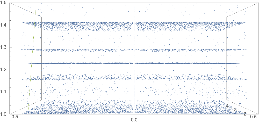
  (a) Point of view along the $\tau_{2}$-direction.

  

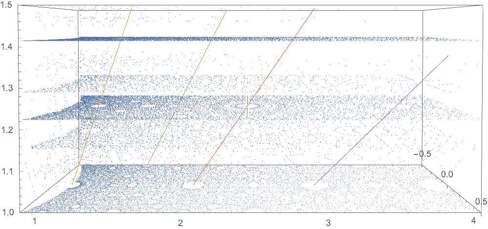
  (b) Point of view along the $\tau_{1}$-direction.

  Figure 8: Section through the four-dimensional space of solutions with $U_{1}=0$ for the setting described in section 4.1. All solutions satisfy the bound $\frac{\mathsf{Q}^{0}}{192}\leq 1000$ and have been mapped to the fundamental domains. The lines in 8(a) and 8(b) connect voids for different values of $U_{2}$ and are described by the expressions in equation (4.13).

• In figure 9 we have shown the same three-dimensional section of the space of solutions as in figure 8. The point of view in figure 9(a) is along the line $l_{1}$ (orange) of (4.13) and the point of view in figure 9(b) is along the line $l_{2}$ (red). In these three-dimensional sections of the four-dimensional space of solutions we therefore have a cylindrical void centered around the lines in (4.13).

  

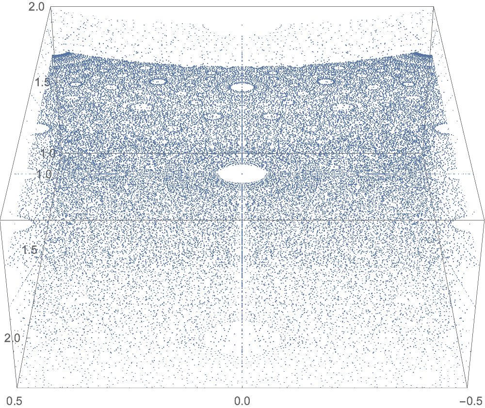
  (a) View along the line $l_{1}$ (orange) in figures 8.

  

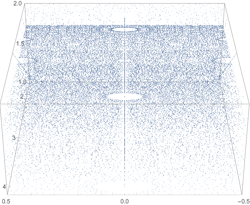
  (b) View along the line $l_{2}$ (red) in figures 8.

  Figure 9: Section through the four-dimensional space of solutions with $U_{1}=0$ for the setting described in section 4.1. All solutions satisfy the bound $\frac{\mathsf{Q}^{0}}{192}\leq 1000$ and have been mapped to the fundamental domains. The points of view are along the line $l_{1}$ (figure 9(a)) and line $l_{2}$ (figure 9(b)) in figures 8, which show a void structure around $l_{1}$ and $l_{2}$.

Solutions at small coupling and large complex structure

We now consider the number $\mathsf{N}$ of physically-distinct solutions for the combined axio-dilaton and complex-structure moduli system defined in section 4.1. This number is finite for fixed D3-tadpole contribution $\mathsf{Q}^{0}$, and since we have the numerical data we can determine this number explicitly. For large $\mathsf{Q}^{0}$ the dependence takes the form

$$\begin{split}\mathsf{N}\approx 1.2501\left[\frac{\mathsf{Q}^{0}}{192}\right]^{2}.\end{split}$$ (4.14)

We next note that in the fundamental domains, the imaginary parts of the axio-dilaton and complex-structure moduli satisfy a lower bound similarly as in the previous example. An upper bound can be obtained from the numerical data, which can be expressed as 

$$\begin{split}\frac{\sqrt{3}}{2}\leq\tau_{2}\leq\frac{\sqrt{3}}{2}\left[\frac{\mathsf{Q}^{0}}{192}\right],\hskip 80.0pt\frac{\sqrt{3}}{2}\leq U_{2}\leq\frac{\sqrt{3}}{2}\left[\frac{\mathsf{Q}^{0}}{192}\right]^{1/2}.\end{split}$$ (4.15)

Note that in our conventions the tadpole contribution $\mathsf{Q}^{0}$ is a multiple of $192$. However, as we have seen in (4.11), the solution for the axio-dilaton depends on the complex-structure modulus. Although this dependence is difficult to analyze analytically, the numerical data gives the following bound on the solutions

$$\begin{split}\tau_{2}\,U_{2}\leq\frac{3}{4}\hskip 1.0pt\frac{\mathsf{Q}^{0}}{192}\,.\end{split}$$ (4.16)

This bound is stronger than in (4.15), and it implies that for fixed $\mathsf{Q}^{0}$ the imaginary parts of $\tau$ and $U$ cannot be made simultaneously large. In particular, in order to have solutions at small coupling $g_{\rm s}=\frac{1}{\tau_{2}}\ll 1$ and large complex structure $U_{2}\gg 1$, the tadpole contribution has to be sufficiently large. Let us make this more precise and determine numerically the number of solutions $\mathsf{N}_{\mathsf{c}}$ with $\mathsf{Q}^{0}\leq\mathsf{Q}^{0}_{\rm max}$ for which

$$\begin{split}g_{\rm s}\leq\frac{1}{\mathsf{c}}\hskip 50.0pt\mbox{and}\hskip 50.0ptU_{2}\geq\mathsf{c}\,.\end{split}$$ (4.17)

In the limit of large $\frac{\mathsf{Q}_{\rm max}^{0}}{192}$ we obtained the following approximations

$$\begin{split}\frac{\mathsf{Q}^{0}_{\rm max}}{192}\gg 1\hskip 40.0pt\begin{array}[]{c||r@{\hspace{2pt}}rc}\mathsf{c}&\lx@intercol\hfil\mathsf{N}_{\mathsf{c}}\hfil\lx@intercol&\mathsf{N}_{\mathsf{c}}/\mathsf{N}\\ \hline\cr\hline\cr 2&0.0553\bigl{[}\frac{\mathsf{Q}_{\rm max}^{0}}{192}\bigr{]}^{2}\hskip 2.0&-3.4617\bigl{[}\frac{\mathsf{Q}_{\rm max}^{0}}{192}\bigr{]}&0.041\\ 5&0.0047\bigl{[}\frac{\mathsf{Q}_{\rm max}^{0}}{192}\bigr{]}^{2}\hskip 2.0&-0.7627\bigl{[}\frac{\mathsf{Q}_{\rm max}^{0}}{192}\bigr{]}&0.004\\ 10&0.0009\bigl{[}\frac{\mathsf{Q}_{\rm max}^{0}}{192}\bigr{]}^{2}\hskip 2.0&-0.3569\bigl{[}\frac{\mathsf{Q}_{\rm max}^{0}}{192}\bigr{]}&0.001\end{array}\end{split}$$ (4.18)

These approximations do not describe the data very well, but are sufficient for our purposes here. In particular, we see that at leading order $\mathsf{N}_{\mathsf{c}}$ depends quadratically on $\mathsf{Q}^{0}_{\rm max}$ and that the ratios $\mathsf{N}_{\mathsf{c}}/\mathsf{N}$ are rather small. Thus, only a small percentage of the solutions to the F-term equations are in a perturbatively-controlled regime. More interesting is the limit of small $\frac{\mathsf{Q}^{0}}{192}$, which we have illustrated in figure 10. We see that for $\mathsf{c}=2$ (blue) there are solutions starting at $\frac{\mathsf{Q}^{0}}{192}=16$. For $\mathsf{c}=5$ (orange) we find solutions starting at $\frac{\mathsf{Q}^{0}}{192}=100$, and for $\mathsf{c}=10$ (green) solutions can be obtained starting at $\frac{\mathsf{Q}^{0}}{192}=400$.

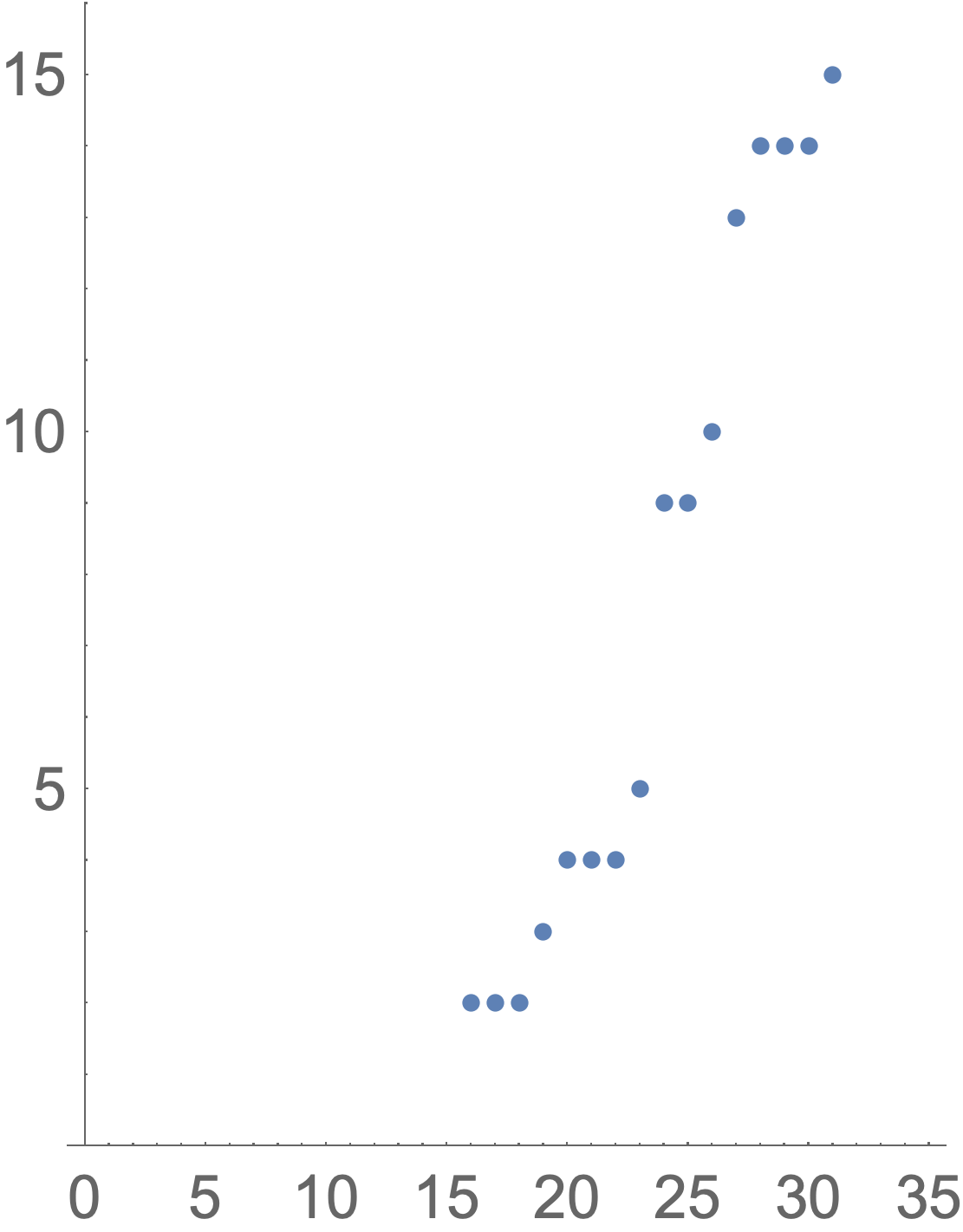
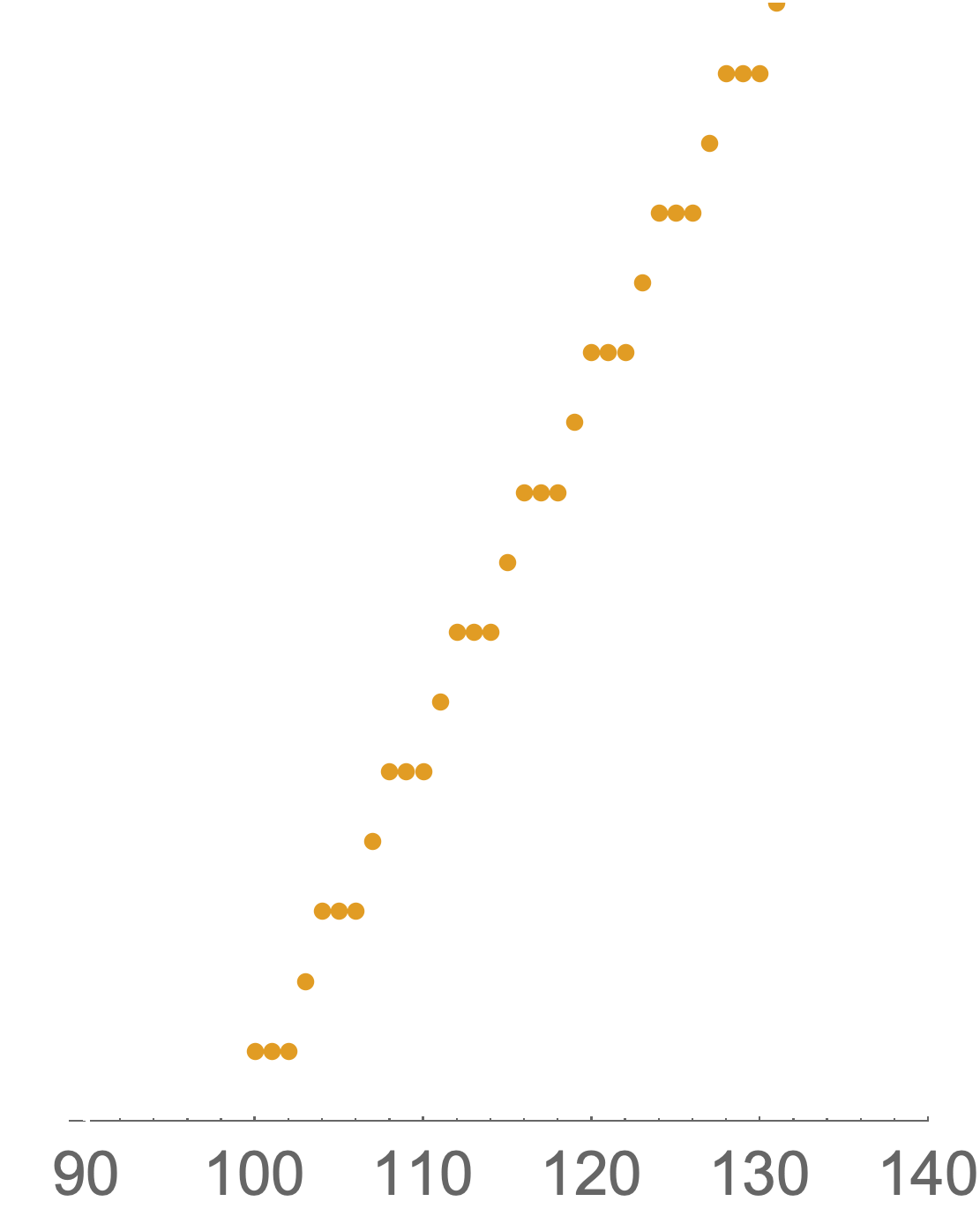
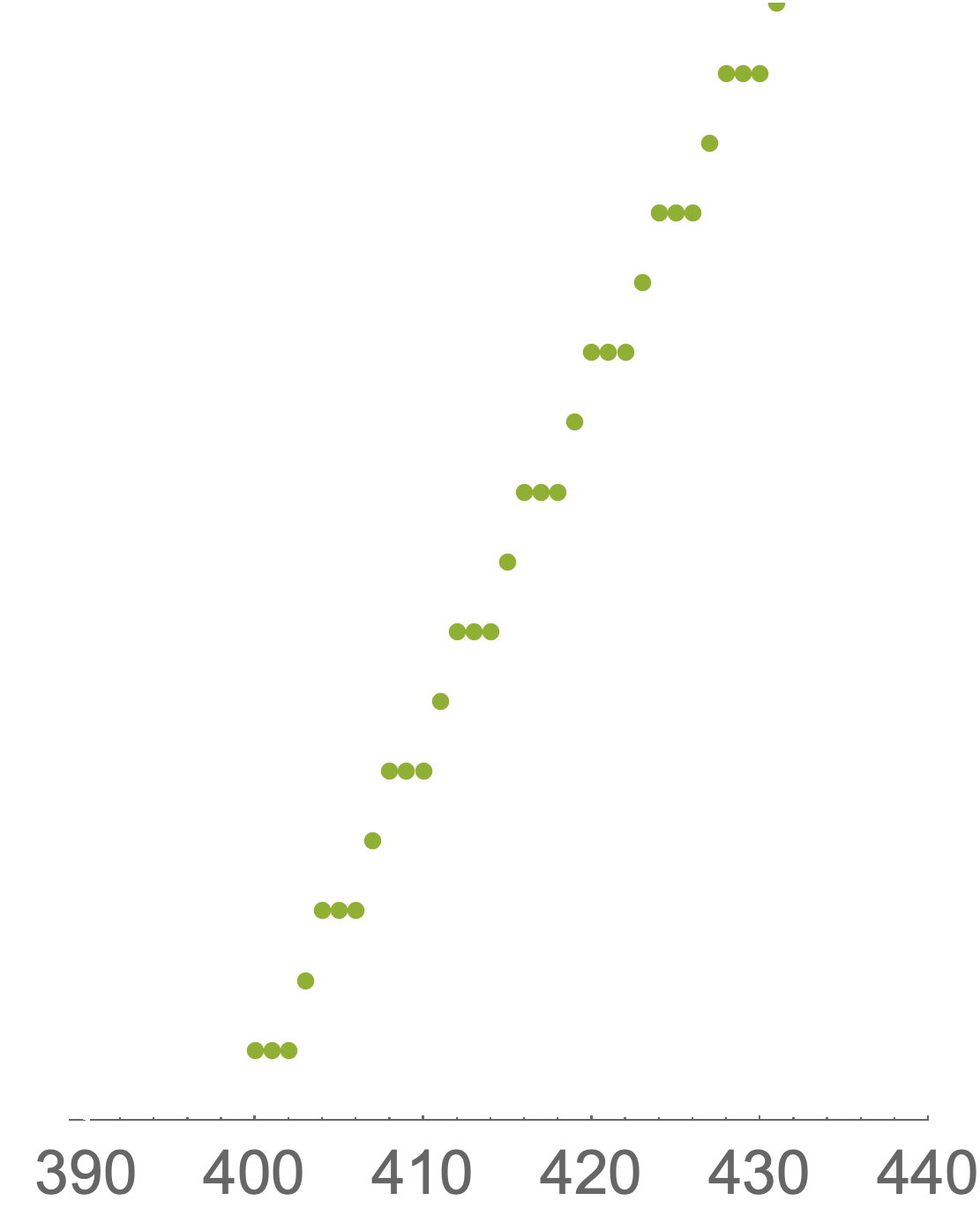
Figure 10: Number of solutions $\mathsf{N}_{\mathsf{c}}$ as a function of $\frac{\mathsf{Q}_{\rm max}^{0}}{192}$ (for the setting described in section 4.1) which satisfy $\tau_{2},U_{2}\geq\mathsf{c}$ for $\mathsf{c}=2,5,10$ in colors blue, orange and green, respectively. Note that different ranges for $\frac{\mathsf{Q}_{\rm max}^{0}}{192}$ on the horizontal axis.

The main conclusion we want to draw from this analysis is that for solutions at weak coupling $g_{\rm s}\ll 1$ and large complex structure $U_{2}\gg 1$, the D3-tadpole contribution $\frac{\mathsf{Q}^{0}}{192}$ has to be large. As discussed on page 2.2, this is in tension with the tadpole cancellation condition.

4.4 Summary

Let us summarize the results obtained in this section for the space of solutions of the combined axio-dilaton and complex-structure-moduli system with fluxes characterized by the setting described in section 4.1:

• As known before, for a fixed D3-brane tadpole contribution $\mathsf{Q}^{0}$ the number of physically-distinct solutions to the F-term equations (2.46) for the axio-dilaton and complex-structure moduli is finite. This is again due to the $SL(2,\mathbb{Z})$ dualities for the axio-dilaton and the complex-structure moduli.

• The values of the fixed moduli (mapped to their fundamental domains) are not distributed homogeneously in the space of solutions. As shown in figures 9, the solutions are accumulated on submanifolds in the four-dimensional space with few points in between. We also find void structures in the space of solutions, which are however not spherical but take a cylindrical form in three-dimensional sections (cf. figures 9).

• The imaginary parts of the axio-dilaton and the complex-structure moduli $\tau_{2}$ and $U_{2}$ are bounded from above and below as shown in equation (4.15). In our data we find however the stronger bound on the product $\tau_{2}\,U_{2}\leq\frac{3}{4}\hskip 1.0pt\frac{\mathsf{Q}^{0}}{192}$, which implies that in the weak-coupling and large-complex-structure regime the tadpole contribution $\frac{\mathsf{Q}^{0}}{192}$ has to be large. This is again in contrast to our arguments regarding the tadpole-cancellation condition on page 2.2 which requires $\frac{\mathsf{Q}^{0}}{192}$ to be small, and illustrates the tension between the closed- and open-string sectors for obtaining reliable solutions.

• We have furthermore shown that the fraction of reliable flux solutions within all solutions for fixed tadpole $\frac{\mathsf{Q}^{0}}{192}$ is only of orders $\mathcal{O}(10^{-3})$, which is a reduction as compared to the setting of section 3.

5 Moduli stabilization III

We now generalize the setting from section 4 by including non-geometric $Q$-fluxes. The fluxes are restricted such that the complex-structure and Kähler moduli are fixed isotropically as $T_{1}=T_{2}=T_{3}:=T$ and $U^{1}=U^{2}=U^{3}:=U$, which reduces the system to the three complex moduli fields $\tau$, $U$ and $T$. Such vacua have previously been analyzed for instance in [23].

5.1 Setting

We specify the superpotential (2.42) by imposing the following restrictions on the R-R and NS-NS fluxes (2.34) and (2.35)

$$\begin{split}\begin{array}[]{lclcl@{\hspace{50pt}}clclclcllclcl}f^{1}&=&f^{2}&=&f^{3}\,,\hfil\hskip 50.&h^{1}&=&h^{2}&=&h^{3}\,,\\ f_{1}&=&f_{2}&=&f_{3}\,,\hfil\hskip 50.&h_{1}&=&h_{2}&=&h_{3}\,,\\[6.0pt] q^{01}&=&q^{02}&=&q^{03}\,,\hfil\hskip 50.\\ q_{0}{}^{1}&=&q_{0}{}^{2}&=&q_{0}{}^{3}\,,\hfil\hskip 50.\\[6.0pt] q^{11}&=&q^{22}&=&q^{33}\,,\hfil\hskip 50.&q^{12}&=&q^{13}&=&q^{21}&=&q^{23}&=&q^{31}&=&q^{32}&=:&\tilde{q}^{11}\,,\\ q_{1}{}^{1}&=&q_{2}{}^{2}&=&q_{3}{}^{3}\,,\hfil\hskip 50.&q_{1}{}^{2}&=&q_{1}{}^{3}&=&q_{2}{}^{1}&=&q_{2}{}^{3}&=&q_{3}{}^{1}&=&q_{3}{}^{2}&=:&\tilde{q}_{1}{}^{1}\,,\end{array}\end{split}$$ (5.1)

which leaves four independent R-R $F$-flux components, four independent $H$-flux components and six independent $Q$-flux components. As discussed around equation (2.37), these fluxes are subject to the quantization conditions

$$\begin{split}f^{0},\,f^{1},\,f_{0},\,f_{1},\hskip 10.0pth^{0},\,h^{1},\,h_{0},\,h_{1},\hskip 10.0ptq^{01},\,q^{11},\,\tilde{q}^{11},\,q_{0}{}^{1},\,q_{1}{}^{1},\,\tilde{q}_{1}{}^{1}\in 8\mathbb{Z}\,.\end{split}$$ (5.2)

Together with the Kähler potential (2.41), the F-term equations (2.46) can then be determined explicitly. Since in the present situation the superpotential $W$ depends on the Kähler moduli $T_{\mathsf{A}}$, the condition $W=0$ is in general not obtained and the resulting system of equations is more involved. However, provided that solutions to the F-term equations with non-vanishing imaginary parts exist, then for the fluxes (5.1) the moduli are stabilized isotropically

$$\begin{split}U^{1}=U^{2}=U^{3}=:U\,,\hskip 50.0ptT_{1}=T_{2}=T_{3}=:T\,.\end{split}$$ (5.3)

A necessary condition to achieve this stabilization is that $q_{1}{}^{1}\neq\tilde{q}_{1}{}^{1}$ and $q^{11}\neq\tilde{q}^{11}$. The system of seven F-term equations for $\tau$, $U^{i}$, $T_{\mathsf{A}}$ then reduces to the following three equations

(5.4c)

(5.4f)

(5.4i)

The R-R and NS-NS fluxes are furthermore subject to the Bianchi identities (2.38), and using the restrictions (5.1) we find for the tadpole contributions

$$\begin{split}\begin{array}[]{lclclcl@{\op}lcl@{\op}lclclcl}{\mathsf{Q}}^{0}&=&f_{0}\hskip 1.0pth^{0}&-&f^{0}\hskip 1.0pth_{0}&+&\displaystyle 3\bigl{(}\hfil\hskip 1.0pt&f_{1}\hskip 1.0pth^{1}&-&f^{1}\hskip 1.0pth_{1}\hfil\hskip 1.0pt&\hskip 1.0pt\lx@intercol\displaystyle\bigr{)},\hfil\lx@intercol\\[6.0pt] {\mathsf{Q}}^{1}&=&f_{0}\hskip 1.0ptq^{01}&-&f^{0}\hskip 1.0ptq_{0}{}^{1}&+&\displaystyle 2\bigl{(}\hfil\hskip 1.0pt&f_{1}\hskip 1.0pt\tilde{q}^{11}&-&f^{1}\hskip 1.0pt\tilde{q}_{1}{}^{1}\hfil\hskip 1.0pt&\displaystyle\bigr{)}&+&f_{1}\hskip 1.0ptq^{11}&-&f^{1}\hskip 1.0ptq_{1}{}^{1}\,,\\[3.0pt] {\mathsf{Q}}^{01}&=&h_{0}\hskip 1.0ptq^{01}&-&h^{0}\hskip 1.0ptq_{0}{}^{1}&+&\displaystyle 2\bigl{(}\hfil\hskip 1.0pt&h_{1}\hskip 1.0pt\tilde{q}^{11}&-&h^{1}\hskip 1.0pt\tilde{q}_{1}{}^{1}\hfil\hskip 1.0pt&\displaystyle\bigr{)}&+&h_{1}\hskip 1.0ptq^{11}&-&h^{1}\hskip 1.0ptq_{1}{}^{1}&\overset{!}{=}&0\,.\end{array}\end{split}$$ (5.5)

Finally, as we discussed in section 2.4, the present setting is duality invariant under $SL\left(2,\mathbb{Z}\right)$ transformations of the complex-structure modulus $U$ whereas the $SL(2,\mathbb{Z})$ duality (2.56) of the axio-dilaton is broken to constant shifts (2.57) due to the non-vanishing $Q$-flux. Furthermore, T-duality (2.54) is in general broken because of the isotropic choice of fluxes in (5.1).

5.2 Infinite number of solutions for fixed $\mathsf{Q}^{A}$

In contrast to the settings of sections 3 and 4, for non-vanishing $Q$-flux the number of solutions for fixed tadpole contributions $\mathsf{Q}^{A}$ is infinite [23]. This can be illustrated with the following example from [23]: the D7-brane tadpole contribution is fixed as $\mathsf{Q}^{1}=0$ and the fluxes are chosen as follows

$$\begin{split}\begin{array}[]{lcl@{\hspace{40pt}}lcl@{\hspace{40pt}}lcl}f^{0}&=&0\,,\hfil\hskip 40.&f^{1}&=&0\,,\hfil\hskip 40.\\ f_{0}&=&\frac{\mathsf{Q}^{0}}{b}\,,\hfil\hskip 40.&f_{1}&=&0\,,\hfil\hskip 40.\\[8.0pt] h^{0}&=&b\,,\hfil\hskip 40.&h^{1}&=&\hphantom{+}b\,,\hfil\hskip 40.\\ h_{0}&=&b\,,\hfil\hskip 40.&h_{1}&=&-b\,,\hfil\hskip 40.\\[8.0pt] q^{01}&=&0\,,\hfil\hskip 40.&q^{11}&=&-m\,,\hfil\hskip 40.&\tilde{q}^{11}&=&0\,,\\ q_{0}{}^{1}&=&-m-n\,,\hfil\hskip 40.&q_{1}{}^{1}&=&\hphantom{-}n\,,\hfil\hskip 40.&\tilde{q}_{1}{}^{1}&=&m\,,\end{array}\end{split}$$ (5.6)

where $m,n\in 8\mathbb{Z}$ and $b\in 8\mathbb{Z}$ is restricted such that $f_{0}\in 8\mathbb{Z}$. To obtain non-trivial solutions we require $m,n,b\neq 0$, and the above choice of fluxes always satisfies the Bianchi identities (5.5). A solution to the equations of motion (5.4) is given by

$$\begin{split}\tau=\frac{m^{3}\hskip 1.0pt\mathsf{Q}^{0}}{8\hskip 1.0ptb^{2}\hskip 1.0ptn^{3}}\left(-4\pm i\right),\hskip 40.0ptU=\frac{m+n}{m}\pm\frac{n}{m}\,i\,,\hskip 40.0ptT=\frac{m\hskip 1.0pt\mathsf{Q}^{0}}{4\hskip 1.0ptb\hskip 1.0ptn^{2}}\left(2\pm i\right),\end{split}$$ (5.7)

where the sign takes the same value for all three moduli. In order for the imaginary parts to be positive we require that this sign is chosen appropriately and that $\mathsf{Q}^{0}>0$ and $b\,n>0$.

Note that (5.7) describes is an infinite set of vacua since $m,n$ are not bounded, which is in contrast to the situations studied in sections 3 and 4. However, in order to trust these solutions we have to require that ${\rm Im}\hskip 1.0pt\tau,\,{\rm Im}\hskip 1.0ptU,\,{\rm Im}\hskip 1.0ptT>1$ which translates into the conditions

$$\begin{split}1<\left(\pm\frac{n}{m}\right)^{3}<\frac{\mathsf{Q}^{0}}{8\hskip 1.0ptb^{2}}\,,\hskip 60.0pt1<\pm\frac{n}{m}<\frac{\mathsf{Q}^{0}}{4\hskip 1.0ptb\hskip 1.0ptn}\,.\end{split}$$ (5.8)

For a fixed $\mathsf{Q}^{0}$ there is only a finite number of choices for $(m,n,b)$ which satisfy (5.8), and therefore the number of reliable solutions for the particular flux choice (5.6) is finite for fixed $\mathsf{Q}^{0}$. We remark however that duality transformations can change the form of (5.6), and therefore a similar analysis has to be performed for the transformed flux choices. We do not know whether this leads to a finite number of reliable flux solutions.

5.3 Space of solutions

Since the number of physically-distinct solutions for fixed tadpole contributions $\mathsf{Q}^{A}$ is in general infinite, for the present setting we cannot construct a complete data set of flux vacua for fixed tadpole contribution. However, we can generate flux vacua using Monte-Carlo sampling.

Data set

Our data set of flux vacua for the setting described in section 5.1 has been obtained in the following way:

• We restrict the contributions to the D3- and D7-brane tadpoles $\mathsf{Q}^{0}$ and $\mathsf{Q}^{1}$ shown in equations (5.5) as

  $$\begin{split}\left\lvert\frac{\mathsf{Q}^{0}}{64}\right\rvert\leq 1000\,,\hskip 40.0pt\left\lvert\frac{\mathsf{Q}^{1}}{64}\right\rvert\leq 1000\,,\hskip 40.0pt\mathsf{Q}^{01}=0\,.\end{split}$$ (5.9)

  Note that due to the flux-quantization condition (5.2) the $\mathsf{Q}^{A}$ are always a multiple of $64$, and that $\mathsf{Q}^{0}$ and $\mathsf{Q}^{1}$ can be negative while still leading to positive imaginary parts for $\tau$, $U$, $T$.

• The fluxes in (5.1) are chosen randomly with a uniform distribution. The restriction on the value of the fluxes reads

  $$\begin{split}\left\lvert\frac{\mbox{flux quantum}}{8}\right\rvert\leq 100\,.\end{split}$$ (5.10)

• We have generated $6.8\cdot 10^{6}$ flux configurations for which 1) all moduli $\tau$, $U$, $T$ are fixed, 2) all imaginary parts of the moduli fields are strictly positive, and 3) the vacua are physically distinct (i.e. not related by $SL(2,\mathbb{Z})$ transformations of the complex-structure moduli nor by $T$-transformations of the axio-dilaton or Kähler moduli).

• For these flux contributions all moduli are fixed, however, not all of these extrema are stable. The number of vacua with all moduli fixed and without tachyonic or flat directions is $1.5\cdot 10^{6}$.

Solutions at small coupling, large complex structure and large volume

Since we do not have a complete set of solutions for fixed tadpole contributions $\mathsf{Q}^{0}$ and $\mathsf{Q}^{1}$, the same analysis as for the previous cases cannot be performed. However, for our data set we have determined the number of solutions $\mathsf{N}_{\mathsf{c}}$ for which $\tau_{2}={\rm Im}\hskip 1.0pt\tau$, $U_{2}={\rm Im}\hskip 1.0ptU$ and $T_{2}={\rm Im}\hskip 1.0ptT$ satisfy

$$\begin{split}\tau_{2},\,U_{2},\,T_{2}\,\geq\mathsf{c}\,.\end{split}$$ (5.11)

For sufficiently large $\mathsf{c}$, this corresponds to the weak-coupling, large-complex-structure and large-volume regime. We furthermore denote by $|\mathsf{Q}^{A}/64|_{\rm min}$ the lowest value of the expression $|\mathsf{Q}^{A}/64|=\sqrt{(\mathsf{Q}^{0})^{2}+3(\mathsf{Q}^{1})^{2}}/64$ in the set of vacua determined by (5.11). For configurations which fix all moduli but may contain tachyonic directions we find:

$$\begin{split}\begin{minipage}{80.0pt}\framebox{all}\end{minipage}\begin{array}[]{c||cc||c}\mathsf{c}&\mathsf{N}_{\mathsf{c}}&\mathsf{N}_{\mathsf{c}}/\mathsf{N}_{0}&|\mathsf{Q}^{A}/64|_{\rm min}\\ \hline\cr\hline\cr 0&6.84\cdot 10^{6}&1&1\\ 1&3.06\cdot 10^{5}&4.5\cdot 10^{-2}&17.7\\ 2&1.08\cdot 10^{4}&1.6\cdot 10^{-3}&42.1\\ 3&94&1.4\cdot 10^{-5}&129.8\\ 5&3&4.4\cdot 10^{-7}&811.8\end{array}\end{split}$$ (5.12)

From here we see that vacua with large imaginary parts $\tau_{2},U_{2},T_{2}$ are extremely rare but not excluded. For larger $\mathsf{c}$ – that is for more reliable solutions – the tadpole contributions have to be larger. For $\mathsf{c}\geq 6$ we did not find any solutions, which we expect to be due to the cutoffs shown in (5.9) and (5.10). These observations are in line with the results of the previous sections. For the stabilized vacua (without flat or tachyonic directions) we obtain a similar behaviour:

$$\begin{split}\begin{minipage}{80.0pt}\framebox{stable}\end{minipage}\begin{array}[]{c||cc||c}\mathsf{c}&\mathsf{N}_{\mathsf{c}}&\mathsf{N}_{\mathsf{c}}/\mathsf{N}_{0}&|\mathsf{Q}^{A}/64|_{\rm min}\\ \hline\cr\hline\cr 0&1.51\cdot 10^{6}&1&1\\ 1&2.89\cdot 10^{5}&1.9\cdot 10^{-1}&17.7\\ 2&1.04\cdot 10^{4}&6.9\cdot 10^{-3}&42.1\\ 3&82&5.4\cdot 10^{-5}&129.8\\ 5&0&0&\end{array}\end{split}$$ (5.13)

For $\mathsf{c}\geq 4$ we did not find any stable solutions in our data set, and in table 1 we have collected some concrete examples for fully stabilized vacua with imaginary parts greater than one.

$$\begin{split}\begin{array}[]{c||c|c|c|c|c|c}\mbox{data}&\mbox{example 1}&\mbox{example 2}&\mbox{example 3}&\mbox{example 4}&\mbox{example 5}&\mbox{example 6}\\ \hline\cr\hline\cr f_{0}&-40&224&-336&-112&176&296\\ f_{1}&-88&24&96&104&24&-368\\ f^{0}&-56&8&32&40&48&8\\ f^{1}&0&0&24&0&24&-16\\ \hline\cr h_{0}&-88&-64&-16&-96&72&200\\ h_{1}&0&64&96&0&0&624\\ h^{0}&0&-16&-24&0&0&-192\\ h^{1}&0&0&-8&-8&0&-24\\ \hline\cr q^{01}&0&8&8&0&0&72\\ q^{11}&56&-104&112&24&-136&64\\ \tilde{q}^{11}&-16&48&-64&-16&48&0\\ q_{0}{}^{1}&72&64&80&48&-112&-192\\ q_{1}{}^{1}&-64&8&96&-32&-40&488\\ \tilde{q}_{1}{}^{1}&32&-56&-64&16&24&-608\\ \hline\cr\mathsf{Q}^{0}/64&-77&-48&-10&21&-54&-31\\ \mathsf{Q}^{1}/64&30&17&-94&-43&66&-193\\ \hline\cr\tau&+0.45+19.3\hskip 1.0pti&-0.02+4.39\hskip 1.0pti&-0.40+3.42\hskip 1.0pti&+0.47+8.25\hskip 1.0pti&+0.32+12.1\hskip 1.0pti&-0.48+5.15\hskip 1.0pti\\ U&\hphantom{+0.00}+3.53\hskip 1.0pti&-0.33+3.52\hskip 1.0pti&-0.10+3.13\hskip 1.0pti&\hphantom{+0.47}+3.04\hskip 1.0pti&+0.10+3.13\hskip 1.0pti&+0.32+3.14\hskip 1.0pti\\ T&\hphantom{+0.00}+7.48\hskip 1.0pti&+0.20+3.03\hskip 1.0pti&+0.30+4.07\hskip 1.0pti&-4.47+8.49\hskip 1.0pti&-0.48+3.10\hskip 1.0pti&-0.26+4.57\hskip 1.0pti\end{array}\end{split}$$

Table 1: Examples for stable vacua (no tachyonic or flat directions) with $\tau_{2},U_{2},T_{2}>1$.

Distribution of solutions in the $\mathsf{Q}^{A}$-plane

For moduli stabilization of the axio-dilaton and complex-structure moduli studied in sections 3 and 4 we observed that the tadpole-contribution $\mathsf{Q}^{0}$ has to be positive in order to obtain physical solutions with positive imaginary parts $\tau_{2}$ and $U_{2}$. However, when including non-geometric fluxes we see that positive as well as negative values of $\mathsf{Q}^{0}$ and $\mathsf{Q}^{1}$ can results in positive imaginary parts $\tau_{2}$, $U_{2}$ and $T_{2}$.

Having a large data set available, we have analyzed the distributions of vacua over $\mathsf{Q}^{0}$ and $\mathsf{Q}^{1}$. For the set of stable vacua without flat or tachyonic directions we obtain

$$\begin{split}\begin{minipage}{110.0pt}\framebox{stable}\end{minipage}\begin{array}[]{cc||c}\mathsf{Q}^{0}&\mathsf{Q}^{1}&\mbox{fraction of all vacua}\\ \hline\cr\hline\cr\leq 0&\leq 0&0.51862\\ \leq 0&>0&0.15550\\ >0&\leq 0&0.32573\\ >0&>0&0.00015\end{array}\end{split}$$ (5.14)

It is somewhat surprising that the fraction of vacua with tadpole contributions $\mathsf{Q}^{0}>0$ and $\mathsf{Q}^{1}>0$ is suppressed by three orders of magnitude compared to having at least one $\mathsf{Q}^{A}$ negative, but we have no explanation for that. For our data set of solutions which include potentially tachyonic directions no such difference is found

$$\begin{split}\begin{minipage}{110.0pt}\framebox{all}\end{minipage}\begin{array}[]{cc||c}\mathsf{Q}^{0}&\mathsf{Q}^{1}&\mbox{fraction of all vacua}\\ \hline\cr\hline\cr\leq 0&\leq 0&0.36058\\ \leq 0&>0&0.25717\\ >0&\leq 0&0.25454\\ >0&>0&0.12771\end{array}\end{split}$$ (5.15)

We also note that both data sets do not contain any solution with $\mathsf{Q}^{0}=\mathsf{Q}^{1}=0$.

Distribution of solutions in moduli space

We have also analyzed the distribution of solutions to the F-term equations (2.46) within the moduli space. Since the density of solutions is very small, we were not able to identify any patterns or structures.

5.4 Summary

We briefly summarize the main results obtained in this section for the combined moduli stabilization of the axio-dilaton, complex-structure moduli and Kähler moduli by the fluxes shown in equation (5.1):

• For fixed D3- and D7-brane tadpole contributions $\mathsf{Q}^{0}$ and $\mathsf{Q}^{1}$ the number of physically-distinct vacua is in general infinite [23]. We therefore were not able to generate a complete data set but used Monte-Carlo methods to randomly generate $6.8\cdot 10^{6}$ solutions to the F-term equations which fix all moduli.

• We have shown that solutions at weak string coupling, large complex structure and large volume are only a small fraction of all vacua. For instance, stable solutions with $\tau_{2},U_{2},T_{2}\geq 5$ make only a fraction of $4\cdot 10^{-7}$ of all solutions. Requiring the solutions to be more reliable requires the tadpole contributions $\mathsf{Q}^{A}$ to be larger, which is in tension with the tadpole-cancellation condition as discussed on page 2.2.

• In table 1 we have shown some concrete examples of stable vacua with axio-dilaton, complex-structure moduli and Kähler moduli fixed at imaginary parts greater than one.

• Finally, we have pointed out that stable vacua with all tadpole contributions $\mathsf{Q}^{0}$ and $\mathsf{Q}^{1}$ positive are statistically disfavored. We do not have an explanation for this observation.

6 Discussion

In this work we have studied moduli stabilization with R-R and NS-NS fluxes in type IIB string theory for the example of the $\mathbb{T}^{6}/\mathbb{Z}_{2}\times\mathbb{Z}_{2}$ orientifold. We have analyzed the interplay between moduli stabilization and tadpole cancellation, in particular, we have shown how properties of the vacua depend on the flux contribution to the tadpole-cancellation condition.

Summary of results

More concretely, the axio-dilaton and complex-structure moduli are fixed by geometric fluxes while the Kähler moduli are fixed at tree-level using non-geometric $Q$-flux. In section 3 we have focussed on the axio-dilaton only and mainly ignored the complex-structure and Kähler moduli. In section 4 we included the complex-structure moduli, and in section 5 we studied moduli stabilization for all closed-string moduli. We analyzed the space of solutions to the F-term equations for these settings and found that it is not homogenous:

• For the axio-dilaton the space of solutions contains characteristic void structures (see figure 2) [16, 20]. The radius of these voids depends on the flux contribution $\mathsf{Q}^{0}$ to the tadpole-cancellation condition, and for larger $\mathsf{Q}^{0}$ the radii become smaller.

  When including the complex-structure moduli, we observe that vacua are accumulated on submanifolds within the space of solutions (see figure 8). On these planes we again find void structures, which are connected by lines between different planes. We therefore find cylindrical voids in (three-dimensional sections of) this four-dimensional space of solutions.

Furthermore, in section 2.2 we have argued that the flux contribution to the tadpole-cancellation condition cannot be arbitrarily large. In particular, for many known examples this contribution is small. We have then contrasted this observation with the requirement of having reliable solutions at weak string-coupling, large complex structure and large volume:

• We have seen that the fraction of vacua with small string coupling $\tau_{2}\gg 1$, large complex structure $U_{2}\gg 1$ and large volume $T_{2}\gg 1$ is small. For instance, within the approach followed in this paper around $20\%$ of the solutions satisfy $\tau_{2}\geq 5$, around $0.4\%$ of the solutions satisfy $\tau_{2},U_{2}\geq 5$, and a fraction of around $10^{-7}$ of the solutions satisfy $\tau_{2},U_{2},T_{2}\geq 5$. This suggests that for a large number of moduli, only a very small fraction of the solutions can be trusted (within the tree-level approach used in this work).

• We have also observed that in order to find vacua at weak string-coupling, large complex structure and large volume the flux contribution to the tadpole-cancellation condition has to be large. For instance, within the approach followed in this paper for $\tau_{2}\geq 5$ one needs $\mathsf{Q}^{0}\geq 3840$, for $\tau_{2},U_{2}\geq 5$ one needs $\mathsf{Q}^{0}\geq 38208$, and for $\tau_{2},U_{2},T_{2}\geq 5$ we have indications that one needs $|\mathsf{Q}^{A}|\gtrsim\mathcal{O}(10^{4})$. This suggests that in order to stabilize a large number of moduli in a perturbatively-controlled regime a large flux contribution is needed. However, this conclusion is in stark contrast to the tadpole-cancellation condition which strongly disfavors large flux contributions.

To conclude, in order to stabilize moduli in a reliable way a large flux contribution is needed — which is however strongly restricted by the tadpole-cancellation condition. We therefore see that moduli stabilization and model building in string theory cannot be approached independently but have to be addressed simultaneously. This is a difficult task.

Limitations and future directions

We now comment on the limitations of the analysis performed in this paper and on future directions:

• Our conclusions in this work are based on the study of a single compactification space. We believe that the $\mathbb{T}^{6}/\mathbb{Z}_{2}\times\mathbb{Z}_{2}$ orientifold captures main features of the problem, but these have to be confirmed by other examples. We are planning to address this point in the future.

• In this work we have stabilized moduli at tree-level. Corrections to the effective theory can usually be ignored in the weak-coupling, large-complex-structure and large-volume regime, however, many of the obtained solutions are not in this regime. We therefore should repeat our analysis and include various corrections from the start, which in turn will modify the space of solutions.

• We have found that only a small fraction of solutions stabilize moduli in a perturbatively-controlled regime. This observation has implications for the landscape of string vacua, in particular, it suggests that the landscape may be smaller than naively expected. It would be desirable to make this statement more precise.

• The $SL(2,\mathbb{Z})$ duality of the axio-dilaton was broken by non-geometric $Q$-fluxes. Including so-called $P$-fluxes will restore this duality and may help in showing that the corresponding space of solutions is finite.

• The contribution of orientifold planes to the tadpole-cancellation condition could only be estimated based on known examples. It would be desirable to have a criterium which can put a bound on the orientifold contribution for a particular compactification space.

Acknowledgements

The authors want to thank R. Blumenhagen, M. Haack, D. Klaewer, S. Krippendorf, C. Long, L. McAllister and L. Schlechter for very helpful discussions. EP thanks the Lorentz Institute for Theoretical Physics at the University in Leiden for its hospitality, and he thanks the organizers of the BIRS-CMO workshop “Geometrical Tools for String Cosmology” in Oaxaca where preliminary results of this work have first been presented.

Appendix A Finite number of solutions for setting II

In this appendix we follow the proof of [60, 20], that for the setting of section 4.1 the number of physically-distinct solutions is finite for fixed $\mathsf{Q}^{0}$. The important property for showing this are the $SL\left(2,\mathbb{Z}\right)$ dualities of the axio-dilaton and complex-structure moduli summarized in section 2.4. Splitting the moduli into real and imaginary parts as

$$\begin{split}\tau=\tau_{1}+i\tau_{2}\,,\hskip 50.0ptU=U_{1}+iU_{2}\,,\end{split}$$ (A.1)

we recall that the two equations (4.7) define an overdetermined cubic system for $U$ and therefore do not allow for a closed-form solution in the generic case. We will now follow the lines of [60, 20] to demonstrate how a closed solution can still be obtained for the physically relevant cases

In order for a physical solution to exist, both equations have to share a common root with non-vanishing imaginary part. Since all coefficients are real, there exists a second solution given by its complex conjugate and the two equations share a common quadratic factor. The two cubic polynomials (4.7) can then be factorized as

$$\begin{split}\begin{array}[]{c@{\op}c@{\op}ccc@{\op}c@{\op}lcl}(\hfil\hskip 1.0pt&r\hfil\hskip 1.0pt&U&+&s\hfil\hskip 1.0pt&)\hfil\hskip 1.0pt&P(U)&=&0\,,\\[4.0pt] (\hfil\hskip 1.0pt&u\hfil\hskip 1.0pt&U&+&v\hfil\hskip 1.0pt&)\hfil\hskip 1.0pt&P(U)&=&0\,,\end{array}\end{split}$$ (A.2)

where $P(U)$ defines the common quadratic factor,

$$\begin{split}P(U)=l\hskip 1.0pt(U)^{2}+m\hskip 1.0ptU+n\,,\end{split}$$ (A.3)

and the seven new variables $l,m,n,r,s,u,v\in\mathbb{Z}$ are defined by an overdetermined system of equations

$$\begin{split}\begin{array}[]{l@{\op}lcl@{\op}lcl@{\op}l@{\hspace{60pt}}l@{\op}lcc@{\op}l@{\op}l}r\hfil\hskip 1.0pt&m&+&s\hfil\hskip 1.0pt&l&=&-3\hskip 1.0ptf^{1}\hfil\hskip 1.0pt&,\hfil\hskip 60.&r\hfil\hskip 1.0pt&l&=&\hfil\hskip 1.0pt&f^{0}\hfil\hskip 1.0pt&,\\[4.0pt] r\hfil\hskip 1.0pt&n&+&s\hfil\hskip 1.0pt&m&=&-3\hskip 1.0ptf_{1}\hfil\hskip 1.0pt&,\hfil\hskip 60.&s\hfil\hskip 1.0pt&n&=&-\hfil\hskip 1.0pt&f_{0}\hfil\hskip 1.0pt&,\\[4.0pt] u\hfil\hskip 1.0pt&m&+&v\hfil\hskip 1.0pt&l&=&-3\hskip 1.0pth^{1}\hfil\hskip 1.0pt&,\hfil\hskip 60.&u\hfil\hskip 1.0pt&l&=&\hfil\hskip 1.0pt&h^{0}\hfil\hskip 1.0pt&,\\[4.0pt] u\hfil\hskip 1.0pt&n&+&v\hfil\hskip 1.0pt&m&=&-3\hskip 1.0pth_{1}\hfil\hskip 1.0pt&,\hfil\hskip 60.&v\hfil\hskip 1.0pt&n&=&-\hfil\hskip 1.0pt&h_{0}\hfil\hskip 1.0pt&.\end{array}\end{split}$$ (A.4)

The set of admissible septuples is furthermore restricted by requiring the flux quanta to to satisfy the tadpole cancellation condition (4.9), which can be reformulated as

$$\begin{split}\left(\vphantom{f^{1}}rv-su\right)\left(\vphantom{f^{1}}m^{2}-4ln\right)=-3\hskip 1.0pt\mathsf{Q}^{0}\,.\end{split}$$ (A.5)

As shown in [60], this condition can only be satisfied if $\mathsf{Q}^{0}$ is a multiple of three, yielding an overall factor of 192 when taking into account the flux quantization conditions. Since the prefactors appearing in (A.2) are linear in $U$ with real coefficients, the two solutions with non-vanishing imaginary part can be obtained by choosing $U$ such that

$$\begin{split}P(U)=0\,.\end{split}$$ (A.6)

Requiring furthermore the imaginary part of $U$ to be positive, we arrive at the physical solutions

$$\begin{split}U=\frac{-m+\sqrt{m^{2}-4ln}}{2l}\hskip 40.0pt\mbox{if }l>0\mbox{ and }n>0\,,\\[4.0pt] U=\frac{-m-\sqrt{m^{2}-4ln}}{2l}\hskip 40.0pt\mbox{if }l<0\mbox{ and }n<0\,.\end{split}$$ (A.7)

The F-term equation (4.8) is linear in $\tau$ and can be solved analytically, leading to the stabilized value

$$\begin{split}\tau=\frac{s\left(m+2\hskip 1.0ptl\hskip 1.0ptU\right)+r\bigl{[}n+U\left(2\hskip 1.0ptm+3\hskip 1.0ptl\hskip 1.0ptU\right)\bigr{]}}{v\left(m+2\hskip 1.0ptl\hskip 1.0ptU\right)+u\bigl{[}n+U\left(2\hskip 1.0ptm+3\hskip 1.0ptl\hskip 1.0ptU\right)\bigr{]}}\,.\end{split}$$ (A.8)

We will now proceed similarly to section 3.2 to show that using the dualities for the axio-dilaton and complex-structure moduli, for fixed $\mathsf{Q}^{0}$ only a finite number of solutions can be found. Without loss of generality we focus on the case $l>0\textrm{ and }n>0$, but the situation $\textrm{ }l<0\textrm{ and }n<0$ is completely analogous.

• As can be read-off from the first line in (A.7), the shift symmetry (2.49) of $U$ gives rise to an equivalence

  $$\begin{split}m\sim m+2\hskip 1.0ptb\hskip 1.0ptl\,,\hskip 40.0ptb\in\mathbb{Z}\,.\end{split}$$ (A.9)

  It therefore follows that all inequivalent values of $m$ are contained in the range

  $$\begin{split}m=-l,\ldots,l-1\,.\end{split}$$ (A.10)

• Considering the boundary $U_{2}=-\frac{1}{2}$, a minimal requirement for $U$ to be located in the fundamental domain $\mathcal{F}_{U}$ is given by $U_{2}\geq\sqrt{3}/2$. This is equivalent to requiring

  $$\begin{split}m^{2}-4\hskip 1.0ptl\hskip 1.0ptn\leq-3\hskip 1.0ptl^{2}\,.\end{split}$$ (A.11)

  On the other hand, both of the factors on the left-hand side of the tadpole-cancellation condition (A.5) have to be integers, giving rise to a lower bound

  $$\begin{split}m^{2}-4\hskip 1.0ptl\hskip 1.0ptn\geq-3\hskip 1.0pt\mathsf{Q}^{0}\,.\end{split}$$ (A.12)

  This restricts the inequivalent values of both $l$ and $n$ to finite ranges

  $$\begin{split}1\leq l\leq\sqrt{\mathsf{Q}^{0}}\,,\hskip 50.0pt\frac{3l^{2}+m^{2}}{4l}\leq n\leq\frac{3\mathsf{Q}^{0}+m^{2}}{4l}\,.\end{split}$$ (A.13)

• Employing the same arguments for the axio-dilaton, one finds an additional equivalence

  $$\begin{split}s\sim s+b\hskip 1.0ptv\,,\hskip 50.0ptb\in\mathbb{Z}\,,\end{split}$$ (A.14)

  as well as upper bounds for $u$ and $v$.

• The remaining degree of freedom $r$ is fixed by the tadpole cancellation condition (A.5).

The above conditions leave only a finite number of inequivalent solutions for a fixed D3-tadpole contribution $\mathsf{Q}^{0}$.

References

- [1] R. Blumenhagen, B. Körs, D. Lüst, and S. Stieberger, “Four-dimensional String Compactifications with D-Branes, Orientifolds and Fluxes,” Phys. Rept. 445 (2007) 1–193, hep-th/0610327.
- [2] D. S. Freed and E. Witten, “Anomalies in string theory with D-branes,” Asian J. Math. 3 (1999) 819, hep-th/9907189.
- [3] K. Dasgupta, G. Rajesh, and S. Sethi, “M theory, orientifolds and G - flux,” JHEP 08 (1999) 023, hep-th/9908088.
- [4] T. R. Taylor and C. Vafa, “R R flux on Calabi-Yau and partial supersymmetry breaking,” Phys. Lett. B474 (2000) 130–137, hep-th/9912152.
- [5] S. B. Giddings, S. Kachru, and J. Polchinski, “Hierarchies from fluxes in string compactifications,” Phys. Rev. D66 (2002) 106006, hep-th/0105097.
- [6] J.-P. Derendinger, C. Kounnas, P. M. Petropoulos, and F. Zwirner, “Superpotentials in IIA compactifications with general fluxes,” Nucl. Phys. B715 (2005) 211–233, hep-th/0411276.
- [7] G. Villadoro and F. Zwirner, “N=1 effective potential from dual type-IIA D6/O6 orientifolds with general fluxes,” JHEP 06 (2005) 047, hep-th/0503169.
- [8] O. DeWolfe, A. Giryavets, S. Kachru, and W. Taylor, “Type IIA moduli stabilization,” JHEP 07 (2005) 066, hep-th/0505160.
- [9] S. Kachru, R. Kallosh, A. D. Linde, and S. P. Trivedi, “De Sitter vacua in string theory,” Phys. Rev. D68 (2003) 046005, hep-th/0301240.
- [10] V. Balasubramanian, P. Berglund, J. P. Conlon, and F. Quevedo, “Systematics of moduli stabilisation in Calabi-Yau flux compactifications,” JHEP 03 (2005) 007, hep-th/0502058.
- [11] G. Obied, H. Ooguri, L. Spodyneiko, and C. Vafa, “De Sitter Space and the Swampland,” 1806.08362.
- [12] R. Blumenhagen, S. Moster, and E. Plauschinn, “Moduli Stabilisation versus Chirality for MSSM like Type IIB Orientifolds,” JHEP 01 (2008) 058, 0711.3389.
- [13] S. Ashok and M. R. Douglas, “Counting flux vacua,” JHEP 01 (2004) 060, hep-th/0307049.
- [14] M. R. Douglas, “The Statistics of string / M theory vacua,” JHEP 05 (2003) 046, hep-th/0303194.
- [15] M. R. Douglas, B. Shiffman, and S. Zelditch, “Critical points and supersymmetric vacua, II: Asymptotics and extremal metrics,” J. Diff. Geom. 72 (2006), no. 3 381–427, math/0406089.
- [16] F. Denef and M. R. Douglas, “Distributions of flux vacua,” JHEP 05 (2004) 072, hep-th/0404116.
- [17] A. Giryavets, S. Kachru, and P. K. Tripathy, “On the taxonomy of flux vacua,” JHEP 08 (2004) 002, hep-th/0404243.
- [18] M. R. Douglas, “Basic results in vacuum statistics,” Comptes Rendus Physique 5 (2004) 965–977, hep-th/0409207.
- [19] J. P. Conlon and F. Quevedo, “On the explicit construction and statistics of Calabi-Yau flux vacua,” JHEP 10 (2004) 039, hep-th/0409215.
- [20] O. DeWolfe, A. Giryavets, S. Kachru, and W. Taylor, “Enumerating flux vacua with enhanced symmetries,” JHEP 02 (2005) 037, hep-th/0411061.
- [21] F. Denef and M. R. Douglas, “Distributions of nonsupersymmetric flux vacua,” JHEP 03 (2005) 061, hep-th/0411183.
- [22] T. Eguchi and Y. Tachikawa, “Distribution of flux vacua around singular points in Calabi-Yau moduli space,” JHEP 01 (2006) 100, hep-th/0510061.
- [23] J. Shelton, W. Taylor, and B. Wecht, “Generalized Flux Vacua,” JHEP 02 (2007) 095, hep-th/0607015.
- [24] D. Martinez-Pedrera, D. Mehta, M. Rummel, and A. Westphal, “Finding all flux vacua in an explicit example,” JHEP 06 (2013) 110, 1212.4530.
- [25] G. Dibitetto, A. Guarino, and D. Roest, “Charting the landscape of N=4 flux compactifications,” JHEP 03 (2011) 137, 1102.0239.
- [26] B. S. Acharya, F. Denef, and R. Valandro, “Statistics of M theory vacua,” JHEP 06 (2005) 056, hep-th/0502060.
- [27] T. Watari, “Statistics of F-theory flux vacua for particle physics,” JHEP 11 (2015) 065, 1506.08433.
- [28] M. Cirafici, “Persistent Homology and String Vacua,” JHEP 03 (2016) 045, 1512.01170.
- [29] A. Cole and G. Shiu, “Topological Data Analysis for the String Landscape,” JHEP 03 (2019) 054, 1812.06960.
- [30] J. Halverson, C. Long, and B. Sung, “On the Scarcity of Weak Coupling in the String Landscape,” JHEP 02 (2018) 113, 1710.09374.
- [31] I. Bena, E. Dudas, M. Graña, and S. Lüst, “Uplifting Runaways,” Fortsch. Phys. 67 (2019), no. 1-2 1800100, 1809.06861.
- [32] J. Blaback, U. Danielsson, and G. Dibitetto, “A new light on the darkest corner of the landscape,” 1810.11365.
- [33] N. Cabo Bizet, C. Damian, O. Loaiza-Brito, and D. M. Pe a, “Leaving the Swampland: Non-geometric fluxes and the Distance Conjecture,” 1904.11091.
- [34] T. W. Grimm and J. Louis, “The Effective action of N = 1 Calabi-Yau orientifolds,” Nucl. Phys. B699 (2004) 387–426, hep-th/0403067.
- [35] I. Benmachiche and T. W. Grimm, “Generalized N=1 orientifold compactifications and the Hitchin functionals,” Nucl. Phys. B748 (2006) 200–252, hep-th/0602241.
- [36] J. Shelton, W. Taylor, and B. Wecht, “Nongeometric flux compactifications,” JHEP 10 (2005) 085, hep-th/0508133.
- [37] R. Blumenhagen, A. Font, and E. Plauschinn, “Relating double field theory to the scalar potential of N = 2 gauged supergravity,” JHEP 12 (2015) 122, 1507.08059.
- [38] M. Grana, “Flux compactifications in string theory: A Comprehensive review,” Phys. Rept. 423 (2006) 91–158, hep-th/0509003.
- [39] G. Villadoro and F. Zwirner, “D terms from D-branes, gauge invariance and moduli stabilization in flux compactifications,” JHEP 03 (2006) 087, hep-th/0602120.
- [40] P. Betzler and E. Plauschinn, “Dimensional reductions of DFT and mirror symmetry for Calabi-Yau three-folds and ,” Nucl. Phys. B933 (2018) 384–432, 1712.08382.
- [41] E. Plauschinn, “Non-geometric backgrounds in string theory,” Phys. Rept. 798 (2019) 1–122, 1811.11203.
- [42] E. Kiritsis, String theory in a nutshell. Princeton University Press, 2007.
- [43] R. Blumenhagen and E. Plauschinn, “Introduction to conformal field theory,” Lect. Notes Phys. 779 (2009) 1–256.
- [44] A. Sagnotti, “A Note on the Green-Schwarz mechanism in open string theories,” Phys. Lett. B294 (1992) 196–203, hep-th/9210127.
- [45] R. Minasian and G. W. Moore, “K theory and Ramond-Ramond charge,” JHEP 11 (1997) 002, hep-th/9710230.
- [46] P. S. Aspinwall, “D-branes on Calabi-Yau manifolds,” in Progress in string theory. Proceedings, Summer School, TASI 2003, Boulder, USA, June 2-27, 2003, pp. 1–152, 2004. hep-th/0403166.
- [47] R. Blumenhagen, A. Font, M. Fuchs, D. Herschmann, E. Plauschinn, Y. Sekiguchi, and F. Wolf, “A Flux-Scaling Scenario for High-Scale Moduli Stabilization in String Theory,” Nucl. Phys. B897 (2015) 500–554, 1503.07634.
- [48] E. Plauschinn, “The Generalized Green-Schwarz Mechanism for Type IIB Orientifolds with D3- and D7-Branes,” JHEP 05 (2009) 062, 0811.2804.
- [49] D. Lüst, S. Reffert, E. Scheidegger, and S. Stieberger, “Resolved Toroidal Orbifolds and their Orientifolds,” Adv. Theor. Math. Phys. 12 (2008), no. 1 67–183, hep-th/0609014.
- [50] R. Blumenhagen, V. Braun, T. W. Grimm, and T. Weigand, “GUTs in Type IIB Orientifold Compactifications,” Nucl. Phys. B815 (2009) 1–94, 0811.2936.
- [51] P. Candelas, E. Perevalov, and G. Rajesh, “Toric geometry and enhanced gauge symmetry of F theory / heterotic vacua,” Nucl. Phys. B507 (1997) 445–474, hep-th/9704097.
- [52] M. Lynker, R. Schimmrigk, and A. Wisskirchen, “Landau-Ginzburg vacua of string, M theory and F theory at c = 12,” Nucl. Phys. B550 (1999) 123–150, hep-th/9812195.
- [53] W. Taylor and Y.-N. Wang, “The F-theory geometry with most flux vacua,” JHEP 12 (2015) 164, 1511.03209.
- [54] D. Junghans, Backreaction of Localised Sources in String Compactifications. PhD thesis, Leibniz U., Hannover, 2013. 1309.5990.
- [55] A. Font, L. E. Ibanez, and F. Quevedo, “) X (m) Orbifolds and Discrete Torsion,” Phys. Lett. B217 (1989) 272–276.
- [56] M. Berkooz and R. G. Leigh, “A D = 4 N=1 orbifold of type I strings,” Nucl. Phys. B483 (1997) 187–208, hep-th/9605049.
- [57] I. Antoniadis, C. Bachas, C. Fabre, H. Partouche, and T. R. Taylor, “Aspects of type I - type II - heterotic triality in four-dimensions,” Nucl. Phys. B489 (1997) 160–178, hep-th/9608012.
- [58] D. Lüst, S. Reffert, W. Schulgin, and S. Stieberger, “Moduli stabilization in type IIB orientifolds (I): Orbifold limits,” Nucl. Phys. B766 (2007) 68–149, hep-th/0506090.
- [59] A. R. Frey and J. Polchinski, “N=3 warped compactifications,” Phys. Rev. D65 (2002) 126009, hep-th/0201029.
- [60] S. Kachru, M. B. Schulz, and S. Trivedi, “Moduli stabilization from fluxes in a simple IIB orientifold,” JHEP 10 (2003) 007, hep-th/0201028.
- [61] R. Blumenhagen, D. Lüst, and T. R. Taylor, “Moduli stabilization in chiral type IIB orientifold models with fluxes,” Nucl. Phys. B663 (2003) 319–342, hep-th/0303016.
- [62] J. F. G. Cascales and A. M. Uranga, “Chiral 4d string vacua with D branes and NSNS and RR fluxes,” JHEP 05 (2003) 011, hep-th/0303024.
- [63] C. Vafa, “Modular Invariance and Discrete Torsion on Orbifolds,” Nucl. Phys. B273 (1986) 592–606.
- [64] T. H. Buscher, “A Symmetry of the String Background Field Equations,” Phys. Lett. B194 (1987) 59–62.
- [65] T. H. Buscher, “Path Integral Derivation of Quantum Duality in Nonlinear Sigma Models,” Phys. Lett. B201 (1988) 466–472.
- [66] E. Plauschinn, “On T-duality transformations for the three-sphere,” Nucl. Phys. B893 (2015) 257–286, 1408.1715.
- [67] S. F. Hassan, “T duality, space-time spinors and RR fields in curved backgrounds,” Nucl. Phys. B568 (2000) 145–161, hep-th/9907152.
- [68] G. Aldazabal, P. G. Camara, A. Font, and L. E. Ibanez, “More dual fluxes and moduli fixing,” JHEP 05 (2006) 070, hep-th/0602089.
- [69] G. Aldazabal, P. G. Camara, and J. A. Rosabal, “Flux algebra, Bianchi identities and Freed-Witten anomalies in F-theory compactifications,” Nucl. Phys. B814 (2009) 21–52, 0811.2900.
- [70] A. Guarino and G. J. Weatherill, “Non-geometric flux vacua, S-duality and algebraic geometry,” JHEP 02 (2009) 042, 0811.2190.
- [71] A. Chatzistavrakidis, F. F. Gautason, G. Moutsopoulos, and M. Zagermann, “Effective actions of nongeometric five-branes,” Phys. Rev. D89 (2014), no. 6 066004, 1309.2653.
- [72] Y. Sakatani, “Exotic branes and non-geometric fluxes,” JHEP 03 (2015) 135, 1412.8769.
- [73] E. A. Bergshoeff, V. A. Penas, F. Riccioni, and S. Risoli, “Non-geometric fluxes and mixed-symmetry potentials,” JHEP 11 (2015) 020, 1508.00780.
- [74] P. Shukla, “On modular completion of generalized flux orbits,” JHEP 11 (2015) 075, 1505.00544.
- [75] D. M. Lombardo, F. Riccioni, and S. Risoli, “ fluxes and exotic branes,” JHEP 12 (2016) 114, 1610.07975.