Non-Abelian basis tensor gauge theory

Abstract

Basis tensor gauge theory is a vierbein analog reformulation of ordinary gauge theories in which the difference of local field degrees of freedom has the interpretation of an object similar to a Wilson line. Here we present a non-Abelian basis tensor gauge theory formalism. Unlike in the Abelian case, the map between the ordinary gauge field and the basis tensor gauge field is nonlinear. To test the formalism, we compute the beta function and the two-point function at the one-loop level in non-Abelian basis tensor gauge theory and show that it reproduces the well-known results from the usual formulation of non-Abelian gauge theory.

I Introduction

The Standard Model (SM) of particle physics Glashow:1961tr ; Weinberg:1967tq ; Salam:1968rm ; Gross:1973id ; Politzer:1973fx ; Weinberg:1996kr ; Ramond:1999vh ; Langacker:2010zza ; Aad:2012tfa ; Chatrchyan:2012xdj is usually formulated with gauge fields that transform inhomogeneously under the gauge group: i.e. they are connections on principal bundles (see e.g. Nakahara:2003nw ; Wu:1975es ). This mechanism is used to construct covariant derivatives acting on matter fields, which allows a simple recipe for constructing kinetic terms for local field theories living on principal bundles. Gauge theories of this sort have a long history (see e.g. Weyl:1919fi ; Weyl:1929fm ; Yang:1954ek ; Abers:1973qs ; Itzykson:1980rh ; Polyakov:1987ez ; Sterman:1994ce ; 'tHooft:1995gh ; Weinberg:1996kr ) and are very economical in describing the physics locally at the cost of introducing redundancies into the system. Despite this long history, rewriting gauge theories in novel formalisms continue to offer insights into both computational techniques and ideas for physics beyond the SM (see e.g. Arkani-Hamed:2013jha ; Arkani-Hamed:2017jhn ; Badger:2005zh ; Elvang:2013cua ; Henn:2014yza ; Christensen:2018zcq ; Witten:1998qj ; Aharony:1999ti ).

The work of Chung:2016lhv gives a reformulation of $U(1)$ gauge theories in analogy with the vierbein formalism of general relativity. In that paper, it was shown that the vierbein analog field $G_{\phantom{\alpha}\beta}^{\alpha}$ transforms homogeneously under the $U(1)$ gauge group and satisfies certain constraints, in contrast with the ordinary formulation in which the gauge field transforms inhomogeneously. The nonlinear map between the ordinary $A_{\mu}$ field and $G_{\phantom{\alpha}\beta}^{\alpha}$ can be changed to a linear relationship using a set of $N$ unconstrained scalar fields $\theta_{a}(x)$ in $N$ dimensions. The field theory of $\theta_{a}(x)$ is called basis tensor gauge theory (BTGT), which can be viewed as a theory of Wilson lines (e.g. Wilson:1974sk ; Giles:1981ej ; Migdal:1984gj ; Terning:1991yt ; Gross:2000ba ; Kapustin:2005py ; Cherednikov:2008ua ; Mandelstam:1962mi and references therein) modded by a particular symmetry that is required to allow only couplings equivalent to ordinary gauge theories. In Chung:2017zck , the Ward identities of the theory were constructed and the theory was explicitly shown to be one-loop stable.

In this work, we present a non-Abelian version of basis tensor gauge theory. Just as in the Abelian case, the interpretation of the basis tensor gauge field is similar to a Wilson line. This means that the basis tensor field $\theta_{a}^{A}(x)$ is more non-local when expressed in terms of the ordinary gauge potential $A_{\mu}^{B}$. Unlike in the Abelian case, the map between $\theta_{a}^{A}(x)$ and $A_{\mu}^{B}$ is nonlinear. A perturbation theory can be defined in powers of $\theta_{a}^{A}$ that allows us to have a finite power expansion map between $\theta_{a}^{A}$ and $A_{\mu}^{B}$. Just as in the Abelian case, we can impose a symmetry (BTGT symmetry) to eliminate charge violating couplings and enforce positivity of the Hamiltonian.

As the map between $\theta_{a}^{A}$ and $A_{\mu}^{B}$ is nonlinear, unlike in the Abelian case, the choice of $\theta_{a}^{A}$ variables to parameterize the gauge manifold target space is not motivated by simplicity. On the other hand, this motivation still exists since the number of functional degrees of freedom between $A_{\mu}^{B}$ theories and $\theta_{m}^{B}$ theories naturally match without imposing additional constraints on the vierbein-like field that would make it difficult to quantize. The basis choice is also a natural generalization of the Abelian construction (i.e. both are gauge group manifold target space fields), and it has the same relationship with the Wilson line as in the Abelian case. Furthermore, the BTGT symmetry representation that stabilizes the theory (e.g. enforces charge conservation and bounds the Hamiltonian from below) naturally generalizes the Abelian theory’s representation.

To test the formalism we perturbatively compute the $\beta$-function and find that it matches the usual result non-Abelian gauge theory at one loop. We also compute the one-loop divergent contribution to the $\langle A^{\mu}(x)A^{\nu}(y)\rangle$ correlator, where $A_{\mu}\left[\theta\right]$ is now treated as a local composite operator. We find that before introducing the counter terms, the divergence that is obtained using the $\theta_{a}^{A}$ formalism is the same as in the usual $A_{\mu}^{A}(x)$ formalism. This is an indication that the UV structure of ordinary gauge theories are faithfully reproduced by the non-Abelian BTGT theory.

The order of presentation is as follows. In Section 2, we present the definition of non-Abelian basis tensor gauge theory. In Section 3, we present the path integral formulation of the BTGT theory. This includes the perturbative expansion terms similar to what is done in nonlinear sigma models. To check that the quantum formulation of BTGT is stable and computable, in section 4, we compute the $\beta$-function explicitly by renormalizing the two-point functions of the BTGT field $\theta_{a}^{A},$ the ghost fields $c\bar{c}$, and the $\theta c\bar{c}$ vertex functions. In section 5, we compute the two-point function $\langle A_{\mu}^{A}(x)A_{\nu}^{B}(y)\rangle$ at one-loop using the BTGT formalism. We check the transversality of the divergent contribution consistent with gauge invariance and check that introducing the appropriate composite operator counter terms allow both $\langle\theta_{a}^{A}(x)\theta_{b}^{B}(y)\rangle$ and $\langle A_{\mu}^{A}(x)A_{\nu}^{B}(y)\rangle$ to be finite. In section 6, we make a conjecture regarding what the relationship will be for the infinite number of renormalization constants based on the computations done in this paper. In section 7, we present our conclusions. In Appendix A, we collect some of the less-standard notation and conventions used in this paper. In Appendix B, we derive the relationship between the non-Abelian basis tensor field and the ordinary gauge field. In Appendix C, we discuss the representations of gauge and BTGT symmetry transformations. In Appendix D, we list the Feynman rules for the theory.

II Non-Abelian BTGT basis definition

In this section, we construct an explicit relationship between the vierbein analog field $G$ and ordinary non-Abelian gauge field $A$. We will work with 4 spacetime dimensions throughout this paper to maintain simplicity and obvious physical relevance even though generalizations to different spacetime dimensions are straightforward. All repeated indices will be summed unless specified otherwise. For example, whenever one side of an equation has indices specified, the other side of the equation may have repeated indices that are not summed.

Given a field $\phi$ that is a complex scalar transforming under gauge transformations as

$$\phi^{k}(x)\rightarrow\left[g(x)\right]^{ks}\phi^{s}(x)$$ (1)

$$\left[g(x)\right]^{ks}\equiv\left(e^{i\Gamma^{C}(x)T^{C}}\right)^{ks},$$ (2)

where $(T^{C})^{ab}$ are Hermitian generators of the gauge group in representation $R$, we define a Lorentz tensor $G_{(f)\,\beta}^{\alpha}$ that exhibits the gauge group transformation property

$$\left[G_{(f)\,\beta}^{\alpha}(x)\right]^{i}\rightarrow\left[G_{(f)\,\beta}^{\alpha}(x)\right]^{j}\left[g^{-1}\left(x\right)\right]^{ji},$$ (3)

such that $G_{(f)\,\beta}^{\alpha}\phi$ is gauge invariant, where $f$ is a basis index that specifies a fixed direction in the gauge group representation space. The requirement of rank 2 comes from having enough functional degrees of freedom to match the gauge field functional degrees of freedom as explained in Chung:2016lhv . More formally, $G_{(f)\,\beta}^{\alpha}(x)$ is a field that transforms as an $\bar{R}$ from the right under the non-Abelian gauge group representation and as a rank 2 Lorentz projection tensor. The index $(f)$ in $G_{(f)\,\beta}^{\alpha}$ spans the dimension of the representation. Hence, $G_{(f)\,\beta}^{\alpha}$ contains $2\times 16D(R)$ real functional degrees of freedom (in 4-spacetime dimensions), where $D(R)$ is the dimension of the representation. The analogy with gravitational vierbeins $(e_{a})_{\mu}$ can be identified as follows (similar to the Abelian case of Chung:2016lhv ): the indices $\{f,\alpha,\beta\}$ are the analogs of the fictitious Minkowski space index $a$ of $(e_{a})_{\mu}$, and the representation of Eq. (3) is the analog of the diffeomorphism acting on the $\mu$ index of ($e_{a})_{\mu}$.

To reproduce ordinary gauge theory with $G_{(f)\,\beta}^{\alpha}$, we must be able to path integrate over unconstrained functions that match the number of degrees of freedom in $A_{\mu}$. This means that we must eliminate the number of field degrees of freedom either by imposing a constraint through an introduction of an auxiliary field or explicitly solving such a matching constraint. Since the gauge field real functional degrees of freedom necessary for constructing covariant derivatives on fundamental representation fields is $4D(A)$ (where $D(A)$ is the dimension of the adjoint representation), we need to eliminate $32D(R)-4D(A)$ degrees of freedom. We can accomplish this by choosing the field degrees of freedom that represent $G_{(f)\,\beta}^{\alpha}$ to live on the target space of the gauge manifold, which will cause the $D(A)$ dimension matching condition to be satisfied. We can then construct 4 such sets with the help of a projection tensor (just as in the Abelian BTGT) to match $4D(A)$ degrees of freedom in $A_{\mu}$: the gauge manifold target space fields are $\theta_{a}^{C}$ where $a\in\{0,1,2,3\}$ and $C\in\{1,2,...,D(A)\}$.

To find a map between $G_{(f)\,\beta}^{\alpha}$ and $\theta_{a}^{C}$, define an orthonormal set of spacetime-independent vectors $\xi_{(f)}^{l}$ for $f\in\{1,...,{\rm dim}R\}$ that span the group representation vector space such that the following completeness relationship is satisfied:

$$\delta^{kl}=\sum_{f}\xi_{(f)}^{k}\xi_{(f)}^{*l}.$$ (4)

The $\xi_{\left(f\right)}$ are defined to be invariant under gauge transformations.

In the spirit of the Abelian case of Chung:2016lhv , the vierbein analog in the non-Abelian gauge theory can be defined as

$$\boxed{\left(\left[G_{(f)}(x)\right]_{\phantom{\gamma}\delta}^{\gamma}\right)^{j}=\xi_{(f)}^{*l}\left[\left(\exp\left[-i\theta_{a}^{M}(x)H^{a}T^{M}\right]\right)_{\phantom{\gamma}\delta}^{\gamma}\right]^{lj}.}$$ (5)

Here the objects $H^{a}$ with $a\in\{0,...,3\}$ are $4\times 4$ real matrices that transform under Lorentz transformations as an (1,1) tensor satisfying $[H^{a},H^{b}]=0$, which satisfy the completeness relationship

$$\sum_{a=0}^{3}(H^{a})_{\phantom{\mu}\nu}^{\mu}=\delta_{\phantom{\mu}\nu}^{\mu}$$ (6)

and the orthonormality condition

$${\rm Tr}\left(H^{a}H^{b}\right)=\delta^{ab},$$ (7)

(just as in the Abelian case of Chung:2016lhv ). These matrices can be chosen to have the following orthonormal projection property

$$(H^{a})_{\phantom{\mu}\nu}^{\mu}(H^{b})_{\phantom{\nu}\beta}^{\nu}=\delta^{ab}(H^{a})_{\phantom{\mu}\beta}^{\mu}\,\,\,\,\,\,\mbox{no sum on }a$$ (8)

and symmetry property

$$(H^{a})^{\mu\nu}=(H^{a})^{\nu\mu}.$$ (9)

The fields $\theta_{a}^{M}(x)$ are real scalar fields which transform under gauge transformations as

$$U_{a}\rightarrow e^{i\Gamma}U_{a}$$ (10)

where

$$U_{a}\equiv\exp\left[i\theta_{a}^{A}T^{A}\right]$$ (11)

$$\Gamma\equiv\Gamma^{B}T^{B}.$$ (12)

The reason why $\theta_{a}^{A}$ is easier to work with than $G_{(f)}(x)$ is that it is unconstrained, similar to the $\pi$ variable being easier to work with compared to $U(\pi)$ in sigma models Weinberg:1996kr .

There are several salient features to note regarding Eq. (5). Given the representation identity

$$\psi^{C}\rightarrow(g_{{\rm adj}})^{CS}\psi^{S},$$ (13)

if

$$\psi^{C}T^{C}\rightarrow g[\psi^{C}T^{C}]g^{-1},$$ (14)

where $g_{{\rm adj}}$ is the adjoint representation group element (independent of the representation of $g$), we might naively expect that $\theta_{a}^{M}$ has its $M$ index transforming as an adjoint. However, this is not true because the transformation property of $\theta^{M}$ is

$$\xi_{(f)}^{*}\left(\exp\left[-i\theta_{a}^{M}(x)H^{a}T^{M}\right]\right)_{\phantom{\gamma}\delta}^{\gamma}\rightarrow\xi_{(f)}^{*}\left(\exp\left[-i\theta_{a}^{M}(x)H^{a}T^{M}\right]\right)_{\phantom{\gamma}\delta}^{\gamma}g^{-1}(x),$$ (15)

and not

$$\xi_{(f)}^{*}\left(\exp\left[-i\theta_{a}^{M}(x)H^{a}T^{M}\right]\right)_{\phantom{\gamma}\delta}^{\gamma}\rightarrow\xi_{(f)}^{*}g(x)\left(\exp\left[-i\theta_{a}^{M}(x)H^{a}T^{M}\right]\right)_{\phantom{\gamma}\delta}^{\gamma}g^{-1}(x)$$ (16)

in Eq. (5). Another aspect is that the index $f$ in Eq. (5) runs from 1 to ${\rm dim}(R)$ components in $G_{(f)}(x)$, but the number of independent scalar field degrees of freedom of $G_{(f)}(x)$ in terms of $\theta_{m}^{A}$ is the rank of the group times the spacetime dimension $4$ (spanned by $m\in\{0,...,3\}$). This is similar to the ordinary gauge field having ${\rm dim}(R)$ components of the $f$ index in $A_{\mu}^{M}(T^{M})^{fk}$ but counting in terms of $A_{\mu}^{M}$, the index $M$ runs through the rank of the group.

Another interesting relationship is the map between the ordinary non-Abelian gauge field and $\left[G_{(f)}(x)\right]_{\phantom{\gamma}\delta}^{\gamma}$. As shown in Appendix B, the relationship is

$$A_{\mu}=i\left[G^{-1\alpha\beta}\right]\left[\partial_{\alpha}G_{\beta\mu}\right]$$ (17)

where $G_{\beta\mu}$ are related to the basis tensor as

$$\left[G_{\beta\mu}\right]^{qm}=\sum_{f}^{{\rm dim}R}\xi_{(f)}^{q}\left[G_{(f)\beta\mu}\right]^{m}.$$ (18)

We note that the relationship of $U_{a}$ and $G_{\phantom{\alpha}\beta}^{\alpha}$ is

$$G_{\phantom{\mu}\lambda}^{\mu}=[H^{b}]_{\phantom{\mu}\lambda}^{\mu}U_{b}^{\dagger}$$ (19)

according to Eq. (8). Owing to the projection property of Eq. (8) in a conveniently normalized basis, the ordinary non-Abelian gauge field can also be rewritten as

$$A_{\mu}=iU_{a}\tilde{\partial}_{\mu}^{a}U_{a}^{\dagger},$$ (20)

where

$$\tilde{\partial}_{\nu}^{a}\equiv(H^{a})_{\phantom{\mu}\nu}^{\mu}\partial_{\mu}.$$ (21)

This can be seen simply by using Eq. (8) and Eq. (19);

$$A_{\mu} = i\sum_{a}U_{a}(H^{a})^{\alpha\beta}\sum_{b}\partial_{\alpha}(H^{b})_{\beta\mu}U_{b}^{\dagger}$$ (22)

$$= i\sum_{a}\sum_{b}\delta_{ab}(H^{a})_{\phantom{\alpha}\mu}^{\alpha}U_{a}\partial_{\alpha}U_{b}^{\dagger}$$ (23)

$$= i\sum_{a}U_{a}\tilde{\partial}_{\mu}^{a}U_{a}^{\dagger}\,.$$ (24)

As discussed in Appendix B, the relationship between the $\theta_{a}^{A}$ field and the ordinary non-Abelian gauge fields can be written explicitly as

$$A_{\mu}^{Q}=\sum_{c}\left(\left(\left[\theta_{c}^{J}f^{J}\right]^{-1}\right)^{QR}\left(e^{\theta_{c}^{K}f^{K}}-1\right)^{RB}\tilde{\partial}_{\mu}^{c}\theta_{c}^{B}\right),$$ (25)

where $f^{J}$ is a structure constant matrix having the components $(f^{J})^{AB}=f^{JAB}$. The non-Abelian Eq. (25) reduces to the Abelian case of Chung:2016lhv in the limit that the structure constant matrix $f\rightarrow 0$. Note that the map between $\theta_{c}^{B}$ and $A$ differ by a minus sign compared to the original Abelian BTGT paper Chung:2016lhv because the sign convention for $\theta$ has been flipped (see Eq. (23) of that paper and Eq. (5) above). As we see in this expression, one key difference between the Abelian BTGT and the non-Abelian BTGT is that the map between the ordinary gauge field $A$ and the $\theta$ field is linear in the Abelian case and nonlinear in the non-Abelian case. On the other hand, since $\theta_{c}^{B}$ represents a solution to a first order differential equation, it still does have the interpretation of a type of object similar to a Wilson line.

As noted in Chung:2016lhv , because gauge invariance is insufficient to impose global charge conservation (unlike in the usual gauge theory formulation), we must impose a new symmetry introduced in Chung:2016lhv called a BTGT symmetry. The BTGT transformation in the non-Abelian case is

$$U_{a}\rightarrow U_{a}e^{iZ_{a}}$$ (26)

$$Z_{a}\equiv Z_{a}^{B}T^{B},$$ (27)

where $Z_{a}^{B}$ satisfies

$$(H^{a})_{\phantom{\lambda}\mu}^{\lambda}\partial_{\lambda}Z_{a}^{B}=0.$$ (28)

Because this transformation will not transform the gauge field variable when written in terms of the ordinary $A_{\mu}^{M}$ basis, this transformation is independent of the usual gauge transformations. Infinitesimally, Eqs. (3) and (26) can be rewritten as

$$\delta\theta_{a}^{A}=\left(\frac{f\cdot\theta_{a}}{\exp\left[f\cdot\theta_{a}\right]-1}\right)^{AB}\Gamma^{B}+\left(\frac{f\cdot\theta_{a}}{1-\exp\left[-f\cdot\theta_{a}\right]}\right)^{AB}Z_{a}^{B}$$ (29)

to linear order in $\Gamma^{B}$ and $Z_{a}^{B}$, where $\left(f\cdot\theta_{a}\right)^{MN}\equiv f^{CMN}\theta_{a}^{C}$. The derivation of this linearized transformation is presented in Appendix C. Finally, note that we can also write the combined gauge and BTGT transformations acting on $G_{\phantom{\alpha}\beta}^{\alpha}(x)$ as

$$[H^{f}]_{\phantom{\mu}\mu}^{\psi}G_{\phantom{\mu}\lambda}^{\mu}\rightarrow e^{-iZ_{f}^{B}(x)T^{B}}[H^{f}]_{\phantom{\mu}\mu}^{\psi}G_{\phantom{\mu}\lambda}^{\mu}e^{-i\Gamma^{C}(x)T^{C}}$$ (30)

and

$$G_{\phantom{\mu}\lambda}^{\mu}[H^{f}]_{\phantom{\lambda}\nu}^{\lambda}\rightarrow e^{-iZ_{f}^{B}(x)T^{B}}G_{\phantom{\mu}\lambda}^{\mu}[H^{f}]_{\phantom{\lambda}\nu}^{\lambda}e^{-i\Gamma^{C}(x)T^{C}}$$ (31)

This means that it is convenient to write gauge invariant and BTGT invariant fields in terms of $\left(H^{a}\right)_{\phantom{\mu}\alpha}^{\beta}G_{\phantom{\alpha}\beta}^{\alpha}(x)$ because of these simple transformation properties.

III Path integral formulation

We define the quantized theory of $G$ in this section using a path integral over the $\theta_{a}^{A}$ variable in this section. To this end, we begin by writing down the BTGT and gauge invariant action in terms of $U_{a}$ variable (defined in Eq. (11)). Next, we define a coupling constant expansion that allows us to match perturbative gauge theory computations. Afterwards, we construct the path integral over $\theta_{a}^{A}$.

III.1 Non-perturbative action

In this section, we construct the action for the basis tensor field $\theta_{a}^{A}$. Because of Eq. (25), any non-Abelian gauge theory with finite powers of $A_{\mu}$ will map to a field theory with an infinite power series in $\theta_{c}^{K}$. In this section, we construct the action of the usual Yang-Mills theory in terms of $\theta_{a}^{A}$.

Recall that $A_{\mu}$ is a BTGT transformation invariant (which we will refer to as a BTGT invariant for short). Hence, we can construct BTGT invariant objects involving just $\theta_{a}^{A}$ fields if we work with our knowledge of the usual gauge kinetic terms. Using Eq. (20), we can write the action in the usual way as

$$\mathcal{L}=\frac{-1}{4g^{2}T(R)}{\rm Tr}\left(F^{\mu\nu}F_{\mu\nu}\right),$$ (32)

where the field strength is

$$F_{\mu\nu}=i[D_{\mu},D_{\nu}]$$ (33)

and the covariant derivative in terms of $U_{a}$ is

$$D_{\mu}=\partial_{\mu}+\sum_{a=0}^{3}U_{a}\tilde{\partial}_{\mu}^{a}U_{a}^{\dagger}.$$ (34)

More explicitly, we can expand the the field strength tensor as

$$F_{\mu\nu}=i\left(\partial_{\mu}\sum_{a=0}^{3}U_{a}\tilde{\partial}_{\nu}^{a}U_{a}^{\dagger}-\partial_{\nu}\sum_{a=0}^{3}U_{a}\tilde{\partial}_{\mu}^{a}U_{a}^{\dagger}\right)+i\sum_{a,b=0}^{3}[U_{a}\tilde{\partial}_{\mu}^{a}U_{a}^{\dagger},U_{b}\tilde{\partial}_{\nu}^{b}U_{b}^{\dagger}].$$ (35)

When written in terms of components, we can identify

$$\mathcal{L} = \frac{-1}{2g^{2}}\left(\partial_{\mu}A_{\nu}^{A}\partial^{\mu}A^{A\nu}-\partial_{\mu}A_{\nu}^{A}\partial^{\nu}A^{A\mu}\right)-\frac{1}{g^{2}}f^{ABC}\partial_{\mu}A_{\nu}^{A}A^{B\mu}A^{C\nu}$$ (36)

$$-\frac{1}{4g^{2}}f^{ABC}f^{AB_{2}C_{2}}A_{\mu}^{B}A_{\nu}^{C}A_{\mu}^{B_{2}}A_{\nu}^{C_{2}}$$

with

$$A_{\mu}^{A}=\frac{i}{T(R)}\sum_{a=0}^{3}{\rm Tr}\left(T^{A}U_{a}\tilde{\partial}_{\mu}^{a}U_{a}^{\dagger}\right).$$ (37)

Just as in the Abelian BTGT theory, we see that the theory has a 4-derivative kinetic term structure, which begs the question of whether the Hamiltonian is bounded from below Woodard:2006nt ; Hawking:2001yt ; Antoniadis:2006pc ; Chen:2012au ; Salvio:2015gsi . Just as in the Abelian case Chung:2016lhv , the Hamiltonian is indeed bounded from below because the BTGT symmetry gives rise to only field dependence on $A_{\mu}^{A}[U_{a}]$.

The matter coupling can be written down by noting that under BTGT transformations, we have

$$\partial_{\psi}\left[\left(H^{f}\right)_{\phantom{\psi}\alpha}^{\psi}G_{\phantom{\alpha}\beta}^{\alpha}\phi\right]\rightarrow e^{-iZ_{f}^{B}(x)T^{B}}\partial_{\psi}\left[\left(H^{f}\right)_{\phantom{\psi}\alpha}^{\psi}G_{\phantom{\alpha}\beta}^{\alpha}\phi\right].$$ (38)

This means we can construct a gauge, Lorentz, and BTGT invariant combination

$$\sum_{f}\left(\partial_{\psi_{2}}\left[\left(H^{f}\right)_{\phantom{\psi}\alpha_{2}}^{\psi_{2}}G_{\phantom{\alpha}\beta_{2}}^{\alpha_{2}}\phi\right]\right)^{\dagger}g^{\beta_{2}\beta}\partial_{\psi}\left[\left(H^{f}\right)_{\phantom{\psi}\alpha}^{\psi}G_{\phantom{\alpha}\beta}^{\alpha}\phi\right].$$ (39)

It is easy to check using Eqs. (19), (8), and (9) that this is equivalent to the usual gauge coupling to matter $D^{\mu}\phi^{\dagger}D_{\mu}\phi$:

$$D^{\mu}\phi^{\dagger}D_{\mu}\phi=\left[\partial^{\mu}\phi+\sum_{a=0}^{3}(H^{a})^{\lambda_{2}\mu}U_{a}\partial_{\lambda_{2}}U_{a}^{\dagger}\phi\right]^{\dagger}\left[\partial_{\mu}\phi+\sum_{b=0}^{3}(H^{b})_{\phantom{\lambda}\mu}^{\lambda}U_{b}\partial_{\lambda}U_{b}^{\dagger}\phi\right].$$ (40)

We can of course write down a similar coupling for the fermions charged under the non-Abelian gauge group:

$$\mathcal{L}_{fK}=\overline{\Psi}\left[i\cancel{\partial}+i\gamma^{\mu}\sum_{b=0}^{3}(H^{b})_{\phantom{\lambda}\mu}^{\lambda}U_{b}\partial_{\lambda}U_{b}^{\dagger}\right]\Psi.$$ (41)

We note that because of BTGT invariance, couplings of the form

$$\sum_{f}\left[G_{(f)\,\beta}^{\alpha}\phi\right]\left[G_{(f)\,\alpha}^{\beta}\phi\right]$$ (42)

cannot be written down because they violate BTGT symmetry. There exists gauge and BTGT invariant terms of the form

$$\sum_{a}{\rm Tr}\left(U_{a}U_{a}^{\dagger}\right)$$ (43)

that we might worry about. However, owing to their group representation structure, these are constants and will not contribute nontrivially in flat spacetime.

III.2 Perturbative expansion

Written in terms of the $\theta_{a}^{A}$ fields of Eq. (5), the Lagrangian is a power series in $\theta_{a}^{A}$. For perturbative computations, we only require a consistent truncation in the coupling constant. The usual perturbation theory proceeds through the identification

$$A_{\mu}^{A}\rightarrow gA_{\mu}^{A}.$$ (44)

Motivated by this and a need to truncate the power series of Eq. (5), we make the change of variables

$$\theta_{a}^{A}\rightarrow g\theta_{a}^{A}$$ (45)

and expand perturbatively about $g\rightarrow 0$. However, given that Eqs. (44) and (45) match only to linear order in $g$, the perturbative expansion of the $A_{\mu}$ theory with $g\rightarrow 0$ will match the perturbative expansion of $\theta_{a}^{A}$ theory with $g\rightarrow 0$ only if we deal with composite operators.

For example, if we want to match the $A_{\mu}^{A}\rightarrow gA_{\mu}^{A}$ perturbation theory to $\theta_{a}^{A}\rightarrow g\theta_{a}^{A}$ perturbation theory to quadratic order in $g$, we must make the identification

$$gA_{\mu}^{A} = g\sum_{a}\left[\frac{e^{gf\cdot\theta_{a}}-1}{gf\cdot\theta_{a}}\right]^{AB}\tilde{\partial}_{\mu}^{a}\theta_{a}^{B}$$ (46)

$$\approx g\tilde{\partial}_{\mu}^{a}\theta_{a}^{A}+\frac{g^{2}}{2}f^{ABC}\left(\tilde{\partial}_{\mu}^{a}\theta_{a}^{B}\right)\theta_{a}^{C}+O(g^{3})$$ (47)

at least to quadratic order in $g$. We explicitly then see a quadratic field identification with $A_{\mu}$. In this case, a two-point function in $A_{\mu}$ becomes

$$\langle A_{\mu}^{A}(x)A_{\nu}^{B}(y)\rangle= \sum_{a,b}\left\langle(\tilde{\partial}_{\mu}^{a}\theta_{a}^{A}(x)+\frac{g}{2}f^{AC_{1}D_{1}}\theta_{a}^{D_{1}}(x)\tilde{\partial}_{\mu}^{a}\theta_{a}^{C_{1}}(x)+\dots)\right.$$

$$\left.\times(\tilde{\partial}_{\nu}^{b}\theta_{b}^{B}(y)+\frac{g}{2}f^{BC_{2}D_{2}}\theta_{b}^{D_{2}}(y)\tilde{\partial}_{\nu}^{b}\theta_{b}^{C_{2}}(y)+\dots)\right\rangle.$$ (48)

Although this nonlinearity seems undesirable from the perspective of matching to ordinary non-Abelian field theory perturbative expansion in terms of $A_{\mu}^{A}$, there may be an advantage since it allows us to map nontrivial composite non-local operator correlators in the language of $A_{\mu}^{A}$ field in terms of correlators of the elementary $\theta_{a}^{A}$ correlator. We will defer the exploration of this feature to a future work.

The power series can be explicitly written as

$$A_{\mu}^{A} =\sum_{a}\left[\frac{e^{gf\cdot\theta_{a}}-1}{gf\cdot\theta_{a}}\right]^{AB}\tilde{\partial}_{\mu}^{a}\theta_{a}^{B}$$ (49)

$$=\tilde{\partial}_{\mu}^{a}\theta_{a}^{A}+\frac{g}{2}f^{ABC}\left(\tilde{\partial}_{\mu}^{a}\theta_{a}^{B}\right)\theta_{a}^{C}+\frac{g^{2}}{6}f^{ABE}f^{CDE}\theta_{a}^{B}\theta_{a}^{C}\left(\tilde{\partial}_{\mu}^{a}\theta_{a}^{D}\right)+O\left(g^{3}\right).$$ (50)

With the proper addition of the gauge fixing term, Eq. (32) takes the form

$$\mathcal{L}_{\mathrm{gauge}}=-\frac{1}{4}F^{A,\mu\nu}F_{\mu\nu}^{A}-\frac{1}{2\xi}\partial^{\mu}A_{\mu}^{A}\partial^{\nu}A_{\nu}^{A}.$$ (51)

With Eq. (46) the gauge boson sector becomes

$$\mathcal{L}_{\mathrm{gauge}}=\mathcal{L}_{\theta^{2}}+\mathcal{L}_{\theta^{3}}+\mathcal{L}_{\theta^{4}}+\dots=\sum_{n=2}^{\infty}\mathcal{L}_{\theta^{n}}$$ (52)

where

$$\mathcal{L}_{\theta^{2}}=-\frac{1}{2}\left(\partial^{\mu}\tilde{\partial}_{a}^{\nu}\theta_{a}^{A}\right)\delta^{AB}\left(\partial_{\mu}\tilde{\partial}_{\nu}^{b}\theta_{b}^{B}-\left(1-\tfrac{1}{\xi}\right)\partial_{\nu}\tilde{\partial}_{\mu}^{b}\theta_{b}^{B}\right),$$ (53)

$$\mathcal{L}_{\theta^{3}}= -gf^{ABC}\left(\partial^{\mu}\tilde{\partial}_{a}^{\nu}\theta_{a}^{A}\right)\left(\tilde{\partial}_{\mu}^{b}\theta_{b}^{B}\right)\left(\tilde{\partial}_{\nu}^{c}\theta_{c}^{C}\right)$$

$$-\frac{g}{2}f^{ABC}\left(\partial^{\mu}\tilde{\partial}_{a}^{\nu}\theta_{a}^{A}-\left(1-\tfrac{1}{\xi}\right)\partial^{\nu}\tilde{\partial}_{a}^{\mu}\theta_{a}^{A}\right)\left(\partial_{\mu}\left(\left(\tilde{\partial}_{\nu}^{b}\theta_{b}^{B}\right)\theta_{b}^{C}\right)\right)$$ (54)

and

$$\mathcal{L}_{\theta^{4}}= -\frac{g^{2}}{4}f^{EAB}f^{ECD}\left(\tilde{\partial}_{\mu}^{a}\theta_{a}^{A}\right)\left(\tilde{\partial}_{\nu}^{b}\theta_{b}^{B}\right)\left(\tilde{\partial}_{c}^{\mu}\theta_{c}^{C}\right)\left(\tilde{\partial}_{d}^{\nu}\theta_{d}^{D}\right)$$

$$-\frac{g^{2}}{2}f^{EAB}f^{ECD}\left(\tilde{\partial}_{\mu}^{a}\theta_{a}^{A}\right)\left(\tilde{\partial}_{\nu}^{b}\theta_{b}^{B}\right)\partial^{\mu}\left(\left(\tilde{\partial}_{c}^{\nu}\theta_{c}^{C}\right)\theta_{c}^{D}\right)$$

$$-\frac{g^{2}}{2}f^{EAB}f^{ECD}\left(\partial^{\mu}\tilde{\partial}_{a}^{\nu}\theta_{a}^{A}-\partial^{\nu}\tilde{\partial}_{a}^{\mu}\theta_{a}^{A}\right)\left(\tilde{\partial}_{\mu}^{b}\theta_{b}^{B}\right)\left(\tilde{\partial}_{\nu}^{c}\theta_{c}^{C}\right)\theta_{c}^{D}$$

$$-\frac{g^{2}}{8}f^{EAB}f^{ECD}\left(\partial_{\mu}\left(\left(\tilde{\partial}_{\nu}^{a}\theta_{a}^{A}\right)\theta_{a}^{B}\right)-\left(1-\tfrac{1}{\xi}\right)\partial_{\nu}\left(\left(\tilde{\partial}_{\mu}^{a}\theta_{a}^{A}\right)\theta_{a}^{B}\right)\right)\partial^{\mu}\left(\left(\tilde{\partial}_{c}^{\nu}\theta_{c}^{C}\right)\theta_{c}^{D}\right)$$

$$-\frac{g^{2}}{6}f^{EAB}f^{ECD}\left(\partial^{\mu}\tilde{\partial}_{a}^{\nu}\theta_{a}^{A}-\left(1-\tfrac{1}{\xi}\right)\partial^{\nu}\tilde{\partial}_{a}^{\mu}\theta_{a}^{A}\right)\partial_{\mu}\left(\theta_{b}^{B}\theta_{b}^{C}\left(\tilde{\partial}_{\nu}^{b}\theta_{b}^{D}\right)\right).$$ (55)

If gauge fixing is accomplished using the Faddeev-Popov procedure, we can write down the ghost Lagrangian coming from the delta-function involving the $A_{\mu}^{A}$ in the usual way:

$$\mathcal{L}_{{\rm gh1}} = -\partial^{\mu}\bar{c}^{A}D_{\mu}^{AB}c^{B}$$ (56)

$$= -\partial^{\mu}\bar{c}^{A}\delta^{AB}\partial_{\mu}c^{B}+gf^{ABC}\partial^{\mu}\bar{c}^{A}c^{B}A_{\mu}^{C}$$ (57)

where $A_{\mu}^{C}$ is given in terms of $\theta_{a}^{A}$ explicitly in Eq. (46). To second order in $g$, the explicit expansion is

$$\mathcal{L}_{{\rm gh1}}=-\partial^{\mu}\bar{c}^{A}\partial_{\mu}c^{A}+gf^{ABC}\tilde{\partial}_{\mu}^{a}\theta_{a}^{A}\partial^{\mu}\bar{c}^{B}c^{C}+\frac{g^{2}}{2}f^{ABE}f^{CDE}(\tilde{\partial}_{\mu}^{a}\theta_{a}^{A})\theta_{a}^{B}\partial^{\mu}\bar{c}^{C}c^{D}+O\left(g^{3}\right).$$ (58)

The ghost field couples to the gauge sector with quartic and higher power couplings unlike in the usual vector potential formalism. If we formulate the path integral measure in terms of $A_{\mu}$ and view the path integral in terms of $\theta_{a}^{A}$ as a change of variables, then there will be additional ghost contributions from

$$\mathcal{D}A=\mathcal{D}\theta_{{\rm nz}}\det\left[\frac{\delta A_{\mu}^{A}(x)}{\delta\theta_{{\rm nz},b}^{B}(y)}\right],$$ (59)

where $\theta_{{\rm nz},b}^{B}$ stands for functions that are not annihilated by

$$(H^{b})^{\alpha}_{\phantom{\alpha}\beta}\frac{\partial}{\partial x^{\alpha}}.$$ (60)

The functional determinant can be written as usual as a Grassmannian integral yielding an additional ghost Lagrangian:

$$\mathcal{L}_{{\rm gh}2}=\bar{d}_{a}^{A}\mathcal{O}_{ab}^{AB}d_{b}^{B}=\bar{d}_{a}^{A}\tilde{\partial}_{a}^{\mu}\mathcal{O}_{\mu b}^{AB}d_{b}^{B}=-\left(\tilde{\partial}_{a}^{\mu}\bar{d}_{a}^{A}\right)\mathcal{O}_{\mu b}^{AB}d_{b}^{B}$$ (61)

where we define the operator

$$\mathcal{O}_{\mu b}^{AB} = \left[\int_{0}^{1}dt\,e^{tg\theta_{b}\cdot f}\right]^{AB}\left(H^{b}\right)_{\phantom{\lambda}\mu}^{\lambda}\vec{\partial}_{\lambda}$$ (63)

$$+\left[\int_{0}^{1}dt\int_{0}^{1}dse^{\left(1-s\right)tg\theta_{b}\cdot f}tgf^{B}e^{stg\theta_{b}\cdot f}\right]^{AD}\left(H^{b}\right)_{\phantom{\lambda}\mu}^{\lambda}\left(\partial_{\lambda}\theta_{b}^{D}\right)$$

$$= \left[\delta^{AB}+\frac{g}{2}f^{ABC}\theta_{b}^{C}+\frac{g^{2}}{6}f^{AEC}\theta_{b}^{C}f^{EBD}\theta_{b}^{D}\right]\tilde{\partial}_{\mu}^{b}$$

$$+\left[\int_{0}^{1}dt\int_{0}^{1}dse^{\left(1-s\right)tg\theta_{b}\cdot f}tgf^{B}e^{stg\theta_{b}\cdot f}\right]^{AD}\left(\tilde{\partial}_{\mu}\theta_{b}^{D}\right)+O\left(g^{3}\right).$$

We next work out the explicit Feynman rule factors.

III.2.1 Gauge propagator

The inverse of the propagator in momentum space can be written as

$$-iV_{ab}^{AB}\left(k\right) =\frac{\partial^{2}\left(i\mathcal{L}_{\theta^{2}}\right)}{\partial\theta_{a}^{A}\left(k\right)\partial\theta_{b}^{B}\left(-k\right)}$$ (64)

$$=-i\left(k^{\mu}\tilde{k}_{a}^{\nu}\right)\delta^{AB}\left(k_{\mu}\tilde{k}_{\nu}^{b}-\left(1-\tfrac{1}{\xi}\right)-k_{\nu}\tilde{k}_{\mu}^{b}\right)$$ (65)

$$=-i\delta^{AB}\left(\delta_{ab}k^{2}k\star_{a}k-\left(1-\tfrac{1}{\xi}\right)\left(k\star_{a}k\right)\left(k\star_{b}k\right)\right),$$ (66)

where we define the star product as

$$k_{1}\star_{a}k_{2}=(H^{a})_{\mu\nu}k_{1}^{\mu}k_{2}^{\nu}.$$ (67)

The gauge propagator $\Delta_{ab}^{AB}\left(k\right)$ is given implicitly by

$$\sum_{c}V_{ac}^{AC}\left(k\right)\Delta_{cb}^{CB}\left(k\right)=\delta^{AB}\delta_{ab},$$ (68)

the solution to which is

$$-i\Delta_{ab}^{AB}\left(k\right)=\frac{-i\delta^{AB}}{k^{2}k\star_{a}k-i\epsilon}\left(\delta_{ab}-\left(1-\xi\right)\frac{k\star_{a}k}{k^{2}}\right),$$ (69)

where the $i\epsilon$ is the solution Feynman propagator pole prescription. If we assume a diagonal basis for $H^{a}$ and a Wick rotation to Euclidean space, then this can be written as

$$-i\Delta_{ab}^{AB}\left(k\right)=\frac{-i\delta^{AB}}{k^{2}k_{a}k_{b}}\left(\delta_{ab}-\left(1-\xi\right)\frac{k_{a}k_{b}}{k^{2}}\right).$$ (70)

In position space the propagator can be written as

$$\Delta_{ab}^{AB}\left(x-y\right)=\int\frac{d^{4}k}{\left(2\pi\right)^{4}}e^{ik\cdot\left(x-y\right)}\Delta_{ab}^{AB}\left(k\right).$$ (71)

III.2.2 Cubic gauge self-coupling

For Feynman rules with momenta satisfying $k_{1}+k_{2}+k_{3}=0$, the vertex function $iV_{abc}^{ABC}\left(k_{1},k_{2},k_{3}\right)$ can be written as

$$iV_{abc}^{ABC}\left(k_{1},k_{2},k_{3}\right) = \frac{\partial^{3}\left(i\mathcal{L}_{\theta^{3}}\right)}{\partial\theta_{a}^{A}\left(k_{1}\right)\partial\theta_{b}^{B}\left(k_{2}\right)\partial\theta_{c}^{C}\left(k_{3}\right)}$$ (73)

$$= igf^{ABC}\left\{\delta_{bc}\left(k_{2}\star_{b}k_{3}\right)k_{1}\star_{a}\left(k_{2}-k_{3}\right)+\delta_{ac}\left(k_{1}\star_{c}k_{3}\right)k_{2}\star_{b}\left(k_{3}-k_{1}\right)\right.$$

$$+\delta_{ab}\left(k_{1}\star_{b}k_{2}\right)k_{3}\star_{c}\left(k_{1}-k_{2}\right)+\frac{1}{2}\delta_{abc}\left[k_{1}^{2}k_{1}\star_{a}\left(k_{2}-k_{3}\right)+k_{2}^{2}k_{2}\star_{a}\left(k_{3}-k_{1}\right)\right.$$

$$\left.+k_{3}^{2}k_{3}\star_{a}\left(k_{1}-k_{2}\right)\right]-\frac{1}{2}\left(1-\tfrac{1}{\xi}\right)\left[\delta_{bc}\left(k_{1}\star_{a}k_{1}\right)k_{1}\star_{b}\left(k_{2}-k_{3}\right)\right.$$

$$\left.\left.+\delta_{ac}\left(k_{2}\star_{b}k_{2}\right)k_{2}\star_{c}\left(k_{3}-k_{1}\right)+\delta_{ab}\left(k_{3}\star_{c}k_{3}\right)k_{3}\star_{a}\left(k_{1}-k_{2}\right)\right]\right\}.$$

If we assume a diagonal basis for $H^{a}$, then we get

$$iV_{abc}^{ABC}\left(k_{1},k_{2},k_{3}\right)=igf^{ABC}\left(\sum_{i=1}^{2}V_{abc}^{(i)}\left(k_{1},k_{2},k_{3}\right)+\left(1-\tfrac{1}{\xi}\right)V_{abc}^{(3)}\left(k_{1},k_{2},k_{3}\right)\right)$$ (74)

with

$$V_{abc}^{(1)}\left(k_{1},k_{2},k_{3}\right) =+k_{1a}k_{2b}k_{3c}\left(\delta_{bc}\left(k_{2a}-k_{3a}\right)+\delta_{ac}\left(k_{3b}-k_{1b}\right)+\delta_{ab}\left(k_{1c}-k_{2c}\right)\right)$$ (75)

$$V_{abc}^{(2)}\left(k_{1},k_{2},k_{3}\right) =+\frac{1}{2}\delta_{abc}\left(k_{1}^{2}k_{1a}\left(k_{2a}-k_{3a}\right)+k_{2}^{2}k_{2a}\left(k_{3a}-k_{1a}\right)+k_{3}^{2}k_{3a}\left(k_{1a}-k_{2a}\right)\right)$$ (76)

$$V_{abc}^{(3)}\left(k_{1},k_{2},k_{3}\right) =-\frac{1}{2}\left(\delta_{bc}k_{1a}^{2}k_{1b}\left(k_{2b}-k_{3b}\right)+\delta_{ac}k_{2b}^{2}k_{2a}\left(k_{3a}-k_{1a}\right)+\delta_{ab}k_{3c}^{2}k_{3a}\left(k_{1a}-k_{2a}\right)\right).$$ (77)

Setting $\xi=1$ with the Feynman gauge simplifies calculations because $V_{abc}^{(3)}$ can be ignored. Tree level $\xi$-dependent vertex terms are an interesting distinction from the usual vector potential gauge theory. The numbering here is organized according to powers of $A_{\mu}$ that contribute to these $\theta_{a}$ vertices in the following way:

$$f^{ABC}\partial^{\mu}A^{A\nu}A_{\mu}^{B}A_{\nu}^{C} \rightarrow V^{(1)}$$ (78)

$$\partial_{\mu}A_{\nu}^{A}\partial^{\mu}A^{A\nu} \rightarrow V^{(2)}$$ (79)

$$\left(1-\tfrac{1}{\xi}\right)\partial^{\mu}A_{\mu}^{A}\partial^{\nu}A_{\nu}^{A} \rightarrow\left(1-\tfrac{1}{\xi}\right)V^{(3)}.$$ (80)

III.2.3 Quartic gauge self-coupling

The quartic vertex (or four $\theta$ vertex) can be written as

$$iV_{abcd}^{ABCD}\left(k_{1},k_{2},k_{3},k_{4}\right) = \frac{\partial^{4}\left(i\mathcal{L}_{\theta^{4}}\right)}{\partial\theta_{a}^{A}\left(k_{1}\right)\partial\theta_{b}^{B}\left(k_{2}\right)\partial\theta_{c}^{C}\left(k_{3}\right)\partial\theta_{d}^{D}\left(k_{3}\right)}$$ (81)

$$= ig^{2}\left(\sum_{i=1}^{6}V{}_{\left(i\right)abcd}^{ABCD}+\left(1-\tfrac{1}{\xi}\right)\sum_{i=7}^{8}V{}_{\left(i\right)abcd}^{ABCD}\right)$$ (82)

where we define 8 terms as

$$V_{(1)abcd}^{ABCD} =-\frac{1}{4}f_{E}^{AB}f_{E}^{CD}\delta_{ac}\delta_{bd}\left(k_{1}\star_{a}k_{3}\right)\left(k_{2}\star_{b}k_{4}\right)+\mathrm{perms.}$$ (83)

$$V_{(2)abcd}^{ABCD} =-\frac{1}{2}f_{E}^{AB}f_{E}^{CD}\delta_{bcd}\left(k_{1}\star_{a}\left(k_{3}+k_{4}\right)\right)\left(k_{2}\star_{b}k_{3}\right)+\mathrm{perms.}$$ (84)

$$V_{(3)abcd}^{ABCD} =-\frac{1}{2}f_{E}^{AB}f_{E}^{CD}\delta_{acd}\left(k_{1}\star_{b}k_{2}\right)\left(k_{1}\star_{c}k_{3}\right)+\mathrm{perms.}$$ (85)

$$V_{(4)abcd}^{ABCD} =+\frac{1}{2}f_{E}^{AB}f_{E}^{CD}\delta_{ab}\delta_{cd}\left(k_{1}\star_{b}k_{2}\right)\left(k_{1}\star_{c}k_{3}\right)+\mathrm{perms.}$$ (86)

$$V_{(5)abcd}^{ABCD} =+\frac{1}{8}f_{E}^{AB}f_{E}^{CD}\delta_{abcd}\left(k_{1}+k_{2}\right)^{2}\left(k_{1}\star_{a}k_{3}\right)+\mathrm{perms.}$$ (87)

$$V_{(6)abcd}^{ABCD} =+\frac{1}{6}f_{E}^{AB}f_{E}^{CD}\delta_{abcd}k_{1}^{2}\left(k_{1}\star_{a}k_{4}\right)+\mathrm{perms.}$$ (88)

$$V_{(7)abcd}^{ABCD} =-\frac{1}{8}f_{E}^{AB}f_{E}^{CD}\delta_{ab}\delta_{cd}\left(k_{1}\star_{a}\left(k_{1}+k_{2}\right)\right)\left(k_{3}\star_{c}\left(k_{1}+k_{2}\right)\right)+\mathrm{perms.}$$ (89)

$$V_{(8)abcd}^{ABCD} =-\frac{1}{6}f_{E}^{AB}f_{E}^{CD}\delta_{bcd}\left(k_{1}\star_{a}k_{1}\right)\left(k_{1}\star_{b}k_{4}\right)+\mathrm{perms.}$$ (90)

Here we are using the notation $f_{C}^{AB}=f^{CAB}=f^{ABC}$ for convenience. The numbering here is organized according to powers of $A_{\mu}$ that contribute to these $\theta_{a}$ vertices in the following way:

$$f_{E}^{AB}f_{E}^{CD}A^{\mu A}A_{\nu}^{\nu B}A_{\mu}^{C}A_{\nu}^{D} \rightarrow V_{(1)}$$ (91)

$$f^{ABC}\partial^{\mu}A^{A\nu}A_{\mu}^{B}A_{\nu}^{C} \rightarrow V_{(2)}+V_{(3)}+V_{(4)}$$ (92)

$$\partial_{\mu}A_{\nu}^{A}\partial^{\mu}A^{A\nu} \rightarrow V_{(5)}+V_{(6)}$$ (93)

$$\left(1-\tfrac{1}{\xi}\right)\partial^{\mu}A_{\mu}^{A}\partial^{\nu}A_{\nu}^{A} \rightarrow\left(1-\tfrac{1}{\xi}\right)\left(V_{(7)}+V_{(8)}\right).$$ (94)

Let’s consider the evaluation of the permutations in each of these terms.

Consider first $V_{\left(1\right)}$. Note that since $ABCD=BADC=CDAB=DCBA$, we get a symmetry factor of $4$. This means we can write

$$V_{(1)abcd}^{ABCD}= -f_{E}^{AB}f_{E}^{CD}\left(\delta_{ac}\delta_{bd}\left(k_{1}\star_{a}k_{3}\right)\left(k_{2}\star_{b}k_{4}\right)-\delta_{ad}\delta_{bc}\left(k_{1}\star_{a}k_{4}\right)\left(k_{2}\star_{b}k_{3}\right)\right)$$

$$-f_{E}^{AC}f_{E}^{BD}\left(\delta_{ab}\delta_{cd}\left(k_{1}\star_{a}k_{2}\right)\left(k_{3}\star_{c}k_{4}\right)-\delta_{ad}\delta_{bc}\left(k_{1}\star_{a}k_{4}\right)\left(k_{2}\star_{b}k_{3}\right)\right)$$

$$-f_{E}^{AD}f_{E}^{BC}\left(\delta_{ab}\delta_{cd}\left(k_{1}\star_{a}k_{2}\right)\left(k_{3}\star_{c}k_{4}\right)-\delta_{ac}\delta_{bd}\left(k_{1}\star_{a}k_{3}\right)\left(k_{2}\star_{b}k_{4}\right)\right).$$ (95)

If we assume a diagonal basis for $H^{a}$, this simplifies further to

$$V_{(1)abcd}^{ABCD}= -k_{1a}k_{2b}k_{3c}k_{4d}\left(f_{E}^{AB}f_{E}^{CD}\left(\delta_{ac}\delta_{bd}-\delta_{ad}\delta_{bc}\right)+f_{E}^{AC}f_{E}^{BD}\left(\delta_{ab}\delta_{cd}-\delta_{ad}\delta_{bc}\right)\right.$$

$$\left.+f_{E}^{AD}f_{E}^{BC}\left(\delta_{ab}\delta_{cd}-\delta_{ac}\delta_{bd}\right)\right),$$ (96)

which takes on a form proportional to the quartic $A_{\mu}$ vertex in the usual formalism. Similarly, we obtain other seven terms of the quartic BTGT vertex by writing the rest of the permutations. The full results can be found in Appendix D.

III.3 Generating function for BTGT

The generating function for $A_{\mu}$ correlators in the usual formalism is given by the path integral

$$Z\left[J\right]=\int\mathcal{D}A\mathcal{D}\bar{c}\mathcal{D}c\exp\left(iS\left[A,\bar{c},c\right]+i\int d^{4}xJ\cdot A\right),$$ (97)

where

$$S\left[A,\bar{c},c\right]=\int d^{4}x\left(-\frac{1}{4}F_{\mu\nu}^{A}F^{A\mu\nu}-\frac{1}{2\xi}\left(\partial\cdot A\right)^{2}-\partial^{\mu}\bar{c}^{A}D_{\mu}^{AB}c^{B}\right)$$ (98)

is the Yang-Mills action with gauge fixing and ghosts.

Now make $A_{\mu}^{A}\left(x\right)=A_{\mu}^{A}\left[\theta\left(x\right)\right]$ a composite operator as specified by Eq. (25). This change affects both the action and the path measure. The generating function is now

$$Z\left[J\right]=\int\mathcal{D}\theta\mathcal{D}\bar{c}\mathcal{D}c\mathcal{D}\bar{d}\mathcal{D}d\,e^{iS\left[A[\theta],\bar{c},c\right]+iS_{{\rm gh2}}[\theta,\bar{d},d]+i\int d^{4}xJ\cdot A[\theta]},$$ (99)

where $\bar{d}$, $d$ are the additional ghosts defined in Eq. (61) and the additional ghost action is $S_{{\rm gh2}}=\int d^{4}x\mathcal{L}_{{\rm gh2}}$.

We will now construct a generating function for correlators of $A_{\mu}$ and $\theta_{a}$. We define $K_{a}^{A}$ as a source for $\theta_{a}^{A}$ and define the new generating function as

$$\bar{Z}\left[J,K\right]=\int\mathcal{D}\theta\mathcal{D}\bar{c}\mathcal{D}c\mathcal{D}\bar{d}\mathcal{D}de^{iS\left[A[\theta],\bar{c},c\right]+iS_{{\rm gh2}}[\theta,\bar{d},d]+i\int d^{4}x\left(J\cdot A[\theta]+K_{a}^{A}\theta_{a}^{A}\right)}.$$ (100)

In this paper, Eq. (100) will be our definition of the quantized theory and this will be used to calculate both the $\theta_{a}$ and $A_{\mu}$ correlators. The difference from the generating function of the $A_{\mu}$ formalism shown in Eq. (99) is that $A_{\mu}$ is now a composite operator in terms of $\theta_{a}$ fields and the path integral is now over $\theta_{a}$ instead of $A_{\mu}$. We will find through explicit computations below that $S_{{\rm gh2}}[\theta,\bar{d},d]$ (the action describing the ghosts coming from the transformation from $A_{\mu}^{B}$ to $\theta_{a}^{A}$) does not contribute to the divergent structure (in dimensional regularization) in the processes that we compute in this paper. It would be interesting to elucidate this decoupling in a future work.

For perturbative computations, we split apart the Yang-Mills action Eq. (98) in the following way

$$S\left[A[\theta],\bar{c},c\right]=S_{\mathrm{int}}\left[A[\theta],\bar{c},c\right]+\int d^{4}x\mathcal{L}_{\theta^{2}},$$ (101)

where $\mathcal{L}_{\theta^{2}}$ is defined in Eq. (53). Then we can rewrite all powers of $\theta_{a}$ higher than quadratic as functional derivatives with respect to $iK_{a}$. The generating function Eq. (100) can then be written as

$$\bar{Z}\left[J,K\right] = \int\mathcal{D}\theta\mathcal{D}\bar{c}\mathcal{D}c\mathcal{D}\bar{d}\mathcal{D}de^{iS_{int}\left[A[\theta],\bar{c},c\right]+iS_{{\rm gh2}}[\theta,\bar{d},d]+i\int d^{4}xJ\cdot A[\theta]}e^{i\int d^{4}x\left(\mathcal{L}_{\theta^{2}}+K_{a}^{A}\theta_{a}^{A}\right)}$$ (104)

$$= \int\mathcal{D}\bar{c}\mathcal{D}c\mathcal{D}\bar{d}\mathcal{D}d\,e^{iS_{int}\left[A[\frac{\delta}{i\delta K}],\bar{c},c\right]+iS_{{\rm gh2}}[\frac{\delta}{i\delta K},\bar{d},d]+i\int d^{4}xJ\cdot A[\frac{\delta}{i\delta K}]}$$

$$\times\int\mathcal{D}\theta e^{i\int d^{4}x\left(\mathcal{L}_{\theta^{2}}+K_{a}^{A}\theta_{a}^{A}\right)}$$

$$= \mathcal{N}e^{i\int d^{4}xJ\cdot A[\frac{\delta}{i\delta K}]}\int\mathcal{D}\bar{c}\mathcal{D}c\mathcal{D}\bar{d}\mathcal{D}d\,e^{iS_{int}\left[A[\frac{\delta}{i\delta K}],\bar{c},c\right]+iS_{{\rm gh2}}[\frac{\delta}{i\delta K},\bar{d},d]}$$

$$\times e^{i\int d^{4}xd^{4}yK_{a}^{A}(x)\Delta_{ab}^{AB}(x-y)K_{b}^{B}(y)}$$

where $\mathcal{N}$ is a normalization constant. Eq. (104) is what was used to derive the Feynman rules of non-Abelian BTGT, which are presented in Appendix D.

IV Beta function computation

In this section, we show that the beta function at one loop for non-Abelian BTGT is

$$\beta\left(g\right)=-\frac{11}{6}C\left(A\right)\frac{g^{3}}{8\pi^{2}}$$ (105)

which is the same result as the usual $A_{\mu}$ formalism of Yang Mills theory. This lends support to the quantum consistency of the formalism and its faithful representation of the usual non-Abelian gauge theory perturbative content. This result is achieved by computing the renormalization constants of the counter-terms of the $\theta_{a}$ and ghost quadratic terms and the $\theta_{a}\bar{c}c$ ghost-gauge vertex. The relevant terms in the Lagrangian are

$$\mathcal{L} \ni -\frac{1}{2}Z_{\theta^{2}}\left(\partial_{\mu}\tilde{\partial}_{\nu}^{a}\theta_{a}^{A}-\partial_{\nu}\tilde{\partial}_{\mu}^{a}\theta_{a}^{A}\right)\partial^{\mu}\tilde{\partial}_{b}^{\nu}\theta_{b}^{A}-\frac{1}{2\xi}Z_{\frac{1}{\xi}\theta^{2}}\partial_{\nu}\tilde{\partial}_{\mu}^{a}\theta_{a}^{A}\partial^{\mu}\tilde{\partial}_{b}^{\nu}\theta_{b}^{A}$$ (106)

$$-Z_{\bar{c}c}\partial_{\mu}\bar{c}\partial^{\mu}c+Z_{g\bar{c}c\theta}gf^{ABC}\partial_{\mu}\bar{c}^{A}c^{B}\tilde{\partial}_{a}^{\mu}\theta_{a}^{C}.$$

These renormalization constants are computed in $\overline{\mathrm{MS}}$ with $d=4-\epsilon$ dimensional regularization to be

$$Z_{\theta^{2}}=1+4C\left(A\right)\frac{g^{2}}{8\pi^{2}\epsilon}+O\left(g^{4}\right)$$ (107)

$$Z_{\bar{c}c}=1+\frac{1}{2}C\left(A\right)\frac{g^{2}}{8\pi^{2}\epsilon}+O\left(g^{4}\right)$$ (108)

$$Z_{g\theta\bar{c}c}=1+\frac{2}{3}C\left(A\right)\frac{g^{2}}{8\pi^{2}\epsilon}+O\left(g^{4}\right),$$ (109)

which implies Eq. (105) since

$$Z_{g}=\frac{Z_{g\theta\bar{c}c}}{Z_{\theta^{2}}^{1/2}Z_{\bar{c}c}}=1-\frac{11}{6}C\left(A\right)\frac{g^{2}}{8\pi^{2}\epsilon}+O\left(g^{4}\right)$$ (110)

In the following subsections, we compute Eqs. (107), (108) and (109). We display a large amount of details since this BTGT formalism is new and how the formalism works is one of the main results of this paper. For convenience we choose the Feynman gauge $\xi=1$ and we assume a diagonal basis for $(H^{a})_{\mu\nu}$: $\left(H^{a}\right)_{\mu\nu}=g_{\mu a}g_{\nu a}g^{aa}\mbox{ (no sum over }a)$. We will be using the minimal subtraction scheme and dimensional regularization with $d=4-\epsilon$ to determine the renormalization constants. We will also be using the shorthand

$$\int_{\ell}\equiv\int\frac{d^{d}\ell}{\left(2\pi\right)^{d}}$$ (111)

In the computation below, many zeros appear for the following reasons. In dimensional regularization, we utilize the identity

$$\int\frac{d^{n}\ell}{\left(2\pi\right)^{n}}\frac{1}{\ell^{n+k}}\propto\delta_{k0},$$ (112)

where $n>1,k$ are integers and where as is customary, we do not distinguish raised or lowered indices on Kronecker delta functions whenever contextually the Lorentzian metric information is irrelevant. Other diagrams are zero due to the anti-symmetric nature of $f^{ABC}$. Yet other diagrams are zero due to the identity

$$\delta_{ab}\left(1-\delta_{ab}\right)=\delta_{ab}-\delta_{ab}=0.$$ (113)

IV.1 Computation of $Z_{\theta^{2}}$ and $Z_{\frac{1}{\xi}\theta^{2}}$

The relevant diagrams are defined in Fig. 1. It is understood that when we write symbols such as $\mathrm{D}_{1}$ without indices, the implicit indices are understood be of the form $\mathrm{\left(\mathrm{D_{1}}\right)_{ab}^{AB}}\left(k\right)$. The $\theta_{a}$ self energy can be written as

$$i\Pi_{ab}^{AB}\left(k\right) =\sum_{i=1}^{4}\left(\mathrm{D_{i}}\right)_{ab}^{AB}\left(k\right)+\left(\mathrm{D_{c.t.}}\right)_{ab}^{AB}\left(k\right)$$ (114)

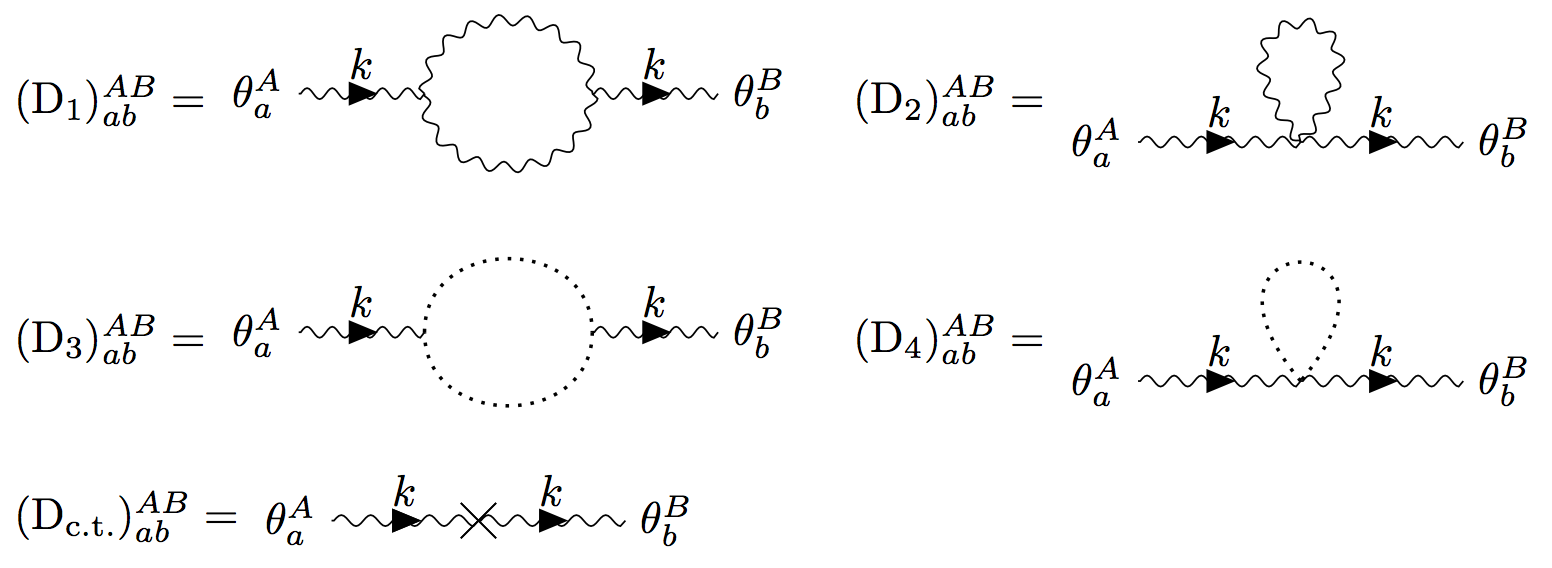
Figure 1: Self energy diagrams for $\theta_{a}$

IV.1.1 $\theta$ self energy diagram 1

Diagram 1 in Fig. 1 is given by

$$\left(\mathrm{D}_{1}\right)_{ab}^{AB} = \frac{1}{2}\int_{\ell}\sum_{cdef}\frac{\left(igV_{acd}^{ACD}\left(k,\ell\right)\right)\left(-i\delta^{CE}\delta_{ce}\right)\left(-i\delta^{DF}\delta_{ce}\right)\left(igV_{bef}^{BEF}\left(-k,-\ell\right)\right)}{\ell^{2}\ell_{c}^{2}\left(\ell+k\right)^{2}\left(\ell_{d}+k_{d}\right)^{2}}$$ (115)

$$= \frac{g^{2}}{2}f^{ACD}f^{BCD}\sum_{i=1}^{2}\sum_{j=1}^{2}\int\frac{d^{4}\ell}{\left(2\pi\right)^{4}}\sum_{cd}\frac{V_{acd}^{(i)}\left(k,\ell\right)V_{bcd}^{(j)}\left(-k,-\ell\right)}{\ell^{2}\left(\ell+k\right)^{2}\ell_{c}^{2}\left(\ell_{d}+k_{d}\right)^{2}}$$ (116)

$$= g^{2}C\left(A\right)\delta^{AB}\sum_{i=1}^{2}\sum_{j=1}^{2}\left(\mathrm{D}_{1}^{(i,j)}\right)_{ab}$$ (117)

where in the last line we define the sub-diagrams

$$\left(\mathrm{D}_{1}^{(i,j)}\right)_{ab}=\frac{1}{2}\int\frac{d^{4}\ell}{\left(2\pi\right)^{4}}\sum_{cd}\frac{V_{acd}^{(i)}\left(k,\ell\right)V_{bcd}^{(j)}\left(-k,-\ell\right)}{\ell^{2}\left(\ell+k\right)^{2}\ell_{c}^{2}\left(\ell_{d}+k_{d}\right)^{2}}$$ (118)

The sums over $i$ and $j$ in Eq. (117) only go from 1 to 2 because $\left(1-\frac{1}{\xi}\right)V_{abc}^{(3)}=0$ in the Feynman gauge. In the general $R_{\xi}$ gauge, the sums in Eq. (117) would go from 1 to 3. Due to the symmetry of the diagram, we also know that

$$\left(\mathrm{D}_{1}^{(j,i)}\right)_{ab}^{AB}\left(k\right)=\left(\mathrm{D}_{1}^{(i,j)}\right)_{ba}^{BA}\left(-k\right)$$ (119)

which means there are only three independent terms to compute in Eq. (117).

We start with

$$\left(\mathrm{D}_{1}^{(1,1)}\right)_{ab} =\frac{1}{2}\int\frac{d^{4}\ell}{\left(2\pi\right)^{4}}\sum_{cd}\frac{V_{acd}^{\left(1\right)}\left(k,\ell\right)V_{bcd}^{\left(1\right)}\left(-k,-\ell\right)}{\ell^{2}\left(\ell+k\right)^{2}\ell_{c}^{2}\left(\ell_{d}+k_{d}\right)^{2}}$$ (120)

$$=\frac{1}{2}\int\frac{d^{4}\ell}{\left(2\pi\right)^{4}}\sum_{cd}\frac{k_{a}k_{b}\ell_{c}^{2}\left(\ell_{d}+k_{d}\right)^{2}N_{abcd}}{\ell^{2}\left(\ell+k\right)^{2}\ell_{c}^{2}\left(\ell_{d}+k_{d}\right)^{2}}$$ (121)

$$=\frac{1}{2}k_{a}k_{b}\int\frac{d^{4}\ell}{\left(2\pi\right)^{4}}\frac{\sum_{cd}N_{abcd}}{\ell^{2}\left(\ell+k\right)^{2}}$$ (122)

where the numerator is

$$N_{abcd} = \left(-\delta_{cd}\left(2\ell_{a}+k_{a}\right)+\delta_{ad}\left(\ell_{c}+2k_{c}\right)+\delta_{ac}\left(\ell_{d}-k_{d}\right)\right)$$ (123)

$$\times\left(-\delta_{cd}\left(2\ell_{b}+k_{b}\right)+\delta_{bd}\left(\ell_{c}+2k_{c}\right)+\delta_{bc}\left(\ell_{d}-k_{d}\right)\right).$$

Summing over $c$ and $d$ yields

$$\sum_{cd}N_{abcd} = 10\ell_{a}\ell_{b}+5\ell_{a}k_{b}+5k_{a}\ell_{b}-2k_{a}k_{b}+\left(\left(\ell+2k\right)^{2}+\left(\ell-k\right)^{2}\right)\delta_{ab}$$ (124)

and applying this to Eq. (122) gives

$$\left(\mathrm{D}_{1}^{(1,1)}\right)_{ab} =\frac{1}{2}k_{a}k_{b}\int_{\ell}\frac{10\ell_{a}\ell_{b}+5\ell_{a}k_{b}+5k_{a}\ell_{b}-2k_{a}k_{b}+\left(\left(\ell+2k\right)^{2}+\left(\ell-k\right)^{2}\right)\delta_{ab}}{\ell^{2}\left(\ell+k\right)^{2}}$$ (125)

$$=\frac{1}{2}\tilde{k}_{a}^{\mu}\tilde{k}_{b}^{\nu}\int_{\ell}\frac{10\ell_{\mu}\ell_{\nu}+5\ell_{\mu}k_{\nu}+5k_{\mu}\ell_{\nu}-2k_{\mu}k_{\nu}+\left(\left(\ell+2k\right)^{2}+\left(\ell-k\right)^{2}\right)g_{\mu\nu}}{\ell^{2}\left(\ell+k\right)^{2}}.$$ (126)

The momentum integral of Eq. (126) is identical to the one that appears the usual non-Abelian $A_{\mu}$ formalism. We can evaluate it using the usual Feynman parameterization technique to obtain

$$\left(\mathrm{D}_{1}^{(1,1)}\right)_{ab}=\frac{1}{2}\tilde{k}_{a}^{\mu}\tilde{k}_{b}^{\nu}\int_{0}^{1}dx\int\frac{d^{d}q}{\left(2\pi\right)^{d}}\frac{\left(\frac{9}{2}q^{2}+\left(5-2x+2x^{2}\right)k^{2}\right)g_{\mu\nu}-\left(2+10x-10x^{2}\right)k_{\mu}k_{\nu}}{\left[q^{2}+x\left(1-x\right)k^{2}\right]^{2}}$$ (127)

We are only interested in the divergent part, which in dimensional regularization with $d=4-\epsilon$ is

$$\mathrm{div}\left(\left(\mathrm{D}_{1}^{(1,1)}\right)_{ab}\right)=\left(\frac{19}{12}k^{2}k_{a}^{2}\delta_{ab}-\frac{11}{6}k_{a}^{2}k_{b}^{2}\right)\frac{i}{8\pi^{2}\epsilon}$$ (128)

which has the same form numerically as the usual non-Abelian $A_{\mu}$ formalism.

We now compute

$$\left(\mathrm{D}_{1}^{(2,1)}\right)_{ab} =\frac{1}{2}\int\frac{d^{d}\ell}{\left(2\pi\right)^{d}}\sum_{cd}\frac{V_{acd}^{\left(2\right)}\left(k,\ell\right)V_{bcd}^{\left(1\right)}\left(-k,-\ell\right)}{\ell^{2}\left(\ell+k\right)^{2}\ell_{c}^{2}\left(\ell_{d}+k_{d}\right)^{2}}$$ (129)

$$=\frac{1}{4}\int\frac{d^{d}\ell}{\left(2\pi\right)^{d}}\frac{N_{ab}}{\ell^{2}\left(\ell+k\right)^{2}\ell_{a}^{2}\left(\ell_{a}+k_{a}\right)^{2}}$$ (130)

where the numerator is

$$N_{ab} = \left(\delta_{ab}-1\right)k_{b}\ell_{a}\left(\ell_{a}+k_{a}\right)\left(2\ell_{b}+k_{b}\right)$$ (131)

$$\times\left(k^{2}k_{a}\left(2\ell_{a}+k_{a}\right)-\ell^{2}\ell_{a}\left(\ell_{a}+2k_{a}\right)+\left(\ell+k\right)^{2}\left(\ell_{a}^{2}-k_{a}^{2}\right)\right).$$

The divergent part of Eq. (130) is

$$\mathrm{div}\left(\left(\mathrm{D}_{1}^{(2,1)}\right)_{ab}\right)=\frac{1}{4}\left(\delta_{ab}-1\right)k_{b}\left(4k^{2}k_{a}^{2}\delta_{ab}\frac{i}{8\pi^{2}\epsilon}\right)=0.$$ (132)

This is identically zero because of Eq. (113). Due to the symmetry of the diagram we also know that

$$\mathrm{div}\left(\left(\mathrm{D}_{1}^{(1,2)}\right)_{ab}\right)=0.$$ (133)

Finally, we compute

$$\left(\mathrm{D}_{1}^{(2,2)}\right)_{ab} = \frac{1}{2}\int\frac{d^{d}\ell}{\left(2\pi\right)^{d}}\sum_{cd}\frac{V_{acd}^{\left(2\right)}\left(k,\ell\right)V_{bcd}^{\left(2\right)}\left(k,\ell\right)}{\ell^{2}\left(\ell+k\right)^{2}\ell_{c}^{2}\left(\ell_{d}+k_{d}\right)^{2}}$$ (134)

$$= \frac{1}{8}\sum_{cd}\delta_{acd}\delta_{bcd}\int\frac{d^{d}\ell}{\left(2\pi\right)^{d}}\frac{n_{a}\left(k,\ell\right)n_{b}\left(k,\ell\right)}{\ell^{2}\left(\ell+k\right)^{2}\ell_{c}^{2}\left(\ell_{d}+k_{d}\right)^{2}}$$ (135)

$$= \frac{1}{8}\delta_{ab}\int\frac{d^{d}\ell}{\left(2\pi\right)^{d}}\frac{n_{a}\left(k,\ell\right)^{2}}{\ell^{2}\left(\ell+k\right)^{2}\ell_{a}^{2}\left(\ell_{a}+k_{a}\right)^{2}}$$ (136)

where

$$n_{a}\left(k,\ell\right)=k^{2}k_{a}\left(2\ell_{a}+k_{a}\right)-\ell^{2}\ell_{a}\left(\ell_{a}+2k_{a}\right)+\left(\ell+k\right)^{2}\left(\ell_{a}^{2}-k_{a}^{2}\right)\,.$$ (137)

The divergent part of Eq. (136) is

$$\mathrm{div}\left(\left(\mathrm{D}_{1}^{(2,2)}\right)_{ab}\right)=\frac{i}{8\pi^{2}\epsilon}\left(\frac{5}{2}k^{2}k_{a}^{2}\delta_{ab}\right).$$ (138)

After summing the contributions from the sub-diagrams given by Eqs. (128), (132), (133), and (138), we find that divergent part of the first diagram is

$$\mathrm{div}\left(\left(\mathrm{D}_{1}\right)_{ab}^{AB}\right)=C\left(A\right)\frac{g^{2}}{8\pi^{2}\epsilon}\left(\frac{49}{12}i\delta^{AB}k^{2}k_{a}^{2}\delta_{ab}-\frac{11}{6}i\delta^{AB}k_{a}^{2}k_{b}^{2}\right).$$ (139)

IV.1.2 $\theta$ self energy diagram 2

The second diagram is given by

$$\left(\mathrm{D}_{2}\right)_{ab}^{AB} =\frac{1}{2}\int\frac{d^{4}\ell}{\left(2\pi\right)^{4}}\sum_{cd}\left(\frac{-i\delta_{cd}\delta^{CD}}{\ell^{2}\ell_{c}^{2}}\right)iV_{abcd}^{ABCD}\left(k,-k,\ell,-\ell\right)$$ (140)

$$=\frac{g^{2}}{2}\int\frac{d^{4}\ell}{\left(2\pi\right)^{4}}\sum_{c}\sum_{i=1}^{6}\frac{V_{(i)abcc}^{ABCC}\left(k,-k,\ell,-\ell\right)}{\ell^{2}\ell_{c}^{2}};$$ (141)

the seventh and eighth terms of Eq. (141) don’t contribute because $\xi=1$. The following identity is useful in evaluating the divergent part of Eq. (141):

$$\mathrm{div}\left(\int\frac{d^{4}\ell}{\left(2\pi\right)^{4}}\frac{\ell_{a}^{N_{a}}\ell_{b}^{N_{b}}}{\ell^{2}\ell_{a}^{2}}\right) =\delta_{N_{a}0}\delta_{N_{b}0}\,\mathrm{div}\left(\int\frac{d^{4}\ell}{\left(2\pi\right)^{4}}\frac{1}{\ell^{2}\ell_{a}^{2}}\right)$$ (142)

$$=\delta_{N_{a}0}\delta_{N_{b}0}\frac{i\Gamma\left(\frac{\epsilon}{2}\right)\Gamma\left(-\frac{1}{2}\right)}{\left(4\pi\right)^{2}\Gamma\left(\frac{1}{2}\right)}$$ (143)

$$=\delta_{N_{a}0}\delta_{N_{b}0}\left(-\frac{i}{4\pi^{2}\epsilon}\right).$$ (144)

Since Eq. (144) is zero in dimensional regularization unless $N_{a}=N_{b}=0$, we ignore any term in the numerator of Eq. (141) that has any positive power of $\ell$ to find the divergence. We need to ignore any term that has $k_{3}=+\ell$ or $k_{4}=-\ell$ since they proportional to $\ell$.

The divergent part of the first four terms of Eq. (141) vanishes due to either Lorentz invariance or Eq. (144). The only non zero divergent contributions come from the fifth term, which is given by

$$V_{(5)abcc}^{ABCC} = 0+\frac{1}{4}f_{E}^{AC}f_{E}^{BC}\delta_{abc}\left[\left(k_{1}+k_{3}\right)^{2}\left(k_{1}-k_{3}\right)_{\star a}\left(k_{2}-k_{4}\right)\right.$$ (145)

$$\left.+\left(k_{1}+k_{4}\right)^{2}\left(k_{1}-k_{4}\right)_{\star a}\left(k_{2}-k_{3}\right)\right]$$

$$\rightarrow \frac{1}{4}f_{E}^{AC}f_{E}^{BC}\delta_{abc}\left(\left(k_{1}\right)^{2}k_{1\star a}k_{2}+\left(k_{1}\right)^{2}\left(k_{1}\right)_{\star a}\left(k_{2}\right)\right)$$ (146)

$$\rightarrow -\frac{1}{2}f_{E}^{AC}f_{E}^{BC}\delta_{ab}k^{2}k_{a}^{2},$$ (147)

and the sixth term, given by

$$V_{(6)abcc}^{ABCC} = \frac{1}{6}f_{E}^{AC}f_{E}^{BC}\delta_{abc}\left[k_{1}^{2}k_{1\star a}\left(k_{4}-k_{2}\right)+k_{3}^{2}k_{3\star a}\left(k_{2}-k_{4}\right)+k_{2}^{2}k_{2\star a}\left(k_{3}-k_{1}\right)+k_{4}^{2}k_{4\star a}\left(k_{1}-k_{3}\right)\right.$$ (148)

$$\left.+k_{1}^{2}k_{1\star a}\left(k_{3}-k_{2}\right)+k_{4}^{2}k_{4\star a}\left(k_{2}-k_{3}\right)+k_{2}^{2}k_{2\star a}\left(k_{4}-k_{1}\right)+k_{3}^{2}k_{3\star a}\left(k_{1}-k_{4}\right)\right]$$

$$\rightarrow \frac{1}{6}f_{E}^{AC}f_{E}^{BC}\delta_{ab}\left(k_{1}^{2}k_{1\star a}\left(-k_{2}\right)+k_{2}^{2}k_{2\star a}\left(-k_{1}\right)+k_{1}^{2}k_{1\star a}\left(-k_{2}\right)+k_{2}^{2}k_{2\star a}\left(-k_{1}\right)\right)$$

$$= +\frac{2}{3}f_{E}^{AC}f_{E}^{BC}\delta_{ab}k^{2}k_{a}^{2}.$$ (149)

Applying the results from Eq. (147) and Eq. (149) to Eq. (141) yields the following divergent contribution

$$\mathrm{div}\left(\left(\mathrm{D_{2}}\right)_{ab}^{AB}\right)=-\frac{1}{6}C\left(A\right)\frac{g^{2}}{8\pi^{2}\epsilon}\left(i\delta^{AB}k^{2}k_{a}^{2}\delta_{ab}\right).$$ (150)

IV.1.3 $\theta$ self energy diagram 3

The ghost-loop diagram 3 of Fig. 1 receives contributions from the ghosts of Eq. (57), which we label as $\mathrm{D_{3}^{(gh1)}}$ and the ghosts of Eq. (61), which we label as $\mathrm{D_{3}^{(gh2)}}$:

$$\left(\mathrm{D_{3}}\right)_{ab}^{AB}=\left(\mathrm{D_{3}^{(gh1)}}\right)_{ab}^{AB}+\left(\mathrm{\mathrm{D_{3}^{(gh2)}}}\right)_{ab}^{AB}$$ (151)

where

$$\left(\mathrm{D_{3}^{(gh1)}}\right)_{ab}^{AB} =\left(-1\right)\int_{p}igV_{a}^{A,CD}\left(k,p+k,p\right)\tfrac{1}{i}\Delta^{CF}\left(p+k\right)\tfrac{1}{i}\Delta^{DE}\left(p\right)igV_{b}^{B,EF}\left(-k,p,p+k\right)$$ (152)

$$=\left(-1\right)g^{2}\int\frac{d^{4}p}{\left(2\pi\right)^{4}}\frac{\left(f^{ACD}k_{\star a}\left(p+k\right)\right)\left(f^{BDC}\left(-k\right)_{\star b}p\right)}{p^{2}\left(p+k\right)^{2}}$$ (153)

$$=g^{2}f^{ACD}f^{BCD}\left(-\tilde{k}_{a}^{\mu}\tilde{k}_{b}^{\nu}\right)\int\frac{d^{4}p}{\left(2\pi\right)^{4}}\frac{\left(p+k\right)_{\mu}p_{\nu}}{p^{2}\left(p+k\right)^{2}}$$ (154)

and

$$\left(\mathrm{D_{3}^{(gh2)}}\right)_{ab}^{AB} =\left(-1\right)g^{2}\sum_{c,d}\int_{p}\frac{f^{ACD}\delta_{acd}\left(k-p\right)\star_{a}\left(p+k\right)f^{BDC}\delta_{bdc}\left(-k-p-k\right)\star_{a}p}{\left(p_{c}+k_{c}\right)^{2}p_{d}^{2}}$$ (155)

$$=-\frac{g^{2}}{4}C(A)\delta^{AB}\delta_{ab}\int_{p}\frac{\left(p_{a}-k_{a}\right)\left(p_{a}+k_{a}\right)\left(p_{a}+2k_{a}\right)p_{a}}{\left(p_{a}+k_{a}\right)^{2}p_{a}^{2}}.$$ (156)

Using the usual Feynman parameterization, the integral of Eq. (154) becomes

$$\int\frac{d^{d}p}{\left(2\pi\right)^{d}}\frac{\left(p+k\right)_{\mu}p_{\nu}}{p^{2}\left(p+k\right)^{2}} =\frac{i}{\left(4\pi\right)^{2}}\frac{2}{\epsilon}\int_{0}^{1}dx\left(-\frac{1}{2}g_{\mu\nu}x\left(1-x\right)k^{2}-x\left(1-x\right)k_{\mu}k_{\nu}\right)+\mathrm{finite}$$ (157)

$$=\frac{i}{8\pi^{2}\epsilon}\left(-\frac{1}{12}k^{2}g_{\mu\nu}-\frac{1}{6}k_{\mu}k_{\nu}\right)+\mathrm{finite}$$ (158)

and therefore

$$\mathrm{div}\left(\left(\mathrm{D_{3}^{(gh1)}}\right)_{ab}^{AB}\right)=i\delta^{AB}C\left(A\right)\frac{g^{2}}{8\pi^{2}\epsilon}\left(\frac{1}{12}k^{2}k_{a}^{2}\delta_{ab}+\frac{1}{6}k_{a}^{2}k_{b}^{2}\right).$$ (159)

The divergent part of $\mathrm{D_{3}^{(gh2)}}$ in dimensional regularization is zero because of Eq. (112) for $n=3$:

$$\mathrm{div}\left(\left(\mathrm{D_{3}^{(gh2)}}\right)_{ab}^{AB}\right)=0.$$ (160)

As noted before, it is interesting that the ghosts arising from transforming $A_{\mu}^{B}$ to $\theta_{c}^{A}$ do not contribute to the divergent structure here. Combining these results, we conclude that

$$\mathrm{div}\left(\left(\mathrm{D_{3}}\right)_{ab}^{AB}\right)=i\delta^{AB}C\left(A\right)\frac{g^{2}}{8\pi^{2}\epsilon}\left(\frac{1}{12}k^{2}k_{a}^{2}\delta_{ab}+\frac{1}{6}k_{a}^{2}k_{b}^{2}\right).$$ (161)

This ghost contribution will be important for restoring the transverse structure of the gauge boson propagator.

IV.1.4 $\theta$ self energy diagram 4

Similar to diagram 3, diagram 4 of Fig. 1 describes ghost contributions to the propagator. These however do not have any external momenta flowing through the ghost-lines. Just as in diagram 3, this has a contribution coming from the usual gauge-fixing ghost and the ghost associated with transforming the field coordinates from $A_{\mu}^{B}$ to $\theta_{c}^{A}$:

$$\left(\mathrm{D_{4}}\right)_{ab}^{AB}=\left(\mathrm{D_{4}^{(gh1)}}\right)_{ab}^{AB}+\left(\mathrm{D_{4}^{(gh2)}}\right)_{ab}^{AB}$$ (162)

We find the first ghost contribution to be

$$\left(\mathrm{D_{4}^{(gh1)}}\right)_{ab}^{AB} =\left(-1\right)\int\frac{d^{4}p}{\left(2\pi\right)^{4}}ig^{2}V_{ab}^{AB,CD}\left(k,-k,p,p\right)\tfrac{1}{i}\Delta^{CD}\left(p\right)$$ (163)

$$=\left(-1\right)\frac{g^{2}}{2}\int\frac{d^{4}p}{\left(2\pi\right)^{4}}\frac{f^{ABE}f^{CCE}\delta_{ab}2k_{a}p_{a}}{p^{2}}$$ (164)

$$=0$$ (165)

and the second ghost contribution to be

$$\left(\mathrm{D_{4}^{(gh2)}}\right)_{ab}^{AB} =\left(-1\right)\sum_{c}\int\frac{d^{4}p}{\left(2\pi\right)^{4}}ig^{2}V_{ab,cd}^{AB,CD}\left(k,-k,p,p\right)\tfrac{1}{i}\Delta_{cd}^{CD}\left(p\right)$$ (166)

$$=\frac{-ig^{2}}{6}\delta_{ab}\sum_{c}\int\frac{d^{4}p}{\left(2\pi\right)^{4}}\frac{f^{ACE}f^{BCE}\delta_{abc}\left(\left(p+k\right)\star_{a}p+\left(p-k\right)\star_{a}p\right)}{p_{a}^{2}}$$ (167)

$$=\frac{-ig^{2}}{6}f^{ACE}f^{BCE}\delta_{ab}\int\frac{d^{4}p}{\left(2\pi\right)^{4}}\frac{2p_{a}^{2}}{p_{a}^{2}}.$$ (168)

Using the identity Eq. (112), this also vanishes:

$$\mathrm{div}\left(\left(\mathrm{D_{4}^{(gh2)}}\right)_{ab}^{AB}\right)=0.$$ (169)

Therefore, we conclude

$$\mathrm{div}\left(\left(\mathrm{D}_{4}\right)_{ab}^{AB}\right)=0$$ (170)

and thus there are no external momentum independent ghost contribution to the divergent structure of the $\theta$ propagator in dimensional regularization.

IV.1.5 $\theta$ self energy counter-term

The counter-term diagram yields

$$\left(\mathrm{D_{c.t.}}\right)_{ab}^{AB} = -i\delta^{AB}\left((Z_{\theta^{2}}-1)\delta^{AB}\left(k^{2}k_{a}^{2}\delta_{ab}-k_{a}^{2}k_{b}^{2}\right)+\frac{1}{\xi}(Z_{\frac{1}{\xi}\theta^{2}}-1)k_{a}^{2}k_{b}^{2}\right)$$ (171)

$$= -i\delta^{AB}\left((Z_{\theta^{2}}-1)k^{2}k_{a}^{2}\delta_{ab}+(Z_{\frac{1}{\xi}\theta^{2}}-Z_{\theta^{2}})k_{a}^{2}k_{b}^{2}\right).$$ (172)

To have a finite self energy, we require the divergent parts of these diagrams to cancel out. The sum of Eqs. (139), (150), (161), and (170) is

$$\mathrm{div}\left(\sum_{i=1}^{4}\left(\mathrm{D}_{i}\right)_{ab}^{AB}\right)=i\delta^{AB}C\left(A\right)\frac{g^{2}}{8\pi^{2}\epsilon}\left(4k^{2}k_{a}^{2}\delta_{ab}-\frac{5}{3}k_{a}^{2}k_{b}^{2}\right)$$ (173)

and therefore the renormalization constants are

$$Z_{\theta^{2}} =1+4C\left(A\right)\frac{g^{2}}{8\pi^{2}\epsilon}$$ (174)

and

$$Z_{\frac{1}{\xi}\theta^{2}}=1+\frac{7}{3}C\left(A\right)\frac{g^{2}}{8\pi^{2}\epsilon}.$$ (175)

It is interesting that despite the nontransversality of the divergent part of the $\theta$ propagator seen here, the divergent part of the usual gauge field propagator when computed in the BTGT formalism will maintain transversality, as we will demonstrate below.

IV.1.6 Comment on $Z_{\frac{1}{\xi}\theta^{2}}$

Note that

$$Z_{\xi}=\frac{Z_{\theta^{2}}}{Z_{\frac{1}{\xi}\theta^{2}}}=1+\frac{5}{3}C\left(A\right)\frac{g^{2}}{8\pi^{2}\epsilon}=Z_{A^{2}}=\frac{Z_{A^{2}}}{Z_{\frac{1}{\xi}A^{2}}}$$ (176)

where $Z_{A^{2}}$ is gauge kinetic renormalization constant in the usual gauge theory formalism. This is a nontrivial check of the theory. It shows that $\xi_{B}=Z_{\xi}\xi_{R}$ has the same scaling behavior in BTGT as in the usual formalism. It is interesting that while $Z_{\frac{1}{\xi}A^{2}}=1$ to all orders in $g$, $Z_{\frac{1}{\xi}\theta^{2}}-1\neq 0$. This does not indicate a violation of gauge invariance because the gauge fixing parameter $\xi$ (parameterizing the coefficient of the gauge fixing chosen to be of the same form as in ordinary gauge theories with $A_{\mu}^{a}\rightarrow A_{\mu}^{a}[\theta]$) is still renormalized by the same renormalization constant of $Z_{\xi}$ as in the ordinary gauge theory formalism and $Z_{\theta^{2}}\neq Z_{A^{2}}$.

Another nontrivial check of the formalism would be to calculate $Z_{g\theta^{3}}$ and $Z_{\frac{1}{\xi}g\theta^{3}}$ and check that they satisfy

$$\frac{Z_{g\theta^{3}}}{Z_{\frac{1}{\xi}g\theta^{3}}}=1+\frac{5}{3}C\left(A\right)\frac{g^{2}}{8\pi^{2}\epsilon}+O\left(g^{4}\right)=Z_{\xi},$$ (177)

but we defer this to a future work.

IV.2 Computation of $Z_{\bar{c}c}$

The renormalization constant $Z_{\bar{c}c}$ is determined by the ghost self energy. The one loop diagrams that contribute to the ghost self energy are given in Fig. 2.

Figure 2: Ghost self energy diagrams

The first diagram in Fig. 2 is

$$\left(\mathrm{D_{1}}\right)^{AB}= g^{2}f^{CAD}f^{CDB}\sum_{c}\int_{\ell}\frac{\left(-\ell_{c}p_{c}\right)\ell_{c}\left(\ell_{c}+p_{c}\right)}{\ell_{c}^{2}\ell^{2}\left(\ell+p\right)^{2}}$$ (178)

$$= g^{2}C\left(A\right)\delta^{AB}\int_{\ell}\frac{p^{2}+p\cdot\ell}{\ell^{2}\left(\ell+p\right)^{2}}$$ (179)

$$= g^{2}C\left(A\right)\delta^{AB}p^{2}\int_{0}^{1}dx\left(1-x\right)\int_{q}\frac{1}{\left[q^{2}+x\left(1-x\right)p^{2}\right]^{2}}.$$ (180)

The divergent part of this is

$$\mathrm{div}\left(\left(\mathrm{D_{1}}\right)^{AB}\right) =-\frac{1}{2}C\left(A\right)\frac{g^{2}}{8\pi^{2}\epsilon}\left(-i\delta^{AB}p^{2}\right).$$ (181)

The second diagram in Fig. 2 vanishes identically because of the anti-symmetric property of $f^{CDE}$:

$$\left(\mathrm{D_{2}}\right)^{AB} =g^{2}\sum_{c,d}\int_{\ell}V_{cd}^{CD,AB}\left(\ell,-\ell,p\right)\Delta_{cd}^{CD}\left(\ell\right)$$ (182)

$$=g^{2}\sum_{c,d}\delta_{cd}\left(\frac{1}{2}f_{E}^{CD}f_{E}^{AB}\left(\ell_{c}+\ell_{c}\right)p_{c}\right)\frac{\delta_{cd}\delta^{CD}}{\ell^{2}\ell_{c}^{2}}$$ (183)

$$=0.$$ (184)

The counter-term diagram is given by

$$\left(\mathrm{D_{\mathrm{c.t.}}}\right)^{AB}=-i\left(Z_{\bar{c}c}-1\right)\delta^{AB}p^{2}.$$ (185)

In order to make the ghost self energy finite, we find that

$$Z_{\bar{c}c}=1+\frac{1}{2}C\left(A\right)\frac{g^{2}}{8\pi^{2}\epsilon}+O\left(g^{4}\right)\,.$$ (186)

Note that Eq. (186) is the same result that is obtained in the usual computation with $A_{\mu}^{a}$ fields. This is most likely part of a general result discussed in more detail in IV.4.

IV.3 Computation of $Z_{g\theta\bar{c}c}$

Let’s now compute the $\theta_{a}$-ghost interaction in our continuing efforts to derive Eq. (105). The relevant diagrams are defined in Fig. 3.

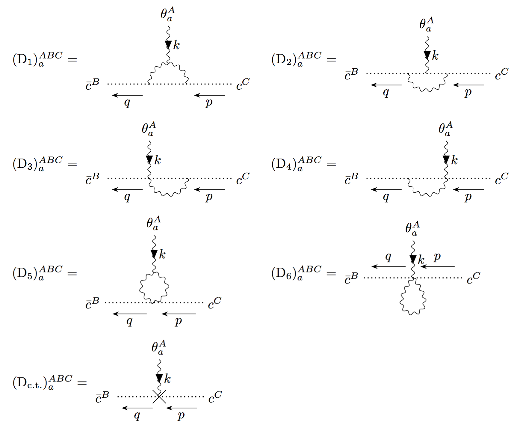
Figure 3: Ghost-$\theta$ vertex one loop diagrams

One of the surprises in the computation below will be that the first diagram $D_{1}$ of Fig. 3 vanishes. This is in contrast with the case in which $\theta_{a}^{A}$ is replaced by $A_{\mu}^{A}$. Another interesting aspect of the computation will be that diagrams $D_{3}$ and $D_{4}$ each violate the BTGT symmetry in the divergence, but their sum has a cancellation that thereby preserves the BTGT symmetry.

IV.3.1 Ghost-$\theta$ vertex diagrams 1 and 2

Diagram 1 in Fig. 3 is given by

$$\left(\mathrm{D_{1}}\right)_{a}^{ABC} =g^{3}f^{EBD}f^{FDC}f^{AEF}\sum_{e,f}\int_{\ell}\frac{\left(-\ell_{e}q_{e}\right)\left(\ell_{f}+k_{f}\right)\left(\ell_{f}+q_{f}\right)\left(V_{aef}^{(1)}\left(k,\ell\right)+V_{aef}^{(2)}\left(k,\ell\right)\right)}{\ell^{2}\left(\ell+k\right)^{2}\left(\ell+q\right)^{2}\ell_{e}^{2}\left(\ell_{f}+k_{f}\right)^{2}}$$ (187)

$$=\left(\mathrm{D_{1}^{\left(1\right)}}\right)_{a}^{ABC}+\left(\mathrm{D_{1}^{\left(2\right)}}\right)_{a}^{ABC}$$ (188)

where we have denoted the $V_{aef}^{(n)}$ contributions as $D_{1}^{(n)}$ which we will evaluate separately. Through the identity

$$f^{AEF}f^{EBD}f^{FDC}=-f_{A}^{FE}f_{B}^{ED}f_{C}^{DF}=-\frac{1}{2}f^{ABC}C\left(A\right),$$ (189)

the first contribution can be written as

$$\left(\mathrm{D_{1}^{\left(1\right)}}\right)_{a}^{ABC}= -\frac{g^{3}}{2}f^{ABC}C\left(A\right)\sum_{e,f}\int_{\ell}\frac{\left(-\ell_{e}q_{e}\right)\left(\ell_{f}+k_{f}\right)\left(\ell_{f}+q_{f}\right)V_{aef}^{\left(1\right)}(k,\ell)}{\ell^{2}\left(\ell+k\right)^{2}\left(\ell+q\right)^{2}\ell_{e}^{2}\left(\ell_{f}+k_{f}\right)^{2}}$$ (190)

$$= -\frac{g^{3}}{2}f^{ABC}C\left(A\right)k_{a}$$

$$\times\int_{\ell}\frac{q_{a}\left(\ell+q\right)\cdot\left(k-\ell\right)-\left(\ell_{a}+q_{a}\right)q\cdot\left(\ell+2k\right)+\left(2\ell_{a}+k_{a}\right)q\cdot\left(\ell+q\right)}{\ell^{2}\left(\ell+k\right)^{2}\left(\ell+q\right)^{2}}\,.$$ (191)

A divergence only occurs when the numerator is at $\ell^{2}$ or higher powers in $\ell$. There are no terms higher than $\ell^{2}$ and therefore the maximum degree of divergence is zero. This means that we can ignore the dependence on the external momenta in the denominator:

$$\mathrm{div}\left(\left(\mathrm{D_{1}^{\left(1\right)}}\right)_{a}^{ABC}\right) =-\frac{g^{3}}{2}f^{ABC}C\left(A\right)k_{a}\mathrm{div}\left(\int_{\ell}\frac{\left(\ell\cdot q\right)\ell_{a}-\ell^{2}q_{a}}{\ell^{2}\left(\ell+k\right)^{2}\left(\ell+q\right)^{2}}\right)$$ (192)

$$=-\frac{g^{3}}{2}f^{ABC}C\left(A\right)k_{a}\left(-\frac{3}{4}q_{a}\frac{i}{8\pi^{2}\epsilon}\right)$$ (193)

$$=+\frac{3}{8}C\left(A\right)\frac{g^{2}}{8\pi^{2}\epsilon}\left(igf^{ABC}k_{a}q_{a}\right)\,.$$ (194)

The second contribution to this diagram is

$$\left(\mathrm{D_{1}^{\left(2\right)}}\right)_{a}^{ABC} = -\frac{g^{3}}{2}f^{ABC}C\left(A\right)\sum_{e,f}\int_{\ell}\frac{\left(-\ell_{e}q_{e}\right)\left(\ell_{f}+k_{f}\right)\left(\ell_{f}+q_{f}\right)V_{aef}^{\left(2\right)}(k,\ell)}{\ell^{2}\left(\ell+k\right)^{2}\left(\ell+q\right)^{2}\ell_{e}^{2}\left(\ell_{f}+k_{f}\right)^{2}}$$ (196)

$$= \frac{1}{4}g^{3}f^{ABC}C\left(A\right)q_{a}\int_{\ell}\ell_{a}\left(\ell_{a}+k_{a}\right)\left(\ell_{a}+q_{a}\right)$$

$$\times\frac{\left(k^{2}k_{a}\left(2\ell_{a}+k_{a}\right)-\ell^{2}\ell_{a}\left(\ell_{a}+2k_{a}\right)+\left(\ell+k\right)^{2}\left(\ell_{a}^{2}-k_{a}^{2}\right)\right)}{\ell^{2}\left(\ell+k\right)^{2}\left(\ell+q\right)^{2}\ell_{a}^{2}\left(\ell_{a}+k_{a}\right)^{2}}\,.$$

The divergent part evaluates to

$$\mathrm{div}\left(\left(\mathrm{D_{1}^{\left(2\right)}}\right)_{a}^{ABC}\right) =-\frac{3}{8}C\left(A\right)\frac{g^{2}}{8\pi^{2}\epsilon}\left(igf^{ABC}k_{a}q_{a}\right)\,.$$ (197)

Summing these contributions together gives

$$\mathrm{div}\left(\left(\mathrm{D_{1}}\right)_{a}^{ABC}\right)=\left(+\frac{3}{8}-\frac{3}{8}\right)C\left(A\right)\frac{g^{2}}{8\pi^{2}\epsilon}\left(igf^{ABC}k_{a}q_{a}\right)=0\,.$$ (198)

The result of the diagram $D_{1}$ calculation with $\theta_{a}^{A}$ replaced with $A_{\mu}^{A}$ is equivalent to Eq. (194) (see e.g. Grozin:2005yg ). The difference between this result and Eq. (198) is a manifestation of how $\theta_{a}^{A}$ is different from $A_{\mu}^{A}$.

Diagram 2 is given by

$$\left(\mathrm{D_{2}}\right)_{a}^{ABC} =g^{3}\sum_{f}\int_{\ell}\frac{V_{f}^{F,BD}\left(-\ell+p,q\right)V_{a}^{A,DE}\left(k,\ell+k\right)V_{f}^{F,EC}\left(\ell-p,\ell\right)}{\left(\ell+k\right)^{2}\ell^{2}\left(\ell-p\right)^{2}\left(\ell_{f}-p_{f}\right)^{2}}$$ (199)

$$=g^{3}f^{FBD}f^{ADE}f^{FEC}\sum_{f}\int_{\ell}\frac{\left(-\ell_{f}+p_{f}\right)q_{f}k_{a}\left(\ell_{a}+k_{a}\right)\left(\ell_{f}-p_{f}\right)\ell_{f}}{\left(\ell+k\right)^{2}\ell^{2}\left(\ell-p\right)^{2}\left(\ell_{f}-p_{f}\right)^{2}}$$ (200)

$$=\frac{g^{3}}{2}C\left(A\right)f^{ABC}k_{a}\int_{\ell}\frac{\left(\ell_{a}+k_{a}\right)\sum_{f}q_{f}\ell_{f}}{\left(\ell+k\right)^{2}\ell^{2}\left(\ell-p\right)^{2}},$$ (201)

and the divergent part of this diagram is therefore

$$\mathrm{div}\left(\left(\mathrm{D_{2}}\right)_{a}^{ABC}\right)=+\frac{1}{8}C\left(A\right)\frac{g^{2}}{8\pi^{2}\epsilon}\left(if^{ABC}k_{a}q_{a}\right).$$ (202)

The $1/8$ coefficient here is obtained when we replaces the $\theta_{a}^{A}$ with $A_{\mu}^{A}$ in the usual gauge theory.

IV.3.2 Ghost-$\theta$ vertex diagram 3 and 4

Diagram 3 evaluates to

$$\left(\mathrm{D_{3}}\right)_{a}^{ABC} =g^{3}\int_{\ell}\sum_{d}\frac{V_{ad}^{AD,BE}\left(k,-\ell;q,\ell+p\right)V_{d}^{D,EC}\left(\ell;\ell+p,p\right)}{\ell^{2}\ell_{d}^{2}\left(\ell+p\right)^{2}}$$ (203)

$$=\frac{1}{2}g^{3}f_{F}^{AD}f_{F}^{BE}f^{DEC}\sum_{d}\int_{\ell}\frac{\delta_{ad}\left(k_{d}+\ell_{d}\right)q_{d}\ell_{d}\left(\ell_{d}+p_{d}\right)}{\ell^{2}\ell_{d}^{2}\left(\ell+p\right)^{2}}$$ (204)

$$=\frac{1}{4}g^{3}C\left(A\right)f^{ABC}q_{a}\int_{\ell}\frac{\left(\ell_{a}+k_{a}\right)\ell_{a}\left(\ell_{a}+p_{a}\right)}{\ell^{2}\left(\ell+p\right)^{2}\ell_{a}^{2}}$$ (205)

and after integrating, we find the divergent part is

$$\mathrm{div}\left(\left(\mathrm{D_{3}}\right)_{a}^{ABC}\right) =\frac{1}{4}C\left(A\right)\frac{g^{2}}{8\pi^{2}\epsilon}\left(igf^{ABC}\right)\left(\frac{1}{2}q_{a}k_{a}+\frac{1}{2}q_{a}^{2}\right).$$ (206)

Diagram 4 evaluates to

$$\left(\mathrm{D_{4}}\right)_{a}^{ABC} =g^{3}\int_{\ell}\sum_{d}\frac{V_{d}^{D,BE}\left(-\ell;q,\ell+p\right)V_{ad}^{AD,EC}\left(k,\ell;\ell+q,p\right)}{\ell^{2}\ell_{d}\left(\ell+q\right)^{2}}$$ (207)

$$=\frac{1}{2}g^{3}f^{DBE}f_{F}^{AD}f_{F}^{EC}\int_{\ell}\sum_{d}\frac{\left(-\ell_{d}q_{d}\right)\delta_{ad}\left(k_{a}-\ell_{a}\right)\left(\ell_{a}+q_{a}\right)}{\ell^{2}\left(\ell+q\right)^{2}\ell_{d}^{2}}$$ (208)

$$=-\frac{1}{4}g^{3}C\left(A\right)f^{ABC}q_{a}\int_{\ell}\frac{\ell_{a}\left(\ell_{a}-k_{a}\right)\left(\ell_{a}+q_{a}\right)}{\ell^{2}\left(\ell+q\right)^{2}\ell_{a}^{2}},$$ (209)

and the divergent part is

$$\mathrm{div}\left(\left(\mathrm{D_{4}}\right)_{a}^{ABC}\right) =\frac{1}{4}C\left(A\right)\frac{g^{2}}{8\pi^{2}\epsilon}\left(igf^{ABC}\right)\left(q_{a}k_{a}-\frac{1}{2}q_{a}^{2}\right)\,.$$ (210)

Even though the divergent parts of $\mathrm{D_{3}}$ and $\mathrm{D_{4}}$ separately lead to new counter terms that would violate BTGT and gauge invariance, their sum does not. The BTGT violating term proportional to $q_{a}^{2}$ cancels and we are left with

$$\mathrm{div}\left(\left(\mathrm{D_{3}}\right)_{a}^{ABC}+\left(\mathrm{D_{4}}\right)_{a}^{ABC}\right)=\frac{3}{8}C\left(A\right)\frac{g^{2}}{8\pi^{2}\epsilon}\left(igf^{ABC}q_{a}k_{a}\right)\,.$$ (211)

This contribution does not have an analog in the ordinary gauge theory formalism in which there is no quartic coupling of the gauge sector to the ghosts.

IV.3.3 Ghost-$\theta$ vertex diagram 5

Diagram 5 in Fig. 3 is given by

$$\mathrm{\left(D_{5}\right)}_{a}^{ABC} =\frac{g^{3}}{2}\sum_{d,e}\int_{\ell}\frac{V_{ade}^{ADE}\left(k,\ell\right)V_{de}^{DE,BC}\left(-\ell,\ell+k;q,p\right)}{\ell^{2}\left(\ell+k\right)^{2}\ell_{d}^{2}\left(\ell_{e}+\ell_{e}\right)^{2}}$$ (212)

$$=\frac{g^{3}}{2}\sum_{d,e}\int_{\ell}\frac{f^{ADE}V_{ade}\left(k,\ell\right)\frac{1}{2}\delta_{de}f_{F}^{DE}f_{F}^{BC}q_{d}\left(-2\ell_{d}-k_{d}\right)}{\ell^{2}\left(\ell+k\right)^{2}\ell_{d}^{2}\left(\ell_{e}+\ell_{e}\right)^{2}}$$ (213)

$$=-\frac{g^{3}}{4}C\left(A\right)f^{ABC}\sum_{d}\int_{\ell}\frac{V_{add}\left(k,\ell\right)q_{d}\left(2\ell_{d}+k_{d}\right)}{\ell^{2}\left(\ell+k\right)^{2}\ell_{d}^{2}\left(\ell_{d}+k_{d}\right)^{2}}$$ (214)

$$=\left(\mathrm{D_{5}^{(1)}}\right)_{a}^{ABC}+\left(\mathrm{D_{5}^{(2)}}\right)_{a}^{ABC}\,.$$ (215)

We find that

$$\mbox{div}\left(\left(\mathrm{D_{5}^{\left(1\right)}}\right)_{a}^{ABC}\right)=0,$$ (216)

$$\mbox{div}\left(\mathrm{D_{5}^{\left(2\right)}}\right)=-\frac{3}{2}C\left(A\right)\frac{g^{2}}{8\pi^{2}\epsilon}\left(igf^{ABC}q_{a}k_{a}\right),$$ (217)

and $\mathrm{D_{5}^{\left(3\right)}}=0$ in the Feynman gauge. The total divergent component of this diagram is thus

$$\mathrm{div}\left(\mathrm{\left(D_{5}\right)}_{a}^{ABC}\right)=-\frac{3}{2}C\left(A\right)\frac{g^{2}}{8\pi^{2}\epsilon}\left(igf^{ABC}q_{a}k_{a}\right)\,.$$ (218)

Diagram 6 in Fig. 3 is

$$\left(\mathrm{D_{6}}\right)_{a}^{ABC} =\frac{1}{2}g^{3}\sum_{d}\int_{\ell}\frac{V_{add}^{ADD,BC}\left(k,\ell,-\ell;p,q\right)}{\ell^{2}\ell_{d}^{2}}$$ (219)

$$=\frac{1}{12}g^{3}\sum_{d}\int_{\ell}\frac{\delta_{add}q_{a}f_{F}^{BC}\left(0+f_{G}^{FD}f_{G}^{DA}\left(k_{a}+\ell_{a}\right)+f_{G}^{FD}f_{G}^{AD}\left(\ell_{a}-k_{a}\right)\right)}{\ell^{2}\ell_{d}^{2}}$$ (220)

$$=\frac{1}{12}g^{3}f_{F}^{BC}\left(-C\left(A\right)\delta^{AF}\right)q_{a}\int_{\ell}\frac{2k_{a}}{\ell^{2}\ell_{a}^{2}}\,.$$ (221)

The divergent part turns out to be

$$\mathrm{div}\left(\left(\mathrm{D_{6}}\right)_{a}^{ABC}\right)=+\frac{1}{3}C\left(A\right)\frac{g^{2}}{8\pi^{2}\epsilon}\left(igf^{ABC}q_{a}k_{a}\right)\,.$$ (222)

IV.3.4 Counter term and the conclusion of the explicit computation of the beta function

The counter term is

$$\left(\mathrm{D_{c.t.}}\right)_{a}^{ABC}=\left(Z_{g\theta\bar{c}c}-1\right)\left(igf^{ABC}q_{a}k_{a}\right)\,.$$ (223)

After summing the contributions from Eqs. (198), (202), (211), (218), and (222), we immediately find the renormalization constant

$$Z_{g\theta\bar{c}c}=1+\frac{2}{3}C\left(A\right)\frac{g^{2}}{8\pi^{2}\epsilon}+O\left(g^{4}\right).$$ (224)

Hence, we have finally accomplished our computation of the $Z_{g}$ given by Eq. (110) using the non-Abelian BTGT formalism. Thus, as mentioned at the beginning of this section where we embarked on an explicit computation of the beta function, it is gratifying to see that the $\theta_{a}^{A}$ formalism can be used to reproduce the perturbative results of the $A_{\mu}^{A}$ formalism. The true physics advantage of using the non-Abelian BTGT formalism has yet to be discovered, but its existence is expected since simple correlators in $\theta_{a}^{A}$ will map to nonlinear and nonlocal $A_{\mu}^{B}$ correlators.

IV.4 Callan-Symanzik Equation and the beta function

Here we give another perspective on the beta function computation which we have explicitly carried out in the previous subsections. We expect the correlator $\left\langle\Psi\overline{\Psi}\right\rangle$ to be independent of the gauge formalism chosen for any matter or ghost field $\Psi$ because the change from the $A_{\mu}$ formalism to $\theta_{a}$ formalism does not depend on $\Psi$. In other words, assuming

$$\left\langle\Psi\overline{\Psi}\right\rangle^{(A)}=\left\langle\Psi\overline{\Psi}\right\rangle^{(\theta)},$$ (225)

and using the Callan–Symanzik equation

$$\left[\frac{\partial}{\partial\ln\mu}+\beta\left(g\right)\frac{\partial}{\partial g}-\xi\frac{\partial\ln Z_{\xi}}{\partial\ln\mu}\frac{\partial}{\partial\xi}+\frac{\partial\ln Z_{\Psi\Psi}}{\partial\ln\mu}\right]\left\langle\Psi\overline{\Psi}\right\rangle=0,$$ (226)

we infer that

$$\beta^{\left(A\right)}\left(g\right)=\beta^{\left(\theta\right)}\left(g\right),$$ (227)

$$Z_{\xi}^{(A)}=Z_{\xi}^{(\theta)},$$ (228)

and

$$Z_{\Psi\Psi}^{\left(A\right)}=Z_{\Psi\Psi}^{\left(\theta\right)}.$$ (229)

Even more generally, the anomalous dimension of any matter or ghost field should be independent of the gauge formalism.

V Composite operator correlator

One of the key differences of non-Abelian BTGT from Abelian BTGT is the appearance of the nonlinearity in the map between the $\theta_{a}^{A}$ variable and the ordinary gauge field $A_{\mu}^{A}$ variable. Hence, any $A_{\mu}^{A}[\theta]$ correlator computation in ordinary field theory turns into a composite operator correlation computation beyond the leading order in the coupling constant expansion. To demonstrate explicitly that we can recover the gauge dynamics of $A_{\mu}^{A}$ at the quantum level using the non-Abelian BTGT formalism, we give in this section an example of the requisite composite operator renormalization. We will find that the transverse divergent structure of the two-point function is recovered only after including the composite operator renormalization, indicating the self-consistency of the formalism and that ordinary gauge invariance is not spoiled by the nonlinear field redefinition and the BTGT symmetry. We will also show in this section that there is a sufficient number of counter term coefficients to preserve finiteness of both $\theta_{a}^{A}$ and $A_{\mu}^{B}$ correlators without spoiling the gauge and BTGT symmetries, lending further evidence that the $\theta_{a}^{A}$ theory is a consistent rewriting of the $A_{\mu}^{A}$ theory.

More explicitly, define the two-point momentum space Green’s function by

$$G_{\mu\nu}^{AB}\left(k\right) =\int d^{4}x\,e^{-ik\cdot x}\left\langle A_{\mu}^{A}\left(x\right)A_{\nu}^{B}\left(0\right)\right\rangle$$ (230)

$$=\int d^{4}x\,e^{-ik\cdot x}\left.\frac{\delta}{i\delta J^{\mu A}\left(x\right)}\frac{\delta}{i\delta J^{\nu B}\left(0\right)}\bar{Z}\left[J,K\right]\right|_{J=0,K=0}$$ (231)

where $\bar{Z}\left[J,K\right]$ is the generating function defined in Eq. (100). The difference from the usual generating function Eq. (99) is that $A_{\mu}$ is now a composite operator in terms of $\theta_{a}$ fields and the path integral is now over $\theta_{a}$ instead of $A_{\mu}$. Using dimensional regularization with $d=4-\epsilon$, we will demonstrate below that the divergent part of the momentum space Green’s function for $A_{\mu}$ is transverse and exactly the same as the typical formulation before introducing counter terms.

$$\mathrm{div}\left(G_{\mu\nu}^{AB}\left(k\right)\right) = \frac{5}{3}C\left(A\right)\frac{g^{2}}{8\pi^{2}\epsilon}\frac{1}{i}\delta^{AB}\left(\frac{g_{\mu\nu}}{k^{2}}-\frac{k_{\mu}k_{\nu}}{k^{4}}\right)$$ (232)

$$+\mathrm{div}\left(\left(\mathrm{D}_{c.t.1}\right)_{\mu\nu}^{AB}+\left(\mathrm{D}_{c.t.2}\right)_{\mu\nu}^{AB}+\left(\mathrm{D_{c.t.3}}\right)_{\mu\nu}^{AB}\right)$$

Furthermore, after introducing counter terms, we will find that both $\left\langle\theta_{a}^{A}\theta_{b}^{B}\right\rangle$ and $\left\langle A_{\mu}^{A}A_{\nu}^{B}\right\rangle$ can be made finite without changing the symmetries of the theory. The details of the $\left\langle A_{\mu}^{A}A_{\nu}^{B}\right\rangle$ computation are presented below.

This calculation simplifies significantly when using the Feynman gauge. This is due to the gauge propagator becoming diagonal in the BTGT indices, which greatly simplifies the sums.

V.1 Tree level

The tree level diagram for the two-point $A_{\mu}$ correlator in the Feynman gauge is

$$= \sum_{a,b}\left(-i\tilde{k}_{\mu}^{a}\right)\tfrac{1}{i}\Delta_{ab}^{AB}\left(k\right)\left(i\tilde{k}_{\nu}^{b}\right)$$ (234)

$$= -i\frac{\delta^{AB}}{k^{2}}\sum_{a}\frac{\tilde{k}_{\mu}^{a}\tilde{k}_{\nu}^{a}}{k_{a}^{2}}$$ (235)

$$= -i\frac{\delta^{AB}}{k^{2}}\sum_{a}(H^{a})_{\mu\nu}$$ (236)

$$= -i\frac{\delta^{AB}}{k^{2}}g_{\mu\nu}$$ (237)

as expected. The structure is essentially identical to Abelian BTGT at this level of approximation.

V.2 Source operator terms

Next we consider the one-loop diagrams determining the composite operator counter-terms. The diagrams involved in evaluating $\left\langle A_{\mu}^{A}A_{\nu}^{B}\right\rangle$ at one loop are shown in Fig. 4.

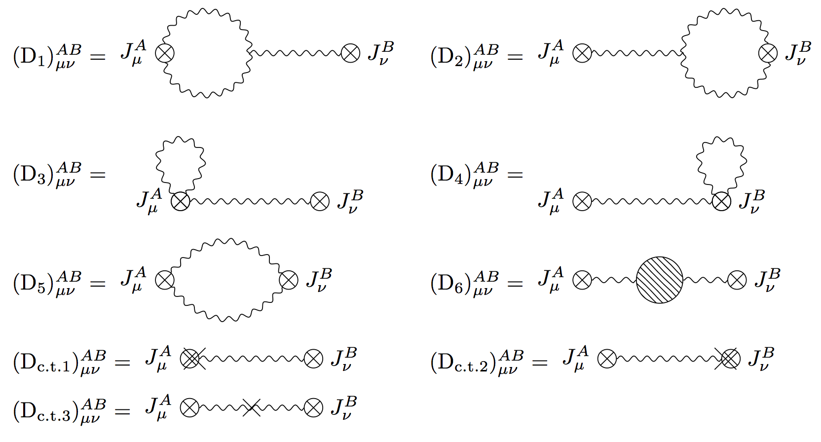
Figure 4: Diagram to compute the $A_{\mu}\left[\theta\right]$ two-point correlator. The blob in $\mathrm{D}_{6}$ refers to all 1PI sub-diagrams and is proportional to the $\theta_{a}$ self energy. A further breakdown is shown in Fig. 5.

The first diagram in Fig. 4 is given by

$$\left(\mathrm{D}_{1}\right)_{\mu\nu}^{AB}=\sum_{i=1}^{2}\left(\mathrm{D_{1}^{(i)}}\right)_{\mu\nu}^{AB}$$ (238)

where $i$ runs through the two possible terms of the $\theta^{3}$ vertex and

$$\left(\mathrm{D}_{1}^{(i)}\right)_{\mu\nu}^{AB}=\frac{g^{2}}{4}C\left(A\right)\delta^{AB}\sum_{a,b}\int\frac{d^{d}\ell}{\left(2\pi\right)^{d}}\frac{\left(2\tilde{\ell}_{\mu}^{a}+\tilde{k}_{\mu}^{a}\right)V_{baa}^{\left(i\right)}\left(k,\ell\right)}{\ell_{a}^{2}\ell^{2}\left(\ell_{a}+k_{a}\right)^{2}\left(\ell+k\right)^{2}}\frac{\tilde{k}_{\nu}^{b}}{k_{b}^{2}k^{2}}.$$ (239)

The $\theta^{3}$ vertex in Eq. (239) can be written as

$$V_{baa}^{\left(1\right)}\left(k,\ell\right) = k_{b}\ell_{a}\left(\ell_{a}+k_{a}\right)\left(\delta_{ab}-1\right)\left(2\ell_{b}+k_{b}\right)$$ (240)

$$V_{baa}^{\left(2\right)}\left(k,\ell\right) = \frac{1}{2}\delta_{ab}\left(k^{2}k_{a}\left(2\ell_{a}+k_{a}\right)-\ell^{2}\ell_{a}\left(\ell_{a}+2k_{a}\right)+\left(\ell+k\right)^{2}\left(\ell_{a}^{2}-k_{a}^{2}\right)\right)$$ (241)

where there is no sum over $a$ or $b$. Using Eq. (240), we find

$$\left(\mbox{D}_{1}^{\left(1\right)}\right)_{\mu\nu}^{AB} =\frac{g^{2}}{4}C\left(A\right)\delta^{AB}\sum_{a,b}\frac{k_{b}\tilde{k}_{\nu}^{b}}{k_{b}^{2}k^{2}}\left(\delta_{ab}-1\right)\int\frac{d^{d}\ell}{\left(2\pi\right)^{d}}\frac{\left(2\tilde{\ell}_{\mu}^{a}+\tilde{k}_{\mu}^{a}\right)\ell_{a}\left(\ell_{b}+k_{b}\right)\left(\ell_{a}-k_{a}\right)}{\ell_{a}^{2}\ell^{2}\left(\ell_{a}+k_{a}\right)^{2}\left(\ell+k\right)^{2}}$$ (242)

$$=\frac{g^{2}}{4}C\left(A\right)\delta^{AB}\sum_{a,b}\frac{k_{b}\tilde{k}_{b}^{\nu}}{k_{b}^{2}k^{2}}\left(\delta_{ab}-1\right)\left(2\delta_{\mu}^{a}\delta_{ab}\frac{i}{8\pi^{2}\epsilon}+\mathrm{finite}\right)$$ (243)

$$=0+\mathrm{finite}.$$ (244)

From Eq. (241), we find

$$\left(\mathrm{D_{1}^{(2)}}\right)_{\mu\nu}^{AB} = \frac{g^{2}}{8}C\left(A\right)\delta^{AB}\sum_{a}\frac{\tilde{k}_{a}^{\nu}}{k_{a}^{2}k^{2}}\left(\left(12\tilde{k}_{a}^{\mu}\right)\frac{i}{8\pi^{2}\epsilon}+\mbox{finite}\right)$$ (245)

$$= -\frac{3}{2}C\left(A\right)\frac{g^{2}}{8\pi^{2}\epsilon}\left(\frac{1}{i}\delta^{AB}\frac{g^{\mu\nu}}{k^{2}}\right)+\mbox{finite.}$$ (246)

Adding up the contributions gives

$$\mathrm{div}\left(\left(\mathrm{D_{1}}\right)_{\mu\nu}^{AB}\right)=-\frac{3}{2}C\left(A\right)\frac{g^{2}}{8\pi^{2}\epsilon}\left(\frac{1}{i}\delta^{AB}\frac{g^{\mu\nu}}{k^{2}}\right).$$ (247)

The symmetry between diagrams 1 and 2 of Fig. 4 is given $\left\{A,k\right\}\leftrightarrow\left\{B,-k\right\}$, and we can therefore conclude without computation

$$\mathrm{div}\left(\left(\mathrm{D_{2}}\right)_{\mu\nu}^{AB}\right)=-\frac{3}{2}C\left(A\right)\frac{g^{2}}{8\pi^{2}\epsilon}\left(\frac{1}{i}\delta^{AB}\frac{g^{\mu\nu}}{k^{2}}\right).$$ (248)

The third diagram in Fig. 4 is given by

$$\left(\mbox{D}_{3}\right)_{\mu\nu}^{AB} = \frac{1}{2}\sum_{b,b^{\prime},c,d}\int_{\ell}ig^{2}V_{\mu,b^{\prime}cd}^{A,B^{\prime}CD}\left(k;-k,\ell,-\ell\right)\tfrac{1}{i}\Delta_{b^{\prime}b}^{B^{\prime}B}\left(k\right)\tfrac{1}{i}\Delta_{cd}^{CD}\left(\ell\right)i\tilde{k}_{\nu}^{b}$$ (249)

$$= \frac{g^{2}}{12}\sum_{b,c}\frac{\tilde{k}_{\nu}^{b}}{k^{2}k_{b}^{2}}\int_{\ell}\delta_{bcc}\frac{0+f_{E}^{AC}f_{E}^{BC}\left(-\tilde{\ell}_{\mu}^{b}+\tilde{k}_{\mu}^{b}\right)+f_{E}^{AC}f_{E}^{BC}\left(\tilde{\ell}_{\mu}^{b}+\tilde{k}_{\mu}^{b}\right)}{\ell^{2}\ell_{c}^{2}}$$ (250)

$$= +\frac{1}{3}C\left(A\right)\frac{g^{2}}{8\pi^{2}\epsilon}\left(\frac{1}{i}\delta^{AB}\frac{g_{\mu\nu}}{k^{2}}\right)+\mathrm{finite}.$$ (251)

Since the fourth diagram in Fig. 4 must be the same as $\mathrm{D}_{3}$ up to $\left\{A,k\right\}\leftrightarrow\left\{B,-k\right\}$, we can immediately write

$$\mathrm{div}\left(\left(\mathrm{D}_{4}\right)_{\mu\nu}^{AB}\right)=+\frac{1}{3}C\left(A\right)\frac{g^{2}}{8\pi^{2}\epsilon}\left(\frac{1}{i}\delta^{AB}\frac{g_{\mu\nu}}{k^{2}}\right).$$ (252)

Diagram 5 in Fig. 4 is

$$\left(\mathrm{D}_{5}\right)_{\mu\nu}^{AB}=\frac{1}{2}\sum_{a,b}\left(\frac{g}{2}\right)^{2}\int\frac{d^{d}\ell}{\left(2\pi\right)^{d}}\frac{f^{ACD}\left(-2\tilde{\ell}_{\mu}^{a}-\tilde{k}_{\mu}^{a}\right)f^{BCD}\left(2\tilde{\ell}_{\nu}^{b}+\tilde{k}_{\nu}^{b}\right)}{\ell^{2}\ell_{a}^{2}\left(\ell+k\right)^{2}\left(\ell_{b}+k_{b}\right)^{2}}.$$ (253)

This momentum integral does not UV diverge for $d=4$: i. e.

$$\mathrm{div}\left(\left(\mathrm{D}_{5}\right)_{\mu\nu}^{AB}\right)=0.$$ (254)

V.3 $\theta$ self energy diagrams

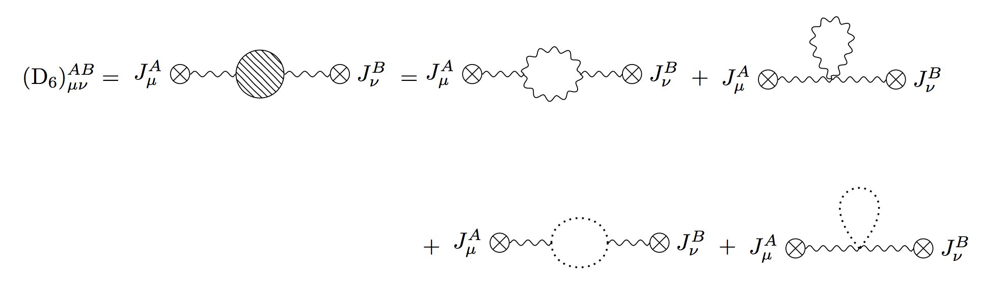
Figure 5: Breakdown of $\left(\mathrm{D_{6}}\right)_{\mu\nu}^{AB}$ from Fig. 4; they are equivalent to the $\theta_{a}$ self energy diagrams of Fig. 1.

Diagram 6 in Fig. 4 is the sum of all 1PI sub-diagrams as shown in Fig. 5. Using the results of Section IV.1, we have

$$\mathrm{div}\left(\Pi_{ab}^{AB}\left(k\right)\right)=C\left(A\right)\frac{g^{2}}{8\pi^{2}\epsilon}\delta^{AB}\left(4k^{2}k_{a}^{2}\delta_{ab}-\frac{5}{3}k_{a}^{2}k_{b}^{2}\right)$$ (255)

where $\Pi_{ab}^{AB}\left(k\right)$ is the $\theta_{a}$ self energy. The divergent part of diagram 6 is given by

$$\mathrm{div}\left(\left(\mathrm{D_{6}}\right)_{\mu\nu}^{AB}\right) =\sum_{a,b,a^{\prime},b^{\prime}}\left(-i\tilde{k}_{\mu}^{a}\right)\tfrac{1}{i}\Delta_{aa^{\prime}}^{AA^{\prime}}\left(k\right)\mathrm{div}\left(i\Pi_{a^{\prime}b^{\prime}}^{A^{\prime}B^{\prime}}\left(k\right)\right)\tfrac{1}{i}\Delta_{b^{\prime}b}^{B^{\prime}B}\left(k\right)\left(i\tilde{k}_{\nu}^{b}\right)$$ (256)

$$=-\sum_{a,b}\frac{\tilde{k}_{\mu}^{a}\tilde{k}_{\nu}^{b}}{k^{4}k_{a}^{2}k_{b}^{2}}i\mathrm{div}\left(\Pi_{ab}^{AB}\left(k\right)\right)$$ (257)

$$=C\left(A\right)\frac{g^{2}}{8\pi^{2}\epsilon}\frac{1}{i}\delta^{AB}\left(4\frac{g_{\mu\nu}}{k^{2}}-\frac{5}{3}\frac{k_{\mu}k_{\nu}}{k^{4}}\right).$$ (258)

As expected, the divergences of Fig. 5 are completely canceled out by the renormalization constants $Z_{\theta^{2}}$ and $Z_{\frac{1}{\xi}\theta^{2}}$ that arise from $\mathrm{D_{c.t.3}}$ in Fig. 4.

V.4 Renormalization

Adding up the contributions from the six diagrams of Fig. 4, given by Eqs. (247), (248), (251), (252), (254), and (258) gives the divergent part of the two-point $A$ correlator before renormalization:

$$\sum_{i=1}^{6}\mathrm{div}\left(\left(\mathrm{D_{i}}\right)_{\mu\nu}^{AB}\right) =C\left(A\right)\frac{g^{2}}{8\pi^{2}\epsilon}\frac{1}{i}\delta^{AB}\left(\left(-3+\frac{2}{3}+4\right)\frac{g_{\mu\nu}}{k^{2}}-\frac{5}{3}\frac{k_{\mu}k_{\nu}}{k^{4}}\right)$$ (259)

$$=\frac{5}{3}C\left(A\right)\frac{g^{2}}{8\pi^{2}\epsilon}\frac{1}{i}\delta^{AB}\left(\frac{g_{\mu\nu}}{k^{2}}-\frac{k_{\mu}k_{\nu}}{k^{4}}\right).$$ (260)

It has the expected transverse property and the same numerical value as in the usual $A_{\mu}$ formulation. While the $k_{\mu}k_{\nu}$ term receives a contribution from only diagram $\mathrm{D_{6}}$, the $g_{\mu\nu}$ term receives contributions from six diagrams $\mathrm{D}_{1}$ through $\mathrm{D}_{6}$.

Now we need to renormalize both $\theta_{a}$ and the composite operator $A_{\mu}[\theta]$ and show that both correlators are finite without introducing any counter terms that spoil gauge invariance, BTGT invariance, or Lorentz invariance. The composite operator counter terms in the Lagrangian are of the form

$$\mathcal{L}_{c.t.}\ni\left(Z_{J\theta}-1\right)J^{A\mu}\tilde{\partial}_{\mu}^{a}\theta_{a}^{A}+\left(Z_{gJ\theta^{2}}-1\right)\frac{g}{2}f^{ABC}J^{A\mu}\tilde{\partial}_{\mu}^{a}\theta_{a}^{B}\theta^{C}+\dots$$ (261)

and to preserve BTGT invariance the counter terms have to obey certain relations given by

$$Z_{J}=\frac{Z_{J\theta}}{Z_{\theta^{2}}^{1/2}}=\frac{Z_{Jg\theta^{2}}}{Z_{g}Z_{\theta^{2}}}=\frac{Z_{Jg^{2}\theta^{3}}}{Z_{g}^{2}Z_{\theta^{2}}^{3/2}}=\dots$$ (262)

where we have defined $Z_{J}$ to be the ratio of the bare source $J_{0}$ to the renormalized source $J$: $J_{0}\equiv Z_{J}J$ .

The $Z_{J\theta}$ counter-term occurs in diagrams $\mathrm{D}_{c.t.1}$ and $\mathrm{D}_{c.t.2}$ of Fig. 4, which evaluate to

$$\left(\mathrm{D}_{c.t.1}\right)_{\mu\nu}^{AB} =\sum_{a,b}\left(-i\left(Z_{J\theta}-1\right)\tilde{k}_{\mu}^{a}\right)\tfrac{1}{i}\Delta_{ab}^{AB}\left(k\right)\left(i\tilde{k}_{\nu}^{b}\right)$$ (263)

$$=\left(Z_{J\theta}-1\right)\frac{1}{i}\frac{\delta^{AB}}{k^{2}}\sum_{a}\frac{\tilde{k}_{\mu}^{a}\tilde{k}_{\nu}^{a}}{k_{a}^{2}}$$ (264)

$$=\left(Z_{J\theta}-1\right)\left(-i\frac{\delta^{AB}}{k^{2}}g_{\mu\nu}\right)\,,$$ (265)

and

$$\left(\mathrm{D}_{c.t.2}\right)_{\mu\nu}^{AB} =\sum_{a,b}\left(-i\tilde{k}_{\mu}^{a}\right)\tfrac{1}{i}\Delta_{ab}^{AB}\left(k\right)\left(i\left(Z_{J\theta}-1\right)\tilde{k}_{\nu}^{b}\right)$$ (266)

$$=\left(Z_{J\theta}-1\right)\left(-i\frac{\delta^{AB}}{k^{2}}g_{\mu\nu}\right)\,.$$ (267)

Using the results of Section IV.1, we find

$$\left(\mathrm{D_{c.t.3}}\right)_{\mu\nu}^{AB} = \sum_{a,b,a^{\prime},b^{\prime}}-i\tilde{k}_{\mu}^{a}\tfrac{1}{i}\Delta_{aa^{\prime}}^{AA^{\prime}}\left(k\right)\tfrac{1}{i}\delta^{AB}\left(\left(Z_{\theta^{2}}-1\right)k^{2}k_{a}^{2}\delta_{ab}+\left(Z_{\frac{1}{\xi}\theta^{2}}-Z_{\theta^{2}}\right)k_{a}^{2}k_{b}^{2}\right)$$

$$\times\tfrac{1}{i}\Delta_{b^{\prime}b}^{B^{\prime}B}\left(k\right)i\tilde{k}_{\nu}^{b}$$

$$= \sum_{a,b}\frac{\tilde{k}_{\mu}^{a}\tilde{k}_{\nu}^{b}}{k^{4}k_{a}^{2}k_{b}^{2}}i\delta^{AB}\left(4C\left(A\right)\frac{g^{2}}{8\pi^{2}\epsilon}k^{2}k_{a}^{2}\delta_{ab}-\frac{5}{3}C\left(A\right)\frac{g^{2}}{8\pi^{2}\epsilon}k_{a}^{2}k_{b}^{2}\right)+O\left(g^{4}\right)$$ (269)

$$= C\left(A\right)\frac{g^{2}}{8\pi^{2}\epsilon}\frac{\delta^{AB}}{i}\left(-4\frac{g_{\mu\nu}}{k^{2}}+\frac{5}{3}\frac{k_{\mu}k_{\nu}}{k^{4}}\right)+O\left(g^{4}\right)\,.$$ (270)

The divergence of all these diagrams cancel to make the two-point $A_{\mu}$ correlator finite:

$$\mathrm{div}\left(G_{\mu\nu}^{AB}\left(k\right)\right) =\mathrm{div}\left(\sum_{i=1}^{6}\left(\mathrm{D}_{i}\right)_{\mu\nu}^{AB}+\left(\mathrm{D}_{c.t.1}\right)_{\mu\nu}^{AB}+\left(\mathrm{D}_{c.t.2}\right)_{\mu\nu}^{AB}+\left(\mathrm{D_{c.t.3}}\right)_{\mu\nu}^{AB}\right)$$ (271)

$$=\left(\frac{7}{3}C\left(A\right)\frac{g^{2}}{8\pi^{2}\epsilon}+2\mbox{div}\left(Z_{J\theta}\right)\right)\left(-i\frac{\delta^{AB}}{k^{2}}g_{\mu\nu}\right)$$ (272)

$$=0\,.$$ (273)

The renormalization constant $Z_{J\theta}$ is therefore

$$Z_{J\theta}=1+\frac{7}{6}C\left(A\right)\frac{g^{2}}{8\pi^{2}\epsilon}+O\left(g^{4}\right)\,.$$ (274)

Using this, Eq. (107), and Eq. (262), we see that

$$Z_{J}^{-1}=\frac{Z_{\theta^{2}}^{1/2}}{Z_{J\theta}}=1+\frac{5}{6}C\left(A\right)\frac{g^{2}}{8\pi^{2}\epsilon}+O\left(g^{4}\right)=Z_{A^{2}}^{1/2}\,.$$ (275)

The self-consistency of the renormalization, $Z_{\theta^{2}}^{1/2}/Z_{J\theta}$ equals $Z_{A^{2}}^{1/2}$, is as expected from the external source coupling in the usual $A_{\mu}^{A}$ theory being of the form

$$\mathcal{L}_{J}\ni J^{\mu A}A_{\mu}^{A}$$ (276)

where $A_{\mu}^{A}$ are renormalized fields, while in the BTGT formulation the source coupling is defined with a composite operator renormalization constant $Z_{J\theta}$ as seen in Eq. (261).

VI Counter term predictions and Slavnov-Taylor identities

The Slavnov-Taylor identities have yet to be formally derived or shown to exist for the BTGT formalism. This is an interesting area for future study. The one loop calculations done thus far show that $g$ and $\xi$ scale as expected, and $A$ scales as expected when written as a composite operator of $\theta$. Assuming that the symmetries in BTGT are preserved in a way similar to the explicitly computed processes in this paper, we state in this section a set of concrete generalizations for the one loop counter term factors for the $\theta^{n}$-vertex.

We expect the BTGT formulation of the Slavnov-Taylor identities to show that the following holds

$$Z_{g^{n-2}\theta^{n}} =Z_{g}^{n-2}Z_{\theta^{2}}^{n/2}\qquad\left(n\geq 2\right)$$ (277)

$$Z_{\xi^{-1}g^{n-2}\theta^{n}} =Z_{\xi}^{-1}Z_{g}^{n-2}Z_{\theta^{2}}^{n/2}\qquad\left(n\geq 2\right)$$ (278)

$$Z_{g^{n}\theta^{n}\bar{c}c} =Z_{\bar{c}c}Z_{g}^{n}Z_{\theta^{2}}^{n/2}\qquad\left(n\geq 0\right).$$ (279)

Based on calculated value in Eq. (174), the predictions are

$$Z_{g^{n-2}\theta^{n}} =1+\frac{22+n}{6}C\left(A\right)\frac{g^{2}}{8\pi^{2}\epsilon}+O\left(g^{4}\right)\qquad\left(n\geq 2\right)$$ (280)

$$Z_{\xi^{-1}g^{n-2}\theta^{n}} =1+\frac{12+n}{6}C\left(A\right)\frac{g^{2}}{8\pi^{2}\epsilon}+O\left(g^{4}\right)\qquad\left(n\geq 2\right)$$ (281)

$$Z_{g^{n}\theta^{n}\bar{c}c} =1+\frac{3+n}{6}C\left(A\right)\frac{g^{2}}{8\pi^{2}\epsilon}+O\left(g^{4}\right)\qquad\left(n\geq 0\right).$$ (282)

We have explicitly computed the $n=2$ case of Eq. (280) and Eq. (281) and also the $n=0$ and $n=1$ cases of Eq. (282). An interesting and nontrivial check of BTGT in the future is the $n=3$ case of Eq. (280) and Eq. (281), which is given by the triple gauge $\theta^{3}$ vertex diagrams. Also of interest is the $n=2$ case of Eq. (282), which corresponds to the $\theta^{2}\bar{c}c$ vertex.

The factors $Z_{g}$, $Z_{\xi}$ and $Z_{\bar{c}c}$ are unchanged by the choice of using either the BTGT field $\theta_{a}$ or the vector potential $A_{\mu}$ to describe the gauge boson sector. We could have started by assuming that the following relations would hold:

$$Z_{g}^{(\theta)}=Z_{g}^{(A)} =1-\frac{11}{6}C\left(A\right)\frac{g^{2}}{8\pi^{2}\epsilon}+O\left(g^{4}\right)$$ (283)

$$Z_{\xi}^{(\theta)}=Z_{\xi}^{(A)} =1+\frac{5}{3}C\left(A\right)\frac{g^{2}}{8\pi^{2}\epsilon}+O\left(g^{4}\right)$$ (284)

$$Z_{\bar{c}c}^{(\theta)}=Z_{\bar{c}c}^{(A)} =1+\frac{1}{2}C\left(A\right)\frac{g^{2}}{8\pi^{2}\epsilon}+O\left(g^{4}\right),$$ (285)

where $Z^{(\theta)}$ is calculated in $\theta_{a}$ formalism and $Z^{(A)}$ in the $A_{\mu}$ formalism. Therefore, $Z_{\theta^{2}}$ is the only a priori undetermined parameter in Eqs. (277), (278), and (282) . Since we have done four computations and there was only one a priori undetermined parameter, we have done three independent nontrivial checks of the gauge invariance of this theory at one loop level. This result gives us confidence that gauge invariance in the BTGT formalism is preserved in perturbation theory.

VII Conclusions

We have constructed a non-Abelian basis tensor gauge theory (BTGT) which gives an alternate formulation of usual non-Abelian gauge theory in terms of the vierbein analog for ordinary gauge bundles. For example, the basis tensor that couples to matter transforming as $N$ of $SU(N)$ has the representation $\bar{N}$ and has the Lorentz transformation properties of a rank 2 projection tensor. To match the usual gauge theory formalism, the basis tensor must satisfy Eq. (17) and the couplings must be symmetric under a non-gauge symmetry called BTGT symmetry that is identical to the BTGT transformation of the Abelian case. To have a simple match in the number of degrees of freedom between the ordinary gauge theory formalism and the BTGT formalism, we have decided to choose the scalar fields $\theta_{a}^{A}$ that parameterize the basis tensor to be in the target space of the gauge manifold just as in Abelian BTGT. As in the Abelian BTGT case, the map between $\theta_{c}^{F}$ is a nonlocal functional of $A_{\mu}^{B}$. More explicitly, $\theta_{c}$ is a type of path-ordered line integral of $A_{\mu}$, and hence is related to Wilson lines. However, unlike in the Abelian case, the map between $A_{\mu}^{B}$ and $\theta_{c}^{F}$ is nonlinear, where the nonlinearities form a power series of the structure constants. This means that any $A_{\mu}^{B}$ correlator computation is a composite operator correlator with respect to the $\theta_{c}^{F}$ elementary field theory requiring composite operator counter terms.

The Feynman rules for the 1-loop order and $O(g^{2})$ computations were explicitly presented. We have tested non-Abelian BTGT to one-loop and $O(g^{2})$ (where $g$ is the usual gauge coupling), using $\theta_{c}^{F}$ are the elementary field degrees of freedom, by computing the beta function of the gauge coupling and finding it to be identical to the usual formulation. We have also computed the gauge field 2-point function to the same one-loop accuracy and found identical results as in the usual gauge theory formulation. In particular, we found that the UV divergent part of the correlator is transverse just as in the usual gauge theory formulation. Furthermore, the composite operator counter terms are sufficient to make both the $A_{\mu}^{B}$ correlator and $\theta_{c}^{F}$ correlators finite.

Through these explicit computations, we have also given several nontrivial checks that the renormalization constants in the minimal subtraction scheme are identical to those of the usual gauge theory formalism. Although we defer a formal BRST construction for this theory to a future work, the nontrivial checks indicate that there will be no insurmountable obstacles to its formulation.

Although the nonlinearities in the map between $A_{\mu}^{B}$ and $\theta_{a}^{C}$ might make this choice of formalism seem unnecessarily complicated, it is a natural choice from several considerations. First, it leads to a natural match in the number of functional degrees of freedom of a gauge theory. Second, it is a continuous deformation (as a function of group structure constants) of a simple linear map in the case of Abelian theories. Third, its semblance with nonlinear sigma-model parameterizations may allow several extensions of this work using the techniques that have been developed for sigma models. Fourth, the BTGT symmetry which stabilizes the Hamiltonian and the gauge symmetry have elegant representations given by Eqs. (10) and (26). Note also that from the perspective of having a nontrivial transformation that may lead to new insights into the usual gauge theory formulations, such nonlinear maps are more promising. On the other hand, it is important to keep in mind, just as in the usual sigma model parameterizations, this choice of using $\theta_{a}^{C}$ is far from unique even though there is uniqueness of the map between the vierbein-like field $\left[G_{(f)}(x)\right]_{\phantom{\gamma}\delta}^{\gamma}$ (which $\theta_{a}^{C}$ parameterizes) and the gauge field $A_{\mu}$ if we stipulate that the gauged matter kinetic term be locally gauge equivalent to that without a gauge field.

Many extensions of this work on BTGT theory beyond explicit constructions of BRST formalism are self-evident. To complete the tests of this formalism’s equivalence with the usual Standard Model formulation, BTGT should also be tested in the contexts of spontaneous symmetry breaking and curved spacetime. Since this is a formalism most naturally suited for exploring Wilson lines, it would be interesting to reformulate the Eikonal phase re-summing soft gluonic effects Alday:2008yw ; Korchemsky:1992xv ; Korchemsky:1991zp ; Frenkel:1984pz ; Catani:1983bz in this formalism and investigate whether any new insights or simplifications can arise. The enhanced local nature of BTGT for dealing with nonlocal quantities such as Wilson lines also suggests exploring its applications in lattice gauge theory Kronfeld:2012uk ; Brambilla:2014jmp . The gauge field representation $iU_{a}\tilde{\partial}_{\mu}^{a}U_{a}^{\dagger}$ also is reminiscent of the sigma model representation used in Witten:1983tw to explore topological aspects of the theories with spontaneously broken global symmetries. This suggests there may be a way to more conveniently explore the topological aspects of gauge theories using the BTGT formalism. The precise connection between the generalized global symmetries of Gaiotto:2014kfa and the symmetries of BTGT remains to be clarified. For physics beyond the standard model, it would be interesting to see if the gauge fields can be interpreted as Nambu-Goldstone bosons of a spontaneously broken theory since $A_{\mu}=iU_{a}\tilde{\partial}_{\mu}^{a}U_{a}^{\dagger}$ are suggestive of a sigma model.

Appendix A Relevant Notation

This section lists the various notations and conventions used throughout this paper. The metric signature chosen was

$$g_{\mu\nu}=\mathrm{diag}(-,+,+,+)\,\,.$$ (286)

If $\psi_{(a)}^{\mu}$ for $a\in\{0,1,2,3\}$ are 4 orthonormal Lorentz 4-vectors, we can write an explicit representation of the projection tensors $(H^{a})_{\phantom{\mu}\nu}^{\mu}$ as

$$(H^{a})_{\phantom{\mu}\nu}^{\mu}=\psi_{(a)}^{\mu}\psi_{(a)\nu}g^{aa}\,.$$ (287)

The $H^{a}$ matrices are commutative.

Using these projection tensors $(H^{a})_{\phantom{\mu}\nu}^{\mu}$, we define the following notation related to them. We define the tilde notation as

$$\tilde{A}_{a}^{\mu}\equiv(H^{a})_{\phantom{\mu}\nu}^{\mu}A^{\nu}$$ (288)

to denote the contraction between $H^{a}$ and any 4-vector $A^{\mu}$. Note that $\tilde{A}^{a\mu}=\tilde{A}_{a}^{\mu}$ because there is no covariant/contravariant distinction for the BTGT index unlike a Lorentz index $\mu$. Also, we define the star product as

$$A\star_{a}B\equiv\left(H^{a}\right)_{\mu\nu}A^{\mu}B^{\nu}$$ (289)

for any two 4-vectors $A^{\mu}$ and $B^{\mu}$. Using the tilde notation defined above, we have the following identities

$$A\star_{a}B=\tilde{A}_{a}^{\mu}B_{\mu}=A_{\mu}\tilde{B}_{a}^{\mu}=g_{\mu\nu}\tilde{A}_{a}^{\mu}\tilde{B}_{a}^{\nu}$$ (290)

We define the product of two Kronecker deltas as

$$\delta_{abc}\equiv\delta_{ab}\delta_{bc}=\delta_{ac}\delta_{bc}=\delta_{ab}\delta_{ac}\qquad\mbox{no sum over $a,b,c$}\,.$$ (291)

moving to Euclideanized space via Wick rotation , we can unambiguously define for any four vector $p^{\mu}$

$$p_{a}\equiv\psi_{(a)}^{\mu}p_{\mu}$$ (292)

that satisfies

$$p\star_{a}p=p_{a}^{2}\quad\mbox{and}\quad\sum_{a=0}^{3}p_{a}^{2}=p^{2}\,.$$ (293)

The group structure constant $f^{ABC}$ is defined by the Lie bracket

$$\left[T^{A},T^{B}\right]=if^{ABC}T^{C}$$ (294)

where $T^{A}$ are basis elements of the Lie algebra such that $e^{iT^{A}\Gamma^{A}}$ are group elements for some function $\Gamma^{A}\left(x\right)$. We take the basis of generators such that $f^{ABC}$ is completely anti-symmetric. Given this anti-symmetry, we can define without ambiguity the following

$$f_{C}^{AB}=f_{AB}^{C}=f^{ABC}\,\,.$$ (295)

Note that $f_{C}^{AB}=f_{B}^{CA}=f_{A}^{BC}$.

Note that Ref. Chung:2016lhv uses the notation of having the basis tensor index $c$ of $\theta^{c}$ (with $c\in\{1,2,3,4\}$) instead of $\theta_{c}^{B}$ (with $c\in\{0,1,2,3\}$) as in Eq. (5). Also, the sign convention for $\theta$ has been flipped between Eq. (23) of Ref. Chung:2016lhv and Eq. (5).

In the Feynman diagrams, all momenta that flow into a vertex are assigned a positive value.

Appendix B The relationship between non-Abelian basis tensor and ordinary gauge fields $A_{\mu}$

Here we follow the equivalence-principle-like procedure of Chung:2016lhv to construct the relationship of non-Abelian basis tensor and the ordinary non-Abelian gauge field $A_{\mu}(x)$.

Start with a gauge frame such that the Lagrangian at spacetime point $x_{1}$ looks like there is no gauge field (i.e. trivial Chern-Simons number vacuum):

$$\mathcal{L}_{\phi}(x_{1})=\partial_{\mu}\tilde{\phi}^{a}\partial^{\mu}\tilde{\phi}^{*a}(x_{1}).$$ (296)

We demand in this special gauge frame that the vierbein-like tensor field has the following value at point $x_{1}$:

$$\tilde{G}_{\alpha\beta}(x_{1})=S_{\alpha\beta}(x_{1}).$$ (297)

Upon making a gauge transformation to move to the general frame, we have

$$\phi(x)=e^{i\theta^{C}(x)T^{C}}\tilde{\phi}(x),$$ (298)

The gauge field in the new frame is

$$\tilde{D}_{\mu}\tilde{\phi}=\tilde{g}^{-1}D_{\mu}\tilde{g}\tilde{g}^{-1}\phi$$ (299)

where

$$\tilde{g}=e^{i\theta^{C}(x)T^{C}}.$$ (300)

Hence, we find

$$\partial_{\mu}\tilde{\phi}=\tilde{g}^{-1}(\partial_{\mu}-iA_{\mu})\phi$$ (301)

where the right hand side can be also be written in terms of $\tilde{\phi}$ as

$$\partial_{\mu}\tilde{\phi}=\left[\partial_{\mu}+\tilde{g}^{-1}\partial_{\mu}\tilde{g}-i\tilde{g}^{-1}A_{\mu}\tilde{g}\right]\tilde{\phi}.$$ (302)

This implies

$$0=\left[\tilde{g}^{-1}\partial_{\mu}\tilde{g}-i\tilde{g}^{-1}A_{\mu}\tilde{g}\right]\tilde{\phi}$$ (303)

or equivalently

$$A_{\mu}(x_{1})=-i\left[\partial_{\mu}\tilde{g}(x_{1})\right]\tilde{g}^{-1}(x_{1})$$ (304)

which is pure gauge only at a single point $x_{1}$ and not for all spacetime (just as in the Abelian construction).

We can use Eq. (304) to find the map between $G_{\alpha\beta}$ and $A_{\mu}$. Since $G_{\alpha\beta}$ is defined to obey the transformation rule of Eq. (3):

$$G_{(f)\,\beta}^{\alpha}(x_{1})\phi(x_{1})=\tilde{G}_{(f)\,\beta}^{\alpha}(x_{1})\tilde{\phi}(x_{1})$$ (305)

where

$$\phi(x_{1})=\tilde{g}(x_{1})\tilde{\phi}(x_{1}).$$ (306)

This means

$$G_{(f)\,\beta}^{\alpha}(x_{1})=\tilde{G}_{(f)\,\beta}^{\alpha}(x_{1})\tilde{g}^{-1}(x_{1}).$$ (307)

Similarly as in Chung:2016lhv , choose $\partial_{\alpha}\tilde{G}_{(f)\,\beta}^{\alpha}(x_{1})=0$. To solve for the right hand side of Eq. (304), we take the derivative

$$\left[G_{(f)\beta\mu}\right]^{m}\left[\partial_{\alpha}\tilde{g}\right]^{ml}+\left[\partial_{\alpha}G_{(f)\beta\mu}\right]^{m}\left[\tilde{g}\right]^{ml}=0$$ (308)

Let

$$\delta^{ks}=\sum_{f}^{{\rm dim}R}\xi_{(f)}^{k}\xi_{(f)}^{*s}$$ (309)

where the $\xi_{(f)}$ are constant vectors in the group representation space. This allows us to rewrite Eq. (308) as

$$\xi_{(f)}^{*s}\left[G_{\beta\mu}\right]^{sm}\left[\partial_{\alpha}\tilde{g}\right]^{ml}+\xi_{(f)}^{*s}\left[\partial_{\alpha}G_{\beta\mu}\right]^{sm}\left[\tilde{g}\right]^{ml}=0$$ (310)

where

$$\xi_{(f)}^{*s}\left[G_{\beta\mu}\right]^{sm}\equiv\left[G_{(f)\beta\mu}\right]^{m}.$$ (311)

Multiplying both sides by $\xi_{(f)}^{q}$ and summing, we find

$$\sum_{f}\xi_{(f)}^{q}\xi_{(f)}^{*s}\left[G_{\beta\mu}\right]^{sm}\left[\partial_{\alpha}\tilde{g}\right]^{ml}=-\sum_{f}\xi_{(f)}^{q}\xi_{(f)}^{*s}\left[\partial_{\alpha}G_{\beta\mu}\right]^{sm}\left[\tilde{g}\right]^{ml}$$ (312)

to arrive at

$$\left[G_{\beta\mu}\right]^{qm}\left[\partial_{\alpha}\tilde{g}\right]^{ml}=-\left[\partial_{\alpha}G_{\beta\mu}\right]^{qm}\left[\tilde{g}\right]^{ml}$$ (313)

Require that the inverse of $\left[G_{\beta\mu}\right]^{qm}$ exists such that

$$\left[G^{-1\lambda\beta}\right]^{bq}\left[G_{\beta\mu}\right]^{qm}=\delta_{\,\,\,\,\,\,\mu}^{\lambda}\delta^{bm}$$ (314)

Eq. (313) then becomes

$$\delta_{\,\,\,\,\,\,\mu}^{\lambda}\left[\partial_{\alpha}\tilde{g}\right]^{bl}\left[\tilde{g}^{-1}\right]^{ls}=-\left[G^{-1\lambda\beta}\right]^{bq}\left[\partial_{\alpha}G_{\beta\mu}\right]^{qs}$$ (315)

After setting $\lambda=\alpha$, we sum over $\alpha$ to obtain

$$A_{\mu}=i\left[G^{-1\alpha\beta}\right]\left[\partial_{\alpha}G_{\beta\mu}\right]$$ (316)

where Eq. (311) gives the explicit relationship to the basis tensor as

$$\left[G_{\beta\mu}\right]^{qm}=\sum_{f}^{{\rm dim}R}\xi_{(f)}^{q}\left[G_{(f)\beta\mu}\right]^{m}.$$ (317)

Eq. (316) can also be expressed in terms of derivative of the basis tensor $G_{(f)\beta\mu}$ as

$$A_{\mu}=i\sum_{f}^{{\rm dim}R}\left[G^{-1\alpha\beta}\right]^{bq}\xi_{(f)}^{q}\left[\partial_{\alpha}G_{(f)\beta\mu}\right]^{s}$$ (318)

where one notes $\left[G^{-1\alpha\beta}\right]^{bq}\xi_{(f)}^{q}$ is an object that satisfies the identity

$$\sum_{f}^{{\rm dim}R}\left[G^{-1\alpha\beta}\right]^{bq}\xi_{(f)}^{q}\left[G_{(f)\beta\mu}\right]^{s}=\delta^{bs}\delta_{\,\,\,\,\,\,\mu}^{\alpha}.$$ (319)

One can check that the non-Abelian basis tensor of Eq. (5) satisfies Eq. (314). Using the identity

$$\frac{d}{dx}\exp\left[O(x)\right]=\int_{0}^{1}dy\exp\left[(1-y)O(x)\right]\frac{dO(x)}{dx}\exp\left[yO(x)\right]$$ (320)

for a matrix $O$, we can evaluate Eq. (316) as

$$A_{\mu}^{Q}(x)=\sum_{c}\left(\left(\left[\theta_{c}^{J}f^{J}\right]^{-1}\right)^{QR}\left(e^{\theta_{c}^{K}f^{K}}-1\right)^{RB}\tilde{\partial}_{\mu}^{c}\theta_{c}^{B}\right)$$ (321)

where $f^{J}$ is a structure constant matrix having the components $(f^{J})^{AB}=f^{JAB}$.

Appendix C Gauge and BTGT transforms

In this appendix, we derive an explicit expression for the finite and linearized gauge and BTGT transforms of the $\theta_{a}^{A}$ field. The key simplification occurs from the fact the $\theta_{a}^{A}$ parameterizes the group manifold. As a result $U_{a}\equiv e^{i\theta_{a}}$ has a relatively simple transformation law governed by a first order differential equation. The result is

$$U_{a}\rightarrow e^{i\Gamma}U_{a}e^{iZ_{a}}$$ (322)

The BTGT symmetry can then be seen as a result of the constant of integration. The BTGT symmetry in Eq. (322) can also be viewed as the symmetry inherent in the covariant derivative as defined by

$$D_{\mu}\left(\cdot\right)=\sum_{a}U_{a}\tilde{\partial}_{\mu}^{a}(U_{a}^{\dagger}\,\cdot)\,\,\,.$$ (323)

Let’s start with the vector potential given by

$$\left(A_{\mu}\right)_{ij}=i\sum_{a}\left(e^{i\theta_{a}}\tilde{\partial}_{\mu}^{a}e^{-i\theta_{a}}\right)_{ij}=i\sum_{a}\left(U_{a}\tilde{\partial}_{\mu}^{a}U_{a}^{\dagger}\right)_{ij}$$ (324)

where $\theta_{a}\equiv\theta_{a}^{A}T^{A}$ and $U_{a}\equiv e^{i\theta_{a}}$. From now on the group indexes $i,j$ will be dropped and implied by matrix multiplication. In this appendix, repeated lower-case Latin indices will not be implicitly summed. Under an infinitesimal gauge transformation parameterized by $\Gamma^{A}$, we have

$$\delta\tilde{A}_{\mu}^{a}=(H^{a})_{\phantom{\nu}\mu}^{\nu}\delta A_{\nu}=\left[\tilde{D}_{\mu}^{a},\Gamma\right]=\tilde{\partial}_{\mu}^{a}\Gamma-i\left[\tilde{A}_{\mu}^{a},\Gamma\right]$$ (325)

where $\Gamma\equiv T^{A}\Gamma^{A}$ and $D_{\mu}=\partial_{\mu}-iA_{\mu}$. In terms of $U_{a}$ this is

$$\delta\left(iU_{a}\tilde{\partial}_{\mu}^{a}U_{a}^{\dagger}\right) = \tilde{\partial}_{\mu}^{a}\Gamma+\left[U_{a}\tilde{\partial}_{\mu}^{a}U_{a}^{\dagger},\Gamma\right]$$ (326)

$$= U_{a}\tilde{\partial}_{\mu}^{a}\left(U_{a}^{\dagger}\Gamma U_{a}\right)U_{a}^{\dagger}\,\,\,.$$ (327)

To first order in variations, unitarity implies $\delta U_{a}^{\dagger}=-U_{a}^{\dagger}\delta U_{a}U_{a}^{\dagger}$ (which is equivalent to keeping all $\theta_{a}^{A}$ real). This can be used to reexpress the left hand side of Eq. (327) as

$$\delta\left(U_{a}\tilde{\partial}_{\mu}^{a}U_{a}^{\dagger}\right) =\delta U_{a}\tilde{\partial}_{\mu}^{a}U_{a}^{\dagger}+U_{a}\tilde{\partial}_{\mu}^{a}\left(\delta U_{a}^{\dagger}\right)$$ (328)

$$=-U_{a}\tilde{\partial}_{\mu}^{a}\left(U_{a}^{\dagger}\delta U_{a}\right)U_{a}^{\dagger}\,\,.$$ (329)

Combining Eqs. (327) and (329), we arrive at the following first order differential equation:

$$\tilde{\partial}_{\mu}^{a}\left(-iU_{a}^{\dagger}\delta U_{a}\right)=\tilde{\partial}_{\mu}^{a}\left(U_{a}^{\dagger}\Gamma U_{a}\right)\,\,.$$ (330)

The general solution to Eq. (330) is

$$-iU_{a}^{\dagger}\delta U_{a}=U_{a}^{\dagger}\Gamma U_{a}+Z_{a}\quad\mbox{(no sum over a}),$$ (331)

where $Z_{a}$ is an infinitesimal zero mode that satisfies

$$\tilde{\partial}_{\mu}^{a}Z_{a}=0.\quad\mbox{(no sum over a})$$ (332)

Inhomogeneously transforming $\theta_{a}$ by this zero mode is the BTGT symmetry of Eq. (26).

Since $-iU_{a}^{\dagger}\delta U_{a}$ is an element of the Lie algebra spanned by $T^{A}$ and $U_{a}$ is unitary, we choose the boundary conditions of Eq. (330) such that $Z_{a}\equiv Z_{a}^{A}T^{A}$ for some real components $Z_{a}^{A}$ that each satisfy the zero mode equation. Thus we have the result

$$-i\delta U_{a}U_{a}^{\dagger}=\Gamma+U_{a}Z_{a}U_{a}^{\dagger}\,\,.$$ (333)

To solve for the components $\delta\theta_{a}^{A}$

$$-i\delta U_{a}U_{a}^{\dagger} =-i\delta\left(e^{i\theta_{a}}\right)e^{-i\theta_{a}}$$ (334)

$$=\int_{0}^{1}dt\,e^{it\theta_{a}}\delta\theta_{a}e^{i\left(1-t\right)\theta_{a}}e^{-i\theta_{a}}$$ (335)

$$=\int_{0}^{1}dt\,e^{it\theta_{a}}\delta\theta_{a}e^{-it\theta_{a}}$$ (336)

$$=\int_{0}^{1}dt\sum_{n=0}^{\infty}\frac{\left(-it\right)^{n}}{n!}\left[\left[\dots\left[\left[\delta\theta_{a},\theta_{a}\right],\theta_{a}\right]\dots\right],\theta_{a}\right]$$ (337)

$$=\int_{0}^{1}dt\sum_{n=0}^{\infty}\frac{\left(-it\right)^{n}}{n!}\left[\left[\dots\left[\left[T^{B},T^{C_{1}}\right],T^{C_{2}}\right]\dots\right],T^{C_{n}}\right]\theta_{a}^{C_{1}}\cdots\theta_{a}^{C_{n}}\delta\theta_{a}^{B}$$ (338)

where we made use of

$$e^{-C}Be^{C}=1+\left[B,C\right]+\frac{1}{2}\left[\left[B,C\right],C\right]+\frac{1}{6}\left[\left[\left[B,C\right],C\right],C\right]+\dots\,\,.$$ (339)

Note that

$$\left[T^{B},T^{C_{1}}\right] =iT^{D}f_{C_{1}}^{DB}=iT^{A}\left(f^{C_{1}}\right)^{AB}$$ (340)

$$\left[\left[T^{B},T^{C_{1}}\right],T^{C_{2}}\right] =i\left[T^{D},T^{C_{2}}\right]f^{DBC_{1}}=i^{2}T^{A}f^{ADC_{2}}f^{DBC_{1}}=i^{2}T^{A}\left(f^{C_{2}}f^{C_{1}}\right)^{AB}.$$ (341)

Using iteration it is straight forward to show that

$$\left[\left[\dots\left[T^{B},T^{C_{1}}\right]\dots\right],T^{C_{n}}\right]=i^{n}T^{A}\left(f^{C_{n}}\cdots f^{C_{1}}\right)^{AB}$$ (342)

such that the Eq. (338) becomes

$$-i\delta U_{a}U_{a}^{\dagger}=T^{A}\int_{0}^{1}dt\,\sum_{n=0}^{\infty}\frac{t^{n}}{n!}\left(f^{C_{n}}\cdots f^{C_{1}}\right)^{AB}\theta_{a}^{C_{1}}\cdots\theta_{a}^{C_{n}}\delta\theta_{a}^{B}=T^{A}\left(\frac{e^{f\cdot\theta_{a}}-1}{f\cdot\theta_{a}}\right)^{AB}\delta\theta_{a}^{B}\,\,.$$ (343)

Another useful identity in solving for $\delta\theta_{a}^{A}$ is

$$U_{a}Z_{a}U_{a}^{\dagger} =e^{i\theta_{a}}Z_{a}e^{-i\theta_{a}}$$ (344)

$$=\sum_{n=0}^{\infty}\frac{1}{n!}\left[\left[\dots\left[\left[Z_{a},\theta_{a}\right],\theta_{a}\right]\dots\right],\theta_{a}\right]$$ (345)

$$=T^{A}\sum_{n=0}^{\infty}\frac{1}{n!}\left(f^{C_{n}}\cdots f^{C_{1}}\right)^{AB}\theta_{a}^{C_{1}}\cdots\theta_{a}^{C_{n}}Z_{a}^{B}$$ (346)

$$=T^{A}\left(e^{f\cdot\theta_{a}}\right)^{AB}Z_{a}^{B}\,\,.$$ (347)

We can eliminate $T^{A}$ from both Eq. (343) and Eq. (347) to obtain

$$\left(\frac{e^{f\cdot\theta_{a}}-1}{f\cdot\theta_{a}}\right)^{AB}\delta\theta_{a}^{B}=\Gamma^{A}+\left(e^{f\cdot\theta_{a}}\right)^{AB}Z_{a}^{B}\,\,.$$ (348)

From here, we can immediately solve for $\delta\theta_{a}^{A}$ as

$$\delta\theta_{a}^{A}=\left(\frac{f\cdot\theta_{a}}{e^{f\cdot\theta_{a}}-1}\right)^{AB}\Gamma^{B}+\left(\frac{f\cdot\theta_{a}}{1-e^{-f\cdot\theta_{a}}}\right)^{AB}Z_{a}^{B}\,\,.$$ (349)

Again, both $\Gamma^{A}$ and $Z_{a}^{A}$ are infinitesimal parameters in Eq. (349).

Next, we will express the finite gauge and BTGT transformations as a left and right multiplication of a group element representation. Start by writing the condition for $\delta U_{a}$ as

$$\delta U_{a}=i\left(\epsilon\Gamma U_{a}+U_{a}\epsilon Z_{a}\right)=\epsilon\left(i\Gamma U_{a}+iU_{a}Z_{a}\right)$$ (350)

where we added $\epsilon$ to $\Gamma$ and $Z$ to emphasize that the transformation is infinitesimal. We can then rewrite the infinitesimal transformation using the exponential map as

$$U_{a}\rightarrow U_{a}^{\prime} =U_{a}+i\epsilon\Gamma U_{a}+iU_{a}\epsilon Z_{a}$$ (351)

$$=\left(1+i\epsilon\Gamma\right)U_{a}\left(1+i\epsilon Z_{a}\right)+O\left(\epsilon^{2}\right)$$ (352)

$$=e^{i\epsilon\Gamma}U_{a}e^{i\epsilon Z_{a}}+O\left(\epsilon^{2}\right)\,\,.$$ (353)

Next, if we apply the infinitesimal transformation twice, we see

$$U_{a}^{\prime\prime}=e^{i\epsilon\Gamma}U_{a}^{\prime}e^{i\epsilon Z_{a}}=e^{i\epsilon\Gamma}e^{i\epsilon\Gamma}U_{a}e^{i\epsilon Z_{a}}e^{i\epsilon Z_{a}}=e^{2i\epsilon\Gamma}U_{a}e^{2i\epsilon Z_{a}}\,\,.$$ (354)

Thus, we can then iterate this for $N=\frac{1}{\epsilon}$ times to obtain the finite gauge transformation

$$U_{a}\rightarrow e^{i\Gamma}U_{a}e^{iZ_{a}}$$ (355)

which gives an elegant finite gauge and BTGT transformation expression. This can also be expressed as

$$e^{i\theta_{a}}\rightarrow e^{i\Gamma}e^{iU_{a}Z_{a}U_{a}^{\dagger}}e^{i\theta_{a}}\,\,.$$ (356)

Appendix D Feynman Rules

The Feynman rules for non-Abelian BTGT are given in the following figures. Fig. 6 shows the propagators for the gauge field $\theta_{a}^{A}$ and ghost fields $c^{A}$and $d_{a}^{A}$. Fig. 7 shows the first three $\theta^{n}$ vertices that exist for all integer $n\geq 3$. There are an infinite number of such vertices, but they are suppressed by higher powers of the gauge coupling $g$. The explicit form of the $\theta^{5}$ vertex is not given in this paper because it was lengthy to show and was not necessary for the computations shown in this paper. It can be derived by expanding the Yang-Mills actions written in terms of $A\left[\theta\right]$ and keeping the $\theta^{5}$ terms.

Fig. 8 shows the first three ghost gauge interaction terms. Qualitatively, they are of the form $V_{\theta^{n}\bar{c}c}\sim g^{n}\theta^{n}\bar{c}c$ for all $n\geq 1$. Like in the case of $V_{\theta^{n}}$, there are an infinite number of such vertices but are suppressed by higher power of $g$.

The composite operator $A_{\mu}^{A}\left[\theta\right]$ defined in Eq. (49) can be computed using the vertices of Fig. 10.

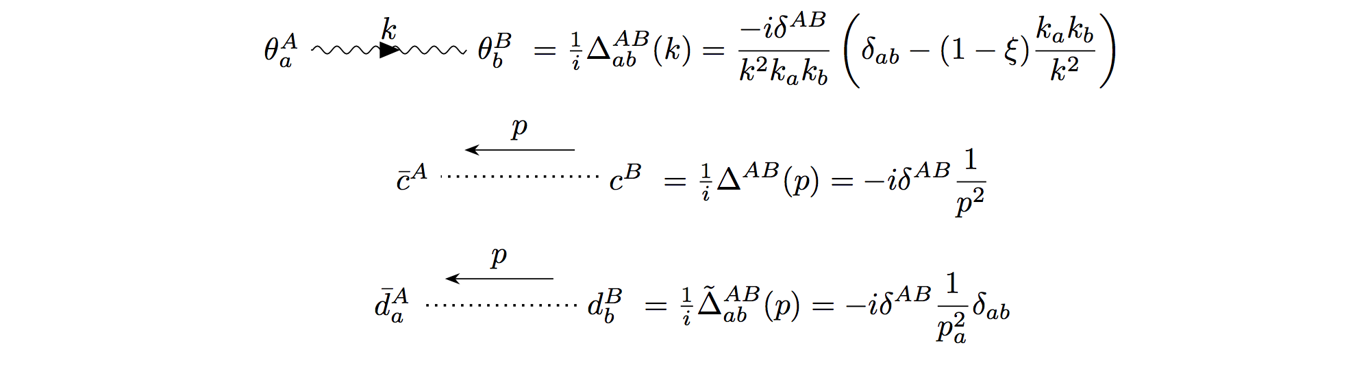
Figure 6: Propagators

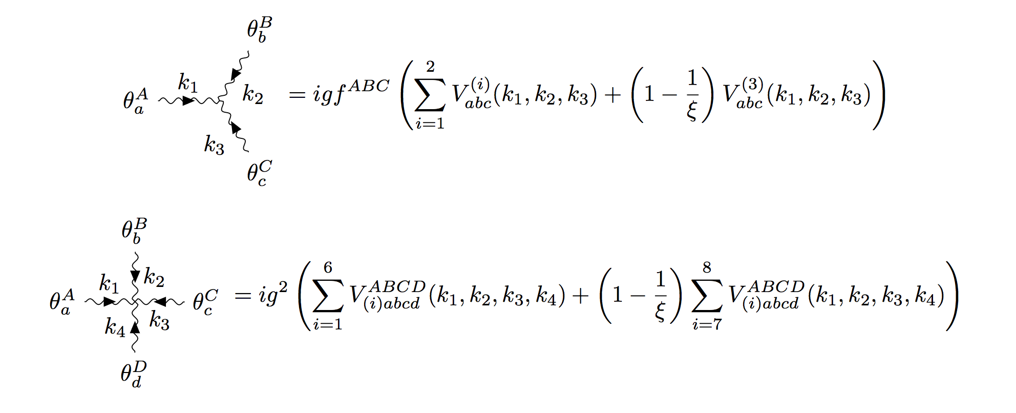
Figure 7: Gauge interaction vertices up to quartic order in $\theta$.

Figure 8: Ghost gauge vertices up to third order in $\theta$

Figure 9: Additional ghost gauge vertices up to second order in $\theta$

Figure 10: Composite operator vertices up to third order in $\theta$

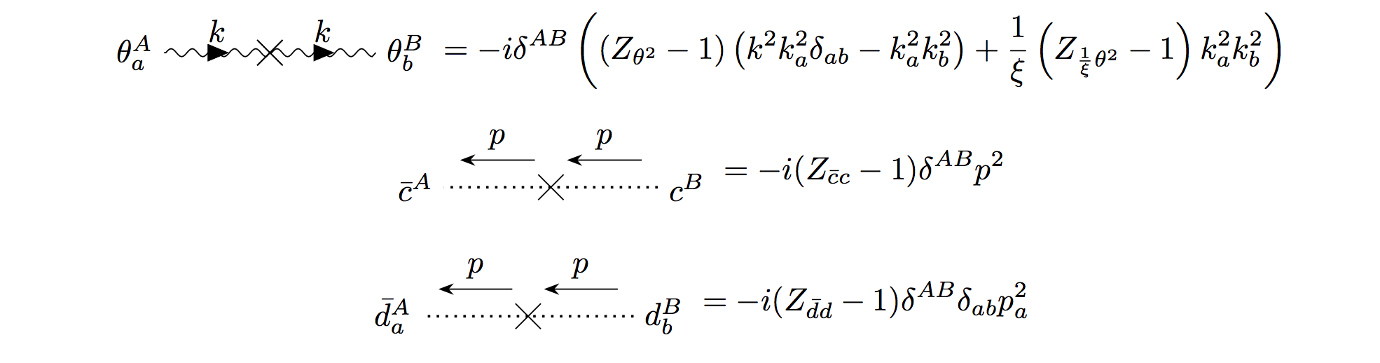
Figure 11: Quadratic counter-terms

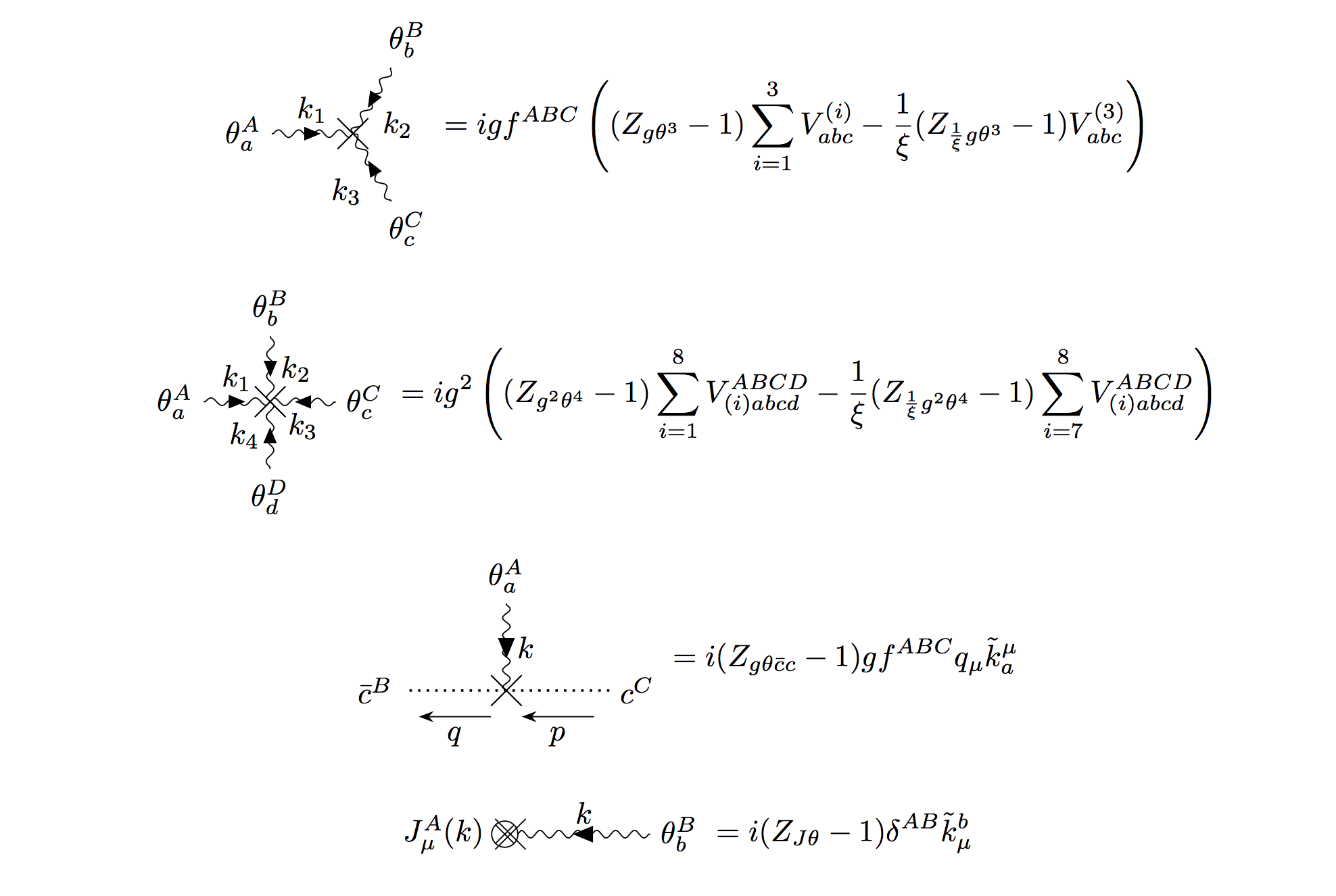
Figure 12: Interaction vertex counter-terms

D.1 Explicit Vertex Expressions

This section contains vertex expressions that were defined in the Feynman rules figures. The $\theta^{3}\bar{c}c$ vertex $V_{abc}^{ABC,DE}\left(k_{1},k_{2},k_{3};q\right)$ defined in Figure 8 is

$$iV_{abc}^{ABC,DE}=\frac{i}{6}\delta_{abc}\tilde{q}_{\mu}^{a}f_{F}^{DE}\left(f_{G}^{FA}f_{G}^{BC}\left(k_{3}^{\mu}-k_{2}^{\mu}\right)+f_{G}^{FB}f_{G}^{CA}\left(k_{1}^{\mu}-k_{3}^{\mu}\right)+f_{G}^{FC}f_{G}^{AB}\left(k_{1}^{\mu}-k_{2}^{\mu}\right)\right),$$ (357)

where the momenta are constrained to satisfy $q=k_{1}+k_{2}+k_{3}+p$. The $\theta^{2}\bar{d}d$ vertex $V_{ab,cd}^{AB,CD}\left(k_{1},k_{2};q,p\right)$ defined in Fig. 9 with $q=k_{1}+k_{2}+p$ is

$$iV_{ab,cd}^{AB,CD}= \frac{i}{6}\delta_{abcd}\tilde{q}_{\mu}^{a}\left(f_{E}^{AB}f_{E}^{CD}(k_{1}^{\mu}-k_{2}^{\mu})+f_{E}^{AC}f_{E}^{BD}(p^{\mu}-k_{2}^{\mu})+f_{E}^{AD}f_{E}^{BC}(p^{\mu}-k_{1}^{\mu})\right).$$ (358)

The $J\theta^{3}$ vertex $V_{\mu,bcd}^{A,BCD}\left(k_{2},k_{3},k_{4}\right)$ defined in Fig. 10 is

$$iV_{\mu,bcd}^{A,BCD}=\frac{i}{6}\delta_{bcd}\left(f_{E}^{AB}f_{E}^{CD}(\tilde{k}_{4\mu}^{b}-\tilde{k}_{3\mu}^{b})+f_{E}^{AC}f_{E}^{BD}(\tilde{k}_{4\mu}^{b}-\tilde{k}_{2\mu}^{b})+f_{E}^{AD}f_{E}^{BC}(\tilde{k}_{3\mu}^{b}-\tilde{k}_{2\mu}^{b})\right),$$ (359)

where the composite operator momentum is $k=-k_{2}-k_{3}-k_{4}$.

D.2 Quartic vertex terms

Here, we are using the notation $\delta_{bcd}=\delta_{bc}\delta_{cd}$ such as to avoid confusion regarding summation. The quartic BTGT gauge vertex in Fig. 7 is given by

$$iV_{abcd}^{ABCD}=ig^{2}\left(\sum_{i=1}^{6}V_{(i)abcd}^{ABCD}\left(k_{1},k_{2},k_{3},k_{4}\right)+\left(1-\tfrac{1}{\xi}\right)\sum_{i=7}^{8}V_{(i)abcd}^{ABCD}\left(k_{1},k_{2},k_{3},k_{4}\right)\right)$$ (360)

where the momenta $k_{i}$ must sum to zero. In a diagonal basis for $H^{a}$, the eight terms are given by

$$V_{(1)abcd}^{ABCD}= -k_{1a}k_{2b}k_{3c}k_{4d}\left(f_{E}^{AB}f_{E}^{CD}\left(\delta_{ac}\delta_{bd}-\delta_{ad}\delta_{bc}\right)+f_{E}^{AC}f_{E}^{BD}\left(\delta_{ab}\delta_{cd}-\delta_{ad}\delta_{bc}\right)\right.$$

$$\left.+f_{E}^{AD}f_{E}^{BC}\left(\delta_{ab}\delta_{cd}-\delta_{ac}\delta_{bd}\right)\right)$$ (361)

$$V_{(2)abcd}^{ABCD}= -\frac{1}{2}\left\{f_{E}^{AB}f_{E}^{CD}\left[\delta_{bcd}k_{1a}\left(k_{3a}+k_{4a}\right)k_{2b}\left(k_{3b}-k_{4b}\right)+\delta_{acd}k_{2b}\left(k_{3b}+k_{4b}\right)k_{1a}\left(k_{4a}-k_{3a}\right)\right.\right.$$

$$\left.+\delta_{abd}k_{3c}\left(k_{1c}+k_{2c}\right)k_{4a}\left(k_{1a}-k_{2a}\right)+\delta_{abc}k_{4d}\left(k_{1d}+k_{2d}\right)k_{3a}\left(k_{2a}-k_{1a}\right)\right]$$

$$+f_{E}^{AC}f_{E}^{BD}\left[\delta_{bcd}k_{1a}\left(k_{2a}+k_{4a}\right)k_{3b}\left(k_{2b}-k_{4b}\right)+\delta_{abd}k_{3c}\left(k_{2c}+k_{4c}\right)k_{1a}\left(k_{4a}-k_{2a}\right)\right.$$

$$\left.+\delta_{acd}k_{2b}\left(k_{1b}+k_{3b}\right)k_{4d}\left(k_{1d}-k_{3d}\right)+\delta_{abc}k_{4\star d}\left(k_{1d}+k_{3d}\right)k_{2b}\left(k_{3b}-k_{1b}\right)\right]$$

$$+f_{E}^{AD}f_{E}^{BC}\left[\delta_{bcd}k_{1a}\left(k_{2a}+k_{3a}\right)k_{4d}\left(k_{2d}-k_{3d}\right)+\delta_{abc}k_{4c}\left(k_{2c}+k_{3c}\right)k_{1a}\left(k_{3a}-k_{2a}\right)\right.$$

$$\left.+\delta_{acd}^{\phantom{A}}\left.k_{2b}\left(k_{1b}+k_{4b}\right)k_{3c}\left(k_{1c}-k_{4c}\right)+\delta_{abd}k_{3c}\left(k_{1c}+k_{4c}\right)k_{2b}\left(k_{4b}-k_{1b}\right)\right]\right\}$$ (362)

$$V_{(3)abcd}^{ABCD}= -\frac{1}{2}\left\{f_{E}^{AB}f_{E}^{CD}\left[\delta_{acd}k_{1b}k_{2b}k_{1a}\left(k_{3a}-k_{4a}\right)+\delta_{bcd}k_{1a}k_{2a}k_{2b}\left(k_{4b}-k_{3b}\right)\right.\right.$$

$$+\left.\delta_{abc}k_{3d}k_{4d}k_{3a}\left(k_{1a}-k_{2a}\right)+\delta_{abd}k_{3c}k_{4c}k_{4a}\left(k_{2a}-k_{1a}\right)\right]$$

$$+f_{E}^{AC}f_{E}^{BD}\left[\delta_{abd}k_{1c}k_{3c}k_{1a}\left(k_{2a}-k_{4a}\right)+\delta_{bcd}k_{1a}k_{3a}k_{3b}\left(k_{4b}-k_{2b}\right)\right.$$

$$\left.+\delta_{abc}k_{2d}k_{4d}k_{2a}\left(k_{1a}-k_{3a}\right)+\delta_{acd}k_{2b}k_{4b}k_{4a}\left(k_{3a}-k_{1a}\right)\right]$$

$$+f_{E}^{AD}f_{E}^{BC}\left[\delta_{abc}k_{1d}k_{4d}k_{1a}\left(k_{2a}-k_{3a}\right)+\delta_{bcd}k_{1a}k_{4a}k_{4b}\left(k_{3b}-k_{2b}\right)\right.$$

$$\left.+\delta_{abd}^{\phantom{A}}\left.k_{2c}k_{3c}k_{2a}\left(k_{1a}-k_{4a}\right)+\delta_{acd}k_{2b}k_{3b}k_{3a}\left(k_{3a}-k_{1a}\right)\right]\right\}$$ (363)

$$V_{(4)abcd}^{ABCD}= \frac{1}{2}\left\{f_{E}^{AB}f_{E}^{CD}\delta_{ab}\delta_{cd}\left[k_{1a}k_{2a}(k_{1c}-k_{2c})(k_{3c}-k_{4c})\right.\right.$$

$$\left.+k_{3c}k_{4c}(k_{1a}-k_{2a})(k_{3a}-k_{4a})\right]$$

$$+f_{E}^{AC}f_{E}^{BD}\delta_{ac}\delta_{bd}\left[k_{1a}k_{3a}\left(k_{1b}-k_{3b}\right)\left(k_{2b}-k_{4b}\right)\right.$$

$$\left.+k_{2b}k_{4b}\left(k_{1a}-k_{3a}\right)\left(k_{2a}-k_{4a}\right)\right]$$

$$+f_{E}^{AD}f_{E}^{CD}\delta_{ad}\delta_{bc}\left[k_{1a}k_{4a}(k_{1b}-k_{4b})(k_{2b}-k_{3b})\right.$$

$$\left.+k_{2b}^{\phantom{A}}\left.k_{3b}(k_{1a}-k_{4a})(k_{2a}-k_{3a})\right]\right\}$$ (364)

$$V_{(5)abcd}^{ABCD}= \frac{1}{4}\delta_{abcd}\left\{f_{E}^{AB}f_{E}^{CD}\left(k_{1}+k_{2}\right)^{2}\left(k_{1a}-k_{2a}\right)\left(k_{3a}-k_{4a}\right)\right.$$

$$+f_{E}^{AC}f_{E}^{BD}\left(k_{1}+k_{3}\right)^{2}\left(k_{1a}-k_{3a}\right)\left(k_{2a}-k_{4a}\right)$$

$$\left.+f_{E}^{AD}f_{E}^{BC}\left(k_{1}+k_{4}\right)^{2}\left(k_{1a}-k_{4a}\right)\left(k_{2a}-k_{3a}\right)\right\}$$ (365)

$$V_{(6)abcd}^{ABCD}= \frac{1}{6}\delta_{abcd}\left\{f_{E}^{AB}f_{E}^{CD}\left[\left(k_{1}^{2}k_{1a}-k_{2}^{2}k_{2a}\right)\left(k_{4a}-k_{3a}\right)+\left(k_{3}^{2}k_{3a}-k_{4}^{2}k_{4a}\right)\left(k_{2a}-k_{1a}\right)\right]\right.$$

$$+f_{E}^{AC}f_{E}^{BD}\left[\left(k_{1}^{2}k_{1a}-k_{3}^{2}k_{3a}\right)\left(k_{4a}-k_{2a}\right)+\left(k_{2}^{2}k_{2a}-k_{4}^{2}k_{4a}\right)\left(k_{3a}-k_{1a}\right)\right]$$

$$\left.+f_{E}^{AD}f_{E}^{BC}\left[\left(k_{1}^{2}k_{1a}-k_{4}^{2}k_{4a}\right)\left(k_{3a}-k_{2a}\right)+\left(k_{2}^{2}k_{2a}-k_{3}^{2}k_{3a}\right)\left(k_{4a}-k_{1a}\right)\right]\right\}$$ (366)

$$V_{(7)abcd}^{ABCD}= -\frac{1}{4}\left\{f_{E}^{AB}f_{E}^{CD}\delta_{ab}\delta_{cd}\left(k_{1a}-k_{2a}\right)\left(k_{1a}+k_{2a}\right)\left(k_{3c}-k_{4c}\right)\left(k_{1c}+k_{2c}\right)\right.$$

$$+f_{E}^{AC}f_{E}^{BD}\delta_{ac}\delta_{bd}\left(k_{1a}-k_{3a}\right)\left(k_{1a}+k_{3a}\right)\left(k_{2b}-k_{4b}\right)\left(k_{1b}+k_{3b}\right)$$

$$+\left.f_{E}^{AD}f_{E}^{BC}\delta_{ad}\delta_{bc}\left(k_{1a}-k_{4a}\right)\left(k_{1a}+k_{4a}\right)\left(k_{2b}-k_{3b}\right)\left(k_{1b}+k_{4b}\right)\right\}$$ (367)

$$V_{(8)abcd}^{ABCD}= -\frac{1}{6}\left\{f_{E}^{AB}f_{E}^{CD}\left[\delta_{bcd}k_{1a}^{2}k_{1b}\left(k_{4b}-k_{3b}\right)+\delta_{acd}k_{2b}^{2}k_{2a}\left(k_{3a}-k_{4a}\right)\right.\right.$$

$$\left.+\delta_{abd}k_{3c}^{2}k_{3a}\left(k_{2a}-k_{1a}\right)+\delta_{abc}k_{4d}^{2}k_{4a}\left(k_{1a}-k_{2a}\right)\right]$$

$$+f_{E}^{AC}f_{E}^{BD}\left[\delta_{bcd}k_{1a}^{2}k_{1b}\left(k_{4b}-k_{2b}\right)+\delta_{abd}k_{3c}^{2}k_{3a}\left(k_{2a}-k_{4a}\right)\right.$$

$$+\left.\delta_{acd}k_{2b}^{2}k_{2a}\left(k_{3a}-k_{1a}\right)+\delta_{abc}k_{4d}^{2}k_{4a}\left(k_{1a}-k_{3a}\right)\right]$$

$$+f_{E}^{AD}f_{E}^{BC}\left[\delta_{bcd}k_{1a}^{2}k_{1b}\left(k_{3b}-k_{2b}\right)+\delta_{abc}k_{4d}^{2}k_{4a}\left(k_{2a}-k_{3a}\right)\right.$$

$$\left.+\delta_{acd}^{\phantom{A}}\left.k_{2b}^{2}k_{2a}\left(k_{4a}-k_{1a}\right)+\delta_{abd}k_{3c}^{2}k_{3a}\left(k_{1a}-k_{4a}\right)\right]\right\}\,\,.$$ (368)

References

- (1) S. L. Glashow, Partial Symmetries of Weak Interactions, Nucl. Phys. 22 (1961) 579–588.
- (2) S. Weinberg, A Model of Leptons, Phys. Rev. Lett. 19 (1967) 1264–1266.
- (3) A. Salam, Weak and Electromagnetic Interactions, Conf. Proc. C680519 (1968) 367–377.
- (4) D. J. Gross and F. Wilczek, Ultraviolet Behavior of Nonabelian Gauge Theories, Phys. Rev. Lett. 30 (1973) 1343–1346.
- (5) H. D. Politzer, Reliable Perturbative Results for Strong Interactions?, Phys. Rev. Lett. 30 (1973) 1346–1349.
- (6) S. Weinberg, The quantum theory of fields. Vol. 2: Modern applications. Cambridge University Press, 2013.
- (7) P. Ramond, Journeys beyond the standard model, Front. Phys. 101 (1999) 1–390.
- (8) P. Langacker, The standard model and beyond. 2010.
- (9) ATLAS collaboration, G. Aad et al., Observation of a new particle in the search for the Standard Model Higgs boson with the ATLAS detector at the LHC, Phys. Lett. B716 (2012) 1–29, [1207.7214].
- (10) CMS collaboration, S. Chatrchyan et al., Observation of a new boson at a mass of 125 GeV with the CMS experiment at the LHC, Phys. Lett. B716 (2012) 30–61, [1207.7235].
- (11) M. Nakahara, Geometry, topology and physics. 2003.
- (12) T. T. Wu and C. N. Yang, Concept of Nonintegrable Phase Factors and Global Formulation of Gauge Fields, Phys. Rev. D12 (1975) 3845–3857.
- (13) H. Weyl, A New Extension of Relativity Theory, Annalen Phys. 59 (1919) 101–133.
- (14) H. Weyl, Electron and Gravitation. 1. (In German), Z. Phys. 56 (1929) 330–352.
- (15) C.-N. Yang and R. L. Mills, Conservation of Isotopic Spin and Isotopic Gauge Invariance, Phys. Rev. 96 (1954) 191–195.
- (16) E. S. Abers and B. W. Lee, Gauge Theories, Phys. Rept. 9 (1973) 1–141.
- (17) C. Itzykson and J. B. Zuber, Quantum Field Theory. International Series In Pure and Applied Physics. McGraw-Hill, New York, 1980.
- (18) A. M. Polyakov, Gauge Fields and Strings, Contemp. Concepts Phys. 3 (1987) 1–301.
- (19) G. F. Sterman, An Introduction to quantum field theory. Cambridge University Press, 1993.
- (20) G. ’t Hooft, Under the spell of the gauge principle, Adv. Ser. Math. Phys. 19 (1994) 1–683.
- (21) N. Arkani-Hamed and J. Trnka, The Amplituhedron, JHEP 10 (2014) 030, [1312.2007].
- (22) N. Arkani-Hamed, T.-C. Huang and Y.-t. Huang, Scattering Amplitudes For All Masses and Spins, 1709.04891.
- (23) S. D. Badger, E. W. N. Glover, V. V. Khoze and P. Svrcek, Recursion relations for gauge theory amplitudes with massive particles, JHEP 07 (2005) 025, [hep-th/0504159].
- (24) H. Elvang and Y.-t. Huang, Scattering Amplitudes, 1308.1697.
- (25) J. M. Henn and J. C. Plefka, Scattering Amplitudes in Gauge Theories, Lect. Notes Phys. 883 (2014) pp.1–195.
- (26) N. Christensen and B. Field, Constructive standard model, Phys. Rev. D98 (2018) 016014, [1802.00448].
- (27) E. Witten, Anti-de Sitter space and holography, Adv. Theor. Math. Phys. 2 (1998) 253–291, [hep-th/9802150].
- (28) O. Aharony, S. S. Gubser, J. M. Maldacena, H. Ooguri and Y. Oz, Large N field theories, string theory and gravity, Phys. Rept. 323 (2000) 183–386, [hep-th/9905111].
- (29) D. J. H. Chung and R. Lu, Basis tensor gauge theory: Reformulating gauge theories with basis tensor fields, Phys. Rev. D94 (2016) 105016, [1609.03679].
- (30) K. G. Wilson, Confinement of Quarks, Phys. Rev. D10 (1974) 2445–2459.
- (31) R. Giles, The Reconstruction of Gauge Potentials From Wilson Loops, Phys. Rev. D24 (1981) 2160.
- (32) A. A. Migdal, Loop Equations and 1/N Expansion, Phys. Rept. 102 (1983) 199–290.
- (33) J. Terning, Gauging nonlocal Lagrangians, Phys. Rev. D44 (1991) 887–897.
- (34) D. J. Gross, A. Hashimoto and N. Itzhaki, Observables of noncommutative gauge theories, Adv. Theor. Math. Phys. 4 (2000) 893–928, [hep-th/0008075].
- (35) A. Kapustin, Wilson-’t Hooft operators in four-dimensional gauge theories and S-duality, Phys. Rev. D74 (2006) 025005, [hep-th/0501015].
- (36) I. O. Cherednikov and N. G. Stefanis, Wilson lines and transverse-momentum dependent parton distribution functions: A Renormalization-group analysis, Nucl. Phys. B802 (2008) 146–179, [0802.2821].
- (37) S. Mandelstam, Quantum electrodynamics without potentials, Annals Phys. 19 (1962) 1–24.
- (38) D. J. H. Chung, Ward Identity and Basis Tensor Gauge Theory at One Loop, Phys. Rev. D97 (2018) 125003, [1712.10118].
- (39) R. P. Woodard, Avoiding dark energy with 1/r modifications of gravity, Lect. Notes Phys. 720 (2007) 403–433, [astro-ph/0601672].
- (40) S. W. Hawking and T. Hertog, Living with ghosts, Phys. Rev. D65 (2002) 103515, [hep-th/0107088].
- (41) I. Antoniadis, E. Dudas and D. M. Ghilencea, Living with ghosts and their radiative corrections, Nucl. Phys. B767 (2007) 29–53, [hep-th/0608094].
- (42) T.-j. Chen, M. Fasiello, E. A. Lim and A. J. Tolley, Higher derivative theories with constraints: Exorcising Ostrogradski’s Ghost, JCAP 1302 (2013) 042, [1209.0583].
- (43) A. Salvio and A. Strumia, Quantum mechanics of 4-derivative theories, Eur. Phys. J. C76 (2016) 227, [1512.01237].
- (44) A. Grozin, Lectures on QED and QCD, in 3rd Dubna International Advanced School of Theoretical Physics Dubna, Russia, January 29-February 6, 2005, pp. 1–156, 2005, hep-ph/0508242.
- (45) L. F. Alday and R. Roiban, Scattering Amplitudes, Wilson Loops and the String/Gauge Theory Correspondence, Phys. Rept. 468 (2008) 153–211, [0807.1889].
- (46) G. P. Korchemsky and G. Marchesini, Structure function for large x and renormalization of Wilson loop, Nucl. Phys. B406 (1993) 225–258, [hep-ph/9210281].
- (47) G. P. Korchemsky and A. V. Radyushkin, Infrared factorization, Wilson lines and the heavy quark limit, Phys. Lett. B279 (1992) 359–366, [hep-ph/9203222].
- (48) J. Frenkel and J. C. Taylor, NONABELIAN EIKONAL EXPONENTIATION, Nucl. Phys. B246 (1984) 231–245.
- (49) S. Catani and M. Ciafaloni, Many Gluon Correlations and the Quark Form-factor in QCD, Nucl. Phys. B236 (1984) 61–89.
- (50) A. S. Kronfeld, Twenty-first Century Lattice Gauge Theory: Results from the QCD Lagrangian, Ann. Rev. Nucl. Part. Sci. 62 (2012) 265–284, [1203.1204].
- (51) N. Brambilla et al., QCD and Strongly Coupled Gauge Theories: Challenges and Perspectives, Eur. Phys. J. C74 (2014) 2981, [1404.3723].
- (52) E. Witten, Global Aspects of Current Algebra, Nucl. Phys. B223 (1983) 422–432.
- (53) D. Gaiotto, A. Kapustin, N. Seiberg and B. Willett, Generalized Global Symmetries, JHEP 02 (2015) 172, [1412.5148].
- (54) J. Ellis, TikZ-Feynman: Feynman diagrams with TikZ, Comput. Phys. Commun. 210 (2017) 103–123, [1601.05437].