Projection factors and generalized real and complex Pythagorean theorems

Abstract

Projection factors describe the contraction of Lebesgue measures in orthogonal projections between subspaces of a real or complex inner product space. They are connected to Grassmann’s exterior algebra and the Grassmann angle between subspaces, and lead to generalized Pythagorean theorems, relating measures of subsets of real or complex subspaces and their orthogonal projections on certain families of subspaces.

The complex Pythagorean theorems differ from the real ones in that the measures are not squared, and this may have important implications for quantum theory. Projection factors of the complex line of a quantum state with the eigenspaces of an observable give the corresponding quantum probabilities. The complex Pythagorean theorem for lines corresponds to the condition of unit total probability, and may provide a way to solve the probability problem of Everettian quantum mechanics.

Keywords: projection factor, Pythagorean theorem, Grassmann algebra, Grassmann angle, quantum mechanics

MSC: 51M05, 28A75, 15A75, 81P16

1 Introduction

The importance of the Pythagorean theorem is reflected in its many generalizations. One which is well known, playing an essential role in quantum mechanics, is that if $X=\bigoplus_{i\in\mathcal{I}}V_{i}$ is a partition of a real or complex Hilbert space $X$ into a family $\{V_{i}\}_{i\in\mathcal{I}}$ of mutually orthogonal closed subspaces, and $P_{i}$ is the orthogonal projection on $V_{i}$, then for any $v\in X$,

$$\|v\|^{2}=\sum\limits_{i\in\mathcal{I}}\left\|P_{i}v\right\|^{2}.$$ (1)

Less known generalizations, which keep being rediscovered time and again, relate areas, volumes or Lebesgue measures in general to their orthogonal projections [AMB96, Atz00, CB74, DC35, Dru15]. They are usually proven for parallelotopes or simplices, using determinant identities such as the Cauchy-Binet formula [Gan00], being sometimes extended to other figures via integral calculus or measure theory. There is even a neat proof via divergence theorem [ER08].

Using projection factors, which describe the contraction of Lebesgue measures under orthogonal projections, we reobtain these generalizations, with much simpler proofs, and extend them to complex vector spaces. This is done by relating these factors to Grassmann’s exterior algebra [Win10, Yok92]. Many useful properties are also obtained by connecting them to the Grassmann angle between subspaces [Man19a, Man19b].

An unusual feature of the complex Pythagorean theorems is that measures are not squared (which is compensated by their dimensions being doubled), and this may allow projection factors to play a fundamental role in quantum mechanics. In the Hilbert space of a quantum system, the projection factors of the complex line of a quantum state with the eigenspaces of an observable equal the corresponding quantum probabilities. And the total probability being 1 corresponds to the complex Pythagorean theorem for lines. In [Man19c] we show this can be used to obtain the Born rule in Everettian quantum mechanics, i.e. the many-worlds interpretation [EI57, SBKW10].

In sc:projection factors we study projection factors, and relate them to the Grassmann algebra. The generalized Pythagorean theorems are obtained in sc:Pythagorean thms, and sc:epilogue closes with a few remarks. In sc:Properties of projection factors we list other useful properties of projection factors.

2 Projection factors

Let $X$ be a $n$-dimensional vector space over $\mathds{R}$ (real case) or $\mathds{C}$ (complex case), with inner product $\langle\cdot,\cdot\rangle$ (Hermitian product in the complex case). Unless otherwise indicated, whenever we refer to subspaces or other linear algebra concepts of $X$, it will be with respect to the same field as $X$.

Complex vector spaces can also be seen as real ones, with twice the complex dimension, and the real part of a Hermitian product $\langle\cdot,\cdot\rangle$ gives a real inner product $\operatorname{Re}\langle\cdot,\cdot\rangle$ in the underlying real vector space. As $\mathds{C}$-orthogonality (with respect to $\langle\cdot,\cdot\rangle$) implies $\mathds{R}$-orthogonality (with respect to $\operatorname{Re}\langle\cdot,\cdot\rangle$), orthogonal projections with respect to both products coincide.

On any real or complex subspace $V\subset X$, let $|\cdot|_{m}$ be the $m$-dimensional Lebesgue measure if $m=\dim_{\mathds{R}}V$, and $|\!\cdot\!|_{m}=0$ if $m>\dim_{\mathds{R}}V$.

Definition.

For subspaces $V,W\subset X$, let $P:V\rightarrow W$ be the orthogonal projection and $p=\dim_{\mathds{R}}V$. The projection factor of $V$ on $W$ is

$$\pi_{V,W}=\frac{|P(S)|_{p}}{|S|_{p}},$$

where $S$ is any Lebesgue measurable subset of $V$ with $|S|_{p}\neq 0$.

Remark 1.

$|P(S)|_{p}$ is defined, since $\dim_{\mathds{R}}P(V)\leq p$.

Remark 2.

As $P$ is linear, $\pi_{V,W}$ does not depend on $S$. More precisely, $\pi_{V,W}=0$ if $\dim_{\mathds{R}}P(V)<p$, and if $\dim_{\mathds{R}}P(V)=p$ then $V$ and $P(V)$ can be isometrically identified with $\mathds{R}^{p}$, in which case independence of $S$ is a defining property of the Lebesgue measure [Rud86, p.51].

Clearly, the projection factor for complex subspaces equals that of their underlying real vector spaces. Also, $\pi_{V,W}$ depends only on the relative position of $V$ and $W$, being invariant by any orthogonal transformation $T$ (unitary, in the complex case), as $T$ preserves Lebesgue measures and the orthogonal projection of $T(S)$ on $T(W)$ coincides with $T(P(S))$.

Calculations will be simpler when $S$ is a parallelotope.

Definition.

The parallelotope spanned by $v_{1},\ldots,v_{k}\in X$ is

$$[v_{1},\ldots,v_{k}]=\{t_{1}v_{1}+\ldots+t_{k}v_{k}:t_{1},\ldots,t_{k}\in[0,1]\}.$$

The parallelotope is orthogonal if the $v_{i}$’s are mutually $\mathds{R}$-orthogonal, in which case $\big{|}[v_{1},\ldots,v_{k}]\big{|}_{k}=\|v_{1}\|\cdot\ldots\cdot\|v_{k}\|$. If $P$ is the orthogonal projection onto a subspace $W\subset X$ then

$$P([v_{1},\ldots,v_{k}])=[Pv_{1},\ldots,Pv_{k}].$$

2.1 Projection factors of lines

Definition.

For any $v\in X$, let $\mathds{R}v=\{cv:c\in\mathds{R}\}$, and in the complex case also $\mathds{C}v=\{cv:c\in\mathds{C}\}$.

Definition.

A line $L\subset X$ is a 1-dimensional subspace. A nonzero $v\in X$ determines a real line $\mathds{R}v$ (in the complex case, it should be understood as a subspace of the underlying real vector space), and in the complex case also a complex line $\mathds{C}v$ (which is isometric to a real plane).

Proposition 2.1.

Given $v\in X$ and a real or complex subspace $W\subset X$, let $P$ be the orthogonal projection on $W$. Then

$$\|Pv\|=\|v\|\cdot\pi_{\mathds{R}v,W}.$$

In the complex case, with $W$ being a complex subspace, we also have

$$\|Pv\|^{2}=\|v\|^{2}\cdot\pi_{\mathds{C}v,W}.$$ (2)

Proof.

The first identity follows from the definition, and the other from the fact that orthogonal projections onto complex subspaces are $\mathds{C}$-linear, so the square $[v,\mathrm{i}v]\subset\mathds{C}v$ projects to the square $[Pv,\mathrm{i}Pv]$. ∎

In sc:Properties of projection factors we give more general formulas (pr:properties pi xiv).

Example 2.2.

Let $X$ be the Hilbert space of a quantum system, $\mathds{C}\psi$ be the complex line of a quantum state $\psi$ (its ray, except for the origin), and $W$ be the eigenspace of a quantum observable corresponding to some eigenvalue $\lambda$. By (2), $\pi_{\mathds{C}\psi,W}$ equals the probability of obtaining $\lambda$ when measuring $\psi$ for that observable. In [Man19c] we explore this relation between projection factors and quantum probabilities.

Proposition 2.3.

For any $v,w\in X$, we have:

• In the real case, $|\langle v,w\rangle|=\|v\|\|w\|\cdot\pi_{\mathds{R}v,\mathds{R}w}$.

• In the complex case,

  $$|\operatorname{Re}\langle v,w\rangle| =\|v\|\|w\|\cdot\pi_{\mathds{R}v,\mathds{R}w},$$

  $$|\langle v,w\rangle| =\|v\|\|w\|\cdot\pi_{\mathds{R}v,\mathds{C}w},$$

  $$|\langle v,w\rangle|^{2} =\|v\|^{2}\|w\|^{2}\cdot\pi_{\mathds{C}v,\mathds{C}w}.$$ (3)

Proof.

Follows from pr:Pv pi, as the orthogonal projection of $v$ on $W=\mathds{R}w$ (real case, or underlying real space in the complex one) or $W=\mathds{C}w$ (complex case) is $Pv=\frac{\langle w,v\rangle}{\|w\|^{2}}w$. ∎

Projection factors between lines clearly depend on the angle between them. But some care is needed in the complex case, as there are different concepts of angle between complex vectors [GH06, Sch01].

Definition.

The Euclidean angle $\theta_{v,w}\in[0,\pi]$ of nonzero vectors $v,w\in X$ is the usual angle between them, considered as real vectors, i.e.

$$\cos\theta_{v,w}=\frac{\operatorname{Re}\langle v,w\rangle}{\|v\|\|w\|}.$$

In the complex case, the Hermitian angle $\gamma_{v,w}\in[0,\frac{\pi}{2}]$ is defined by

$$\cos\gamma_{v,w}=\dfrac{|\langle v,w\rangle|}{\|v\|\|w\|}.$$

The Hermitian angle is the (Euclidean) angle between $v$ and the plane $\mathds{C}w$, and gives the Fubini-Study distance between the lines $\mathds{C}v$ and $\mathds{C}w$ in the complex projective space $\mathds{P}(X)$.

Corollary 2.4.

For any nonzero vectors $v,w\in X$,

$$\pi_{\mathds{R}v,\mathds{R}w}=\left|\cos\theta_{v,w}\right|.$$

Also, in the complex case,

$$\pi_{\mathds{R}v,\mathds{C}w} =\cos\gamma_{v,w},$$

$$\pi_{\mathds{C}v,\mathds{C}w} =\cos^{2}\gamma_{v,w}.$$

Example 2.5.

By (3), the fidelity [BŻ17] of pure quantum states $\psi$ and $\varphi$ equals $\pi_{\mathds{C}\psi,\mathds{C}\varphi}$, and their Bures angle is the same as $\gamma_{\psi,\varphi}$.

2.2 Principal projection factors

Let $V,W\subset X$ be nonzero subspaces, $p=\dim V$, $q=\dim W$, and $m=\min\{p,q\}$. A singular value decomposition gives [GH06] orthonormal principal bases $(e_{1},\ldots,e_{p})$ of $V$ and $(f_{1},\ldots,f_{q})$ of $W$ in which the orthogonal projection $P:V\rightarrow W$ is given by a $q\times p$ diagonal matrix $\mathbf{P}$ with real non-negative diagonal elements $1\geq\sigma_{1}\geq\ldots\geq\sigma_{m}\geq 0$, its singular values. The $e_{i}$’s and $f_{j}$’s are principal vectors of $V$ and $W$, and satisfy

$$\langle e_{i},f_{j}\rangle=\begin{cases}0\hskip 7.0pt\text{ if }i\neq j,\\ \sigma_{i}\ \text{ if }i=j.\end{cases}$$ (4)

This has a nice geometric interpretation. The unit sphere of $V$ projects to an ellipsoid in $W$. In the real case, for $1\leq i\leq m$, the $\sigma_{i}$’s are the lengths of its semi-axes, the $e_{i}$’s project onto them, and the $f_{i}$’s point along them. In the complex case, for each $1\leq i\leq m$ there are two semi-axes of length $\sigma_{i}$, corresponding to the projections of $e_{i}$ and $\mathrm{i}e_{i}$.

It also admits a variational characterization, given recursively as follows. For each $i=1,\ldots,m$, let

$$\begin{cases}V_{i}=\{v\in V:\langle v,e_{j}\rangle=0\ \forall\,j<i\},\\ W_{i}=\{w\in W:\langle w,f_{j}\rangle=0\ \forall\,j<i\},\\ \sigma_{i}=\max\left\{\,|\langle v,w\rangle|:v\in V_{i},w\in W_{i},\|v\|=\|w\|=1\right\},\\ e_{i}\in V_{i},f_{i}\in W_{i}\text{ are unit vectors such that }\langle e_{i},f_{i}\rangle=\sigma_{i}.\end{cases}$$

Definition.

For $1\leq i\leq m$, the principal projection factor $\pi_{i}$ of $V$ and $W$ is the projection factor for the lines of $e_{i}$ and $f_{i}$, i.e.

$$\pi_{i}=\begin{cases}\pi_{\mathds{R}e_{i},\mathds{R}f_{i}}\,\text{ in the real case,}\\ \pi_{\mathds{C}e_{i},\mathds{C}f_{i}}\ \text{ in the complex case.}\end{cases}$$

From pr:product projection factor and (4) we get, for $1\leq i\leq m$,

$$\pi_{i}=\begin{cases}\sigma_{i}\ \,\text{ in the real case,}\\ \sigma_{i}^{2}\ \text{ in the complex case.}\end{cases}$$ (5)

Theorem 2.6.

For nonzero subspaces $V,W\subset X$,

$$\pi_{V,W}=\begin{cases}\pi_{1}\cdot\ldots\cdot\pi_{p}\ \text{ if }\dim V=p\leq\dim W,\\ 0\hskip 42.67912pt\text{ if }\dim V>\dim W,\end{cases}$$

where the $\pi_{i}$’s are their principal projection factors.

Proof.

If $\dim V>\dim W$ then $|P(S)|_{p}=0$ by definition. Otherwise,

• in the real case, $S=[e_{1},\ldots,e_{p}]$ is a hypercube with $|S|_{p}=1$ and $P(S)=[\sigma_{1}f_{1},\ldots,\sigma_{p}f_{p}]$ is an orthogonal parallelotope with $|P(S)|_{p}=\sigma_{1}\cdot\ldots\cdot\sigma_{p}=\pi_{1}\cdot\ldots\cdot\pi_{p}$;

• in the complex case, $S=[e_{1},\mathrm{i}e_{1},\ldots,e_{p},\mathrm{i}e_{p}]$ is a hypercube with $|S|_{2p}=1$ and $P(S)=[\sigma_{1}f_{1},\mathrm{i}\sigma_{1}f_{1},\ldots,\sigma_{p}f_{p},\mathrm{i}\sigma_{p}f_{p}]$ is an orthogonal parallelotope with $|P(S)|_{2p}=\sigma^{2}_{1}\cdot\ldots\cdot\sigma^{2}_{p}=\pi_{1}\cdot\ldots\cdot\pi_{p}$. ∎

So, in the real case, the factor by which $p$-dimensional volumes in $V$ shrink when projecting onto $W$ is the product of the factors by which lengths in the principal lines $\mathds{R}e_{i}$ contract. In the complex case, the factor by which $2p$-dimensional volumes in $V$ shrink is the product of the factors by which areas in the principal complex lines $\mathds{C}e_{i}$ contract.

We now give practical formulas for computing $\pi_{V,W}$ in terms of orthonormal bases. In pr:formula general bases we extend them to other bases.

Proposition 2.7.

Let $V,W\subset X$ be nonzero subspaces, and $\mathbf{P}$ be a matrix representing the orthogonal projection $P:V\rightarrow W$ in orthonormal bases of $V$ and $W$. Then

$$\pi_{V,W}=\begin{cases}\sqrt{\det\left(\mathbf{P}^{T}\mathbf{P}\right)}\,\text{ in the real case,}\\ \hskip 6.0pt\det\left(\bar{\mathbf{P}}^{T}\mathbf{P}\right)\hskip 2.0pt\text{ in the complex case.}\end{cases}$$

If $\dim V=\dim W$ then

$$\pi_{V,W}=\begin{cases}|\det\mathbf{P}|\hskip 4.0pt\text{ in the real case,}\\ |\det\mathbf{P}|^{2}\text{ in the complex case.}\end{cases}$$

Proof.

It is enough to consider principal bases of $V$ and $W$, for which $\mathbf{P}$ is a diagonal matrix with the $\sigma_{i}$’s in the diagonal. Then the result follows from (5) and pr:projection factors. ∎

Principal projection factors are directly connected to Jordan’s principal or canonical angles [GH06, Glu67, Wed83].

Definition.

The principal angles $0\leq\theta_{1}\leq\ldots\leq\theta_{m}\leq\frac{\pi}{2}$ of $V$ and $W$ are the angles $\theta_{i}=\theta_{e_{i},f_{i}}$ between their principal vectors.

As $\langle e_{i},f_{i}\rangle\geq 0$, in the complex case we also have $\theta_{i}=\gamma_{e_{i},f_{i}}$.

By (4), $\sigma_{i}=\cos\theta_{i}$, so that, for $1\leq i\leq m$,

$$\pi_{i}=\begin{cases}\cos\theta_{i}\ \,\text{ in the real case,}\\ \cos^{2}\theta_{i}\text{ in the complex case.}\end{cases}$$ (6)

2.3 Grassmann algebra and Grassmann angle

The full power of projection factors is unleashed by connecting them to Grassmann’s exterior algebra [SKM89, Win10, Yok92].

A ($p$-)blade is a decomposable $p$-vector $\nu=v_{1}\wedge\ldots\wedge v_{p}\in\Lambda^{p}X$. The inner product (Hermitian, in the complex case) in the exterior power $\Lambda^{p}X$ is defined by extending linearly (sesquilinearly, in the complex case) the following formula for $p$-blades $\nu=v_{1}\wedge\ldots\wedge v_{p}$ and $\omega=w_{1}\wedge\ldots\wedge w_{p}$:

$$\langle\nu,\omega\rangle=\det\big{(}\langle v_{i},w_{j}\rangle\big{)}=\begin{vmatrix}\langle v_{1},w_{1}\rangle&\cdots&\langle v_{1},w_{p}\rangle\\ \vdots&\ddots&\vdots\\ \langle v_{p},w_{1}\rangle&\cdots&\langle v_{p},w_{p}\rangle\end{vmatrix}.$$

The norm $\|\nu\|=\sqrt{\langle\nu,\nu\rangle}$ of a $p$-blade $\nu=v_{1}\wedge\ldots\wedge v_{p}$ gives, in the real case, the $p$-dimensional volume of $[v_{1},\ldots,v_{p}]$. In the complex case, its square gives the $2p$-dimensional volume of $[v_{1},\mathrm{i}v_{1},\ldots,v_{p},\mathrm{i}v_{p}]$.

Theorem 2.8.

If $\dim V=\dim W=p$ then, for any nonzero blades $\nu\in\Lambda^{p}V$ and $\omega\in\Lambda^{p}W$,

$$\pi_{V,W}=\begin{cases}\hskip 2.0pt\frac{|\langle\nu,\omega\rangle|}{\|\nu\|\|\omega\|}\hskip 11.0pt\text{in the real case},\\[3.0pt] \frac{|\langle\nu,\omega\rangle|^{2}}{\|\nu\|^{2}\|\omega\|^{2}}\,\text{ in the complex case}.\end{cases}$$

Proof.

As $\dim\Lambda^{p}V=\dim\Lambda^{p}W=1$, it is enough to consider unit $p$-blades $\nu=e_{1}\wedge\ldots\wedge e_{p}$ and $\omega=f_{1}\wedge\ldots\wedge f_{p}$ formed with principal vectors of $V$ and $W$. Then (4) gives $\langle\nu,\omega\rangle=\sigma_{1}\cdot\ldots\cdot\sigma_{p}$, and the result follows from (5) and pr:projection factors. ∎

So, for subspaces of same dimension, $\pi_{V,W}$ is related to the inner product of blades. In sc:Properties of projection factors, similar formulas show that for different dimensions it is related to the interior product (pr:properties pi xv), and $\pi_{V,W^{\perp}}$ is related to the exterior product (pr:properties pi perp v).

A line $L$ forms with a subspace $W$ a single principal angle, which is simply called the angle $\theta_{L,W}$ between them. In this case, pr:projection factors turns (6) into

$$\pi_{L,W}=\begin{cases}\cos\theta_{L,W}\ \,\text{ in the real case,}\\ \cos^{2}\theta_{L,W}\text{ in the complex case.}\end{cases}$$ (7)

Extending this to arbitrary subspaces requires an appropriate concept of angle between subspaces, as in high dimensions there are several distinct ones, such as minimal angle [Dix49], Friedrichs angle [Fri37], and others. The reason for such diversity is that the whole list of principal angles is needed to fully describe the relative position of two subspaces [Won67].

Definition.

Let $V,W\subset X$ be nonzero subspaces, $p=\dim V$ and $q=\dim W$. The Grassmann angle $\Theta_{V,W}\in[0,\frac{\pi}{2}]$ of $V$ with $W$ is

$$\Theta_{V,W}=\begin{cases}\arccos(\cos\theta_{1}\cdot\ldots\cdot\cos\theta_{p})\ \text{ if }p\leq q,\\ \frac{\pi}{2}\hskip 97.0pt\text{ if }p>q,\end{cases}$$

where the $\theta_{i}$’s are the principal angles of $V$ and $W$. We also define $\Theta_{\{0\},\{0\}}=\Theta_{\{0\},W}=0$ and $\Theta_{V,\{0\}}=\frac{\pi}{2}$.

This angle was introduced in [Man19a], unifying and extending other angle concepts found in the literature [Glu67, GNSB05, Hit10, Jia96]. It has many interesting properties, and some strange features, which derive from the fact that $\Theta_{V,W}$ is actually an angle in the exterior power $\Lambda^{p}X$, where $p=\dim V$, between the line $\Lambda^{p}V$ and the subspace $\Lambda^{p}W$,

$$\Theta_{V,W}=\theta_{\Lambda^{p}V,\Lambda^{p}W}.$$ (8)

Theorem 2.9.

Given any subspaces $V,W\subset X$,

$$\pi_{V,W}=\begin{cases}\cos\Theta_{V,W}\ \,\text{ in the real case,}\\ \cos^{2}\Theta_{V,W}\text{ in the complex case.}\end{cases}$$

Proof.

Follows from (6) and pr:projection factors.

∎

This lets us get many properties of projection factors (see sc:Properties of projection factors) from results about Grassmann angles. For example, (7) and (8) give

$$\pi_{V,W}=\pi_{\Lambda^{p}V,\Lambda^{p}W}.$$

Thus the factor by which top dimensional volumes in $V$ shrink when projecting to $W$ is the same by which lengths (areas, in the complex case) in the line $\Lambda^{p}V$ contract when projecting to $\Lambda^{p}W$.

From formulas for computing $\Theta_{V,W}$ given in [Man19b], we get the following ones, which generalize pr:formula orthonormal bases for arbitrary bases.

Proposition 2.10.

Given bases $(v_{1},\ldots,v_{p})$ of $V$ and $(w_{1},\ldots,w_{q})$ of $W$, let $A=\big{(}\langle w_{i},w_{j}\rangle\big{)}$, $B=\big{(}\langle w_{i},v_{j}\rangle\big{)}$ and $D=\big{(}\langle v_{i},v_{j}\rangle\big{)}$. Then

$$\pi_{V,W}=\begin{cases}\sqrt{\frac{\det(B^{T}\!A^{-1}B)}{\det D}}\ \text{ in the real case,}\\[5.0pt] \ \ \frac{\det(\bar{B}^{T}\!A^{-1}B)}{\det D}\ \ \text{ in the complex case.}\end{cases}$$

If $\dim V=\dim W$ then

$$\pi_{V,W}=\begin{cases}\frac{\left|\det B\right|}{\sqrt{\det A}\,\cdot\sqrt{\det D}}\ \,\text{ in the real case,}\\[5.0pt] \ \ \frac{\left|\det B\right|^{2}}{\det A\,\cdot\,\det D}\ \ \ \text{ in the complex case.}\end{cases}$$

3 Generalized Pythagorean theorems

Using projection factors, we easily prove some known generalizations of the Pythagorean theorem, while also extending them to the complex case.

Definition.

An orthogonal partition of $X$ is a collection $\{V_{1},\ldots,V_{k}\}$ of mutually orthogonal subspaces such that $X=V_{1}\oplus\ldots\oplus V_{k}$.

Proposition 3.1.

For any line $L\subset X$ and any orthogonal partition $X=V_{1}\oplus\cdots\oplus V_{k}$,

• $\sum_{j=1}^{k}\pi_{L,V_{j}}^{2}=1$ in the real case,

• $\sum_{j=1}^{k}\pi_{L,V_{j}}=1$ in the complex case.

Proof.

Follows from (1) and pr:Pv pi, with any nonzero $v\in L$. ∎

Example 3.2.

If $L$ is the complex line of a quantum state, and the $V_{j}$’s are the eigenspaces of an observable, then the $\pi_{L,V_{j}}$’s give the quantum probabilities, as noted in ex:quantum probability. So the complex case above corresponds to the condition of unit total probability.

This proposition leads to a generalized Pythagorean theorem relating the squared 1-dimensional measure of a set in a real line to the squared measures of its projections on the subspaces of a partition, and a complex version with non-squared 2-dimensional measures.

Theorem 3.3 (Pythagorean theorem for lines).

Let $L\subset X$ be a line and $X=V_{1}\oplus\cdots\oplus V_{k}$ be an orthogonal partition. Given any Lebesgue measurable set $S\subset L$, let $S_{j}$ be its orthogonal projection on $V_{j}$. Then

• $|S|_{1}^{2}=\sum_{j=1}^{k}|S_{j}|_{1}^{2}$  in the real case,

• $|S|_{2}=\sum_{j=1}^{k}|S_{j}|_{2}$  in the complex case.

Example 3.4.

fig:realpythagorean illustrates the real case with $S$ consisting of 2 colinear segments: its squared total length is the sum of the squared total lengths of its orthogonal projections $S_{x},S_{y}$ and $S_{z}$ on the axes. The same would hold if $S$ were a more complicated measurable subset of a line.

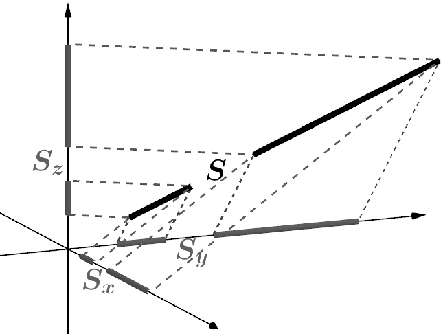
Figure 1: Real Pythagorean Theorem, $|S|^{2}_{1}=|S_{x}|^{2}_{1}+|S_{y}|^{2}_{1}+|S_{z}|^{2}_{1}$

Example 3.5.

Given $\mathds{C}$-orthogonal unit vectors $v_{1},v_{2}\in X$, and $c_{1},c_{2}\in\mathds{C}$ with $|c_{1}|^{2}+|c_{2}|^{2}=1$, let $v=c_{1}v_{1}+c_{2}v_{2}$. As pr:product projection factor gives $\pi_{\mathds{C}v,\mathds{C}v_{1}}=|c_{1}|^{2}$ and $\pi_{\mathds{C}v,\mathds{C}v_{2}}=|c_{2}|^{2}$, any area $A$ in $\mathds{C}v$ projects to $A_{1}=|c_{1}|^{2}\!\cdot\!A$ in $\mathds{C}v_{1}$ and to $A_{2}=|c_{2}|^{2}\!\cdot\!A$ in $\mathds{C}v_{2}$, with $A=A_{1}+A_{2}$ (fig:complexpythagorean).

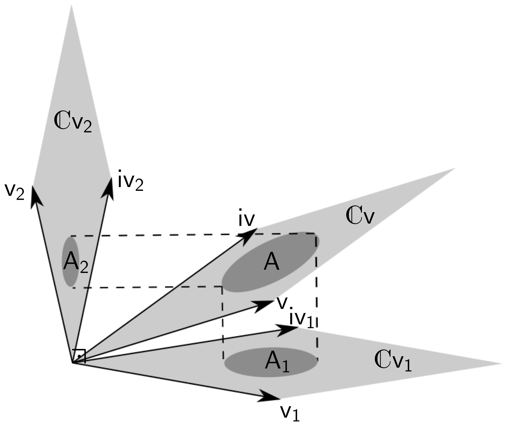
Figure 2: Complex Pythagorean Theorem, $A=A_{1}+A_{2}$

Similarities of this example with quantum theory are used in [Man19c] to obtain the Born rule in Everettian quantum mechanics.

Generalized Pythagorean theorems for subspaces other than lines involve projections on coordinate subspaces instead of a partition.

Let $\beta=(v_{1},\ldots,v_{n})$ be a basis of $X$, and $1\leq q\leq n$. For each multi-index $I=(i_{1},\ldots,i_{q})$, with $1\leq i_{1}<\ldots<i_{q}\leq n$, we write $V_{I}=\operatorname{span}(v_{i_{1}},\ldots,v_{i_{q}})$ and $\nu_{I}=v_{i_{1}}\wedge\ldots\wedge v_{i_{q}}\in\Lambda^{q}V_{I}$. The $\binom{n}{q}$ subspaces $V_{I}$ are the $q$-dimensional coordinate subspaces of $\beta$, and the $\nu_{I}$’s constitute a basis of $\Lambda^{q}X$, which is orthonormal if $\beta$ is orthonormal.

Proposition 3.6.

If $V\subset X$ is a subspace and $p=\dim V$ then

• $\sum_{I}\pi_{V,V_{I}}^{2}=1$ in the real case,

• $\sum_{I}\pi_{V,V_{I}}=1$ in the complex case,

where the sums run over all $p$-dimensional coordinate subspaces $V_{I}$ of an orthogonal basis of $X$.

Proof.

Without loss of generality, we can assume the basis is orthonormal. Let $\nu\in\Lambda^{p}V$ with $\|\nu\|=1$. Then $\sum_{I}|\langle\nu,\nu_{I}\rangle|^{2}=1$, and the result follows from pr:pi blades. ∎

This gives another Pythagorean theorem, relating the squared $p$-dimensional measure of a set in a real $p$-dimensional subspace to the squared measures of its projections on $p$-dimensional coordinate subspaces, and also a complex version with non-squared $2p$-dimensional measures.

Theorem 3.7 (Pythagorean theorem for subspaces).

Let $V\subset X$ be a subspace and $p=\dim V$. For any Lebesgue measurable set $S\subset V$,

• $|S|_{p}^{2}=\sum_{I}|S_{I}|_{p}^{2}$   in the real case,

• $|S|_{2p}=\sum_{I}|S_{I}|_{2p}$ in the complex case,

where the sums run over the orthogonal projections $S_{I}$ of $S$ on all $p$-dimensional coordinate subspaces of an orthogonal basis of $X$.

The real case gives, in particular, the following known generalizations of the Pythagorean theorem.

Example 3.8.

A tetrahedron $OABC$ is trirectangular at $O$ if all edges at this vertex are orthogonal to each other. De Gua’s Theorem (1783) [M.31] says the squared area of the face opposite such vertex equals the sum of the squared areas of the other faces (fig:tetraedro-edit). It extends to higher dimensional simplices [AMB96, Alv97, Cho91, DC35, LL90].

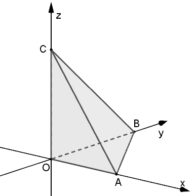
Figure 3: $\operatorname{area}(ABC)^{2}=\operatorname{area}(OAB)^{2}+\operatorname{area}(OAC)^{2}+\operatorname{area}(OBC)^{2}$

Example 3.9.

Since the XVIII century, it is known that the square of a planar area is the sum of the squares of its orthogonal projections on 3 mutually perpendicular planes [Eve90, p.450]. Conant and Beyer [CB74] have extended this to measurable sets (fig:projecao_snowflake) and any real dimension. They also tried to generalize it to the complex case, but the complex measure they used led to anomalous results. We note that much of their work can be replaced by rm:pi independent of S.

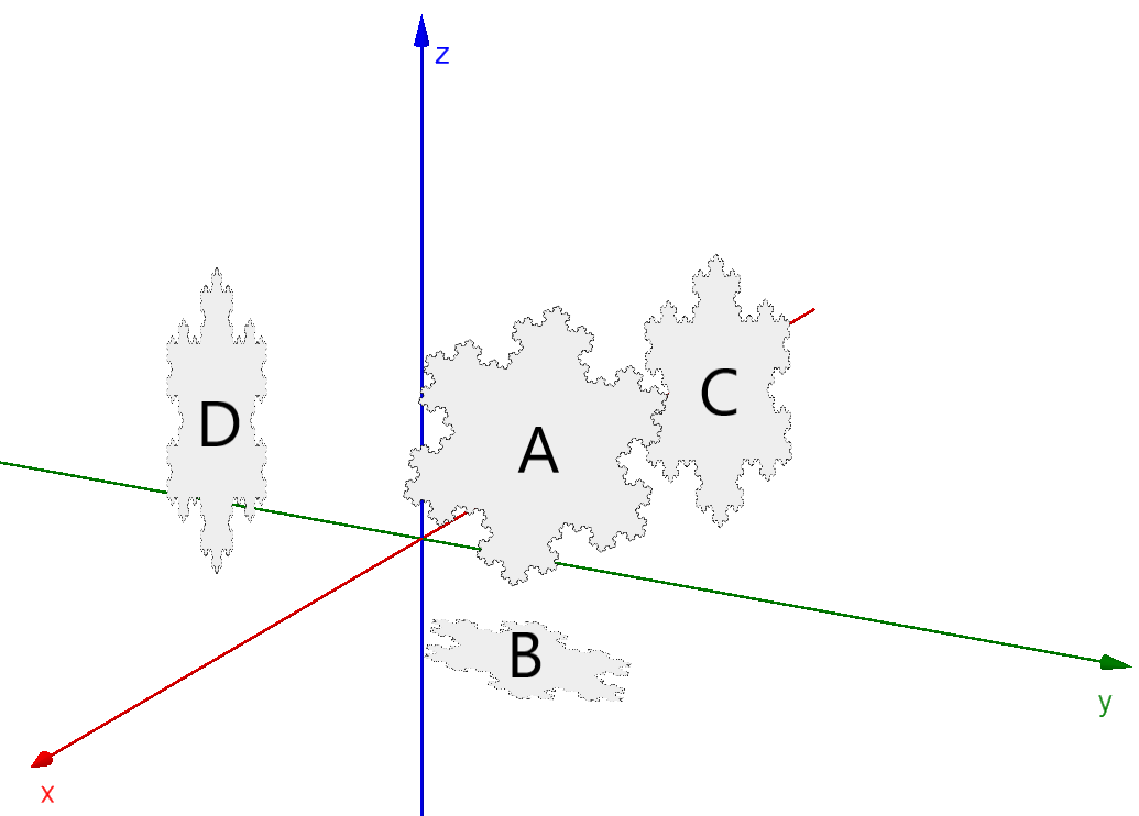
Figure 4: Projections of a Koch snowflake, $|A|_{2}^{2}=|B|_{2}^{2}+|C|_{2}^{2}+|D|_{2}^{2}$

Yet another Pythagorean theorem, for projections on coordinate subspaces of a different dimension than $V$, can be obtained using pr:projection Grassmann angle and identities for Grassmann angles proven in [Man19b].

Proposition 3.10.

Let $V\subset X$ be a subspace, $p=\dim V$, and $1\leq q\leq n=\dim X$. Then we have the following, where the sums run over all $q$-dimensional coordinate subspaces $V_{I}$ of an orthogonal basis of $X$.

1. If $p\leq q$ then

   • $\sum_{I}\pi_{V,V_{I}}^{2}=\binom{n-p}{n-q}$ in the real case,

   • $\sum_{I}\pi_{V,V_{I}}=\binom{n-p}{n-q}$ in the complex case.

2. If $p>q$ then

   • $\sum_{I}\pi_{V_{I},V}^{2}=\binom{p}{q}$ in the real case,

   • $\sum_{I}\pi_{V_{I},V}=\binom{p}{q}$ in the complex case.

Only the case $p\leq q$ gives a Pythagorean theorem.

Theorem 3.11.

Let $V\subset X$ be a subspace, $S\subset V$ be a Lebesgue measurable set, and $\dim V=p\leq q\leq n=\dim X$. Then

• $|S|_{p}^{2}=\binom{n-p}{n-q}^{-1}\cdot\sum_{I}|S_{I}|_{p}^{2}$   in the real case,

• $|S|_{2p}=\binom{n-p}{n-q}^{-1}\cdot\sum_{I}|S_{I}|_{2p}$ in the complex case,

where the sums run over the orthogonal projections $S_{I}$ of $S$ on all $q$-dimensional coordinate subspaces of an orthogonal basis of $X$.

The real case corresponds, when $S$ is a parallelotope, to a result of [Dru15]. The binomial coefficients appear because each projection on a $q$-dimensional coordinate subspace can be further decomposed into the $p$-dimensional coordinate subspaces it contains. And each of these belongs to $\binom{n-p}{q-p}=\binom{n-p}{n-q}$ of the $q$-dimensional ones.

Example 3.12.

Given a line segment of length $L$ in $\mathds{R}^{3}$, let $L_{xy},L_{xz}$ and $L_{yz}$ be the lengths of its orthogonal projections on the coordinate planes (fig:line_planes). Then $L^{2}=(L_{xy}^{2}+L_{xz}^{2}+L_{yz}^{2})/2$.

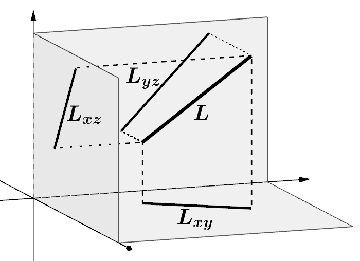
Figure 5: $L^{2}=(L_{xy}^{2}+L_{xz}^{2}+L_{yz}^{2})/2$

Using th:Pythagorean lines to relate $L$, $L_{xy}$, $L_{xz}$ and $L_{yz}$ to the orthogonal projections of these segments on the coordinate axes, one can easily see the reason for the factor $\frac{1}{2}$ in this example.

4 Final remarks

For simplicity, we have worked with linear subspaces of a finite dimensional inner product space $X$, but our results obviously extend to affine subspaces, and $X$ can be an infinite dimensional Hilbert space (however, $V$ must be finite dimensional and $W$ must be closed for $\pi_{V,W}$ to be defined).

That measures are not squared in the complex Pythagorean theorems is unusual, but the reason is clearly that each complex dimension corresponds to 2 real ones, both contracting by the same factor.

The same dimensional consideration suggests quaternionic versions should involve square roots of measures. Indeed, the tools used to get to th:Pythagorean lines also work in a complete quaternionic inner product space [Ist87, Rod14]. And essentially the same arguments can be used to show that, in such space, the square root of the 4-dimensional Lebesgue measure of a measurable set in a quaternionic line is the sum of the square roots of the measures of its orthogonal projections on the subspaces of an orthogonal partition. It would be interesting to know whether th:Pythagorean subspaces can also be extended to the quaternionic case.

The following examples show the complex case is actually simpler when calculations are carried out: there are less coordinate subspaces, and the measures add up in a simpler way. The real case leads to a messier calculation, in which it is almost surprising that the terms that appear when we expand the squares of the $|S_{ij}|_{2}$’s can be recombined into just the square of $|S|_{2}$.

Example 4.1.

In $\mathds{R}^{4}$, let $v=(a,b,c,d)\neq 0$, $u=(-b,a,-d,c)$ and $V=\operatorname{span}(v,u)$. If $\{v_{1},v_{2},v_{3},v_{4}\}$ is the canonical basis of $\mathds{R}^{4}$, let $P_{ij}$ be the orthogonal projection onto the coordinate subspace $V_{ij}=\operatorname{span}(v_{i},v_{j})$. The projections $S_{ij}$ of the square $S=[v,u]$ on the $V_{ij}$’s have measures $|S_{ij}|_{2}=\|P_{ij}v\wedge P_{ij}u\|$ given by

$$|S_{12}|_{2} =a^{2}+b^{2}, |S_{13}|_{2}=|S_{24}|_{2} =|bc-ad|,$$

$$|S_{34}|_{2} =c^{2}+d^{2}, |S_{14}|_{2}=|S_{23}|_{2} =|ac+bd|.$$

A calculation shows the sum of the squares of these six measures is equal to $(a^{2}+b^{2}+c^{2}+d^{2})^{2}=|S|_{2}^{2}$, in accordance with th:Pythagorean subspaces.

Example 4.2.

The previous example can be reframed in complex terms. Identifying $\mathds{C}^{2}$ with $\mathds{R}^{4}$ we have $v=(a+ib,c+id)$, $u=iv$ and $V=\mathds{C}v$. Of the $V_{ij}$’s, only $V_{12}$ and $V_{34}$ are complex subspaces (invariant under multiplication by $\mathrm{i}$), corresponding to the complex coordinate lines of the canonical basis $\{(1,0),(0,1)\}$ of $\mathds{C}^{2}$. One can immediately see that, in accordance with th:Pythagorean lines, $|S_{12}|_{2}+|S_{34}|_{2}=a^{2}+b^{2}+c^{2}+d^{2}=|S|_{2}$.

The many properties projection factors have (including those in the appendix), and the ease with which the generalized Pythagorean theorems were obtained using them, suggest they should have other applications.

As noted, they have unexpected connections with quantum theory. In [Man19c] we show the complex case of th:Pythagorean lines can be used, with some extra physical assumptions, to obtain the Born rule and solve the probability problem of Everettian quantum mechanics, with projection factors actually playing the role of quantum probabilities.

Appendix A Properties of projection factors

Many properties of projection factors are listed below. Some can be easily obtained from the definition and results presented in this article, while others follow from pr:projection Grassmann angle and properties of Grassmann angles proven in [Man19a, Man19b].

Proposition A.1.

Let $V,W\subset X$ be nonzero subspaces, $p=\dim V$, $q=\dim W$, and $P:V\rightarrow W$ be the orthogonal projection.

1. $\pi_{\{0\},\{0\}}=\pi_{\{0\},W}=1$ and $\pi_{V,\{0\}}=0$.

2. $\pi_{V,W}=0\ \Leftrightarrow\ V\cap W^{\perp}\neq\{0\}$.

3. $\pi_{V,W}=1\ \Leftrightarrow\ V\subset W$.

4. $\pi_{V,W}=\pi_{V,P(V)}$.

5. If $\dim V=\dim W$ then $\pi_{V,W}=\pi_{W,V}$.

6. In the complex case (with $W$ complex), for any $v\in X$ and any nonzero $u\in\mathds{C}v$ we have $\pi_{\mathds{C}v,W}=\pi^{2}_{\mathds{R}v,W}$ and $\pi_{\mathds{R}u,W}=\pi_{\mathds{R}v,W}$.

7. If $V^{\prime}$ and $W^{\prime}$ are the orthogonal complements of $V\cap W$ in $V$ and $W$, respectively, then $\pi_{V,W}=\pi_{V^{\prime},W^{\prime}}$.

8. If $V=\bigoplus_{i}V_{i}$, with the $V_{i}$’s being mutually orthogonal subspaces spanned by principal vectors of $V$ w.r.t. $W$, then $\pi_{V,W}=\prod_{i}\pi_{V_{i},W}$.

9. If $V=A\oplus B$, with $A\perp B$, then

   $$\pi_{V,W}=\pi_{A,W}\cdot\pi_{B,W}\cdot\pi_{P(A),P(B)^{\perp}}.$$

10. For any subspace $U\subset W$, $\pi_{V,U}=\pi_{V,W}\cdot\pi_{P(V),U}$.

11. $\pi_{V,W}\leq\pi_{m}$, where $\pi_{m}$ is the smallest principal projection factor of $V$ and $W$.

12. $\pi_{V,W^{\prime}}\leq\pi_{V,W}$ for any subspace $W^{\prime}\subset W$, with equality if, and only if, $V\cap W^{\perp}\neq\{0\}$ or $P(V)\subset W^{\prime}$.

13. $\pi_{V^{\prime},W}\geq\pi_{V,W}$ for any subspace $V^{\prime}\subset V$, with equality if, and only if, $V^{\prime}\cap W^{\perp}\neq\{0\}$ or $V\cap V^{\prime\perp}\subset W$.

14. Let $\mathcal{P}\nu=Pv_{1}\wedge\ldots\wedge Pv_{p}$ be the orthogonal projection on $\Lambda^{p}W$ of a blade $\nu=v_{1}\wedge\ldots\wedge v_{p}\in\Lambda^{p}V$. Then

    • $\|\mathcal{P}\nu\|=\|\nu\|\cdot\pi_{V,W}$     in the real case,

    • $\|\mathcal{P}\nu\|^{2}=\|\nu\|^{2}\cdot\pi_{V,W}$   in the complex case.

15. Given nonzero blades $\nu\in\Lambda^{p}V$ and $\omega\in\Lambda^{q}W$,

    $$\pi_{V,W}=\begin{cases}\hskip 2.0pt\frac{\|\nu\lrcorner\,\omega\|}{\|\nu\|\|\omega\|}\ \ \,\text{ in the real case,}\\[5.0pt] \frac{\|\nu\lrcorner\,\omega\|^{2}}{\|\nu\|^{2}\|\omega\|^{2}}\ \text{ in the complex case,}\end{cases}$$

    where $\lrcorner\,$ is the interior product of blades [Man19b].

16. If $U\subset V$ is a subspace and $r=\dim U$,

    $$\pi_{U,W}=\begin{cases}\sqrt{\sum_{I}\pi^{2}_{U,V_{I}}\cdot\pi^{2}_{V_{I},W}}\ \ \,\text{ in the real case,}\\[5.0pt] \hskip 9.0pt\sum_{I}\pi_{U,V_{I}}\cdot\pi_{V_{I},W}\hskip 8.0pt\text{ in the complex case.}\end{cases}$$

    where the sums run over all $r$-dimensional coordinate subspaces $V_{I}$ of a principal basis of $V$ with respect to $W$.

There are also several properties for projection factors with the orthogonal complement of a subspace.

Proposition A.2.

Let $V,W\subset X$ be nonzero subspaces, $p=\dim V$, $q=\dim W$ and $m=\min\{p,q\}$.

1. $\pi_{V,W^{\perp}}=\pi_{W,V^{\perp}}$.

2. $\pi_{V^{\perp},W^{\perp}}=\pi_{W,V}$.

3. If $\pi_{1},\ldots,\pi_{m}$ are the principal projection factors of $V$ and $W$ then

   $$\pi_{V,W^{\perp}}=\begin{cases}\prod_{i=1}^{m}\sqrt{1-\pi_{i}^{2}}\,\text{ in the real case,}\\[5.0pt] \prod_{i=1}^{m}(1-\pi_{i})\ \ \text{ in the complex case.}\end{cases}$$

4. For $\zeta(V,W)=\begin{cases}\pi^{2}_{V,W}+\pi^{2}_{V,W^{\perp}}\ \text{(real case)}\\ \pi_{V,W}+\pi_{V,W^{\perp}}\text{ (complex case)}\end{cases}$ we have:

   • $0\leq\zeta(V,W)\leq 1$;

   • $\zeta(V,W)=1\ \Leftrightarrow\ \dim V=1$, or $V\subset W$, or $V\perp W$;

   • $\zeta(V,W)=0\ \Leftrightarrow\ V\cap W\neq\{0\}$ and $V\cap W^{\perp}\neq\{0\}$.

5. Given nonzero blades $\nu\in\Lambda^{p}V$ and $\omega\in\Lambda^{q}W$,

   $$\pi_{V,W^{\perp}}=\begin{cases}\hskip 2.0pt\frac{\|\nu\wedge\omega\|}{\|\nu\|\|\omega\|}\ \ \,\text{ in the real case,}\\[5.0pt] \frac{\|\nu\wedge\omega\|^{2}}{\|\nu\|^{2}\|\omega\|^{2}}\ \text{ in the complex case.}\end{cases}$$

6. Given any bases $(v_{1},\ldots,v_{p})$ of $V$ and $(w_{1},\ldots,w_{q})$ of $W$, let $A=\big{(}\langle w_{i},w_{j}\rangle\big{)}$, $B=\big{(}\langle w_{i},v_{j}\rangle\big{)}$, and $D=\big{(}\langle v_{i},v_{j}\rangle\big{)}$. Then

   $$\pi_{V,W^{\perp}}=\begin{cases}\sqrt{\frac{\det(A-BD^{-1}B^{T})}{\det A}}\ \,\text{ in the real case,}\\[5.0pt] \ \ \frac{\det(A-BD^{-1}\bar{B}^{T})}{\det A}\ \ \text{ in the complex case.}\end{cases}$$

   If both bases are orthonormal then

   $$\pi_{V,W^{\perp}}=\begin{cases}\sqrt{\det\left(\mathds{1}_{q\times q}-BB^{T}\right)}\ \,\text{ in the real case,}\\ \ \ \det\left(\mathds{1}_{q\times q}-B\bar{B}^{T}\right)\ \,\text{ in the complex case.}\end{cases}$$

References

- [Alv97] S.A. Alvarez, Note on an n-dimensional Pythagorean theorem, \urlhttp://www.cs.bc.edu/ alvarez/NDPyt.pdf, 1997, Accessed: 2019-10-25.
- [AMB96] A.R. Amir-Moéz and R.E. Byerly, Pythagorean theorem in unitary spaces, Univ. Beograd, Publ. Elektrotehn. Fak., Ser. Mat. (1996), no. 7, 85–89.
- [Atz00] E.J. Atzema, Beyond Monge’s theorem: A generalization of the Pythagorean theorem, Math. Mag. 73 (2000), no. 4, 293–296.
- [BŻ17] I. Bengtsson and K. Życzkowski, Geometry of quantum states: an introduction to quantum entanglement, Cambridge University Press, 2017.
- [CB74] D.R. Conant and W.A. Beyer, Generalized Pythagorean theorem, Amer. Math. Monthly 81 (1974), no. 3, 262–265.
- [Cho91] E.C. Cho, The generalized cross product and the volume of a simplex, Appl. Math. Lett. 4 (1991), no. 6, 51–53.
- [DC35] P S. Donchian and H. S. M. Coxeter, An n-dimensional extension of Pythagoras’ theorem, Math. Gaz. 19 (1935), no. 234, 206–206.
- [Dix49] J. Dixmier, Étude sur les variétés et les opérateurs de Julia, avec quelques applications, Bull. Soc. Math. France 77 (1949), 11–101.
- [Dru15] D. Drucker, A comprehensive Pythagorean theorem for all dimensions, Amer. Math. Monthly 122 (2015), no. 2, 164–168.
- [EI57] H. Everett III, Relative state formulation of quantum mechanics, Rev. Mod. Phys. 29 (1957), no. 3, 454–462.
- [ER08] L. Eifler and N.H. Rhee, The n-dimensional Pythagorean theorem via the divergence theorem, Amer. Math. Monthly 115 (2008), no. 5, 456–457.
- [Eve90] H.W. Eves, An introduction to the history of mathematics, 6 ed., Saunders Series, Holt, Rinehart and Winston, 1990.
- [Fri37] K. Friedrichs, On certain inequalities and characteristic value problems for analytic functions and for functions of two variables, Trans. Amer. Math. Soc. 41 (1937), no. 3, 321–364.
- [Gan00] F.R. Gantmacher, The theory of matrices, AMS Chelsea Publishing Series, vol. 1, Chelsea Publishing Company, 2000.
- [GH06] A. Galántai and C.J. Hegedűs, Jordan’s principal angles in complex vector spaces, Numer. Linear Algebra Appl. 13 (2006), no. 7, 589–598.
- [Glu67] H. Gluck, Higher curvatures of curves in Euclidean space, II, Amer. Math. Monthly 74 (1967), no. 9, 1049–1056.
- [GNSB05] H. Gunawan, O. Neswan, and W. Setya-Budhi, A formula for angles between subspaces of inner product spaces, Beitr. Algebra Geom. 46 (2005), no. 2, 311–320.
- [Hit10] E. Hitzer, Angles between subspaces computed in Clifford algebra, AIP Conference Proceedings, vol. 1281, AIP, 2010, pp. 1476–1479.
- [Ist87] V. Istratescu, Inner product structures: Theory and applications, Springer Netherlands, 1987.
- [Jia96] S. Jiang, Angles between Euclidean subspaces, Geom. Dedicata 63 (1996), 113–121.
- [LL90] S.Y. Lin and Y.F. Lin, The n-dimensional Pythagorean theorem, Linear Multilinear Algebra 26 (1990), no. 1-2, 9–13.
- [M.31] F. G. M., Exercices de géométrie: comprenant l’exposé des méthodes géométriques et 2000 questions résolues, Cours de mathématiques élémentaires, Librairie Générale, 1931.
- [Man19a] A.L.G. Mandolesi, Grassmann angles between real or complex subspaces, arXiv:math.GM/1910.00147 (2019).
- [Man19b] , Products of simple multivectors and Grassmann angle identities, arXiv:math.GM/1910.07327 (2019).
- [Man19c] , Quantum fractionalism: the Born rule as a consequence of the complex Pythagorean theorem, arXiv:quant-ph/1905.08429 (2019).
- [Rod14] L. Rodman, Topics in quaternion linear algebra, Princeton University Press, 2014.
- [Rud86] W. Rudin, Real and complex analysis, 3 ed., McGraw-Hill, 1986.
- [SBKW10] S. Saunders, J. Barrett, A. Kent, and D. Wallace (eds.), Many worlds? Everett, quantum theory & reality, Oxford University Press, 2010.
- [Sch01] K. Scharnhorst, Angles in complex vector spaces, Acta Appl. Math. 69 (2001), no. 1, 95–103.
- [SKM89] P.K. Suetin, A.I. Kostrikin, and Y.I. Manin, Linear algebra and geometry, CRC Press, 1989.
- [Wed83] P. Wedin, On angles between subspaces of a finite dimensional inner product space, Matrix Pencils, Lecture Notes in Mathematics, vol. 973, Springer, 1983, pp. 263–285.
- [Win10] S. Winitzki, Linear algebra via exterior products, Ludwig-Maximilians University, Munich, Germany, 2010.
- [Won67] Y. Wong, Differential geometry of Grassmann manifolds, Proc. Natl. Acad. Sci. USA 57 (1967), no. 3, 589–594.
- [Yok92] T. Yokonuma, Tensor spaces and exterior algebra, Translations of Mathematical Monographs, American Mathematical Society, 1992.