On the number of intersection points of the contour of an amoeba with a line

Abstract.

In this note, we investigate the maximal number of intersection points of a line with the contour of hypersurface amoebas in $\mathbb{R}^{n}$. We define the latter number to be the $\mathbb{R}$-degree of the contour. We also investigate the $\mathbb{R}$-degree of related sets such as the boundary of amoebas and the amoeba of the real part of hypersurfaces defined over $\mathbb{R}$. For all these objects, we provide bounds for the respective $\mathbb{R}$-degrees.

1. Introduction

Amoebas of algebraic hypersurfaces in $(\mathbb{C}^{\star})^{n}$ were introduced in 1994 in [GKZ] and since then have been one of the central objects of study in tropical geometry. (An accessible introduction to amoebas can be found in [Vi02].) Amoebas enjoy a number of beautiful and important properties such as special asymptotics at infinity and convexity of all connected components of the complement, to mention a few. One way to understand the geometry of amoebas goes by studying its contour. In this perspective, we introduce the following.

Definition 1.

Given a closed semi-analytic hypersurface $H\subset\mathbb{R}^{n}$ without boundary, we define the $\mathbb{R}$-degree $\mathbb{R}\deg(H)$ as the supremum of the cardinality of $H\cap L$ taken over all lines $L\subset\mathbb{R}^{n}$ such that $L$ intersects $H$ transversally. (Observe that we count points in $H\cap L$ without multiplicity)

Our aim in this note is to provide estimates for the $\mathbb{R}$-degree of four closely related types of sets $H$, namely when $H$ is

– a tropical hypersurface,

– the boundary of the amoeba of a hypersurface $\mathcal{H}\subset(\mathbb{C}^{\star})^{n}$,

– the amoeba of the real locus of a hypersurface $\mathcal{H}\subset(\mathbb{C}^{\star})^{n}$ defined over $\mathbb{R}$,

– the contour of the amoeba of a hypersurface $\mathcal{H}\subset(\mathbb{C}^{\star})^{n}$.
In particular, we will show that $\mathbb{R}\deg(H)$ is always finite for all $H$ as above.

For a subset $H\subset\mathbb{R}^{n}$ that is real-algebraic (respectively piecewise real-algebraic), the $\mathbb{R}$-degree satisfies $\mathbb{R}\deg(H)\leqslant\deg(H)$, where $\deg(H)$ is the usual degree of $H$ (respectively the sum of the degrees of the algebraic continuation of each piece of $H$). In particular, the $\mathbb{R}$-degree of a real-algebraic hypersurface is always finite. More generally, if $H$ is piecewise real-analytic, then it can happen that either $\mathbb{R}\deg(H)=\infty$ or $\mathbb{R}\deg(H)<\infty$ although the degree of the analytic continuation of $H$, is always infinite.

We begin our investigation of the $\mathbb{R}$-degree with the case of tropical hypersurfaces. Recall that for a finite set $\mathcal{M}\subset\mathbb{Z}^{n}$, a tropical polynomial supported on $\mathcal{M}$ is a convex piecewise linear function $p:\mathbb{R}^{n}\rightarrow\mathbb{R}^{n}$ of the form

$$p(x)=\max_{\alpha\in\mathcal{M}}\left\langle\,x\,|\,\alpha\,\right\rangle+c_{\alpha}$$

where $c_{\alpha}\in\mathbb{R}$. The tropical hypersurface associated to $p$ is the set of points $x\in\mathbb{R}^{n}$ for which $f(x)$ is equal to at least two of its tropical monomials $\left\langle\,x\,|\,\alpha\,\right\rangle+c_{\alpha}$. We refer to [IMS] for the basic notions. We have the following estimate.

Proposition 1.

Let $\mathcal{M}\subset\mathbb{Z}^{n}$ be any finite set. For any tropical hypersurface $H\subset\mathbb{R}^{n}$ defined by a tropical polynomial supported on $\mathcal{M}$, one has

$$\mathbb{R}\deg(H)\leqslant\#\mathcal{M}-1.$$

Moreover, there always exists a tropical hypersurface $H$ supported on $\mathcal{M}$ such that $\mathbb{R}\deg(H)=\#\mathcal{M}-1.$

For a finite set $\mathcal{M}\subset\mathbb{Z}^{n}$ of Laurent monomials, denote by $|\mathcal{L}_{\mathcal{M}}|$ the space of all Laurent polynomials supported on $\mathcal{M}$, up to projective equivalence. For a hypersurface $\mathcal{H}\subset(\mathbb{C}^{\star})^{n}$ given by $\{P=0\}$ where $P\in|\mathcal{L}_{\mathcal{M}}|$, denote by $\mathcal{A}_{\mathcal{H}}\subset\mathbb{R}^{n}$ its amoeba, i.e. the image of $\mathcal{H}$ under the logarithmic map

$$\begin{array}[]{rcl}\text{Log}\quad:\quad(\mathbb{C}^{\star})^{n}&\to&\mathbb{R}^{n}\\ (z_{1},\dots,z_{n})&\mapsto&(\log|z_{1}|,\dots,\log|z_{n}|)\end{array}.$$

Denote by $\partial\mathcal{A}_{\mathcal{H}}\subset\mathcal{A}_{\mathcal{H}}$ the boundary of $\mathcal{A}_{\mathcal{H}}$ and define the critical locus $\mathfrak{C}_{\mathcal{H}}\subset\mathcal{H}$ to be the set of critical points of the restriction of the map Log to $\mathcal{H}$. The contour $\mathcal{C}\mathcal{A}_{\mathcal{H}}\subset\mathcal{A}_{\mathcal{H}}$ is the set of critical values of $\text{Log}_{|\mathcal{H}}$, i.e. $\mathcal{C}\mathcal{A}_{\mathcal{H}}=\text{Log}(\mathfrak{C}_{\mathcal{H}})$. Finally, denote by $\mathcal{S}\mathcal{A}_{\mathcal{H}}$ the spine of $\mathcal{A}_{\mathcal{H}}$, see [PR]. We refer to Figures 1 and 3 and [BKS] for further illustrations. More details about the spine and the contour of amoebas can be found in [PT08].

It is known that the critical locus $\mathfrak{C}_{\mathcal{H}}$ is a real-algebraic subvariety in $(\mathbb{C}^{\star})^{n}$. The latter follows from the description of $\mathfrak{C}_{\mathcal{H}}\subset\mathcal{H}$ as the pullback of $\mathbb{R}P^{n-1}$ under the logarithmic Gauss map $\gamma_{\mathcal{H}}:\mathcal{H}\to\mathbb{C}P^{n-1}$ given by

$$\gamma_{\mathcal{H}}(z_{1},\dots,z_{n})=\big{[}z_{1}\cdot\partial_{z_{1}}P;\dots;z_{n}\cdot\partial_{z_{n}}P\big{]}$$

where $P$ is a defining polynomial of $\mathcal{H}$, see [Mi00, Lemma 3]. Since $\mathcal{C}\mathcal{A}_{\mathcal{H}}$ is the image of $\mathfrak{C}_{\mathcal{H}}$ under the analytic map Log, the contour $\mathcal{C}\mathcal{A}_{\mathcal{H}}$ is necessarily semi-analytic, that is $\mathcal{C}\mathcal{A}_{\mathcal{H}}$ is defined by analytic equations and inequalities. It is claimed at various places in the literature that $\mathcal{C}\mathcal{A}_{\mathcal{H}}$ is actually analytic. The latter fact is not true in general as illustrated by Example 2 in [Mi00], see Section 2 for further details. Instead, we have the following.

Lemma 1.

For any algebraic hypersurface $\mathcal{H}\subset(\mathbb{C}^{\star})^{n}$, the contour $\mathcal{C}\mathcal{A}_{\mathcal{H}}$ and the boundary $\partial\mathcal{A}_{\mathcal{H}}$ are closed semi-analytic hypersurfaces without boundary in $\mathbb{R}^{n}$.

Let us also mention that the contour $\mathcal{C}\mathcal{A}_{\mathcal{H}}$ may have components of various dimensions. Although such phenomenon has not been observed by the authors, this occurs for the critical locus of the coordinatewise argument map $\operatorname{Arg}$ (consider real hypersurfaces for instance). Since, in logarithmic coordinates, Log and $\operatorname{Arg}$ are the projection onto the real and imaginary axes respectively, there is a priori no reason why the latter phenomenon should appear only on one side of the picture.

Let us now discuss the $\mathbb{R}$-degree of the boundary of hypersurface amoebas. In that perspective, observe that the spine $\mathcal{S}\mathcal{A}_{\mathcal{H}}\subset\mathbb{R}^{n}$ is a tropical hypersurface (see [PT08]).

Proposition 2.

Let $\mathcal{M}\subset\mathbb{Z}^{n}$ be a finite set of Laurent monomials. For any hypersurface $\mathcal{H}\subset(\mathbb{C}^{\star})^{n}$ given by $\{P=0\}$ where $P\in|\mathcal{L}_{\mathcal{M}}|$, one has

$$\mathbb{R}\deg(\partial\mathcal{A}_{\mathcal{H}})\leqslant 2\cdot\mathbb{R}\deg(\mathcal{S}\mathcal{A}_{\mathcal{H}}).$$

Moreover, there always exists $P\in|\mathcal{L}_{\mathcal{M}}|$ such that $\mathbb{R}\deg(\partial\mathcal{A}_{\mathcal{H}})=2\cdot\mathbb{R}\deg(\mathcal{S}\mathcal{A}_{\mathcal{H}})$.

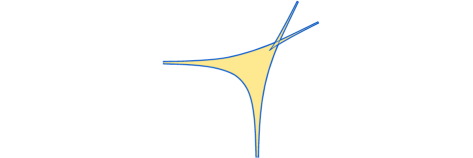
Figure 1. Amoeba of the discriminant $27+4a^{3}-18ab-a^{2}b^{2}+4b^{3}$ of the family $1+ax+bx^{2}+x^{3}$ and its contour (in blue).

Observe that for a particular $P\in|\mathcal{L}_{\mathcal{M}}|$, the inequality in Proposition 2 can be strict, see e.g. Figure 2. Since the support of a tropical polynomial defining the spine $\mathcal{S}\mathcal{A}_{\mathcal{H}}$ can be always taken as a subset of $\Delta\cap\mathbb{Z}^{n}$ where $\Delta$ is the convex hull of $\mathcal{M}$ in $\mathbb{R}^{n}=\mathbb{Z}^{n}\otimes_{\mathbb{Z}}\mathbb{R}$, the following statement is a consequence of Propositions 1 and 2.

Corollary 1.

Under the assumptions of Proposition 2, one has

$$\mathbb{R}\deg(\partial\mathcal{A}_{\mathcal{H}})\leqslant 2\big{(}\#(\Delta\cap\mathbb{Z}^{n})-1\big{)}$$

where $\Delta$ is the convex hull of $\mathcal{M}$.

Proposition 3.

Let $\mathcal{M}\subset\mathbb{Z}^{n}$ be a finite set of Laurent monomials and denote $\Delta:=\operatorname{conv}(\mathcal{M})$. For any contractible tropical hypersurface $T\subset\mathbb{R}^{n}$ supported on $\mathcal{M}$, one has

$$\mathbb{R}\deg(T)\leqslant\#\widetilde{\mathcal{M}}-1$$

where $\widetilde{\mathcal{M}}:=\mathcal{M}\cap\partial\Delta$. For a hypersurface $\mathcal{H}\in|\mathcal{L}_{\mathcal{M}}|$ with contractible amoeba, one has

$$\mathbb{R}\deg(\partial\mathcal{A}_{\mathcal{H}})\leqslant 2\big{(}\#(\partial\Delta\cap\mathbb{Z}^{n})-1\big{)}.$$

In the case of curves, we can prove a stronger statement than Corollary 1. Recall that for a non-degenerate lattice polygon $\Delta\subset\mathbb{R}^{2}$, i.e. $\operatorname{int}(\Delta)\neq\emptyset$, we can construct a toric surface $X_{\Delta}$ together with the tautological linear system $|\mathcal{L}_{\Delta}|$. Denote by $V_{\Delta,g}\subset|\mathcal{L}_{\Delta}|$ the Severi variety parametrizing irreducible curves of genus $g$, where $0\leqslant g\leqslant\#(\operatorname{int}(\Delta)\cap\mathbb{Z}^{2})$.

Proposition 4.

Let $\Delta\subset\mathbb{R}^{2}$ be a non-degenerate lattice polygon. Then, for any $0\leqslant g\leqslant\#(\textrm{int}(\Delta)\cap\mathbb{Z}^{2})$ and any curve $\mathcal{H}\in V_{\Delta,g}$, one has

$$\mathbb{R}\deg(\partial\mathcal{A}_{\mathcal{H}})\leqslant 2(\#(\partial\Delta\cap\mathbb{Z}^{2})-1+g).$$

Furthermore, this upper bound is sharp.

Let us now consider the situation when $\mathcal{H}\subset(\mathbb{C}^{\star})^{n}$ is a real hypersurface, i.e. its defining polynomial $P$ can be chosen to have real coefficients. Denote by $\mathcal{H}_{\mathbb{R}}:=\mathcal{H}\cap(\mathbb{R}^{\ast})^{n}$ the set of real point of $\mathcal{H}$ and define the real stratum of the amoeba $\mathcal{A}_{\mathcal{H}}$ to be the set $\mathcal{A}_{\mathcal{H}}^{\mathbb{R}}:=\text{Log}(\mathcal{H}_{\mathbb{R}})$. As a consequence of [Mi00, Lemma 3], one has the inclusions $\mathcal{H}_{\mathbb{R}}\subset\mathfrak{C}_{\mathcal{H}}$ and $\mathcal{A}_{\mathcal{H}}^{\mathbb{R}}\subset\mathcal{C}\mathcal{A}_{\mathcal{H}}$.

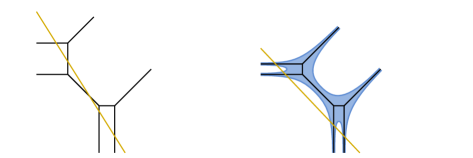
Figure 2. A tropical conic (left) and the amoeba of a conic (right) together with lines realizing their $\mathbb{R}$-degrees. On the right, the bounds given by Propositions 2 and 4 coincide and neither of them is sharp.

Our next goal is to estimate the $\mathbb{R}$-degree of $\mathcal{A}_{\mathcal{H}}^{\mathbb{R}}$ in terms of the support $\mathcal{M}$ of $\mathcal{H}\subset(\mathbb{C}^{\star})^{n}$. To formulate the answer, we need to consider the action of the group $\{\pm 1\}^{n}$ of the sign changes of coordinates $(z_{1},z_{2},\dots,z_{n})$ on the space $\{\pm 1\}^{\mathcal{M}}$ of all possible sign patterns of the monomials in $\mathcal{M}$. A sign change of coordinates $\varepsilon=(\varepsilon_{1},\cdots,\varepsilon_{n})\in\{\pm 1\}^{n}$ acts on a sign pattern $\sigma=(\sigma_{\alpha})_{\alpha\in\mathcal{M}}$ by $\varepsilon\cdot\sigma=(\sigma_{\alpha}\varepsilon^{\alpha})_{\alpha\in\mathcal{M}}$ where $\varepsilon^{\alpha}=\varepsilon_{1}^{\alpha_{1}}\cdots\varepsilon_{n}^{\alpha_{n}}$ and $\alpha=(\alpha_{1},\cdots,\alpha_{n})$. Clearly, the cardinality of the orbit $\{\pm 1\}^{n}\cdot\sigma$ is a power of $2$ and depends only on $\mathcal{M}$. It is therefore denoted by $2^{\kappa_{\mathcal{M}}}$. Notice also that either $\{\pm 1\}^{n}\cdot\sigma=-\{\pm 1\}^{n}\cdot\sigma$, or $\big{(}\{\pm 1\}^{n}\cdot\sigma\big{)}\cap\big{(}-\{\pm 1\}^{n}\cdot\sigma\big{)}=\emptyset$ and that $\{\pm 1\}^{n}\cdot\sigma=-\{\pm 1\}^{n}\cdot\sigma$ for some $\sigma\in\{\pm 1\}^{\mathcal{M}}$ if and only if it holds for all $\sigma\in\{\pm 1\}^{\mathcal{M}}$.

Proposition 5.

Let $\mathcal{M}\subset\mathbb{Z}^{n}$ be a finite set of Laurent monomials. For any hypersurface $\mathcal{H}\subset(\mathbb{C}^{\star})^{n}$ given by $\{P=0\}$ where $P\in|\mathcal{L}_{\mathcal{M}}|$ is a real polynomial, one has

• if $\{\pm 1\}^{n}\cdot\sigma=-\{\pm 1\}^{n}\cdot\sigma$ for all $\sigma\in\{\pm 1\}^{\mathcal{M}}$, then

  $$\mathbb{R}\deg(\mathcal{A}_{\mathcal{H}}^{\mathbb{R}})\leqslant\begin{cases}\#\mathcal{M}-1,\quad&\text{for}\ \kappa_{\mathcal{M}}=1,\\ 2^{\kappa_{\mathcal{M}}-1}(2\#\mathcal{M}-3),\quad&\text{for}\ \kappa_{\mathcal{M}}\geqslant 2,\end{cases}$$

• if $\big{(}\{\pm 1\}^{n}\cdot\sigma\big{)}\cap\big{(}-\{\pm 1\}^{n}\cdot\sigma\big{)}=\emptyset$ for all $\sigma\in\{\pm 1\}^{\mathcal{M}}$, then

  $$\mathbb{R}\deg(\mathcal{A}_{\mathcal{H}}^{\mathbb{R}})\leqslant\begin{cases}\#\mathcal{M}-1,\quad&\text{for}\ \kappa_{\mathcal{M}}=0,\\ 2^{\kappa_{\mathcal{M}}-1}(2\#\mathcal{M}-3),\quad&\text{for}\ \kappa_{\mathcal{M}}\geqslant 1.\end{cases}$$

Finally, we consider the contour of a hypersurface in $(\mathbb{C}^{\star})^{n}$. Using Khovanskii’s fewnomial theory, we obtain the following upper bound for the $\mathbb{R}$-degree of the contour.

Proposition 6.

For any hypersurface $\mathcal{H}\subset(\mathbb{C}^{\star})^{n}$ defined by a polynomial $P$ of degree $d$, one has

$$\mathbb{R}\deg(\mathcal{C}\mathcal{A}_{\mathcal{H}})\leqslant 2^{2n+(n-1)(n-2)/2}d^{n+1}\Big{(}4dn+2(n-1)^{2}-1\Big{)}^{n-1}.$$

The upper bound of the above proposition is probably not sharp, as illustrated by the following improvement in dimension $2$ in which case we take into account the combinatorics of the Newton polygon of the curve.

Proposition 7.

For any curve $\mathcal{H}\subset(\mathbb{C}^{\star})^{2}$ defined by a bivariate polynomial $P$ of degree $d$ and with Newton polygon $\Delta$, one has

$$\mathbb{R}\deg(\mathcal{C}\mathcal{A}_{\mathcal{H}})\leqslant 4d^{3}(4d-2)+\#(\partial\Delta\cap\mathbb{Z}^{2})-\text{Area}(\Delta)$$

where $\text{Area}(\Delta)$ is twice the Euclidean area of $\Delta$.

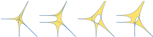
Figure 3. Amoebas of curves with Newton polygon $\operatorname{conv}\{(0,0),(1,0),(2,1),(0,2)\}$ with their respective contour (in blue).

While proving Proposition 7, we additionally provide an upper bound on the number of cusps of the contour $\mathcal{C}\mathcal{A}_{\mathcal{H}}$, see Corollary 2. The latter quantity is intimately related to the analogue of Hilbert’s sixteenth problem for amoebas considered in [La].

To conclude the introduction, let us mention that the subject of this paper is a particular instance of the general problem of finding estimates for the number of real solutions to systems of (semi)-analytic equations. The most well-known example is the fewnomial theory developed by A. Khovanskii in [Kh] where the considered systems of equations are given by (semi)-Pfaffian functions.

Being the image of the (real algebraic) critical locus of a complex hypersurface under the logarithmic map, the contour of an amoeba is the zero set of a sub-Pfaffian function. (Amoebas’ boundary is also defined by a sub-Pfaffian function).

We think that the existing methods of obtaining upper bounds in the fewnomial theory, mainly based on the so-called Rolle-Khovanskii lemma are not very effective for amoebas. Indeed, most of the equations of the Pfaffian system defining the critical locus $\mathfrak{C}_{\mathcal{H}}$ depend only the single polynomial equation $P$ defining the hypersurface $\mathcal{H}\subset(\mathbb{C}^{\star})^{n}$. In particular, the latter system is highly non-generic. The upper bound from Proposition 7 comes from convexity of the components of the complement to an amoeba and other topological considerations which are different type of phenomena as compared to the Rolle-Khovanskii type of observations.

The structure of the paper is as follows. Section 2 contains the proofs of the above statements and Section 3 contains some discussions and further outlook.

Acknowledgements. The first and the third authors want to thank the Mittag-Leffler institute for the hospitality in Spring 2018. The second author wants to acknowledge the financial support of his research provided by the Swedish Research Council grant 2016-04416. The second author is sincerely grateful to D. Novikov and T. Sadykov for discussions and their interest in this project. The authors thank D. Bogdanov for providing an online tool for automated generation of MATLAB code available for free public use at http://dvbogdanov.ru/?page=amoeba and his help with creating Fig. 3.

2. Proofs

We begin this section with a general remark that we will use repeatedly.

Remark 1.

For any continuous family of lines $L_{t}$ intersecting $H$ transversally, the number of points $\#(L_{t}\cap H)$ is a lower semi-continuous function in $t$. In particular, whenever $\mathbb{R}\deg(H)$ is finite, one can always find a line $L$ with rational slope which is transversal to $H$ and such that $\#(L\cap H)=\mathbb{R}\deg(H)$. Similarly, for any continuous family of hypersurface $H_{t}$ intersecting $L$ transversally, the number $\#(L\cap H_{t})$ is a lower semi-continuous function in $t$.

Proof of Lemma 1.

Let us show that the contour $\mathcal{C}\mathcal{A}_{\mathcal{H}}$ is a real-analytic hypersurface in $\mathbb{R}^{n}$. Recall that $\mathcal{C}\mathcal{A}_{\mathcal{H}}$ is the image of the critical locus $\mathfrak{C}_{\mathcal{H}}\subset\mathcal{H}$ under the map Log. As a consequence of [Mi00, Lemma 3], the locus $\mathfrak{C}_{\mathcal{H}}$ is a closed real-algebraic subvariety in $(\mathbb{C}^{\star})^{n}$. Since the map Log is real-analytic and proper, it follows that $\mathcal{C}\mathcal{A}_{\mathcal{H}}$ is a closed semi-analytic subvariety in $\mathbb{R}^{n}$, i.e. $\mathcal{C}\mathcal{A}_{\mathcal{H}}$ is defined by real-analytic equalities and inequalities. Thus, it remains to prove that $\mathcal{C}\mathcal{A}_{\mathcal{H}}$ has no boundary. Reasoning by contradiction, let us assume that the boundary of $\mathcal{C}\mathcal{A}_{\mathcal{H}}$ is non-empty. Then, we can find a point $p\in\mathfrak{C}_{\mathcal{H}}$ and two open neighborhood $U\subset\mathfrak{C}_{\mathcal{H}}$ and $V\subset\mathbb{R}P^{n-1}$ such that $p\in U$, $\gamma_{\mathcal{H}}(p)\in V$ and $\gamma_{\mathcal{H}}(U)=V$. According to [BCR, Theorems 9.6.1 and 9.6.2], we can choose $p$, $U$ and $V$ and suitable real-analytic coordinates on $\mathbb{R}^{n}$ such that $\text{Log}(U)=\mathbb{R}_{\geqslant 0}^{k}\times\{0\}^{n-k}$ for some $1\leqslant k\leqslant n-1$. In particular, we can find an $(n-k+1)$-plane $\Pi\subset\mathbb{R}^{n}$ with rational slope (in the original coordinates) such that $\Pi\cap\text{Log}(U)=\mathbb{R}_{\geqslant 0}\times\{0\}^{n-k}$. Up to restricting $\mathcal{H}$ to the unique $(n-k+1)$-dimensional affine subgroup of $(\mathbb{C}^{\star})^{n}$ passing through $p$ and mapping to $\Pi$, we can assume that $k=1$. In particular, the image of $\text{Log}(U)$ under the tangent map valued in the Grassmannian of lines in $\mathbb{R}^{n}$ is an arc $\alpha$ with a terminal point. Now, observe that for any point $q\in\mathfrak{C}_{\mathcal{H}}$ and any tangent vector $v\in T_{q}\mathfrak{C}_{\mathcal{H}}$ such that $T_{q}\text{Log}(v)\neq 0$, we have that $\gamma_{\mathcal{H}}(q)$ lies in the hyperplane dual to $T_{q}\text{Log}(v)$. In particular, we have that $\gamma_{\mathcal{H}}(U)$ is contained in the union of hyperplanes $\cup_{a\in\alpha}a^{\vee}$ intersected with $V$. The latter is a strict subset of $V$. This is a contradiction with the fact that $\gamma_{\mathcal{H}}(U)=V$. It follows that $\mathcal{C}\mathcal{A}_{\mathcal{H}}$ has no boundary.

By definition, the set $\partial\mathcal{A}_{\mathcal{H}}$ is the boundary of the semi-analytic set $\mathcal{A}_{\mathcal{H}}$ and is therefore semi-analytic. There are two cases: either $\mathcal{A}_{\mathcal{H}}$ has empty interior or not. In the first case, the hypersurface $\mathcal{H}$ is necessarily an affine subgroup of codimension $1$ of $(\mathbb{C}^{\star})^{n}$ and $\mathcal{A}_{\mathcal{H}}$ is a hyperplane in $\mathbb{R}^{n}$. In particular, the boundary $\partial\mathcal{A}_{\mathcal{H}}$ is empty. In the second case, the boundary $\partial\mathcal{A}_{\mathcal{H}}$ has to separate the interior $\operatorname{int}(\mathcal{A}_{\mathcal{H}})$ from the complement $\mathbb{R}^{n}\setminus\mathcal{A}_{\mathcal{H}}$. Therefore, it cannot have boundary. ∎

Remark 2.

In general, the contour of a hypersurface amoeba is not analytic. To see this, consider as in [Mi00, Example 2] the hyperbola $\mathcal{H}\subset(\mathbb{C}^{\star})^{2}$ defined by

$$P(z,w)=w-(z^{2}-2z+a)$$

where $a>1$. The latter curve is parametrized by $z\mapsto(z,z^{2}-2z+a)$, and the composition of the logarithmic Gauss map with the latter parametrization is given by $\gamma_{\mathcal{H}}(z)=\big{[}-2(z^{2}-z);z^{2}-2z+a\big{]}$. Write $z=c+id$. An elementary computation shows that

$$\gamma_{\mathcal{H}}(z)\in\mathbb{R}P^{1}\quad\Leftrightarrow\quad d=0\;\text{ or }\;(c-a)^{2}+d^{2}=a(a-1).$$

Consequently, the critical locus $\mathfrak{C}_{\mathcal{H}}\subset\mathcal{H}$ consists of two components: the real part of $\mathcal{H}$ (when $d=0$) and a circle of radius $a(a-1)$ intersecting the latter component in two points. At each such point, the map $\gamma_{\mathcal{H}}$ has local normal form $\tilde{z}\mapsto\tilde{z}^{2}$ and the two components of $\mathfrak{C}_{\mathcal{H}}$ are given respectively by $\tilde{d}=0$ and $\tilde{c}=0$, where $\tilde{z}=\tilde{c}+i\tilde{d}$. In the coordinate $\tilde{z}$, the restriction of Log to $\mathcal{H}$ is given by

$$\text{Log}(\tilde{z})=\Big{(}\alpha\cdot\tilde{c}-\beta\cdot\tilde{d}^{\,2}+\text{ h.o.t },\frac{\alpha}{3}\cdot(\tilde{c}^{\,3}-3\cdot\tilde{c}\tilde{d}^{\,2})+\frac{\beta}{2}\cdot\tilde{d}^{\,4}+\text{ h.o.t }\Big{)}.$$

In particular, the image under Log of the branch $\tilde{d}=0$ of the $\mathfrak{C}_{\mathcal{H}}$ is analytic whereas the image of $\tilde{c}=0$ is only semi-analytic. Indeed, we have

$$\text{Log}(\tilde{c})=\big{(}\alpha\tilde{c}+\dots,(\alpha/3)\tilde{c}^{\,3}+\dots\big{)}\text{ and }\text{Log}(\tilde{d})=\big{(}-\beta\tilde{d}^{\,2}+\dots,(\beta/2)\tilde{d}^{\,4}+\dots\big{)}.$$

It follows that the contour $\mathcal{C}\mathcal{A}_{\mathcal{H}}\subset\mathbb{R}^{2}$ is semi-analytic but not analytic.

Proof of Proposition 1.

For any tropical hypersurface $H\subset\mathbb{R}^{n}$ supported on $\mathcal{M}$, the $\mathbb{R}$-degree $\mathbb{R}\deg(H)$ is finite since $H$ is contained in the union of finitely many hyperplanes. In particular, the integer $\mathbb{R}\deg(H)$ is given as the number of the intersection points of $H$ with some line $L\subset\mathbb{R}^{n}$ with rational slope, see Remark 1. In other words, $\mathbb{R}\deg(H)$ is the number of tropical roots of the univariate tropical polynomial $p_{L}$ obtained by restricting the tropical polynomial defining $H$ to $L$. Obviously, the tropical polynomial $p_{L}$ is the sum of at most $\#\mathcal{M}$ tropical monomials. Therefore, $p_{L}$ has at most $\#\mathcal{M}-1$ tropical roots.

To prove that $\#\mathcal{M}-1$ is a sharp upper bound for a given support set $\mathcal{M}\subset\mathbb{Z}^{n}$, notice that the direction of $L$ can be chosen so that $p_{L}$ has exactly $\#\mathcal{M}$ monomials and that the coefficients of the tropical polynomial defining $H$ can be chosen so that $p_{L}$ has the maximal number of tropical roots, that is $\#\mathcal{M}-1$. ∎

Proof of Proposition 2.

Recall that all connected components of the complement to the amoeba $\mathcal{A}_{\mathcal{H}}\subset\mathbb{R}^{n}$ of the hypersurface $\mathcal{H}\subset(\mathbb{C}^{*})^{n}$ are always convex, see [FPT, Theorem 1.1]. Moreover, the spine $\mathcal{S}\mathcal{A}_{\mathcal{H}}$ is a deformation retract of the amoeba $\mathcal{A}_{\mathcal{H}}$, see [PR, Theorem 1]. Therefore, the inclusion of the connected components of $\mathbb{R}^{2}\setminus\mathcal{A}_{\mathcal{H}}$ in the connected components of $\mathbb{R}^{2}\setminus\mathcal{S}\mathcal{A}_{\mathcal{H}}$ is a $1$-to-$1$ correspondence. Now, the intersection of any line $L\subset\mathbb{R}^{n}$ with $\mathcal{A}_{\mathcal{H}}$ is a union of intervals and we claim that each such interval $I$ intersects $\mathcal{S}\mathcal{A}_{\mathcal{H}}$ at least once. Indeed, by convexity of the connected components of $\mathbb{R}^{2}\setminus\mathcal{A}_{\mathcal{H}}$, the endpoints of $I$ lie on the boundary of two different connected components of $\mathbb{R}^{2}\setminus\mathcal{A}_{\mathcal{H}}$. According to the above correspondence, the endpoints of $I$ necessarily belong to different connected components of $\mathbb{R}^{2}\setminus\mathcal{S}\mathcal{A}_{\mathcal{H}}$. It implies that $I$ meets $\mathcal{S}\mathcal{A}_{\mathcal{H}}$ as least once and the claim follows. Therefore, one has that $\mathbb{R}\deg(\partial\mathcal{A}_{\mathcal{H}})\leqslant 2\cdot\mathbb{R}\deg(\mathcal{S}\mathcal{A}_{\mathcal{H}}).$

For the second part of the statement, for any given finite set $\mathcal{M}\subset\mathbb{Z}^{n}$, one can find an amoeba which is arbitrarily close to its spine using Viro polynomials, see [Mi04, Corollary 6.4]. In particular, any line $L$ realizing $\mathbb{R}\deg(\mathcal{S}\mathcal{A}_{\mathcal{H}})$, that is such that $\#(L\cap\mathcal{A}_{\mathcal{H}})=\mathbb{R}\deg(\mathcal{S}\mathcal{A}_{\mathcal{H}})$, has the property that $\#(L\cap\partial\mathcal{A}_{\mathcal{H}})=2\cdot\mathbb{R}\deg(\mathcal{S}\mathcal{A}_{\mathcal{H}})$. ∎

Proof of Proposition 3.

Let $P$ be a tropical polynomial defining $T$ and supported on $\mathcal{M}$. Consider the order map sending each connected component of $\mathbb{R}^{n}\setminus T$ to the exponent of the tropical monomial of $P$ dominating the other monomials on that component. Observe that the latter order map sends connected components of $\mathbb{R}^{n}\setminus T$ injectively to the set of points in $\mathcal{M}$. Moreover, the unbounded connected components of this complement are sent to the set of points in $\mathcal{M}$ lying on the boundary of $\Delta$, i.e. to the set $\widetilde{\mathcal{M}}$. By convexity, the number of intersection points of any generic line $L$ with $T$ equals the number of connected components of $L\setminus T$ minus $1$. Following the same line of arguments as in the proof of Proposition 1, we show that the latter bound is sharp for any set $\mathcal{M}\subset\mathbb{Z}^{n}$.

For the second part of the statement, observe that if the amoeba $\mathcal{A}_{\mathcal{H}}$ is contractible, i.e. there are no bounded connected components in $\mathbb{R}^{2}\setminus\mathcal{A}_{\mathcal{H}}$, then the same holds for the complement to the spine $\mathcal{S}\mathcal{A}_{\mathcal{H}}$. It implies that the support of the spine is a subset of $\partial\Delta\cap\mathbb{Z}^{n}$. The result now follows from Proposition 1. ∎

Proof of Proposition 4.

We can assume without any loss of generality that $\mathcal{H}$ is immersed, see Remark 1. Reasoning by contradiction, assume that there exists a line $L\subset\mathbb{R}^{2}$ intersecting the boundary of the amoeba $\partial\mathcal{A}_{\mathcal{H}}$ transversally in $2n$ points, where $n\geqslant\#(\partial\Delta\cap\mathbb{Z}^{2})+g$. It follows that the threefold $\text{Log}^{-1}(L)$ intersects the curve $\mathcal{H}$ along at least $n$ disjoint ovals. Since $\mathcal{H}\cap(\mathbb{C}^{*})^{2}$ is an immersed surface of genus $g$ with at most $\#(\partial\Delta\cap\mathbb{Z}^{2})$ punctures, the complement $(\mathcal{H}\cap(\mathbb{C}^{*})^{2})\setminus\text{Log}^{-1}(L)$ must contain a connected component without punctures. In particular, the image of the latter component under Log must be bounded. In such case, the harmonic function $a\log|x_{1}|+b\log|x_{2}|$, where $(a,b)$ is the normal vector of the line $L$, must have an extremum in the interior of the above bounded component. This is in contradiction with the maximum principle. We conclude that $n\leq\#(\partial\Delta\cap\mathbb{Z}^{2})-1+g$ and the result follows. To prove the sharpness, we provide the following example. It follows from [Mi05, Theorem 4 and Section 8.5] that given a generic line $L\subset\mathbb{R}^{2}$ and $\#(\partial\Delta\cap\mathbb{Z}^{2})-1+g$ distinct points on $L$, there exists a trivalent tropical curve of genus $g$ with Newton polygon $\Delta$, which intersects $L$ in the chosen points. Furthermore, it follows from [Mi05, Lemma 8.3] (see also [Vi01, Section 1] and [Mi04, Corollary 6.4]) that there exists an algebraic curve $C$ of genus $g$ with Newton polygon $\Delta$, whose complex amoeba is located in an $\varepsilon$-neighborhood of the above tropical curve ($0<\varepsilon\ll 1$) and, on the other hand, cover a (smaller) neighborhood of that tropical curve. Thus, we encounter at least $2(\#(\partial\Delta\cap\mathbb{Z}^{2})-1+g)$ points in $L\cap\partial\mathcal{A}_{\mathcal{H}}$. ∎

Proof of Proposition 5.

According to Remark 1, it suffices to consider the intersection of $\mathcal{A}_{\mathcal{H}}^{\mathbb{R}}\subset\mathbb{R}^{n}$ with lines $L\subset\mathbb{R}^{n}$ with rational slope in order to calculate $\mathbb{R}\deg(\mathcal{A}_{\mathcal{H}}^{\mathbb{R}})$. Let $L$ be a line parameterized by

$$x_{1}=\ell_{1}\tau+k_{1},\;x_{2}=\ell_{2}\tau+k_{2},\;\dots,\;x_{n}=\ell_{n}\tau+k_{n}\ ,$$ (2.1)

where $\ell_{1},\dots,\ell_{n}\in\mathbb{Z}$ are coprime and $k_{1},\dots,k_{n},\tau\in\mathbb{R}$. To count points in $\mathcal{A}_{\mathcal{H}}^{\mathbb{R}}\cap L$, we need to count all points in the intersections of the real locus $\mathcal{H}_{\mathbb{R}}$ with $2^{n}$ real rational curves $\Gamma(\varepsilon)$ given by $\nu\mapsto(z_{1}=\varepsilon_{1}e^{k_{1}}\nu^{\ell_{1}},z_{2}=\varepsilon_{2}e^{k_{2}}\nu^{\ell_{2}},\dots,z_{n}=\varepsilon_{n}e^{k_{n}}\nu^{k_{n}})$ and restricted to the interval $\nu>0$, where $\varepsilon:=(\varepsilon_{1},...,\varepsilon_{n})\in(\mathbb{Z}_{2})^{n}$ is an arbitrary sequence of signs. Substituting different parameterizations $\Gamma(\varepsilon)$ in the polynomial $P$ defining $\mathcal{H}$, we obtain $2^{\kappa_{\mathcal{M}}}$ different real univariate fewnomials whose positive roots correspond to the intersection points in $\mathcal{A}_{\mathcal{H}}^{\mathbb{R}}\cap L$. According to Descartes’ rule of signs [BCR, Proposition 1.2.14], this yields the upper bound $\#(L\cap\mathcal{A}_{\mathcal{H}}^{\mathbb{R}})\leqslant 2^{\kappa_{\mathcal{M}}}(\#\mathcal{M}-1)$.

Suppose now that $\big{(}\{\pm 1\}^{n}\cdot\sigma\big{)}\cap\big{(}-\{\pm 1\}^{n}\cdot\sigma\big{)}=\emptyset$ for all $\sigma\in\{\pm 1\}^{\mathcal{M}}$ and $\kappa_{\mathcal{M}}\geqslant 1$. Then there is an element $\varepsilon\in\{\pm 1\}^{n}$ acting non-trivially on any orbit $\{\pm 1\}^{n}\cdot\sigma$, splitting the latter into $2^{\kappa_{\mathcal{M}}-1}$ disjoint pairs. The polynomials interchanged by $\varepsilon$ are related by the substitution $-\nu$ for $\nu$. According to Remark 1, we can assume that the parametrization (2.1) is such that $\ell_{i}$ is odd if and only if $\varepsilon_{i}=-1$ in the sequence of signs $\varepsilon$. By assumption, the set of indices $i$ such that $\varepsilon_{i}=-1$ is neither empty nor $\{1,\dots,n\}$. By Lemma 2 below, the real roots of each such polynomial have at most $2\#\mathcal{M}-3$ distinct absolute values. The second bound in Proposition 5 follows.

Similarly, when $\{\pm 1\}^{n}\cdot\sigma=-\{\pm 1\}^{n}\cdot\sigma$ for all $\sigma\in\{\pm 1\}^{\mathcal{M}}$, it is enough to notice that one half of the polynomials in the orbit $\{\pm 1\}^{n}\cdot\sigma$ is obtained from the other half by multiplying them by $-1$. ∎

Lemma 2.

Given an arbitrary univariate $d$-nomial, the total number of distinct absolute values of its non-vanishing real zeros is at most $d-1$ if all the exponents are either even, or odd, and is at most $2d-3$ otherwise. Both bounds are sharp.

Proof.

To start with, notice that the total number of non-vanishing real roots of an arbitrary $d$-nomial is at most $2d-2$, see e.g. [BCR, Proposition 1.2.14]. We have to show that $2d-2$ distinct absolute values of non-vanishing real roots of a $d$-nomial are impossible. Indeed, in such a case one must have alternating signs of the coefficients of both the original polynomial $P(x)$ and for the polynomial $P(-x)$. Necessarily, the polynomial $P$ is the product of a monomial and a polynomial in the square of the variable. Hence, the roots of $P$ have at most $d-1$ distinct absolute values. The upper bound $2d-3$ is achieved e.g. for the $d$-nomial $x\prod_{i=1}^{d-2}(x^{2}-i)+t$, where $0<t\ll 1$. ∎

In order to prove Proposition 6, let us recall the definition of Pfaffian manifold given in [Kh, p. 5 and 6].

Definition 2.

A submanifold $\Gamma\subset\mathbb{R}^{n}$ of codimension $q$ is a simple Pfaffian submanifold of $\mathbb{R}^{n}$ if there exists an ordered collection $\alpha_{1},\dots,\alpha_{q}$ of $1$-forms on $\mathbb{R}^{n}$ with polynomial coefficients and a chain of submanifolds $\mathbb{R}^{n}\supset\Gamma_{1}\supset\dots\supset\Gamma_{q}=\Gamma$ such that $\Gamma_{i}$ is a separating solution of the Pfaff equation $\alpha_{j}=0$ on the manifold $\Gamma^{i+1}$.
Recall that a submanifold of codimension $1$ in a manifold $M$ is a separating solution of the Pfaffian equation $\alpha=0$ (for a $1$-form $\alpha$ on $M$) if

– the restriction of $\alpha$ to the submanifold is identically zero,

– the submanifold does not pass through the zeroes of $\alpha$,

– the submanifold is the boundary of some region in $M$, and the co-orientation of the submanifold determined by the form is equal to the co-orientation of the boundary of the region.

The theorem below is given in [Kh, p. 6]. Its proof can be found in [Kh, $\S 3.12$].

Theorem 1.

The number of non-degenerate roots of a system of polynomial equations $P_{1}=\dots=P_{k}=0$ on a simple Pfaffian submanifold in $\mathbb{R}^{n}$ of dimension $k$ is bounded from above by

$$2^{q(q-1)/2}p_{1}\dots p_{k}\Big{(}\sum(p_{j}-1)+mq-1\Big{)}^{q}$$

where $q=n-k$, the polynomial $P_{j}$ has degree $p_{j}$ and the coefficients of the forms defining the Pfaffian submanifold have degree bounded by $m$.

Proof of Proposition 6.

Let $\mathcal{H}\subset(\mathbb{C}^{\star})^{n}$ be an algebraic hypersurface defined by a polynomial $P$. Let $L\subset\mathbb{R}^{n}$ be a line such that $L$ intersects $\mathcal{C}\mathcal{A}_{\mathcal{H}}$ transversally and such that $\mathbb{R}\deg(\mathcal{C}\mathcal{A}_{\mathcal{H}})=\#(\mathcal{C}\mathcal{A}_{\mathcal{H}}\cap L)$. Our first goal is to show that $\text{Log}^{-1}(L)\subset(\mathbb{C}^{\star})^{n}$ is a simple Pfaffian manifold.

Let $(\ell_{1},\dots,\ell_{n})\in\mathbb{R}^{n}$ be a supporting vector for $L$. If $J\subset\{1,\dots,n\}$ is the subset of indices $j$ for which $\ell_{j}\neq 0$, then $\mathbb{R}\deg(\mathfrak{C}_{\mathcal{H}})=\mathbb{R}\deg(\mathfrak{C}_{\mathcal{H}}\cap(\mathbb{C}^{\star})^{J})$. Therefore, up to intersecting with $(\mathbb{C}^{\star})^{J}$, we can assume with no loss of generality that $\ell_{j}\neq 0$ for all $j$. The case $n=1$ is trivial so let us assume that $n\geqslant 2$. There exists a vector $(\varepsilon_{1},\dots,\varepsilon_{n})\in(\mathbb{R}^{\star})^{n}$ such that the parametrised curve $\rho:\nu\mapsto(\varepsilon_{1}\nu^{\ell_{1}},\dots,\varepsilon_{n}\nu^{\ell_{n}})\subset(\mathbb{C}^{\star})^{n}$, $\nu\in\mathbb{R}^{\star}$, is such that $\operatorname{im}(\text{Log}\circ\rho)=L$. For technical reasons, we will need to ensure that not all the $\ell_{j}$ have the same sign. If they share the same sign, consider the change of coordinates $(z_{1},z_{2},\dots,z_{n})\mapsto(z_{1}^{-1},z_{2},\dots,z_{n})$ on $(\mathbb{C}^{\star})^{n}$ so that $\ell_{1}$ is replaced with $-\ell_{1}$. Up to a change of the polynomial $P$ defining $\mathcal{H}$ by $z_{1}^{d}\cdot P$, we can now assume that not all the $\ell_{j}$ have the same sign and that the polynomial $P$ has degree at most $2d$. Consider now the partial compactification $(\mathbb{C}^{\star})^{n}\subset\mathbb{C}^{n}$. Since there exist $j\neq k$ such that $\ell_{j}$ and $\ell_{k}$ have different signs, the subset $\operatorname{im}(\rho)$ is equal to its closure in $(\mathbb{C}^{\star})^{n}$. In other words, $\overline{\operatorname{im}(\rho)}$ does not intersect any of the coordinate axes of $\mathbb{C}^{n}$. Since $\text{Log}^{-1}(L)=\text{Log}^{-1}\big{(}\operatorname{im}(\text{Log}\circ\rho)\big{)}$, we deduce that $\text{Log}^{-1}(L)$ is also disjoint from the coordinate axes. We can now describe $\text{Log}^{-1}(L)$ as a simple Pfaffian submanifold of $\mathbb{C}^{n}=\mathbb{R}^{2n}$. Indeed, consider $n-1$ linear equations

$$\left\{\begin{array}[]{l}b_{1,1}t_{1}+\dots+b_{1,n}t_{n}=c_{1},\\ \dots\\ \dots\\ b_{n-1,1}t_{1}+\dots+b_{n-1,n}t_{n}=c_{n-1},\end{array}\right.$$

defining the line $L\subset\mathbb{R}^{n}$. Define the $1$-form $\beta_{j}:=b_{j,1}\cdot dt_{1}+\dots+b_{j,n}\cdot dt_{n}$, $1\leqslant j\leqslant n-1$, such that each such form is identically zero on $L$. Set $z_{j}:=x_{j}+i\cdot y_{j}$. Thus, each form

$$\begin{array}[]{ll}\alpha_{j}:=&\displaystyle\Big{(}\prod_{1\leqslant j\leqslant n}(x_{j}^{2}+y_{j}^{2})\Big{)}\cdot\big{(}b_{j,1}\cdot d\ln|z_{1}|+\dots+b_{j,n}\cdot d\ln|z_{n}|\big{)}\\ &\\ &\displaystyle\Big{(}\prod_{1\leqslant j\leqslant n}(x_{j}^{2}+y_{j}^{2})\Big{)}\cdot\Big{(}b_{j,1}\cdot\frac{x_{1}\cdot dx_{1}+y_{1}\cdot dy_{1}}{x_{1}^{2}+y_{1}^{2}}+\dots+b_{j,n}\cdot\frac{x_{n}\cdot dx_{n}+y_{n}\cdot dy_{n}}{x_{n}^{2}+y_{n}^{2}}\Big{)}\end{array}$$

is identically zero on $\text{Log}^{-1}(L)$. Observe that each form $\alpha_{j}$ has polynomial coefficients of degree $2n-1$ and the zero locus of $\alpha_{j}$ is exactly the union of the coordinate axes in $\mathbb{C}^{n}$. Since the linearly independent forms $\alpha_{j}$, $1\leqslant j\leqslant n-1$, with polynomial coefficients vanish on the analytic subset $\text{Log}^{-1}(L)\subset\mathbb{R}^{2n}$ of codimension $n-1$ and that $\text{Log}^{-1}(L)$ avoids the zero locus of the $\alpha_{j}$, it follows that $\text{Log}^{-1}(L)$ is a simple Pfaffian submanifold of $\mathbb{R}^{2n}$.

To conclude, observe that $\#(\mathcal{C}\mathcal{A}_{\mathcal{H}}\cap L)\leqslant\#\big{(}\mathfrak{C}_{\mathcal{H}}\cap\text{Log}^{-1}(L)\big{)}$ and that $\mathfrak{C}_{\mathcal{H}}$ is defined by the $n+1$ polynomial equations in the real coordinates $\mathbb{R}^{2n}=\mathbb{C}^{n}$

$$\left\{\begin{array}[]{l}\Re(P)=0,\\ \Im(P)=0,\\ \Im\big{(}z_{1}\cdot\partial_{z_{1}}P\cdot\overline{z_{n}}\cdot\overline{\partial_{z_{n}}P}\big{)}=0,\\ \dots\\ \Im\big{(}z_{n-1}\cdot\partial_{z_{n-1}}P\cdot\overline{z_{n}}\cdot\overline{\partial_{z_{n}}P}\big{)}=0,\end{array}\right.$$

where the first two equations determine $\mathcal{H}$ and the remaining $n-1$ equations determine $\gamma_{\mathcal{H}}^{-1}(\mathbb{R}P^{n-1})$. The first two equations have the same degree as $P$ which is at most $2d$. The remaining equations have degree at most $4d$. According to Theorem 1, we have that $\#\big{(}\mathfrak{C}_{\mathcal{H}}\cap\text{Log}^{-1}(L)\big{)}$ is bounded from above by

$$\begin{array}[]{l}2^{(n-1)(n-2)/2}(2d)^{2}(4d)^{n-1}\Big{(}2(2d-1)+(n-1)(4d-1)+(n-1)(2n-1)+1\Big{)}^{n-1}\\ \\ =2^{2n+(n-1)(n-2)/2}d^{n+1}\Big{(}4dn+2(n-1)^{2}-1\Big{)}^{n-1}.\end{array}$$

The result follows. ∎

In order to prove Proposition 7, let us provide some additional information about the contour and the critical locus of curves in the linear system $|\mathcal{L}_{\Delta}|$. By Remark 1, we can restrict our attention to any open dense subset of $|\mathcal{L}_{\Delta}|$ while proving Proposition 7. We will therefore consider smooth curves $\mathcal{H}\subset(\mathbb{C}^{\star})^{2}$ in $|\mathcal{L}_{\Delta}|$ whose critical locus $\mathfrak{C}_{\mathcal{H}}$ is smooth. We assume additionally that the curve $\mathcal{H}$ is torically non-degenerate, that is $\#(\overline{\mathcal{H}}\setminus\mathcal{H})=\#(\partial\Delta\cap\mathbb{Z}^{2})$ where $\mathcal{H}$ is the closure of $\mathcal{H}$ in the compactification $X_{\Delta}$. Below, we refer to the above assumptions with $(\star)$.

The set of curves satisfying the above assumptions $(\star)$ is an open dense subset of $|\mathcal{L}_{\Delta}|$. Indeed, requiring the smoothness of $\mathfrak{C}_{\mathcal{H}}$ is an open dense condition according to [La, Theorem 1]. The curve $\mathcal{H}$ is torically non-degenerate for a generic choice of coefficients on $\partial\Delta\cap\mathbb{Z}^{2}$.

Denote by $\Sigma_{\mathcal{H}}\subset\mathfrak{C}_{\mathcal{H}}\subset\mathcal{H}$ the set of points of $\mathfrak{C}_{\mathcal{H}}$ where Log is not an immersion. Notice that the image of any point in $\Sigma_{\mathcal{H}}$ under Log is a cusp. Here, by a cusp, we mean a germ of a plane curve parametrized as $(t,0)\to(t^{p}f(t),t^{q}g(t))$, where $p$ and $q$ are coprime positive integers exceeding $2$ and $f(t)$ and $g(t)$ are two converging power series with $f(0)\neq 0$ and $g(0)\neq 0$. For technical reason, we assume that $\Delta$ lies in the positive quadrant, touching both coordinates axes. We denote by $P$ a polynomial with Newton polygon $\Delta$ defining the curve $\mathcal{H}$ and denote $d:=\deg(P)$.

Lemma 3.

Let $\mathcal{H}\subset(\mathbb{C}^{\star})^{2}$ be a curve satisfying $(\star)$. Then, the $\mathbb{R}$-degree of the contour $\mathcal{C}\mathcal{A}_{\mathcal{H}}$ satisfies the inequality

$$\mathbb{R}\deg(\mathcal{C}\mathcal{A}_{\mathcal{H}})\leqslant\#(\partial\Delta\cap\mathbb{Z}^{2})+\text{Area}(\Delta)+2|\Sigma_{\mathcal{H}}|.$$

Proof.

Let $L=\{ax+by=c\}\subset\mathbb{R}^{2}$ be a line realizing the $\mathbb{R}$-degree of the contour $\mathcal{C}\mathcal{A}_{\mathcal{H}}$ and consider the pencil $L_{\kappa}:=\{ax+by=c+\kappa\},\;\kappa\in\mathbb{R}$, of lines parallel to $L$. Observe that when $|\kappa|>>0$, then $\mathcal{C}\mathcal{A}_{\mathcal{H}}\cap L_{\kappa}$ consists exactly of the intersection of $L_{\kappa}$ with the boundary of the tentacles of the amoeba $\mathcal{A}_{\mathcal{H}}$ whose supporting ray in the normal fan of $\Delta$ sit in the half-plane $\{ax+by>0\}$. Let $b_{+}$ be the number of primitive integer segments on $\partial\Delta$ whose outer normal vector sits in $\{ax+by>0\}$ and define $b_{-}$ by the relation $\#(\partial\Delta\cap\mathbb{Z}^{2})=b_{+}+b_{-}$. Then for $|\kappa|>>0$, the line $L_{\kappa}$ intersects exactly $b_{+}$ tentacles of $\mathcal{A}_{\mathcal{H}}$ (by toric non degeneracy), implying that $\#(\mathcal{C}\mathcal{A}_{\mathcal{H}}\cap L_{\kappa})=2\,b_{+}$. When $\kappa$ decreases back to $0$, the number of intersection points of $\mathcal{C}\mathcal{A}_{\mathcal{H}}$ with $L_{\kappa}$ changes either when $L_{\kappa}$ becomes tangent to a branch of $\mathcal{C}\mathcal{A}_{\mathcal{H}}$ or when $L_{\kappa}$ passes through a point $\text{Log}(p)$ with $p\in\Sigma_{\mathcal{H}}$. The points in $\mathbb{R}^{2}$ where the tangency occurs are exactly the point in $\text{Log}\big{(}\gamma_{\mathcal{H}}^{-1}([a;b])\big{)}$. The latter set decomposes into the disjoint union of two subsets of points for which $\#(\mathcal{C}\mathcal{A}_{\mathcal{H}}\cap L_{\kappa})$ changes respectively by $-2$ and $+2$ when $\kappa$ decreases (by genericity of $L$, we can assume that $\gamma_{\mathcal{H}}^{-1}([a;b])\cap\Sigma_{\mathcal{H}}=\emptyset$). Denote by $\gamma_{-}$ and $\gamma_{+}$ the cardinality of the respective subsets. While passing through a cusp of $\mathcal{C}\mathcal{A}_{\mathcal{H}}$, we also have that $\#(\mathcal{C}\mathcal{A}_{\mathcal{H}}\cap L_{\kappa})$ might change by $\pm 2$ with a priori no control on the sign of the contribution. We deduce that

$$\mathbb{R}\deg(\mathcal{C}\mathcal{A}_{\mathcal{H}})=\#(\mathcal{C}\mathcal{A}_{\mathcal{H}}\cap L)\leq 2\big{(}b_{+}+\gamma_{+}+|\mathfrak{C}_{\mathcal{H}}|\big{)}.$$

To conclude, it remains to estimate $2(b_{+}+\gamma_{+})$. To do this, observe that

$$\gamma_{+}+\gamma_{-}=\deg\gamma_{C}=\text{Area}(\Delta)\;\text{ and }\;2b_{+}+2\gamma_{+}-2\gamma_{-}=2b_{-}.$$

The first equality comes from [Mi00, Lemma 2] whereas the second one comes from counting the number of ovals in $\text{Log}^{-1}(L_{\kappa})\cap\mathcal{H}$ when $\kappa$ decreases from $+\infty$ to $-\infty$. If we denote by $g$ the number of the inner lattice points in $\Delta$, we deduce from Pick’s formula that

$$\begin{array}[]{l}\left\{\begin{array}[]{l}\gamma_{+}+\gamma_{-}=b_{+}+b_{-}+2g-2\\ 2b_{+}+2\gamma_{+}-2\gamma_{-}=2b_{-}\end{array}\right.\Leftrightarrow\left\{\begin{array}[]{l}\gamma_{+}+\gamma_{-}=b_{+}+b_{-}+2g-2\\ \gamma_{+}-\gamma_{-}=b_{-}-b_{+}\end{array}\right.\Leftrightarrow\\ \\ \left\{\begin{array}[]{l}\gamma_{+}+\gamma_{-}=b_{+}+b_{-}+2g-2\\ 2\gamma_{+}=2b_{+}+2g-2\end{array}\right.\Rightarrow 2(b_{+}+\gamma_{+})=2(b_{+}+b_{-})+2g-2\Rightarrow\\ \\ 2(b_{+}+\gamma_{+})=\#(\partial\Delta\cap\mathbb{Z}^{2})+\text{Area}(\Delta)\leq\#(\partial\Delta\cap\mathbb{Z}^{2})+\text{Area}(\Delta).\end{array}$$

The result follows. ∎

In order to bound the $\mathbb{R}$-degree of $\mathcal{C}\mathcal{A}_{\mathcal{H}}$ and to settle Proposition 7, it remains to estimate from above the number of points in $\Sigma_{\mathcal{H}}$. In order to characterize the points of $\Sigma_{\mathcal{H}}$, we need to introduce the $2$-plane field $K(p):=\text{Ker}\big{(}T_{p}\text{Log}\big{)}$, $p\in(\mathbb{C}^{\star})^{2}$, where $T\,\text{Log}$ is the tangent map for the map $\text{Log}:(\mathbb{C}^{\star})^{2}\to\mathbb{R}^{2}$. One can check that at any point $p=(z,w)\in(\mathbb{C}^{\star})^{2}$, one has $K(p):=\mathbb{R}iz\oplus\mathbb{R}iw$. Equivalently, the $2$-plane $K(p)$ is orthogonal to the $2$-plane $\mathbb{R}\cdot(z,0)\oplus\mathbb{R}\cdot(0,w)$ with respect to the standard scalar product on $\mathbb{C}^{2}=(\mathbb{R}\oplus i\mathbb{R})^{2}=\mathbb{R}^{4}$. Indeed, we have $\left\langle(z_{1},w_{1})|(z_{2},w_{2})\right\rangle=\Re(z_{1}\overline{w_{1}}+z_{2}\overline{w_{2}})$.

Given a smooth plane curve $\mathcal{H}\subset(\mathbb{C}^{\star})^{2}$, observe that its critical locus $\mathfrak{C}_{\mathcal{H}}\subset\mathcal{H}$ is characterized by the property that for each $p\in\mathfrak{C}_{\mathcal{H}}$, the tangent line $T_{p}\mathcal{H}$ to $\mathcal{H}$ at $p$ is non-transversal to $K(p)$. In this case their intersection is necessarily $1$-dimensional since the plane $K(p)$ is never a complex line. Let us denote the latter intersection line by $\mathcal{\ell}_{p}$, $p\in\mathfrak{C}_{\mathcal{H}}$. The next lemma is obvious.

Lemma 4.

In the above notation, a smooth point $p\in\mathfrak{C}_{\mathcal{H}}$ belongs to $\Sigma_{\mathcal{H}}$ if and only if the line $\mathcal{\ell}_{p}$ is tangent to $\mathfrak{C}_{\mathcal{H}}$ at $p$.

Proposition 8.

For a smooth curve $\mathcal{H}\subset(\mathbb{C}^{\star})^{2}$ satisfying $(\star)$, the set $\Sigma_{\mathcal{H}}\subset(\mathbb{C}^{\star})^{2}$ is given by (the real solutions of) the following overdetermined system of $8$ real algebraic equations in $4$ variables:

$$\begin{cases}\Re\big{(}P(z,w)\big{)}=0\\ \Im\big{(}P(z,w)\big{)}=0\\ \Im\big{(}z\cdot\partial_{z}P(z,w)\cdot\overline{w}\cdot\overline{\partial_{w}P(z,w)}\big{)}=0\\ \text{rank }M(z,w)\leqslant 3\end{cases}$$ (2.2)

where $M(z,w)$ is the $5\times 4$-matrix with rows given by

$$\begin{pmatrix}\text{grad }\Re(P)\\ \text{grad }\Im(P)\\ \text{grad }\Im\big{(}z\,\partial_{z}P\,\overline{w}\,\overline{\partial_{w}P}\big{)}\\ (z,0)\\ (0,w)\end{pmatrix}.$$

Proof.

Denote by $M_{i}(z,w)$ the $4\times 4$-submatrix obtained from $M(z,w)$ by removing the $i^{th}$ row. Then, the first three equations of (2.2) determine the critical locus $\mathfrak{C}_{\mathcal{H}}$. Indeed, the first two equations define the vanishing locus of $P$ and the third equation corresponds to $\gamma_{\mathcal{H}}^{-1}(\mathbb{R}P^{1})$. The condition $\text{rank }M(z,w)\leqslant 3$ is equivalent to the vanishing of the $5$ maximal minors of $M$ which gives five extra equations in addition to the first three equations of (2.2). Observe that if a point $p=(z,w)$ satisfies the first three equations of (2.2), we have the following:

– the first two rows of $M(z,w)$ are linearly independent since they describe the tangent space $T_{p}\mathcal{H}$ to the smooth curve $\mathcal{H}$;

– the first three rows of $M(z,w)$ are linearly independent since they describe the tangent line to $\mathfrak{C}_{\mathcal{H}}$ which is smooth by assumption;

– the last two rows of $M(z,w)$ are linearly independent since they describe the $2$-plane $K(p)$;

– the minor $\det\big{(}M_{3}(z,w)\big{)}$ vanishes since $K(p)$ and $T_{p}\mathcal{H}$ intersect along a line.

Assume that $p=(z,w)$ satisfies the first three equations of (2.2). From the above observations, it follows that $\text{rank }M(z,w)\leqslant 3$ if and only if the kernel of the last two rows of $M(z,w)$ contains the kernel of the first three rows of $M(z,w)$. Equivalently, we have that $\text{rank }M(z,w)\leqslant 3$ if and only if $K(p)$ contains the line tangent to $\mathfrak{C}_{\mathcal{H}}$ at $p$. Since the latter line lies in the tangent space $T_{p}\mathcal{H}$ and that $K(p)\cap T_{p}\mathcal{H}=\ell_{p}$ is $1$-dimensional, this is equivalent to $\ell_{p}$ being tangent to $\mathfrak{C}_{\mathcal{H}}$ at $p$. Finally, by Lemma 4, this is equivalent to $p\in\Sigma_{\mathcal{H}}$. ∎

Remark 3.

From the above proof, we deduce that the set $\Sigma_{\mathcal{H}}\subset(\mathbb{C}^{\star})^{2}$ is the set of all real solutions of the following overdetermined system of $5$ equations in $4$ variables:

$$\begin{cases}\Re\big{(}P(z,w)\big{)}=0\\ \Im\big{(}P(z,w)\big{)}=0\\ \Im\big{(}z\cdot\partial_{z}P(z,w)\cdot\overline{w}\cdot\overline{\partial_{w}P(z,w)}\big{)}=0\\ \det M_{4}(z,w)=0\\ \det M_{5}(z,w)=0\end{cases}.$$ (2.3)

Thus the number of points of $\Sigma_{\mathcal{H}}$ is bounded from above by the number of real solutions of any sub-system of (2.3) containing $4$ equations. In turn, the number of real solutions of such a system is bounded by the number of its complex solutions that can be estimated either by using Bernstein-Kouchnirenko’s Theorem or, more roughly, using Bézout’s Theorem.

If we remove the penultimate or the last equation of (2.3), we can explicitly identify the real solutions of the corresponding square system that are not in $\Sigma_{\mathcal{H}}$. To that aim, we need to assume that the image of $\Sigma_{\mathcal{H}}$ under the logarithmic Gauss map is disjoint from $\big{\{}[0;1],\,[1;0]\big{\}}\subset\mathbb{C}P^{1}$. The latter assumption is always satisfied after an appropriately chosen toric change of coordinates in $(\mathbb{C}^{\star})^{2}$.

Proposition 9.

Assume that $\mathcal{H}\subset(\mathbb{C}^{\star})^{2}$ satisfies $(\star)$ and that $\gamma_{\mathcal{H}}\big{(}\Sigma_{\mathcal{H}}\big{)}$ is disjoint from $\big{\{}[0;1],\,[1;0]\big{\}}\subset\mathbb{C}P^{1}$. Then, the set of real solutions of the square system obtained from (2.3) by removing the penultimate (respectively the last) equation is the disjoint union of $\Sigma_{\mathcal{H}}$ with $\gamma_{\mathcal{H}}^{-1}\big{(}[1;0]\big{)}$ $\big{(}$respectively $\gamma_{\mathcal{H}}^{-1}\big{(}[0;1]\big{)}\,\big{)}$.

Proof.

Let $p=(z,w)$ be a point satisfying the first three equations of (2.3), that is $p\in\mathfrak{C}_{\mathcal{H}}$. The first three rows of $M(z,w)$ shared by $M_{4}(z,w)$ and $M_{5}(z,w)$ define the tangent line to $\mathfrak{C}_{\mathcal{H}}$ at $p$ in the tangent space $T_{p}\mathcal{H}$. The latter line is spanned by a vector of the form $\big{(}-e^{i\theta}\cdot\partial_{w}P(z,w),\,e^{i\theta}\cdot\partial_{z}P(z,w)\big{)}$ where $\theta\in\mathbb{R}$ is unique up to $\pi\mathbb{Z}$. According to Remark 2.3, the point $p$ belongs to $\Sigma_{\mathcal{H}}$ if and only if

$$\Re\big{(}e^{i\theta}\cdot\partial_{w}P(z,w)\cdot\overline{z}\big{)}=\Re\big{(}e^{i\theta}\cdot\partial_{z}P(z,w)\cdot\overline{w}\big{)}=0.$$

By the assumption on $\gamma_{\mathcal{H}}$, both $\partial_{w}P(z,w)$ and $\partial_{z}P(z,w)$ are different from $0$ for $p\in\Sigma_{\mathcal{H}}$. Assume now that $p\in\mathfrak{C}_{\mathcal{H}}$ only satisfies the first four equations of (2.3), i.e. $\Re\big{(}e^{i\theta}\cdot\partial_{z}P(z,w)\cdot\overline{w}\big{)}=0$. To start with, observe that all the points in $\gamma_{\mathcal{H}}^{-1}\big{(}[0;1]\big{)}$ satisfy the latter equation since $\partial_{z}P(z,w)=0$ for such points. The second observation is that $\partial_{w}P(z,w)\neq 0$, otherwise $p$ would belong to $\gamma_{C}^{-1}\big{(}[1;0]\big{)}\cap\Sigma_{\mathcal{H}}$ which is empty by assumption. Assume now that $p\notin\gamma_{\mathcal{H}}^{-1}\big{(}[0;1]\big{)}$. Then, we have $\gamma_{\mathcal{H}}(p):=\big{[}z\cdot\partial_{z}P(z,w);w\cdot\partial_{w}P(z,w)]=[u;v]$ with $u\cdot v\neq 0$. Therefore,

$$\begin{array}[]{l}\quad\;\;\Re\big{(}e^{i\theta}\cdot\partial_{z}P(z,w)\cdot\overline{w}\big{)}=0\;\Leftrightarrow\;|w|^{2}\cdot\Re\big{(}e^{i\theta}\cdot\partial_{z}P(z,w)\cdot w^{-1}\big{)}=0\\ \\ \Leftrightarrow\;\Re\big{(}e^{i\theta}\cdot\partial_{w}P(z,w)\cdot z^{-1}\cdot u\cdot v^{-1}\big{)}=0\;\Leftrightarrow\;u\cdot v^{-1}\cdot\Re\big{(}e^{i\theta}\cdot\partial_{w}P(z,w)\cdot z^{-1}\big{)}=0\\ \\ \Leftrightarrow\;\Re\big{(}e^{i\theta}\cdot\partial_{w}P(z,w)\cdot\overline{z}\big{)}=0.\end{array}$$

We conclude that the set of points satisfying the first four equations of (2.3) is the disjoint union of $\gamma_{\mathcal{H}}^{-1}\big{(}[0;1]\big{)}$ and $\Sigma_{\mathcal{H}}$. The proof for the square system obtained by removing the penultimate equation of (2.3) is similar. ∎

Corollary 2.

Under the hypotheses $(\star)$, the cardinality of $\Sigma_{\mathcal{H}}$ does not exceed

$$2d^{3}(4d-2)-\text{Area}(\Delta).$$

Proof.

The cardinality of $\Sigma_{\mathcal{H}}$ does not exceed the number of real solution of the square system given by the first four equations of (2.3). The first two equations of the latter system have degree $d$ and the third one has degree $2d$. For the fourth equation, each coefficient of the first two rows of $M_{4}(z,w)$ is a polynomial of degree $d-1$. Each coefficient of the third row of is a polynomial of degree $2d-1$ and each coefficient of the last row is linear. Thus, the equation $\det M_{4}(z,w)=0$ has degree $2(d-1)+(2d-1)+1=4d-2$. By Bézout’s Theorem, the square system has at most $2d^{3}(4d-2)$ solutions. By Proposition 9, exactly $\text{Area}(\Delta)$ of the real solutions of the square system are not in $\Sigma_{\mathcal{H}}$. ∎

Proof of Proposition 7.

The statement follows from Lemma 3 and Corollary 2. ∎

3. Final remarks

Here we formulate a few questions related to the $\mathbb{R}$-degree of the contour of amoebas.

1. Propositions  6 and  7 give upper bounds for the $\mathbb{R}$-degree of the contour of hypersuface amoebas. However, these bounds are apparently not sharp. Do they have a correct order of magnitude in term of the degree of the hypersurface?

2. Can we generalize the geometric approach of Proposition 7 to arbitrary dimension in order to improve the bound of Propositions  6?

3. As we mentioned in the introduction the contour $\mathcal{C}\mathcal{A}_{\mathcal{H}}$ is in general only semi-analytic, but it seems (as claimed in the earlier literature) that typically it will be analytic. It would be interesting to formulate some simple sufficient non-degeneracy condition guaranteeing the validity of the latter property.

4. There seems to exist a certain “compensation rule” for the boundary of an amoeba and the rest of its contour meaning that if the complement to the boundary of an amoeba has a simple topology (as for example, in the case of a contractible amoeba), then the rest of the contour has many singularities and a complicated topology. Reciprocally, the boundary of the amoeba of a Harnack curve has the maximal possible number of ovals and it coincides with the whole contour, see Fig. 3. (This figure is borrowed from [BKS, Section 3]) with the kind permission of the authors; in loc. cit. one can find the explicit forms of the polynomials whose amoebas are shown in Fig. 3 as well as some further discussions.)

The final challenge is to make a quantitative statement describing the above experimental observation.

References

- [BCR] Bochnak, J., Coste, M., Roy, M-F., Real algebraic geometry. Springer- Verlag, 1998.
- [BKS] Bogdanov, D., Kutmanov, A., and Sadykov, T., Algorithmic computation of polynomial amoebas, CASC 2016: Computer Algebra in Scientific Computing pp 87–100.
- [FPT] Forsberg, M., Passare, M., Tsikh, A., Laurent determinants and arrangements of hyperplane amoebas, Advances in Math. 151 (2000), 45–70.
- [GKZ] Gelfand, I. M., Kapranov, M. M., Zelevinsky, A. V., Discriminants, resultants, and multidimensional determinants. Mathematics: Theory & Applications. Birkhäuser Boston, Inc., Boston, MA, 1994. x+523 pp.
- [IMS] Itenberg, I.; Mikhalkin, G.; Shustin, E.; Tropical algebraic geometry. Second edition. Oberwolfach Seminars, 35. Birkhäuser Verlag, Basel, 2009. x+104 pp.
- [Kh] Khovanskii, A. G., Fewnomials, Translations of Mathematical Monographs 88 (AMS, Prov- idence, RI, 1991).
- [La] Lang, L., Amoebas of curves and the Lyashko-Looijenga map, J. London Math. Soc., doi:10.1112/jlms.12214
- [Mi00] Mikhalkin, G., Real algebraic curves, the moment map and amoebas, Ann. of Math. (2), 151:1, (2000), 309–326.
- [Mi04] Mikhalkin, G., Decomposition into pairs-of-pants for complex algebraic hypersurfaces, Topology, 43:5, (2004), 1035–1065.
- [Mi05] Mikhalkin, G., Enumerative tropical algebraic geometry in , J. Amer. Math. Soc. 18 (2005), 313–377.
- [PR] Passare, M., Rullgård, H., Amoebas, Monge–Ampère measures and triangulations of the Newton polytope, Duke Math. J., 121 (2004), 481–507.
- [PT08] Passare, M., Tsikh, A., Amoebas: their spines and their contours, Idempotent mathematics and mathematical physics, Contemp. Math. 377, (2005), 275–288.
- [Vi01] Viro, O., Dequantization of real algebraic geometry on logarithmic paper. European Congress of Mathematics, Vol. I (Barcelona, 2000), Progr. Math., 201, Birkhäuser, Basel, 2001, pp. 135–146.
- [Vi02] Viro, O., What is an amoeba? Notices of the AMS, 49, No. 8, September 2002, 916–917.