High-order harmonic generation in gapped bilayer graphene

Abstract

Microscopic nonlinear quantum theory of interaction of coherent electromagnetic radiation with gapped bilayer graphene is developed. The Liouville-von Neumann equation for the density matrix is solved numerically at the multiphoton excitation regime. The developed theory of interaction of charged carriers with strong driving wave field is valid near the Dirac points of the Brillouin zone. We consider the harmonic generation process in the nonadiabatic regime of interaction when the Keldysh parameter is of the order of unity. On the basis of numerical solutions, we examine the rates of odd and even high-harmonics at the particle-hole annihilation in the field of a strong pump wave of arbitrary polarization. Obtained results show that the gapped bilayer graphene can serve as an effective medium for generation of even and odd high harmonics in the THz and far infrared domains of frequencies.

1 Introduction

High harmonic generation (HHG) is an underlying nonlinear phenomenon at the interaction of intense electromagnetic radiation with the matter [1, 2]. In the past decades, with the advent of intense laser sources, HHG has been widely investigated in gaseous medium [3]. These investigations led to the birth of attosecond physics [4] which makes possible to directly study the ultrafast atomic and molecular processes on the subfemtosecond time scale [5, 6, 7]. The intensity of the gaseous harmonics is weak because of the low gas density. Therefore it is of interest to find the ways for HHG in the dense matter. Recently, there has been successful steps to extend HHG and related processes to bulk crystals [8, 9, 10, 11, 12, 13] and 2D nanostructures, such as graphene and its derivatives [14, 15, 16, 17, 18, 19, 20, 21, 22, 23, 24, 25], hexagonal boron nitride [26], monolayer transition metal dichalcogenides [27], topological insulator [28] and buckled 2D hexagonal nanostructures [29]. The HHG in solids also can make possible for studying of the charged carrier dynamics in solids on the subfemtosecond time scale [30].

Among the mentioned materials graphene [31, 32] and few-layer graphene nanostructures have attracted enormous interest due to their unique physical properties. Bilayer graphene ($AB$-stacked) [32, 33, 34] shares many of the interesting properties of monolayer graphene [35, 36, 37], but provides a richer band structure. The interlayer coupling between two graphene sheets changes the monolayer’s Dirac cone, inducing trigonal warping on the band dispersion and changing the topology of the Fermi surface. This significantly enhances the rates of HHG [16] in the THz region compared to monolayer graphene. Studies of the nonlinear coherent response in $AB$ -stacked bilayer graphene under the influence of intense electromagnetic radiation also include modification of quasi-energy spectrum, the induction of valley polarized currents [38, 39], as well as second- and third- order nonlinear-optical effects [40, 41, 42, 43].

The important advantage of bilayer graphene over monolayer one is the possibility to induce large tunable band gaps under the application of a symmetry-lowering perpendicular electric field [35, 44, 45]. Under the applied perpendicular electric field in plane inversion symmetry is broken and the topology of bands is also modified. In particular, the bands acquire Berry curvature [46]. Note that with the current technology [45] one can induce very large gaps $U\simeq 0.28$ $\mathrm{eV}$ in $AB$-stacked bilayer graphene. The magnitude of such a band gap is sufficient to produce room-temperature field-effect transistors with a high on-off ratio, which is not possible in intrinsic graphene materials. The large band gaps can also make possible effective room temperature HHG in bilayer graphene, which is suppressed in intrinsic bilayer graphene [16]. For the gapped materials, the ionization or electron-hole pair creation is the first step of HHG . According to Keldysh’s seminal papers [47, 48], tunneling ionization and multiphoton ionization are two main ionization mechanisms when a gapped sample is exposed to an intense laser field. These regimes are distinguished by the Keldysh parameter $\gamma_{K}$. In the limit of $\gamma_{K}>>1$, the multiphoton ionization dominates in the ionization process. In the limit of $\gamma_{K}<<1$, the tunneling ionization dominates. In the so-called nonadiabatic regime $\gamma_{K}\sim 1$, both multiphoton ionization and tunneling ionization can take place. The most HHG experiments on atoms fall into the range of tunneling ionization. Note that in the nonadiabatic regime due to the large ionization probabilities the intensity of harmonics can be significantly enhanced compared with tunneling one. From this point of view condensed matter materials and, in particular, bilayer graphene are preferable due to the tunable band gap with nontrivial topology.

In the present paper, we develop a nonlinear theory of the gapped bilayer graphene interaction with coherent electromagnetic radiation. We consider a multiphoton interaction in the nonadiabatic and nonperturbative regime. Accordingly, the time evolution of the considered system is found using a nonperturbative numerical approach, revealing the efficient multiphoton excitation of a Fermi-Dirac sea in bilayer graphene. We show that there is intense radiation of harmonics at the pump wave-induced particle/hole acceleration and annihilation.

The paper is organized as follows. In Sec. II the set of equations for a single-particle density matrix is formulated and numerically solved in the multiphoton interaction regime. In Sec. III, we consider the problem of harmonic generation at the multiphoton excitation of gapped bilayer graphene. Finally, conclusions are given in Sec. IV.

2 Multiphoton excitations of Fermi-Dirac sea in gapped bilayer graphene

In $AB$-stacked gapped bilayer graphene, the low-energy excitations $\left|\mathcal{E}_{\sigma}\right|<\gamma_{1}\simeq 0.39$ $\mathrm{eV}$ in the vicinity of the Dirac points $K_{\zeta}$ (valley quantum number $\zeta=\pm 1$) can be described by an effective single particle Hamiltonian [35, 36, 37]:

$$\widehat{H}_{\zeta}=\left(\begin{array}[]{cc}\frac{U}{2}&g_{\zeta}^{\ast}\left(\mathbf{p}\right)\\ g_{\zeta}\left(\mathbf{p}\right)&-\frac{U}{2}\end{array}\right),$$ (1)

where

$$g_{\zeta}\left(\mathbf{p}\right)=-\frac{1}{2m}\left(\zeta\widehat{p}_{x}+i\widehat{p}_{y}\right)^{2}+\mathrm{v}_{3}\left(\zeta\widehat{p}_{x}-i\widehat{p}_{y}\right),$$ (2)

$\mathbf{\hat{p}}=\left\{\widehat{p}_{x},\widehat{p}_{y}\right\}$ is the electron momentum operator, $m=\gamma_{1}/(2\mathrm{v}_{F}^{2})$ is the effective mass ($\mathrm{v}_{F}$ is the Fermi velocity in a monolayer graphene); $\mathrm{v}_{3}=\sqrt{3}a\gamma_{3}/(2\hbar)\approx\mathrm{v}_{F}/8$ is the effective velocity related to oblique interlayer hopping $\gamma_{3}=0.32$ $\mathrm{eV}$ ($a\approx 0.246$ $\mathrm{nm}$ is the distance between the nearest $A$ sites). The diagonal elements in Eq. (1) correspond to opened gap $U$. The first term in Eq. (2) gives a pair of parabolic bands $E=\pm p^{2}/(2m)$, and the second term coming from $\gamma_{3}$ causes trigonal warping in the band dispersion. In the low-energy region the Lifshitz transition (separation of the Fermi surface) occurs at an energy $\mathcal{E}_{L}=m\mathrm{v}_{3}^{2}/2\simeq 1$ $\mathrm{meV}$, and the two touching parabolas are reformed into the four separate “pockets”. The spin and the valley quantum numbers are conserved. There is no degeneracy upon the valley quantum number $\zeta$, for the issue considered. However, since there are no intervalley transitions, the valley index $\zeta$ can be considered as a parameter.

The eigenstates of the effective Hamiltonian (1) are the spinors,

$$\Psi_{\sigma}(\mathbf{r})=\frac{1}{\sqrt{S}}|\sigma,\mathbf{p}\rangle e^{\frac{i}{\hbar}\mathbf{pr}}$$ (3)

where

$$|\sigma,\mathbf{p}\rangle=\frac{1}{\sqrt{S}}\sqrt{\frac{\mathcal{E}_{\sigma}+\frac{U}{2}}{2\mathcal{E}_{\sigma}}}\left(\begin{array}[]{c}1\\ \frac{1}{\mathcal{E}_{\sigma}+\frac{U}{2}}\Upsilon\left(\mathbf{p}\right)\end{array}\right),$$ (4)

corresponding to eigenenergies:

$$\mathcal{E}_{\sigma}\left(\mathbf{p}\right)=\sigma\sqrt{\frac{U^{2}}{4}+\left(\mathrm{v}_{3}p\right)^{2}-\zeta\frac{\mathrm{v}_{3}p^{3}}{m}\cos 3\vartheta+\left(\frac{p^{2}}{2m}\right)^{2}}.$$ (5)

Here

$$\Upsilon\left(\mathbf{p}\right)=-\frac{p^{2}}{2m}e^{i2\zeta\vartheta}+\zeta\mathrm{v}_{3}pe^{-i\zeta\vartheta},$$ (6)

$\vartheta=\arctan\left(p_{y}/p_{x}\right)$, $S$ is the quantization area, and $\sigma$ is the band index: $\sigma=1$ and $\sigma=-1$ for conduction and valence bands, respectively.

We consider the case when the bilayer graphene interacts with a plane quasimonochromatic electromagnetic radiation of carrier frequency $\omega$ and slowly varying envelope, and the wave propagates in the perpendicular direction to the graphene sheets ($XY$) to exclude the effect of the magnetic field. In general we assume elliptically polarized wave:

$$\mathbf{E}\left(t\right)=f\left(t\right)E_{0}\left(\widehat{\mathbf{x}}\sin\phi\cos\omega t+\widehat{\mathbf{y}}\cos\phi\sin\omega t\right).$$ (7)

The wave envelope is described by the sin-squared envelope function:

$$f\left(t\right)=\left\{\begin{array}[]{cc}\sin^{2}\left(\pi t/\mathcal{T}_{p}\right),&0\leq t\leq\mathcal{T}_{p},\\ 0,&t<0,t>\mathcal{T}_{p},\end{array}\right.,$$ (8)

where $\mathcal{T}_{p}$ characterizes the pulse duration and is taken to be twenty wave cycles: $\mathcal{T}_{p}=20\mathcal{T}_{0}$, $\phi$ is the pump wave polarization parameter.

We write the Fermi-Dirac field operator in the form of an expansion in the free states, given in (3), that is,

$$\widehat{\Psi}(\mathbf{r},t)=\sum\limits_{\mathbf{p,}\sigma}\widehat{a}_{\mathbf{p},\sigma}(t)\Psi_{\sigma}(\mathbf{r}),$$ (9)

where $\widehat{a}_{\mathbf{p},\sigma}(t)$ ($\widehat{a}_{\mathbf{p},\sigma}^{+}(t)$) is the annihilation (creation) operator for an electron with momentum $\mathbf{p}$ which satisfy the usual fermionic anticommutation rules at equal times. The single-particle Hamiltonian in the presence of a uniform time-dependent electric field $E(t)$ can be expressed in the form:

$$\widehat{H}_{s}=\widehat{H}_{\zeta}+\left(\begin{array}[]{cc}e\mathbf{rE}\left(t\right)&0\\ 0&e\mathbf{rE}\left(t\right)\end{array}\right),$$ (10)

where for the interaction Hamiltonian we have used a length gauge, describing the interaction by the potential energy [50, 49]. Taking into account expansion (9), the second quantized total Hamiltonian can be expressed in the form:

$$\widehat{H}=\sum\limits_{\sigma,\mathbf{p}}\mathcal{E}_{\sigma}\left(\mathbf{p}\right)\widehat{a}_{\sigma\mathbf{p}}^{+}\widehat{a}_{\sigma\mathbf{p}}+\widehat{H}_{\mathrm{int}},$$ (11)

where the light–matter interaction part is given in terms of the gauge-independent field $\mathbf{E}\left(t\right)$ as follow:

$$\widehat{H}_{\mathrm{int}}=ie\sum\limits_{\mathbf{p,p}^{\prime},\sigma}\delta_{\mathbf{p}^{\prime}\mathbf{p}}\partial_{\mathbf{p}^{\prime}}\mathbf{E}\left(t\right)\widehat{a}_{\mathbf{p},\sigma}^{\dagger}\widehat{a}_{\mathbf{p}^{\prime},\sigma^{\prime}}\$$

$$\ +\sum\limits_{\mathbf{p},\sigma}\mathbf{E}\left(t\right)\left(\mathbf{D}_{\mathrm{t}}\left(\sigma,\mathbf{p}\right)\widehat{a}_{\mathbf{p},\sigma}^{+}\widehat{a}_{\mathbf{p},-\sigma}+\mathbf{D}_{\mathrm{m}}\left(\sigma,\mathbf{p}\right)\widehat{a}_{\mathbf{p},\sigma}^{+}\widehat{a}_{\mathbf{p},\sigma}\right).$$ (12)

Here

$$\mathbf{D}_{\mathrm{t}}\left(\sigma,\mathbf{p}\right)=\hbar e\langle\sigma,\mathbf{p}|i\partial_{\mathbf{p}}|-\sigma,\mathbf{p}\rangle$$ (13)

is the transition dipole moment and

$$\mathbf{D}_{\mathrm{m}}\left(\sigma,\mathbf{p}\right)=\hbar e\langle\sigma,\mathbf{p}|i\partial_{\mathbf{p}}|\sigma,\mathbf{p}\rangle$$ (14)

is the Berry connection or mean dipole moment.

Multiphoton interaction of a bilayer graphene with a strong radiation field will be described by the Liouville–von Neumann equation for a single-particle density matrix

$$\rho_{\alpha,\beta}(\mathbf{p},t)=\langle\widehat{a}_{\mathbf{p},\beta}^{+}\left(t\right)\widehat{a}_{\mathbf{p},\alpha}\left(t\right)\rangle,$$ (15)

where $\widehat{a}_{\mathbf{p},\alpha}\left(t\right)$ obeys the Heisenberg equation

$$i\hbar\frac{\partial\widehat{a}_{\mathbf{p},\alpha}\left(t\right)}{\partial t}=\left[\widehat{a}_{\mathbf{p},\alpha}\left(t\right),\widehat{H}\right].$$ (16)

Note that due to the homogeneity of the problem we only need the $\mathbf{p}$-diagonal elements of the density matrix. We will also incorporate relaxation processes into Liouville–von Neumann equation with inhomogeneous phenomenological damping term, since homogeneous relaxation processes are slow compared with inhomogeneous. Thus, taking into account Eqs. (11)-(16), the evolutionary equation will be

$$i\hbar\frac{\partial\rho_{\alpha,\beta}(\mathbf{p},t)}{\partial t}-i\hbar e\mathbf{E}\left(t\right)\frac{\partial\rho_{\alpha,\beta}(\mathbf{p},t)}{\partial\mathbf{p}}=$$

$$\left(\mathcal{E}_{\alpha}\left(\mathbf{p}\right)-\mathcal{E}_{\beta}\left(\mathbf{p}\right)-i\hbar\Gamma\left(1-\delta_{\alpha\beta}\right)\right)\rho_{\alpha,\beta}(\mathbf{p},t)$$

$$+\mathbf{E}\left(t\right)\left(\mathbf{D}_{\mathrm{m}}\left(\alpha,\mathbf{p}\right)-\mathbf{D}_{\mathrm{m}}\left(\beta,\mathbf{p}\right)\right)\rho_{\alpha,\beta}(\mathbf{p},t)$$

$$+\mathbf{E}\left(t\right)\left[\mathbf{D}_{\mathrm{t}}\left(\alpha,\mathbf{p}\right)\rho_{-\alpha,\beta}(\mathbf{p},t)-\mathbf{D}_{\mathrm{t}}\left(-\beta,\mathbf{p}\right)\rho_{\alpha,-\beta}(\mathbf{p},t)\right].$$ (17)

Here $\Gamma$ is the damping rate. In Eq. (17) the diagonal elements represent particle distribution functions for conduction $N_{c}(\mathbf{p},t)=\rho_{1,1}(\mathbf{p},t)$ and valence $N_{\mathrm{v}}(\mathbf{p},t)=\rho_{-1,-1}(\mathbf{p},t)$ bands, and the nondiagonal elements are interband polarization $\rho_{1,-1}(\mathbf{p},t)=P(\mathbf{p},t)$ and its complex conjugate $\rho_{-1,1}(\mathbf{p},t)=P^{\ast}(\mathbf{p},t)$. Thus, we need to solve the closed set of differential equations for these quantities:

$$i\hbar\frac{\partial N_{c}(\mathbf{p},t)}{\partial t}-i\hbar e\mathbf{E}\left(t\right)\frac{\partial N_{c}(\mathbf{p},t)}{\partial\mathbf{p}}=$$

$$\mathbf{E}\left(t\right)\mathbf{D}_{\mathrm{t}}\left(\mathbf{p}\right)P^{\ast}(\mathbf{p},t)-\mathbf{E}\left(t\right)\mathbf{D}_{\mathrm{t}}^{\ast}\left(\mathbf{p}\right)P(\mathbf{p},t),$$ (18)

$$i\hbar\frac{\partial N_{\mathrm{v}}(\mathbf{p},t)}{\partial t}-i\hbar e\mathbf{E}\left(t\right)\frac{\partial N_{\mathrm{v}}(\mathbf{p},t)}{\partial\mathbf{p}}=$$

$$-\mathbf{E}\left(t\right)\mathbf{D}_{\mathrm{t}}\left(\mathbf{p}\right)P^{\ast}(\mathbf{p},t)+\mathbf{E}\left(t\right)\mathbf{D}_{\mathrm{t}}^{\ast}\left(\mathbf{p}\right)P(\mathbf{p},t),$$ (19)

$$i\hbar\frac{\partial P(\mathbf{p},t)}{\partial t}-i\hbar e\mathbf{E}\left(t\right)\frac{\partial P(\mathbf{p},t)}{\partial\mathbf{p}}=$$

$$\left[2\mathcal{E}_{1}\left(\mathbf{p}\right)+\mathbf{E}\left(t\right)\mathbf{D}_{\mathrm{m}}\left(\mathbf{p}\right)-i\hbar\Gamma\right]P(\mathbf{p},t)$$

$$+\mathbf{E}\left(t\right)\mathbf{D}_{\mathrm{t}}\left(\mathbf{p}\right)\left[N_{\mathrm{v}}(\mathbf{p},t)-N_{c}(\mathbf{p},t)\right],$$ (20)

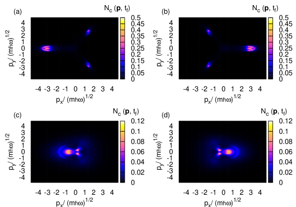
Figure 1: (Color online) Particle distribution function $N_{c}(\mathbf{p},t_{f})$ (in arbitrary units) after the interaction at the instant $t_{f}=20T$, as a function of scaled dimensionless momentum components is shown. The wave is assumed to be linearly polarized along the $y$ axis. Multiphoton excitation with the trigonal warping effect for the photon energy $\hbar\omega=E_{L}/1.1$ $\simeq$ $0.9$ $\mathrm{meV}$, the gap energy $U=4.05$ $\mathrm{meV}$ and the temperature $T/\hbar\omega=0.01$ are demonstrated at dimensionless intensity parameter $\chi=0.5$ for valleys (a) $\zeta=1$ and (b) $\zeta=-1$. In (c) and (d) corresponding to valleys $\zeta=1$ and $-1$, respectively, density plot of the distribution functions are shown for the photon energy $\hbar\omega$ $=$ $50$ $\mathrm{meV}\simeq 50E_{L}$, energy gap $U=250$ $\mathrm{meV}$, temperature $T/\hbar\omega=0.1$, and dimensionless parameter $\chi=1$.

As an initial state we assume an ideal Fermi gas in equilibrium with vanishing chemical potential and we will solve the set of Eqs. (18), (19), and (20) with the initial conditions:

$$P(\mathbf{p},0)=0;\ N_{c}(\mathbf{p},0)=\frac{1}{1+e^{\mathcal{E}_{1}\left(\mathbf{p}\right)/T}};$$ (21)

$$\ N_{\mathrm{v}}(\mathbf{p},0)=1-N_{c}(\mathbf{p},0).$$ (22)

Here $T$ is the temperature in energy units.

The components of the transition dipole moments are calculated via Eq. (13) by spinor wave functions (4):

$$D_{\mathrm{t}x}\left(\mathbf{p}\right)=-\frac{e\hbar}{2\mathcal{E}_{1}\left(\mathbf{p}\right)\sqrt{\mathcal{E}_{1}^{2}\left(\mathbf{p}\right)-\frac{U^{2}}{4}}}$$

$$\mathbf{\times}\left(\left[\left(\frac{p^{2}}{2m}-m\mathrm{v}_{3}^{2}\right)\frac{\zeta p_{y}}{m}+\frac{\mathrm{v}_{3}}{m}p_{x}p_{y}\right]\right.$$

$$\left.-i\frac{U}{2\mathcal{E}_{1}}\left\{\left(\frac{p^{2}}{2m}+m\mathrm{v}_{3}^{2}\right)\frac{p_{x}}{m}-\frac{3\zeta\mathrm{v}_{3}}{2m}\left(p_{x}^{2}-p_{y}^{2}\right)\right\}\right),$$ (23)

$$D_{\mathrm{t}y}\left(\mathbf{p}\right)=-\frac{e\hbar}{2\mathcal{E}_{1}\left(\mathbf{p}\right)\sqrt{\mathcal{E}_{1}^{2}\left(\mathbf{p}\right)-\frac{U^{2}}{4}}}$$

$$\times\left(\left[\left(-\frac{p^{2}}{2m}+m\mathrm{v}_{3}^{2}\right)\frac{\zeta p_{x}}{m}+\frac{\mathrm{v}_{3}}{2m}\left(p_{x}^{2}-p_{y}^{2}\right)\right]\right.$$

$$\left.-i\frac{U}{2\mathcal{E}_{1}}\left\{\left(\frac{p^{2}}{2m}+m\mathrm{v}_{3}^{2}\right)\frac{p_{y}}{m}+\frac{3\zeta\mathrm{v}_{3}}{m}p_{x}p_{y}\right\}\right).$$ (24)

The total mean dipole moments are

$$D_{x\mathrm{m}}\left(\mathbf{p}\right)=D_{x\mathrm{m}}\left(1,\mathbf{p}\right)-D_{x\mathrm{m}}\left(-1,\mathbf{p}\right)=-\frac{e\hbar U}{2\mathcal{E}_{1}\left(\mathbf{p}\right)\left(\mathcal{E}_{1}^{2}\left(\mathbf{p}\right)-\frac{U^{2}}{4}\right)}$$

$$\mathbf{\times}\left[\left(\frac{p^{2}}{2m}-m\mathrm{v}_{3}^{2}\right)\frac{\zeta p_{y}}{m}+\frac{\mathrm{v}_{3}}{m}p_{x}p_{y}\right],$$ (25)

$$D_{y\mathrm{m}}\left(\mathbf{p}\right)=D_{y\mathrm{m}}\left(1,\mathbf{p}\right)-D_{y\mathrm{m}}\left(-1,\mathbf{p}\right)==-\frac{e\hbar U}{2\mathcal{E}_{1}\left(\mathbf{p}\right)\left(\mathcal{E}_{1}^{2}\left(\mathbf{p}\right)-\frac{U^{2}}{4}\right)}$$

$$\times\left[\left(-\frac{p^{2}}{2m}+m\mathrm{v}_{3}^{2}\right)\frac{\zeta p_{x}}{m}+\frac{\mathrm{v}_{3}}{2m}\left(p_{x}^{2}-p_{y}^{2}\right)\right].$$ (26)

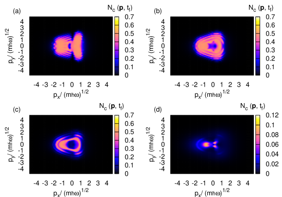
Figure 2: (Color online) Creation of a particle-hole pair in bilayer graphene at multiphoton resonant excitation. Particle distribution function $N_{c}(\mathbf{p},t_{f})$ (in arbitrary units) after the interaction is displayed at various gap energy: (a) $U=0$, (b) $U=75$ $\mathrm{meV}$, (c) $U=125$ $\mathrm{meV}$, and (d) $U=250$ $\mathrm{meV}$. The temperature is taken to be $T/\hbar\omega=0.1$. The wave is assumed to be linearly polarized along the $y$ axis with the frequency $\omega=$ $50$ $\mathrm{meV/\hbar}$ and intensity parameter is $\chi=1$. The results are for the valley $\zeta=1$.

Note that the matrix elements (23)-(26) are actually gauge dependent. Different choices of the basic function (4) (with the phase factor $e^{i\phi_{\sigma}(\mathbf{p})}$) will not change the energy spectrum (5), but will lead to the different dipole moments. Thus, inclusion of Berry connection (25), (26) into dynamics is mandatory for providing gauge invariance of the final results [29].

The set of equations (18), (19), and (20) can not be solved analytically. For the numerical solution we made a change of variables and transform the equations with partial derivatives into ordinary ones. The new variables are $t$ and $\widetilde{\mathbf{p}}=\mathbf{p}-\mathbf{p}_{E}$ $\left(t\right)$, where

$$\mathbf{p}_{E}\left(t\right)=-e\int_{0}^{t}\mathbf{E}\left(t^{\prime}\right)dt^{\prime}$$ (27)

is the classical momentum given by the wave field. After these transformations, the integration of equations (18), (19), and (20) is performed on a homogeneous grid of $10^{4}$ ($\widetilde{p}_{x},\widetilde{p}_{y}$)-points. For the maximal momentum we take $\widetilde{p}_{\max}/\sqrt{m\hbar\omega}=5$. The time integration is performed with the standard fourth-order Runge-Kutta algorithm. For the relaxation rate we take $\Gamma=0.5\mathcal{T}^{-1}$. The interaction parameters are chosen as follow. The wave-particle interaction at the photon energies $\hbar\omega>E_{L}$ for intraband transitions can be characterized by the dimensionless parameter $\chi=eE_{0}/(\omega\sqrt{m\hbar\omega})$, which is the ratio of the amplitude of the momentum given by the wave field to momentum at one-photon absorption. Here the intraband transitions are characterized by the classical momentum given by the wave field $\mathbf{p}_{E}\left(t\right)$. Besides, due to the gap the interband transitions will be characterized by the known Keldysh parameter [48]:

$$\gamma_{K}=\frac{\omega\sqrt{mU}}{eE_{0}}=\frac{1}{\chi}\sqrt{\frac{U}{\hbar\omega}},$$

which governs ionization process in the strong laser fields. For the considered case the ionization process reduces to the transfer of the electron from the valence band into the conduction band, in other words, to the creation of an electron-hole pair. It is obvious that interband transitions can be neglected when $\gamma_{K}>>1$. The latter means that wave field can not provide enough energy for the creation of an electron-hole pair and the generation of harmonics is suppressed. When $\gamma_{K}\sim 1$ or $\gamma_{K}<<1$ interband transitions take place. In the latter case, the transitions correspond to tunneling regime and are independent on the wave frequency. In the current paper, we will consider the optimal regime for the generation of harmonics $\gamma_{K}\sim 1$ and $\chi\sim 1$. Note that the intensity of the wave can be estimated as $I_{\chi}=\chi^{2}\times 6\times 10^{10}$ $Wcm^{-2}$ $(\hbar\omega/\mathrm{eV})^{3}$, so the required intensity $I_{\chi}$ for the nonlinear regime  strongly depends on the photon energy.

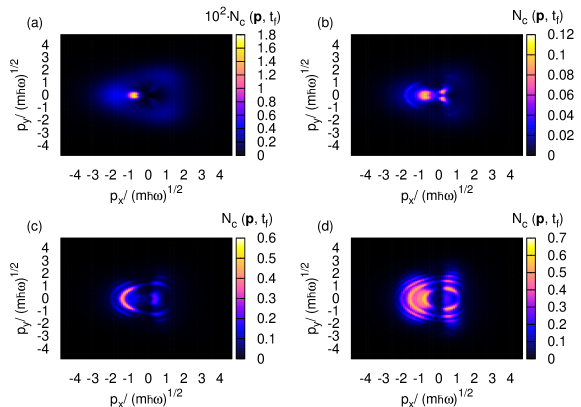
Figure 3: (Color online) Creation of a particle-hole pair in bilayer graphene at multiphoton excitation. Particle distribution function $N_{c}(\mathbf{p},t_{f})$ (in arbitrary units) after the interaction is displayed for various wave intensities. The temperature is taken to be $T/\hbar\omega=0.1$, and the band gap $U=250$ $\mathrm{meV}$. The wave is assumed to be linearly polarized along the $y$ axis with the frequency $\omega=$ $50$ $\mathrm{meV/\hbar}$. The results are for the valley $\zeta=1$: (a)–(d) correspond to dimensionless field parameters $\chi=0.5$, $1$, $1.5$, and $2$, respectively.

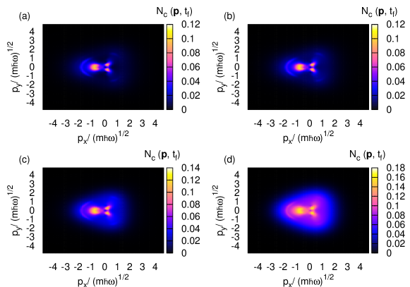
Figure 4: (Color online) Creation of a particle-hole pair in bilayer graphene at various temperatures and band gap $U=250$ $\mathrm{meV}$. Particle distribution function $N_{c}(\mathbf{p},t_{f})$ (in arbitrary units) the results for the valley $\zeta=1$ after the interaction are displayed for (a) $T/\hbar\omega=0.1$, (b) $T/\hbar\omega=0.3$, (c) $T/\hbar\omega=0.5$, and (d) $T/\hbar\omega=0.7$. The wave is assumed to be linearly polarized along the y axis with the frequency $\omega=$ $50$ $\mathrm{meV/\hbar}$ at wave intensity correspond to $\chi=1$.

Photoexcitations of the Fermi-Dirac sea are presented in Figs. 1–4. The wave is assumed to be linearly polarized along the $y$ axis. Similar calculations for a wave linearly polarized along the $x$ axis show qualitatively the same picture. In Fig.1 density plot of the particle distribution function $N_{c}(\mathbf{p},t_{f})$ is shown as a function of scaled dimensionless momentum components after the interaction. It is clearly seen the trigonal warping effect describing the deviation of the excited iso-energy contours from circles. Note that trigonal warping is crucial for even-order nonlinearity. In Fig. 2 the dependence of the photoexcitation of the Fermi-Dirac sea on the energy gap is shown. As is seen with the increasing of $U$ we approach to perturbative regime $\gamma_{K}>1$ and only weak excitation of Fermi-Dirac sea. In Fig. 3 we show the photoexcitation depending on the pump wave intensity. For the large values of $\chi$ when $\gamma_{K}=1.1$ we clearly see multiphoton excitations. With the increasing wave intensity, the states with absorption of more photons appear in the Fermi-Dirac sea. The multiphoton excitation of the Fermi-Dirac sea takes place along the trigonally warped isolines of the quasienergy spectrum modified by the wave field. Thus, the multiphoton probabilities of particle-hole pair production will have maximal values for the iso-energy contours defined by the resonant condition:

$$\frac{1}{\mathcal{T}}\int\limits_{0}^{\mathcal{T}}2\mathcal{E}_{1}\left(\widetilde{\mathbf{p}}+\mathbf{p}_{E}\left(t\right),t\right)dt=n\hbar\omega,\ \ n=1,2,3...,$$

These contours are also seen in Fig. 2. The temperature dependence of excitation of Fermi-Dirac sea is shown in Fig. 4. We see that excited isolines are slightly smeared out. This effect is small since $U>>$ $T$ and one can expect that harmonic spectra will be robust against temperature change in contrast to $U=0$ case where harmonics radiation is suppressed with the increase of temperature.

3 Generation of harmonics at the particle-hole multiphoton excitation

In this section we examine the nonlinear response of bilayer graphene considering nonadiabatic regime of harmonics generation when the Keldysh parameter is of the order of unity. For the coherent part of the radiation spectrum, one needs the mean value of the current density operator,

$$j_{\zeta}=-2e\left\langle\widehat{\Psi}(\mathbf{r},t)\left|\widehat{\mathbf{v}}_{\zeta}\right|\widehat{\Psi}(\mathbf{r},t)\right\rangle,$$ (28)

where $\widehat{\mathbf{v}}_{\zeta}=\partial\widehat{H}/\partial\widehat{\mathbf{p}}$ is the velocity operator and we have taken into account the spin degeneracy factor $2$. For the effective $2\times 2$ Hamiltonian (1) the velocity operator in components reads:

$$\widehat{\mathrm{v}}_{\zeta x}=\zeta\left(\begin{array}[]{cc}0&-\frac{1}{m}\left(\zeta\widehat{p}_{x}-i\widehat{p}_{y}\right)+\mathrm{v}_{3}\\ -\frac{1}{m}\left(\zeta\widehat{p}_{x}+i\widehat{p}_{y}\right)+\mathrm{v}_{3}&0\end{array}\right),$$ (29)

$$\widehat{\mathrm{v}}_{\zeta y}=i\left(\begin{array}[]{cc}0&\frac{1}{m}\left(\zeta\widehat{p}_{x}-i\widehat{p}_{y}\right)+\mathrm{v}_{3}\\ -\frac{1}{m}\left(\zeta\widehat{p}_{x}+i\widehat{p}_{y}\right)-\mathrm{v}_{3}&0\end{array}\right).$$ (30)

Using the Eqs. (28)–(30) and (15), the expectation value of the current for the valley $\zeta$ can be written in the form:

$$\mathbf{j}_{\zeta}\left(t\right)=-\frac{2e}{(2\pi\hbar)^{2}}\int d\mathbf{p}\left\{\mathbf{V}\left(\mathbf{p}\right)\left(N_{c}(\mathbf{p},t)-N_{\mathrm{v}}(\mathbf{p},t)\right)\right.$$

$$\left.+2\hbar^{-1}i\mathcal{E}_{1}\left(\mathbf{p}\right)\left[\mathbf{D}_{\mathrm{t}}\left(\mathbf{p}\right)P^{\ast}(\mathbf{p},t)-\mathbf{D}_{\mathrm{t}}^{\ast}\left(\mathbf{p}\right)P(\mathbf{p},t)\right]\right\},$$ (31)

where

$$\mathbf{V}\left(\mathbf{p}\right)=\frac{\mathrm{v}_{3}\mathbf{p}-3\zeta\frac{\mathrm{v}_{3}p}{2m}\mathbf{p}\cos 3\vartheta+3\zeta\frac{\mathrm{v}_{3}p^{3}}{2m}\sin 3\vartheta\frac{\partial\vartheta}{\partial\mathbf{p}}+2\frac{\mathbf{p}^{3}}{\left(2m\right)^{2}}}{\mathcal{E}_{1}\left(\mathbf{p}\right)}.$$ (32)

is the intraband velocity. As is seen from Eq. (31), the surface current provides two sources for the generation of harmonic radiation. The first term is the intraband current $\sim\left(N_{c}(\mathbf{p},t)-N_{\mathrm{v}}(\mathbf{p},t)\right)$. Intraband high harmonics are generated as a result of the independent motion of carriers in their respective bands. The second term in Eq. (31) describes high harmonics which are generated as a result of recombination of accelerated electron-hole pairs. Since we are in the nonadiabatic regimes, the contribution of both mechanisms are essential.

Figure 5: Third harmonic scaled emission rate ($G_{3}/\chi^{3}$) (in arbitrary units) for bilayer graphene versus $\chi$. The temperature is taken to be $T/\hbar\omega=0.1$, and the band gap $U=250$ $\mathrm{meV}$. The wave is assumed to be linearly polarized along the $y$ axis with the frequency $\omega=$ $50$ $\mathrm{meV/\hbar}$.

Since there is no degeneracy upon valley quantum number $\zeta$, the total current is obtained by a summation over $\zeta$:

$$j_{x}=j_{1,x}+j_{-1,x};$$ (33)

$$j_{y}=j_{1,y}+j_{-1,y}.$$ (34)

From Eq. (31) we see that

$$\frac{j_{x,y}}{j_{0}}=G_{x,y}\left(\omega t,\chi,\gamma_{K},\frac{\mathcal{E}_{L}}{\hbar\omega},\frac{T}{\hbar\omega}\right),$$ (35)

where

$$j_{0}=\frac{e\omega}{\pi^{2}}\sqrt{\frac{m\omega}{\hbar}},$$ (36)

and $G_{x}$ and $G_{y}$ are the dimensionless periodic (for monochromatic wave) functions, which parametrically depend on the interaction parameters $\chi$, $\gamma_{K}$, scaled Lifshitz energy, and temperature. Thus, having solutions of  Eqs. (18)-(20), and making an integration in Eq. (31), one can calculate the harmonic radiation spectra with the help of a Fourier transform of the function $G_{x,y}(t)$. The emission rate of the $n$th harmonic is proportional to $n^{2}|j_{n}|^{2}$, where $|j_{n}|^{2}$ = $|j_{xn}|^{2}$ + $|j_{yn}|^{2}$, with $j_{xn}$ and $j_{yn}$ being the $n$th Fourier components of the field-induced total current. To find $j_{n}$, the fast Fourier transform algorithm has been used. We have used the normalized current density (35) for the plots.

For clarification of the harmonics generation regime we first examine emission rate of the 3rd harmonic versus pump wave strength $\chi$, which is shown in Fig. 5.  As is seen from this figure, up to the field strengths $\chi<1$ we almost have power law ($\chi^{3}$) for the emission rate in accordance to perturbation theory. For large $\chi$ we have a strong deviation from power law for the emission rate of 3rd harmonic.

Figure 6: Harmonic emission rate in bilayer graphene at multiphoton excitation via $log_{10}(n^{2}|G_{n}|^{2})$ (in arbitrary units), as a function of the photon energy (in units of $\hbar\omega$), is shown for various gap energies. The temperature is taken to be $T/\hbar\omega=0.1$. The wave is assumed to be linearly polarized ($\phi=0$) with the intensity $\chi=1$ and frequency $\omega=$ $50$ $\mathrm{meV/\hbar}$. The results are for (a) $U=0$, (b) $U=75$ $\mathrm{meV}$, (c) $U=125$ $\mathrm{meV}$, and (d) $U=250$ $\mathrm{meV}$.

Figure 7: High harmonic spectra for bilayer graphene at multiphoton excitation is shown for various wave intensities in logarithmic scale. The temperature is taken to be $T/\hbar\omega=0.1$, the gap energy $U=250$ $\mathrm{meV}$. The wave is assumed to be linearly polarized ($\phi=0$) with the frequency $\omega=50$ $\mathrm{meV/\hbar}$. The results are for (a) $\chi=0.5$, (b) $\chi=1$, (c) $\chi=1.5$, and (d) $\chi=2$.

In Fig. 6 the dependence of the harmonic emission rate on the energy gap is shown. As is seen from this figure, in contrast to intrinsic bilayer graphene $U=0$ [16], when one has in plane inversion symmetry, here with the increasing of $U$ this symmetry is broken, and as a result, both even and odd harmonics are emitted. Besides, for the large $U$ due to the tunneling harmonics the cutoff is increased. In Fig. 7 high harmonic spectra for bilayer graphene at multiphoton excitation is shown for various wave intensities. As is seen, with the increasing wave intensity the high-order harmonics appear in the spectrum. The analysis also shows the linear dependence of the harmonics number cutoff on the amplitude of a pump electric field $n_{c}\sim\chi$. The temperature dependence of high harmonic radiation is clarified in Fig. 7, which shows the robustness of HHG in gapped graphene against temperature in contrast to intrinsic bilayer graphene [16], where harmonics are suppressed at high temperatures.

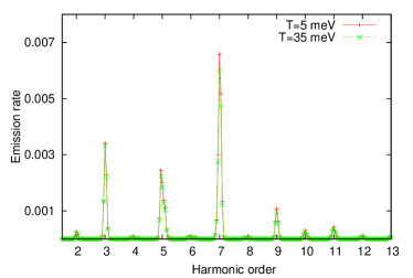
Figure 8: (Color online) High harmonic spectra for bilayer graphene at multiphoton excitation for a linearly polarized wave ($\phi=0$) is shown at $U=250$ $\mathrm{meV}$ for temperatures $T/\hbar\omega=0.7$ and $T/\hbar\omega=0.1$. The wave intensity $\chi=1$ and frequency $\omega=50$ $\mathrm{meV/\hbar}$.

Figure 9: High harmonic spectra in logarithmic scale for a elliptically polarized wave is shown at $U=250$ $\mathrm{meV}$ for temperature $T/\hbar\omega=0.1$ at the wave intensity $\chi=1$ and frequency $\omega=50$ $\mathrm{meV/\hbar}$. The results are for (a) $\phi=\pi/2$, (b) $\phi=\pi/4$, (c) $\phi=\pi/6$, and (d) $\phi=0$, respectively.

Finally in Fig. 9 we show the dependence of HHG on the polarization of the pump wave. The results are for linearly polarized wave along the $x$ ($\phi=\pi/2$) and $y$ ($\phi=0$) axes, for circular polarization ($\phi=\pi/4$) and for elliptic polarization ($\phi=\pi/6$). As is seen, orienting the linearly polarized pump wave along these axes results in different harmonics spectra. This is because we have strongly anisotropic excitation near the Dirac points. The difference is essential for even-order harmonics. For elliptic and circular polarizations the rates for the middle harmonics increase, while high order harmonics are suppressed.

4 Conclusion

We have presented the microscopic theory of nonlinear interaction of the gapped bilayer graphene with a strong coherent radiation field. The energy gap in considering case is produced by an electric field applied perpendicular to the bilayer graphene which breaks in plane inversion symmetry and is modifies the topology of bands. The closed set of differential equations for the single-particle density matrix is solved numerically for bilayer graphene in the Dirac cone approximation. For the pump wave, the THz frequency range has been taken. We have considered multiphoton excitation of Fermi-Dirac sea towards the high harmonics generation. It has been shown that the role of the gap in the nonlinear optical response of bilayer graphene is quite considerable. In particular, even-order nonlinear processes are present in contrast to intrinsic bilayer graphene, the cutoff of harmonics increases, and harmonic emission processes become robust against the temperature increase. The obtained results show that gapped bilayer graphene can serve as an effective medium for generation of even and odd high harmonics at room temperatures in the THz and far infrared domains of frequencies.

This work was supported by the RA MES State Committee of Science and Belarusian Republican Foundation for Fundamental Research (RB) in the frames of the joint research projects SCS AB16-19 and BRFFR F17ARM-25, accordingly.

References

References

• [1] Brabec T and Krausz F 2000Β Rev. Mod. Phys. 72 545
• [2] Avetissian H K 2016 Relativistic Nonlinear Electrodynamics: The QED Vacuum and Matter in Super-Strong Radiation Fields (New York: Springer)
• [3] Ferray M, L’Huillier A, Li X F, Lompre L A, Mainfray G, Manus C 1988Β Journal of Physics B 21 L31
• [4] Krausz F and Ivanov M 2009 Reviews of Modern Physics 81 163.
• [5] Smirnova O, Mairesse Y, Patchkovskii S, Dudovich N, Villeneuve D, Corkum P, and Ivanov M Yu 2009 Nature 460 972
• [6] Haessler S, Caillat J and Salieres P 2011 Journal of Physics B 44 203001
• [7] Wahlstram C G, Larsson J, Persson A, Starczewski T, Svanberg S, Salieres P, Balcou P and L’Huillier A 1993 Physical Review A 48 4709
• [8] Ghimire S, DiChiara A D, Sistrunk E, Agostini P, DiMauro L F, and Reis D A 2011 Nature Physics 7 138
• [9] Schubert O, Hohenleutner M, Langer F, Urbanek B, Lange C, Huttner U, Golde D, Meier T, Kira M, Koch S W, and Huber R 2014 Nature Photonics 8 119
• [10] Vampa G, Hammond T J, Thire N, Schmidt B E, Legare F, McDonald C R, Brabec T, and Corkum P B 2015 Nature 522 462
• [11] Ndabashimiye G, Ghimire S, Wu M, Browne D A, Schafer K J, Gaarde M B, and Reis D A 2016 Nature 534 520523
• [12] You Y S, Reis D A, and Ghimire S 2017 Nature Physics 13 345349
• [13] Liu H , Guo C, Vampa G, Zhang J L, Sarmiento T, Xiao M, Bucksbaum P H, Vuckovic J, Fan S, and Reis D A 2018 Nature Physics 14 1006
• [14] Mikhailov S A and Ziegler K 2008 J. Phys. Condens. Matter 20 384204
• [15] Avetissian H K, Avetissian A K, Mkrtchian G F, Sedrakian Kh V 2012 Phys. Rev. B 85 115443
• [16] Avetissian H K, Mkrtchian G F, Batrakov K G, Maksimenko S A, and Hoffmann A 2013 Phys. Rev. B 88 165411
• [17] Bowlan P, Martinez-Moreno E, Reimann K, Elsaesser T, and Woerner M 2014 Phys. Rev. B 89 041408
• [18] Al-Naib I, Sipe J E, and Dignam M M 2015 New J.Phys. 17 113018
• [19] Chizhova L A, Libisch F, and Burgdorfer J 2016 Phys. Rev. B 94 075412
• [20] Avetissian H K and Mkrtchian G F 2016 Phys. Rev. B 94 045419
• [21] Avetissian H K, Ghazaryan A G, Mkrtchian G F, and Sedrakian Kh V 2017 J. of Nanophotonics 11 016004
• [22] Chizhova L A, Libisch F, and Burgdorfer J 2017 Phys. Rev. B 95 085436
• [23] Dimitrovski D, Madsen L B, and Pedersen T G 2017 Phys. Rev. B 95 035405
• [24] Yoshikawa N, Tamaya T, and Tanaka K 2017 Science 356 736
• [25] Avetissian H K and Mkrtchian G F 2018 Phys. Rev. B 97 115454
• [26] Breton G Le, Rubio A, Tancogne-Dejean N 2018 Phys. Rev. B 98 165308
• [27] Liu H, Li Y, You Y S, Ghimire S, Heinz T F, Reis D A 2017 Nature Physics 13 262
• [28] Avetissian H K, Avetissian A K, Avchyan B R, Mkrtchian G F 2018 J. Phys. Condens. Matter 30 185302
• [29] Avetissian H K and Mkrtchian G F 2019 Phys. Rev. B 99 085432
• [30] Almalki S, Parks A M, Bart G, Corkum P B, Brabec T, and McDonald C R 2018 Phys. Rev. B 98 144307
• [31] Novoselov K S, Geim A K, Morozov S V, Jiang D, Zhang Y, Dubonos S V, Grigorieva I V, and Firsov A A 2004 Science 306 666
• [32] Castro Neto A H, Guinea F, Peres N M R, Novoselov K S, and Geim A K 2009 Rev. Mod. Phys. 81 540
• [33] Castro E V, Novoselov K S, Morozov S V, Peres N M R, Lopes dos Santos J M B, Nilsson J, Guinea F, Geim A K, and Neto A H C 2007 Phys. Rev. Lett. 99 216802
• [34] Zhang Y B, Tang T-T, Girit C, Hao Z, Martin M C, Zettl A, Crommie M F, Shen Y R, and Wan F 2009 Nature 459 820
• [35] Guinea F, Neto A H C, and Peres N M R 2006 Phys. Rev. B 73 245426
• [36] McCann E and Fal’ko V I 2006 Phys. Rev. Lett. 96 086805
• [37] Koshino M and Ando T 2006 Phys. Rev. B 73 245403
• [38] Abergel D S L and Chakraborty T 2009 Appl. Phys. Lett. 95 062107
• [39] Suarez Morell E and Torres Foa L E F 2012 Phys. Rev. B 86 125449
• [40] Dean J J and van Driel H M 2010 Phys. Rev. B 82 125411
• [41] Wu S, Mao L, Jones A M, Yao W, Zhang C, and Xu X 2012 Nano Lett. 12 2032
• [42] Ang Y S, Sultan S, and Zhang C 2010 Appl. Phys. Lett. 97 243110
• [43] Kumar N, Kumar J, Gerstenkorn C, Wang R, Chiu H-Y, Smirl A L, and Zhao H 2013 Phys. Rev. B 87 121406(R)
• [44] Aoki M and Amawashi H 2007 Solid State Commun. 142 123
• [45] Tang K, Qin R, Zhou J, Qu H, Zheng J, Fei R, Li H, Zheng Q, Gao Z, and Lu J 2011 J. Phys. Chem. C 115 9458
• [46] Xiao D, Chang M C, Niu Q 2010 Rev. Mod. Phys. 82 1959
• [47] Keldysh L V 1958 Sov. Phys.-JETP 7 788
• [48] Keldysh L V 1965 Sov. Phys.-JETP 20 1307
• [49] Lewenstein M, Balcou Ph, Ivanov M Yu, L’Huillier A, and Corkum P B 1994 Phys. Rev. A 49 2117
• [50] Cohen-Tannoudji C, Dupont-Roc J, and Grynberg G 1989 Photons and Atoms-Introduction to Quantum Electrodynamics (New York: Wiley)