Stochastic thermodynamics with arbitrary interventions

Abstract

We extend the theory of stochastic thermodynamics in three directions: (i) instead of a continuously monitored system we consider measurements only at an arbitrary set of discrete times, (ii) we allow for imperfect measurements and incomplete information in the description, and (iii) we treat arbitrary manipulations (e.g. feedback control operations) which are allowed to depend on the entire measurement record. For this purpose we define for a driven system in contact with a single heat bath the four key thermodynamic quantities: internal energy, heat, work and entropy along a single ‘trajectory’ for a causal model. The first law at the trajectory level and the second law on average is verified. We highlight the special case of Bayesian or ‘bare’ measurements (incomplete information, but no average disturbance) which allows us to compare our theory with the literature and to derive a general inequality for the estimated free energy difference in Jarzynksi-type experiments. An analysis of a recent Maxwell demon experiment using real-time feedback control is also given. As a mathematical tool, we prove a classical version of Stinespring’s dilation theorem, which might be of independent interest.

I Introduction

Stochastic thermodynamics has become a very successful theory to describe the thermodynamics of small, fluctuating systems arbitrarily far from equilibrium and even along a single stochastic trajectory (see Refs. Bustamante et al. (2005); Sekimoto (2010); Jarzynski (2011); Seifert (2012); Van den Broeck and Esposito (2015); Ciliberto (2017) for introductions and reviews). Its theoretical foundation rests on three pillars: (i) the system under study is continuously monitored, i.e. the time in between two observations is effectively zero; (ii) the system is perfectly measured, i.e. there is no uncertainty left in its state along a single trajectory; (iii) the system is only passively observed, i.e. no external interventions in form of disturbing measurements or feedback control operations are allowed.

To the best of the authors’ knowledge, no thorough study has been undertaken to overcome the first assumption, whereas a few interesting results have been obtained already to go beyond the second assumption, namely, incomplete information in the thermodynamic description of a stochastic system Ribezzi-Crivellari and Ritort (2014); Alemany et al. (2015); Bechhoefer (2015); García-García et al. (2016); Wächtler et al. (2016); Polettini and Esposito (2017, 2019). Beyond doubt, most progress has been achieved to incorporate feedback control, Maxwell’s demon and different sorts of information processing in the description (see Refs. Parrondo et al. (2015); Wolpert (2019) for an introduction). Nevertheless, many feedback scenarios, such as real-time or time-delayed feedback, are not covered by that framework.

Here, we will show how to overcome all three assumptions (i) – (iii) by following a recent proposal to build a consistent thermodynamic interpretation for a quantum stochastic process Strasberg (2018). More precisely, for a system, which is possibly driven by an external time-dependent force and in contact with a single heat bath, we will equip a causal model with a consistent thermodynamic framework. Causal models extend the standard notion of stochastic processes where an external agent (e.g. the experimenter) is not only passively observing a system, but where she is also allowed, e.g. to actively intervene in the process. This allows for a much richer theory where correlation and causation can be distinguished Pearl (2009). We suggest to call our novel framework operational stochastic thermodynamics to emphasize the fact that, from the perspective of the external agent, the control operations performed on the system are the primary objects of interest. Here, the notion ‘control operation’ is used in a wide sense and includes measurements, state preparations and feedback control operations, among other things. Only three rather standard assumptions are used here: first, in absence of any interventions or observations the system obeys the usual laws of thermodynamics; second, the system dynamics is Markovian; and third, the control operations of the external agent are idealized to happen instantaneously.

We note that first steps to combine stochastic thermodynamics and causal models have been already undertaken by Ito and Sagawa Ito and Sagawa (2013, 2016). There, stochastic thermodynamics was established for Bayesian networks, which are a particular representation of a causal model (here we will use a different one). A detailed comparison with their framework is postponed to later on.

Outline: As our framework requires to extend the usual notion of stochastic processes, Section II gives a brief self-contained introduction to the mathematical theory needed in the following including a classical version of Stinespring’s theorem. Section III then establishes the thermodynamic description of a causal model along a single trajectory and on average. While our theory is very general, it also appears quite abstract. Therefore, the special case of non-disturbing measurements, which is conventionally studied in the literature, is considered in Section IV. In there, we will show that our abstract framework allows us to draw physically relevant conclusions about, e.g. the estimated free energy differences in Jarzynski-type experiments Liphardt et al. (2002); Douarche et al. (2005); Gupta et al. (2011); Raman et al. (2014) or the second law in a recently realized “continuous Maxwell demon” experiment Ribezzi-Crivellari and Ritort (2019). Finally, we conclude with some remarks in Section V.

II Mathematical preliminaries

In classical physics, it is customary to assume that a system can be perfectly observed without disturbing it. If we label the elementary states of a physical system by $x$, then – by measuring the system at an arbitrary set of discrete times $t_{n}>\dots>t_{1}$ – we can infer the joint probability distribution $P(x_{n},\dots,x_{1})$ of finding the system in state $x_{n},\dots,x_{1}$ at the respective times $t_{n},\dots,t_{1}$. The assumption of a non-disturbing measurement implies the consistency condition

$$\sum_{x_{k}}P(x_{n},\dots,x_{k},\dots,x_{1})=P(x_{n},\dots,\cancel{x_{k}},\dots,x_{1}),$$ (1)

where the joint probability on the right hand side is obtained by measuring the system only at the times $t_{n}>\dots>t_{k+1}>t_{k-1}>\dots>t_{1}$ (i.e. there is no measurement at time $t_{k}$). Based on this consistency condition, the Daniell-Kolmogorov extension theorem guarantees that there is an underlying continuous time stochastic process which generates the joint probabilities $P(x_{n},\dots,x_{1})$ as its marginals. This is the foundational cornerstone for the theory of stochastic processes, which allows to bridge the discrepancy between experimental reality (where always only a finite amount of measurement data is available) and its theoretical description (where the mathematical description is usually provided in form of a differential equation, say a master equation).

In reality, however, an experimenter usually also influences a physical system. This can happen actively for a number of different reasons, e.g. to manipulate a system via feedback control, to prepare a certain state of the system, or to learn something about the process by unravelling its causal structure (for instance, to test the effect of a certain drug in a clinical trial one usually splits the patients into two groups: those who receive the drug and those who receive only placebos). The experimenter can also inactively influence a physical system, for instance, when the measurement adds an unwanted amount of noise to the system, which does not vanish on average. All those examples violate the consistency condition (1).

In Section II.1, we will review how to describe an arbitrary intervention or control operation performed at a single time. A causal model can then be seen as a set of control operations applied at different times to the system as reviewed in Section II.2. Finally, for our thermodynamic analysis it will be important that each control operation can be represented in terms of more primitive operations in a larger space. Quantum mechanically, this representation is provided by Stinespring’s theorem and in Section II.3 we will provide a classical analogue of it.

II.1 Control operations

As emphazised above, we view the terminology control operation in a broad sense, as any possible allowed state transformation applied to a physical system. The only requirement is that each control operation respects the statistical interpretation of the theory.

Before we come to the most general case, it is convenient to review Bayes’ theorem, which describes the limiting case of a ‘bare measurement’. By this we mean a measurement which is non-disturbing on average but not necessarily perfect. Let $p_{x}(t_{n}^{-})$ be the probability to find the system in state $x\in X$ (we consider for definiteness only a finite state space $X$) prior to the measurement at time $t_{n}$ (in general, by $t_{n}^{\pm}$ we will denote the time just before or after time $t_{n}$). Furthermore, let $P(r_{n}|x)$ be the conditional probability to obtain result $r_{n}$ in the measurement given that the system is in state $x$. The conditional state of the system after the measurement is then determined by Bayes’ rule,

$$p_{x}(t_{n}^{+},r_{n})=\frac{P(r_{n}|x)p_{x}(t_{n}^{-})}{P(r_{n})},$$ (2)

where the normalization factor $P(r_{n})=\sum_{x}P(r_{n}|x)p_{x}(t_{n}^{-})$ denotes the probability to obtain result $r_{n}$. In passing we note the slightly unusual notation with $p_{x}(t_{n}^{+},r_{n})$ denoting the conditional state of $X$ given the result $r_{n}$ [instead of using, maybe, $p_{t_{n}^{+}}(x|r_{n})$], which, however, turns out to be beneficial later on. Thus, whereas our state of knowledge changes along a single trajectory, i.e. $p_{x}(t_{n}^{+},r_{n})\neq p_{x}(t_{n}^{-})$, it does not change on average:

$$p_{x}(t_{n}^{+})=\sum_{r_{n}}P(r_{n})p_{x}(t_{n}^{+},r_{n})=p_{x}(t_{n}^{-}).$$ (3)

This is the essence of a non-disturbing measurement.

In turns out to be possible to generalize the above picture to the case where the classical control operation also changes the state of the system on average. This generalized description is indeed very close to quantum measurement theory Wiseman and Milburn (2010). For this purpose it is convenient to introduce the notion of a non-normalized system state $\tilde{p}_{x}(t_{n}^{+},r_{n})$, which allows to rewrite Bayes’ rule as

$$\tilde{p}_{x}(t_{n}^{+},r_{n})=\sum_{x^{\prime}}A_{x,x^{\prime}}(r_{n})p_{x^{\prime}}(t_{n}^{-}).$$ (4)

Here, in accordance with the notation used below, we have introduced the matrix $A(r_{n})$ with entries $A_{x,x^{\prime}}(r_{n})=\delta_{x,x^{\prime}}P(r_{n}|x)$. In terms of the vectors $\tilde{\textbf{p}}(t_{n}^{+},r_{n})$ and $\textbf{p}(t_{n}^{-})$ with entries $\tilde{p}_{x}(t_{n}^{+},r_{n})$ and $p_{x^{\prime}}(t_{n}^{-})$, respectively, the above can be compactly expressed as $\tilde{\textbf{p}}(t_{n}^{+},r_{n})=A(r_{n})\textbf{p}(t_{n}^{-})$. The only difference compared to Eq. (2) is then the missing normalization factor $P(r_{n})$. This, in fact, implies that Eq. (4) is linear with respect to the initial state of the system $p_{x}(t_{n}^{-},r_{n})$, which turns out to be convenient from a mathematical as well as numerical perspective. Furthermore, this step is of no harm, as the normalization factor is encoded in the non-normalized state by noting that $P(r_{n})=\sum_{x}\tilde{p}_{x}(t_{n}^{+},r_{n})=:\tau\tilde{\textbf{p}}(t_{n}^{+},r_{n})$, introducing the probability sum operator (‘trace’) $\tau$.

By generalizing this picture, every possible intervention will be described by a set of matrices $\{A(r_{n})=[A_{x,x^{\prime}}(r_{n})]\}$, which we call control operations. Each matrix $A(r_{n})$ describes the action of the experimenter based on a (generalized) measurement result $r_{n}$ according to Eq. (4). To preserve the positivity of the unnormalized state, every control operation is required to satisfy $A_{x,x^{\prime}}(r_{n})\geq 0$, but it does no longer need to be diagonal. Moreover, the average effect of the control operation is described by a single matrix $A\equiv\sum_{r_{n}}A(r_{n})$, i.e.  $\textbf{p}(t_{n}^{+})=A\textbf{p}(t_{n}^{-})$, because

$$p_{x}(t_{n}^{+})=\sum_{r_{n}}P(r_{n})p_{x}(t_{n}^{+},r_{n})=\sum_{x^{\prime}}A_{x,x^{\prime}}p_{x^{\prime}}(t_{n}^{-}).$$ (5)

To preserve the statistical interpretation of the theory, $A$ is required to be a stochastic matrix (meaning that each column is also normalized: $\sum_{x}A_{x,x^{\prime}}=1$ for all $x^{\prime}$). This describes the most general state transformation at the ensemble averaged level. Note that, in general, $p_{x}(t_{n}^{+})\neq p_{x}(t_{n}^{-})$.

Hence, to conclude, classical systems which are described by probability vectors can be manipulated by an arbitrary set of positive matrices $\{A(r_{n})\}$ with the sole requirement that they sum up to a stochastic matrix $A\equiv\sum_{r_{n}}A(r_{n})$.

II.2 Causal models

So far we focused on a single intervention happening at a single time $t_{n}$. A causal model can be seen as a prescription how to compute the effect of multiple interventions happening at a discrete set of times $t_{n}>\dots>t_{1}$ on the system. At each step some result $r_{k}$, $k\in\{1,\dots,n\}$, is obtained and we denote the entire sequence of measurement results by $\textbf{r}_{n}=(r_{n},\dots,r_{1})$ in the following. Given the outcome $r_{k}$, we assume that the experimenter knows which control operation $A(r_{k})$ she has implemented at time $t_{k}$. Moreover, we allow the experimenter to change her plan of interventions depending on the previous results $\textbf{r}_{k-1}$ and thus, we will write $A(r_{k}|\textbf{r}_{k-1})$ for the chosen control operation. Obviously, if the control operations describe bare measurements in the sense of Bayes’ rule, Eq. (2), and if we do not use the measurement results to manipulate the process, we recover the standard notion of a stochastic process. Causal models generalize this picture by allowing for any mathematically admissible control operation $A(r_{k}|\textbf{r}_{k-1})$.

To add some intrinsic time-evolution of the system to the picture, we will assume for simplicity and in view of our thermodynamic theory in Sec. III, that the system dynamics is Markovian. This means that the time-evolution in between two times $t_{k}$ and $t_{k+1}$ can be described by a transition matrix $T_{k+1,k}$, which propagates the system state forward in time:

$$\textbf{p}(t_{k+1})=T_{k+1,k}\textbf{p}(t_{k}).$$ (6)

Note that Markovianity implies that the transition matrix $T_{k+1,k}$ is well-defined independently on which state vector its act on. Mathematically, $T_{k+1,k}$ is nothing else than a stochastic matrix, but to emphasize its dynamical role we will call it a transition matrix. We will make no further assumption on $T_{k+1,k}$ here.

Now, let us denote by $\textbf{p}(t_{1}^{-})$ the initial state of the system (which can be arbitrary) prior to the first control operation. The unnormalized system state at time $t_{n}^{+}$ after the $n$’th control operation reads

$$\begin{split}\tilde{\textbf{p}}&(t_{n}^{+},\textbf{r}_{n})\\ &=A(r_{n}|\textbf{r}_{n-1})T_{n,n-1}\dots A(r_{2}|r_{1})T_{2,1}A(r_{1})\textbf{p}(t_{1}^{-}).\end{split}$$ (7)

In words, the state of the system given the measurement history $\textbf{r}_{n}$ is obtained by acting with the first control operation on it (obtaining result $r_{1}$), then letting the system evolve in time via $T_{2,1}$ until $t_{2}$, then applying the second control operation (obtaining result $r_{2}$), etc. until time $t_{n}^{+}$. Equivalently, we can express Eq. (7) iteratively,

$$\tilde{\textbf{p}}(t_{k}^{+},\textbf{r}_{k})=A(r_{k}|\textbf{r}_{k-1})T_{k,k-1}\tilde{\textbf{p}}(t_{k-1}^{+},\textbf{r}_{k-1}),$$ (8)

with $k\in\{2,\dots,n\}$ and $\tilde{\textbf{p}}(t_{1}^{+},r_{1})=A(r_{1})\textbf{p}(t_{1}^{-})$.

Finally, recall that each control operation can decrease the ‘trace’ of the system state and its value after the control operation is precisely the probability to obtain the respective measurement result. Applied to multiple control operations this means that the probability $P(\textbf{r}_{n})$ to obtain the sequence of results $\textbf{r}_{n}$ is

$$P(\textbf{r}_{n})=\tau\tilde{\textbf{p}}(t_{k}^{+},\textbf{r}_{k})=\sum_{x}\tilde{p}_{x}(t_{k}^{+},\textbf{r}_{n}).$$ (9)

Hence, the normalized system state after $n$ control operations is $\textbf{p}(t_{n}^{+},\textbf{r}_{n})=\tilde{\textbf{p}}(t_{n}^{+},\textbf{r}_{n})/P(\textbf{r}_{n})$ and the average system state at time $t_{n}^{+}$ reads

$$\textbf{p}(t_{n}^{+})=\sum_{\textbf{r}_{n}}P(\textbf{r}_{n})\textbf{p}(t_{n}^{+},\textbf{r}_{n}).$$ (10)

Here, we used the notational convention that an averaged quantity (with respect to the measurement results $\textbf{r}_{n}$) is denoted by simply dropping the dependence on $\textbf{r}_{n}$ in it [as in Eq. (3)].

To close this section, we remark that causal models can be also represented in different ways Pearl (2009) (see also Sec. IV.5) and the picture we have given here follows closely the description in the quantum case Pollock et al. (2018a, b); Milz et al. (2017). The particular and simple description (7) is a consequence of the Markov property Pollock et al. (2018a). Causal models can, however, also be defined for arbitrary non-Markovian systems, where the dynamics is more complicated but the control operations $A(r_{n}|\textbf{r}_{n-1})$ remain the essential ingredients Pollock et al. (2018b). A detailed comparison with classical causal models and the proof of a generalized extension theorem can be found in Ref. Milz et al. (2017).

II.3 A classical version of Stinespring’s theorem

This paper aims at providing a minimal, but consistent thermodynamic description for an arbitrary set of control operations. Obviously, as the control operations can be any possible state transformation, the resulting framework will on the most general level appear quite abstract. For instance, it is a priori not clear how to split the energetic changes caused by the action of some control operation $A(r)$ into work and heat. We will see that the following theorem helps us fix this issue, based only on the knowledge of $A(r)$. Moreover, it is indispensable for finding a valid second law during the control operation. Clearly, if additional knowledge about the experiment is available, telling us how the control operations are generated physically (knowledge which we assume not to have here), the present description should not necessarily be taken literally.

Moreover, we believe that the following theorem could be also useful for other applications. It tells us that any stochastic dynamics always arises from a reversible evolution in a larger space about which we have incomplete information. It is now commonly known as Stinespring’s theorem Stinespring (1955), but – to the best of our knowledge – there is no precise corresponding classical statement in the literature. We stress that the theorem, despite its similarity, does not automatically follow from its quantum version.

Theorem II.1.

Every stochastic matrix $A:\mathbb{R}^{d}\rightarrow\mathbb{R}^{d}$ can be represented as

$$A\textbf{p}=\bigl{(}(\operatorname{id}\otimes\tau)\circ\Pi\bigr{)}{\textbf{p}\otimes\textbf{q}},$$ (11)

where $\textbf{q}\in\mathbb{R}^{D}$ is a probability vector with a dimension $D\leq d(d^{2}-d+1)$ and $\Pi:\mathbb{R}^{d}\otimes\mathbb{R}^{D}\rightarrow\mathbb{R}^{d}\otimes\mathbb{R}^{D}$ is a permutation matrix. Recall that $\tau$ is the marginal (‘trace’) operator. In terms of the matrix elements, the above equation expands to

$$A_{x,x^{\prime}}=\sum_{y,y^{\prime}=1}^{D}\Pi_{xy,x^{\prime}y^{\prime}}q_{y^{\prime}}.$$

Moreover, for an arbitrary decomposition of $A$ into a set of control operations, $A(r)$ such that $A_{x,x^{\prime}}(r)\geq 0$ for all $x,x^{\prime}$ and $r$, we can write

$$A(r)\textbf{p}=\bigl{[}[\operatorname{id}\otimes\tau B(r)]\circ\Pi\bigl{]}{\textbf{p}\otimes\textbf{q}},$$ (12)

meaning

$$A_{x,x^{\prime}}(r)=\sum_{y,y^{\prime}=1}^{D}B_{y,y}(r)\Pi_{xy,x^{\prime}y^{\prime}}q_{y^{\prime}},$$

where $B(r)$ describes the effect of a bare measurement: all $B(r)$ are diagonal, non-negative matrices, whose sum is the identity matrix. The permutation matrix $\Pi$ and the probability vector q in Eq. (12) are the same as in Eq. (11).

In words, any stochastic evolution of a system can be seen as arising from marginalizing a reversible evolution in a larger ‘system-ancilla’ space. The ancilla, initially described by the probabilities $q_{y}$, is a priori only an auxiliary system without physical meaning. Often, however, it can be connected to a part of the real physical environment, for instance a detector or memory which is used to record the outcome of a measurement. Furthermore, any ‘selective’ evolution conditioned on a generalized measurement result $r$ can be modeled by an ideal bare (or ‘Bayesian’) measurement acting on this ancilla state only. This nicely encodes the fact that an experimenter usually never observes the system directly, but rather infers its state by looking at a secondary object, e.g. a display, which in turn is not affected by the observation.

A proof of Theorem II.1 is given in the Appendix, where we also show that the minimum dimension $D$ of the extra space is in general strictly smaller than $d(d^{2}-d+1)$. We do not know how to characterize the minimum $D$, except as a non-trivial optimization problem.

Finally, to complete this digression, let us compare the classical with the quantum version of the theorem. Quantum mechanically, instead of using a stochastic matrix, one describes the dissipative evolution of a system by a completely positive and trace-preserving (cptp) map. In the extended system-ancilla space, $P$ becomes a unitary matrix and the dimension $D$ can be fixed to be $d^{2}$ (where $d$ denotes the dimension of the system Hilbert space). Crucially, the initial state of the ancilla can be always chosen to be a pure state, in which case the minimum $D$ is the so-called Kraus rank of the cptp map, which coincides with the matrix rank of its Choi matrix. Especially the last point is in strong contrast to the classical version of the theorem, where a pure ancilla state can never suffice.

III Operational stochastic thermodynamics

We now turn to the physical situation we wish to study and understand thermodynamically. We consider systems described by a finite set of states $\{x\}$, whose dynamics is described by a rate master equation

$$\frac{{\mathrm{d}}}{{\mathrm{d}}t}p_{x}(t)=\sum_{x^{\prime}}W_{x,x^{\prime}}(\lambda_{t})p_{x^{\prime}}(t).$$ (13)

Here, $W(\lambda_{t})$ is a rate matrix obeying $\sum_{x}W_{x,x^{\prime}}(\lambda_{t})=0$ and $W_{x,x^{\prime}}(\lambda_{t})\geq 0$ for all $x\neq x^{\prime}$. In terms of the probability vector $\textbf{p}(t)$, the above can be stated compactly as $\frac{{\mathrm{d}}}{{\mathrm{d}}t}\textbf{p}(t)=W(\lambda_{t})\textbf{p}(t)$.

As evidenced in the notation, $W$ is allowed to depend on an external control parameter $\lambda_{t}$, which can change in time. Physically speaking, such a time-dependence arises from manipulating the free energy landscape of the system. To each state $x$ we will thus associate a free energy $f_{x}(\lambda_{t})=e_{x}(\lambda_{t})-Ts_{x}(\lambda_{t})$, where $T$ is the temperature of the surrounding heat bath and $e_{x}(\lambda_{t})$ and $s_{x}(\lambda_{t})$ are the internal energy and the intrinsic entropy of state $x$, respectively. The intrinsic entropy arises because $x$ is not necessarily a ‘single microstate’ in a Hamiltonian sense, but could be an effective mesostate obtained from coarse-graining over a set of microstates (e.g. many microscopic configurations of a molecule can give raise to the same conformational state), see also Refs. Seifert (2011); Esposito (2012). Furthermore, we assume that the rates satisfy local detailed balance,

$$\frac{W_{x,x^{\prime}}(\lambda_{t})}{W_{x^{\prime},x}(\lambda_{t})}=e^{-\beta[f_{x}(\lambda_{t})-f_{x^{\prime}}(\lambda_{t})]},$$ (14)

where $\beta=T^{-1}$ (we set $k_{B}\equiv 1$). This condition allows us to link changes in the system state to entropic changes in the bath. We define the following key thermodynamic quantities. First, the internal energy is

$$U(t)\equiv\sum_{x}e_{x}(\lambda_{t})p_{x}(t)=\textbf{e}(\lambda_{t})\cdot\textbf{p}(t),$$ (15)

which we have expressed as a scalar product for later convenience. Then, the heat flux and power are

$$\dot{Q}(t) \equiv\textbf{e}(\lambda_{t})\cdot\frac{d\textbf{p}(t)}{dt},$$ (16)

$$\dot{W}(t) \equiv\frac{d\textbf{e}(\lambda_{t})}{dt}\cdot\textbf{p}(t),$$ (17)

such that the first law takes on the familiar form

$$\frac{d}{dt}U(t)=\dot{Q}(t)+\dot{W}(t).$$ (18)

Furthermore, the system entropy reads

$$\begin{split}S_{S}(t)&\equiv\sum_{x}p_{x}(t)[-\ln p_{x}(t)+s_{x}(\lambda_{t})]\\ &=S_{\text{Sh}}\left[\{p_{x}(t)\}_{x}\right]+\textbf{s}(\lambda_{t})\cdot\textbf{p}(t),\end{split}$$ (19)

where $S_{\text{Sh}}\left[\{p_{x}(t)\}_{x}\right]\equiv-\sum_{x}p_{x}(t)\ln p_{x}(t)$ denotes the Shannon entropy. Then, the second law of nonequilibrium thermodynamics becomes

$$\dot{\Sigma}(t)=\frac{d}{dt}S_{S}(t)-\beta Q(t)-\frac{\partial\textbf{s}(\lambda_{t})}{\partial t}\cdot\textbf{p}(t)\geq 0,$$ (20)

where the reversible change in intrinsic entropy needs to be substracted as it also appears in the time-derivative of the system entropy (19) Seifert (2011); Esposito (2012). Furthermore, $\dot{\Sigma}(t)$ denotes the entropy production rate. We emphasize that the present setup covers a large class of systems studied in stochastic thermodynamics Bustamante et al. (2005); Sekimoto (2010); Jarzynski (2011); Seifert (2012); Van den Broeck and Esposito (2015); Ciliberto (2017). What is, however, unclear at present is how to incorporate multiple heat reservoirs into the description.

The goal of the present paper can now be formulated at follows. We consider a system, which evolves according to a Markovian rate master equation as above. Furthermore, we assume it obeys the laws of thermodynamics as specified above at the unmeasured level (i.e. without any sort of interventions). Now, we seek for a consistent set of definitions of internal energy, heat, work and entropy along a single trajectory for an arbitrary causal model as described in Section II, see in particular Eq. (7). Note that here we take an explicitly observer-dependent point of view: any action (including measurements) must be explicitly modelled within our framework, no further ‘hidden’ knowledge is used. A ‘single trajectory’ is therefore defined by the sequence of measurement results $\textbf{r}_{n}$, which, in general, refers to a discrete set of times and can include arbitrary generalized measurements. In view of Eq. (13) the transition matrices in Eq. (7) are given by

$$T_{k,j}\equiv{\cal{T}}_{+}\exp\left[\int_{t_{j}}^{t_{k}}W(\lambda_{t})dt\right]$$ (21)

with the time-ordering operator ${\cal{T}}_{+}$. Furthermore, albeit implicit in the notation, we also allow the control protocol $\lambda_{t}=\lambda_{t}(\textbf{r}_{n})$ ($t\geq t_{n}$) to depend on all previous measurement outcomes. Thus, we can treat all conceivable feedback scenarios within our framework.

We remark that the sole assumptions behind the dynamical description (7) are that the system as described by Eq. (13) is Markovian (but see Refs. Strasberg and Esposito (2019); Strasberg (2019) for extensions) and that the external agent effectively implements the control operations instantaneously, which ensures that she has full control over them. To derive a consistent thermodynamic interpretation for a causal model, we will use Theorem II.1 and model explicitly the stream of ancilla systems interacting sequentially with the system, similar to the repeated interaction framework in Refs. Strasberg et al. (2017); Strasberg (2018).

III.1 First law

In between two control operations, the first law is simply given by

$$\frac{{\mathrm{d}}}{{\mathrm{d}}t}U(t,\textbf{r}_{n-1})=\dot{Q}(t,\textbf{r}_{n-1})+\dot{W}(t,\textbf{r}_{n-1}).$$ (22)

This is essentially Eq. (18), only that here we have explicitly emphasized that all quantities can depend on the entire measurement record $\textbf{r}_{n-1}$, either because the state at time $t_{n-1}$ or the control protocol $\lambda_{t}$ (or both) depend on it. The time-interval of validity, $t_{n-1}<t<t_{n}$, is unambiguously indicated by the index on the sequence $\textbf{r}_{n-1}$.

Through the control operation at time $t_{n}$, non-trivial changes may happen, as the internal energy can jump:

$$\Delta U^{\text{ctrl}}(\textbf{r}_{n})=\textbf{e}(\lambda_{t})\cdot\left[\frac{A(r_{n}|\textbf{r}_{n-1})}{P(r_{n}|\textbf{r}_{n-1})}-\operatorname{id}\right]\textbf{p}(t_{n}^{-},\textbf{r}_{n-1}).$$ (23)

Notice that we are careful to use the normalized system state here. Hence, we needed to normalize the system state after the control operation by using the conditional probability $P(r_{n}|\textbf{r}_{n-1})\equiv P(\textbf{r}_{n})/P(\textbf{r}_{n-1})$. To attribute to each control operation a meaningful heat and work, we make use of Theorem II.1. The representation (12), where the action of an arbitrary control operation is split into a reversible, deterministic part (the permutation matrix $\Pi$) and an irreversible, non-deterministic part (the bare measurement $B$), strongly suggest to associate changes caused by the first part as work and changes caused by the second part as heat Elouard et al. (2017); Strasberg (2018). However, in contrast to the quantum case we have to be more careful here as we are not only changing the energy of the system, but also its instrinsic entropy. Therefore,

$$\begin{split}W&{}^{\text{ctrl}}(t_{n},\textbf{r}_{n-1})\equiv\\ &\textbf{f}(\lambda_{t})\cdot\left\{\bigl{(}(\operatorname{id}\otimes\tau)\circ\Pi\bigr{)}\textbf{p}(t_{n}^{-},\textbf{r}_{n-1})\otimes\textbf{q}-\textbf{p}(t_{n}^{-},\textbf{r}_{n-1})\right\},\end{split}$$ (24)

which describes the change in the system’s free energy due to the reversible and deterministic permutation. Note that we suppressed in the notation that the choice of the initial ancilla state $\textbf{q}=\textbf{q}(\textbf{r}_{n-1})$ and of the permutation matrix $\Pi=\Pi(\textbf{r}_{n-1})$ can depend on previous measurement results $\textbf{r}_{n-1}$. However, due to causality they can not depend on the actual outcome $r_{n}$ obtained at time $t_{n}$, and therefore the work does not depend on it, either. In fact, the work during the control operation can be computed by knowing only the state after the control operation averaged over the last measurement result, which is

$$\begin{split}\textbf{p}(t_{n}^{+},\textbf{r}_{n-1})&=\sum_{r_{n}}P(r_{n}|\textbf{r}_{n-1})\textbf{p}(t_{n}^{+},\textbf{r}_{n})\\ &=\bigl{(}(\operatorname{id}\otimes\tau)\circ\Pi\bigr{)}\textbf{p}(t_{n}^{-},\textbf{r}_{n-1})\otimes\textbf{q}\\ &=\sum_{r_{n}}A(r_{n}|\textbf{r}_{n-1})\textbf{p}(t_{n}^{-},\textbf{r}_{n-1}).\end{split}$$ (25)

Hence, the work is uniquely determined by the average control operation $A_{n}\equiv\sum_{r_{n}}A(r_{n}|\textbf{r}_{n-1})$ (we again suppressed the dependence on $\textbf{r}_{n-1}$ for notational convenience) and the system state before the control operation. This can be compactly expressed as:

$$W^{\text{ctrl}}(t_{n},\textbf{r}_{n-1})=\textbf{f}(\lambda_{t})\cdot(A_{n}-\operatorname{id})\textbf{p}(t_{n}^{-},\textbf{r}_{n-1}),$$ (26)

Next, the heat injected during the control operation is demanded to fulfill the first law of thermodynamics $Q^{\text{ctrl}}(t_{n},\textbf{r}_{n})=\Delta U^{\text{ctrl}}(\textbf{r}_{n})-W^{\text{ctrl}}(t_{n},\textbf{r}_{n-1})$. Hence, it is given by

$$\begin{split}Q^{\text{ctrl}}(t_{n},\textbf{r}_{n})=&~{}\textbf{e}(\lambda_{t})\cdot\left[\frac{A(r_{n}|\textbf{r}_{n-1})}{P(r_{n}|\textbf{r}_{n-1})}-A_{n}\right]\textbf{p}(t_{n}^{-},\textbf{r}_{n-1})\\ &+T\textbf{s}(\lambda_{t})\cdot(A_{n}-\operatorname{id})\textbf{p}(t_{n}^{-},\textbf{r}_{n-1}).\end{split}$$ (27)

Thus, the heat depends on the last measurement result $r_{n}$ at the trajectory level. Averaging over it, we confirm that

$$\begin{split}\sum_{r_{n}}&P(r_{n}|\textbf{r}_{n-1})Q^{\text{ctrl}}(t_{n},\textbf{r}_{n})\\ &=T\textbf{s}(\lambda_{t})\cdot(A_{n}-\operatorname{id})\textbf{p}(t_{n}^{-},\textbf{r}_{n-1}).\end{split}$$ (28)

Finally, we remark that we have assumed that the states $y$ of the ancilla are energetically neutral and thus do not contribute to the energy balance. This is indeed the conventional choice when considering Maxwell demon feedbacks, where – as we will see – the memory of the demon can be identified with the ancilla. The generalization to energetically non-neutral ancillas is straightforward Strasberg (2018) and will not be considered here.

To summarize, over an interval denoted by a superscript $(n]$, which starts at time $t_{n-1}^{+}$, just after the $(n-1)$-st control operation and ends at time $t_{n}^{+}$, just after the $n$-th control operation, the first law at the trajectory level can be written as usual

$$\Delta U^{(n]}(\textbf{r}_{n})=Q^{(n]}(\textbf{r}_{n})+W^{(n]}(\textbf{r}_{n-1}),$$ (29)

but each term is now composed out of a part referring to the unobserved evolution [Eq. (22)] and to the control operation [Eq. (23)], e.g.

$$W^{(n]}(\textbf{r}_{n-1})=\int_{t_{n-1}^{+}}^{t_{n}^{-}}dt\dot{W}(t,\textbf{r}_{n-1})+W^{\text{ctrl}}(\textbf{r}_{n-1}).$$ (30)

The first law over multiple time-intervals can be obtained by concatenating the first laws for each time-interval.

III.2 Stochastic entropy

Whereas we did not need to redefine the notion of internal energy, but could simply apply Eq. (15) with respect to the conditional state of the system, it turns out to be necessary to redefine the entropy of the system, explicitly taking into account the external ancillas and the generated measurement record, too. In fact, as we allow our control protocol to depend on the entire measurement record, it is important to store also all available information about the past. Thus, let us denote by $p_{x,\textbf{y}_{n}}(t,\textbf{r}_{n})$ the joint probability, conditioned on $\textbf{r}_{n}$, to find the system in state $x$ and the stream of ancillas in state $\textbf{y}_{n}=(y_{n},\dots,y_{1})$, where $y_{k}$ denotes the state of the ancilla responsible for the $k$-th control operation. Then, we define

$$\begin{split}S(t,\textbf{r}_{n})\equiv&~{}S_{\text{Sh}}\left[\{p_{x,\textbf{y}_{n}}(t,\textbf{r}_{n})\}_{x,\textbf{y}_{n}}\right]\\ &+\textbf{s}(\lambda_{t})\cdot\textbf{p}(t,\textbf{r}_{n})-\ln P(\textbf{r}_{n}).\end{split}$$ (31)

The entropy of the system along a particular trajectory is given by three terms. The first terms describes nothing but the remaining uncertainty about the system and ancilla state, which is quantified by the Shannon entropy, as usual. The second term simply denotes the average intrinsic entropy conditioned on the measurement results. The third term describes the stochastic uncertainty left about the measurement outcomes $\textbf{r}_{n}$. When averaged over the probability $P(\textbf{r}_{n})$ to obtain the results $\textbf{r}_{n}$, it gives the usual Shannon entropy of the measurement outcomes. Two important remarks are in order:

First, while the definition (31) looks quite cumbersome in general, in can often be significantly simplified. For instance, when the final measurement of the ancilla system is perfect, then the information content stored in all ancillas is identical to the information content of the measurement results because

$$p_{x,\textbf{y}_{n}}(t,\textbf{r}_{n})=p_{x}(t,\textbf{r}_{n})\delta_{y_{n},r_{n}}\dots\delta_{y_{1},r_{1}}$$ (32)

for $t>t_{n}$. If the ancillas are also prepared in a zero entropy state, $S_{\text{Sh}}(\textbf{q})=0$, then Eq. (31) reduces for all times to

$$S(t,\textbf{r}_{n})=S_{\text{Sh}}[\textbf{p}(t,\textbf{r}_{n})]+\textbf{s}(\lambda_{t})\cdot\textbf{p}(t,\textbf{r}_{n})-\ln P(\textbf{r}_{n}).$$ (33)

Furthermore, let us consider the case in which the measurement is perfect such that we have complete information about the system state. Then, $S_{\text{Sh}}[\textbf{p}(t_{n}^{+},\textbf{r}_{n})]=0$ and if we also set $\textbf{s}(\lambda_{t})=0$ for simplicity, we obtain the important limit

$$S(t_{n}^{+},\textbf{r}_{n})=-\ln P(\textbf{r}_{n}).$$ (34)

We are now in a position to compare our definition with the conventional one Seifert (2005), which is $-\ln p(x_{t})$ where $p(x_{t})$ is the probability to find the system in state $x$ at time $t$ as determined by the master equation (13). Undeniably, this definition has turned out to be very successful and we do not want to question it per se within the traditional scope of stochastic thermodynamics. Nevertheless, it is conceptionally not fully satisfactory. If we are confident that Shannon entropy is the correct thermodynamic entropy to describe a small system in contact with a large bath and if we have perfect knowledge about the system state, then its Shannon entropy should be zero and not $-\ln p(x_{t})\neq 0$. Furthermore, if information is really physical Landauer (1991), then it matters whether we measure a system or not. Thus, when we average the standard definition $-\ln p(x_{t})$, we neglect a large part of the entropy production, which is generated in the memory of the measurement apparatus.

We therefore believe that our definition (31) fills an important conceptual gap in stochastic thermodynamics. First, it reassures us that Shannon entropy is the correct thermodynamic entropy for a small system as considered here. Second, it tells us that within the conventional (perfect measurement) limit of stochastic thermodynamics, the stochastic entropy is not $-\ln p(x_{t})$, but actually $-\ln p(r_{n})$. Both terms agree numerically at time $t=t_{n}^{+}$, but the latter corresponds to the stochastic entropy generated in the memory. This should be compared with our notion (34) in the perfect measurement limit, which solely differs by explicitly accounting for the entropy generated in the entire memory. In the following we will also refer to Eq. (31) as ‘stochastic entropy’: it is an entropy defined along a single trajectory and, as we will now see, gives rise to an always positive entropy production when averaged.

III.3 Second law

The second law in the absence of any control operation follows basically from Eq. (20), where all quantities can now depend on the measurement record $\textbf{r}_{n-1}$ as we are working at the trajectory level. Specifically,

$$\begin{split}\dot{\Sigma}(t,\textbf{r}_{n-1})=&~{}\frac{d}{dt}S(t,\textbf{r}_{n-1})-\beta Q(t,\textbf{r}_{n-1})\\ &-\frac{\partial\textbf{s}(\lambda_{t})}{\partial t}\cdot\textbf{p}(t,\textbf{r}_{n-1})\\ \geq&~{}0\end{split}$$ (35)

Note, however, that here we used our definition (31) and not Eq. (19), which differs by taking into account the entropy of the ancillas and the system-ancilla correlations. Positivity of Eq. (35) is nevertheless ensured as the transition matrices $T_{k,j}$ of Eq. (21) act only locally on the system. Hence, they do not change the entropy of the ancillas and can only decrease the system-ancilla correlations. Proving this statement follows identical steps as in Ref. Strasberg (2018); compare also with the “modularity cost” of Ref. Boyd et al. (2018).

The more interesting part concerns the entropy production during the control step, which we define as

$$\Sigma^{\text{ctrl}}(t_{n},\textbf{r}_{n})\equiv\Delta S^{\text{ctrl}}(t_{n},\textbf{r}_{n})-\beta Q^{\text{ctrl}}(t_{n},\textbf{r}_{n}),$$ (36)

where $\Delta S^{\text{ctrl}}(t_{n},\textbf{r}_{n})\equiv S(t_{n}^{+},\textbf{r}_{n})-S(t_{n}^{-},\textbf{r}_{n-1})$ denotes the change in entropy due to the control operation. Note that we assume that the control operations happens instantaneously such that $\lambda_{t}$ does not vary around $t=t_{n}$. This implies that there is no reversible change in intrinsic entropy, which could contribute to the entropy production. It remains to be shown that the entropy production is positive on average, i.e.

$$\sum_{r_{n}}P(r_{n}|\textbf{r}_{n-1})\Sigma^{\text{ctrl}}(t_{n},\textbf{r}_{n})\geq 0.$$ (37)

This then implies $\sum_{\textbf{r}_{n}}P(\textbf{r}_{n})\Sigma^{\text{ctrl}}(t_{n},\textbf{r}_{n})\geq 0$, too. To prove Eq. (37), we first notice that due to Eq. (28) and $-\ln P(\textbf{r}_{n})+\ln P(\textbf{r}_{n-1})=\ln P(r_{n}|\textbf{r}_{n-1})$ we have

$$\begin{split}\sum_{r_{n}}P(r_{n}|\textbf{r}_{n-1})\Sigma^{\text{ctrl}}(t_{n},\textbf{r}_{n})&=\sum_{r_{n}}P(r_{n}|\textbf{r}_{n-1})S_{\text{Sh}}\left[\bigl{\{}p_{x,\textbf{y}_{n}}(t_{n}^{+},\textbf{r}_{n})\bigr{\}}_{x,\textbf{y}_{n}}\right]\\ &\phantom{===}+S_{\text{Sh}}\left[\bigl{\{}P(r_{n}|\textbf{r}_{n-1})\bigr{\}}_{r_{n}}\right]-S_{\text{Sh}}\left[\bigl{\{}p_{x,\textbf{y}_{n}}(t_{n}^{-},\textbf{r}_{n-1})\bigr{\}}_{x,\textbf{y}_{n}}\right].\end{split}$$ (38)

This expression characterizes the change in informational entropy of the system, the ancilla and the $n$-th measurement record during the control operation. We then use Eqs. (11) and (12) to write the unnormalized state of the system and all ancillas after the control operation as

$$\tilde{p}_{x,\textbf{y}_{n}}(t_{n}^{+},\textbf{r}_{n})=P(r_{n}|\textbf{r}_{n-1})p_{x,\textbf{y}_{n}}(t_{n}^{+},\textbf{r}_{n})=\sum_{x^{\prime},y^{\prime}_{n}}B_{y_{n},y_{n}}(r_{n}|\textbf{r}_{n-1})\Pi_{xy_{n},x^{\prime}y_{n}^{\prime}}(\textbf{r}_{n-1})p_{x^{\prime},y_{n}^{\prime}\textbf{y}_{n-1}}(t_{n}^{-},\textbf{r}_{n-1}).$$ (39)

Note that both the permutation matrix $\Pi$ and the bare measurement $B(r_{n})$ can depend on $\textbf{r}_{n-1}$ if $A(r_{n}|\textbf{r}_{n-1})$ depends on it. Now recall that the Shannon entropy is invariant under permutations and that the bare measurement in Eq. (39), when summed over the outcomes $r_{n}$, has no effect. Thus,

$$\begin{split}&S_{\text{Sh}}\left[\bigl{\{}p_{x,y_{\textbf{n}}}(t_{n}^{-},\textbf{r}_{n-1})\bigr{\}}_{x,\textbf{y}_{n}}\right]\\ &=S_{\text{Sh}}\left[\left\{\sum_{x^{\prime},y^{\prime}_{n}}\Pi_{xy_{n},x^{\prime}y^{\prime}_{n}}p_{x^{\prime},y_{n}^{\prime}\textbf{y}_{n-1}}(t_{n}^{-},\textbf{r}_{n-1})\right\}_{\!\!x,\textbf{y}_{n}}\right]\\ &=S_{\text{Sh}}\left[\left\{\sum_{r_{n}}P(r_{n}|\textbf{r}_{n-1})p_{x,\textbf{y}_{n}}(t_{n}^{+},\textbf{r}_{n})\right\}_{\!\!x,\textbf{y}_{n}}\right].\end{split}$$ (40)

The term $P(r_{n}|\textbf{r}_{n-1})p_{x,\textbf{y}_{n}}(t_{n}^{+},\textbf{r}_{n})$ can be viewed as a joint probability distribution over the probability space of the system, the ancilla and the $n$-th measurement record. But for any bipartite probability distribution $\{p_{ab}\}_{ab}$ with marginal $\{p_{a}=\sum_{b}p_{ab}\}_{a}$, we have the inequality $S_{\text{Sh}}[\{p_{a}\}_{a}]\leq S_{\text{Sh}}[\{p_{ab}\}_{ab}]$. Hence, Eq. (37) is proved by noting that

$$\begin{split}S_{\text{Sh}}&\left[\bigl{\{}p_{x,\textbf{y}_{n}}(t_{n}^{-},\textbf{r}_{n-1})\bigr{\}}_{x,\textbf{y}_{n}}\right]\\ &\leq S_{\text{Sh}}\left[\bigl{\{}P(r_{n}|\textbf{r}_{n-1})p_{x,\textbf{y}_{n}}(t_{n}^{+},\textbf{r}_{n})\bigr{\}}_{x,\textbf{y}_{n},r_{n}}\right]\\ &=S_{\text{Sh}}\left[\bigl{\{}P(r_{n}|\textbf{r}_{n-1})\bigr{\}}_{r_{n}}\right]\\ &\phantom{=}+\sum_{r_{n}}P(r_{n}|\textbf{r}_{n-1})S_{\text{Sh}}\left[\bigl{\{}p_{x,\textbf{y}_{n}}(t_{n}^{+},\textbf{r}_{n})\bigr{\}}_{x,\textbf{y}_{n}}\right].\end{split}$$ (41)

As for the first law (29), the stochastic entropy production during the control step and during the unperturbed evolution can now be concatenated to give

$$\begin{split}\Sigma^{(n]}(\textbf{r}_{n})=&~{}S(t_{n}^{+},\textbf{r}_{n})-S(t_{n-1}^{+},\textbf{r}_{n-1})-\beta Q^{(n]}(\textbf{r}_{n})\\ &-\int_{t_{n-1}}^{t_{n}}dt\frac{\partial\textbf{s}(\lambda_{t})}{\partial t}\cdot p(t,\textbf{r}_{n}).\end{split}$$ (42)

Thus, the stochastic entropy production has the same form as in traditional stochastic thermodynamics, but it now involves a redefined entropy and heat flow. Along a single trajectory, Eq. (42) can be negative, but on average it is always positive.

To summarize this entire section, we have introduced definitions for internal energy, heat, work, entropy, and entropy production along a single trajectory of causal models. These quantities satisfy the minimum requirements of any consistent theory of non-equilibrium thermodynamics: the first law holds at the trajectory level and the second law, with an entropy production related to entropy and heat in the usual way, holds on average.

IV The case of bare measurements

We will now consider a subclass of problems, which can be treated within our framework and which is close to other approaches in the literature. This subclass consists of control operations which are bare measurements, i.e. simply updates of our state of knowledge according to Bayes’ rule (2). We still allow for imprecise measurements happening at arbitrary discrete times, thus we still have to deal with incomplete information similar to the situations considered in Refs. Ribezzi-Crivellari and Ritort (2014); Alemany et al. (2015); Bechhoefer (2015); García-García et al. (2016); Wächtler et al. (2016); Polettini and Esposito (2017, 2019). As incomplete information can be handled in many very different ways, we do not make an attempt to compare our framework in detail with any of those proposed in those references. However, it is worth emphasizing that while they all deal with some form of incomplete information, they do not allow any disturbing control operations. Thus, they fall into the class of ‘bare measurements’.

Moreover, although we only observe the system, we still allow that the control protocol $\lambda_{t}$ can change depending on the measurement record (kept implicit in the notation, as before). Thus, here we can still incorporate the conventional feedback and Maxwell demon scenarios Parrondo et al. (2015), which typically rely on conditioning $\lambda_{t}$ on the last measurement outcome obtained at a fixed pre-determined time. More importantly and beyond the standard analysis Parrondo et al. (2015), we can also treat the complicated cases of real-time and time delayed feedback, where the external agent can adapt her control strategy during the run of an experiment and where $\lambda_{t}$ can depend for $t>t_{n}$ also on $\textbf{r}_{n-1}$ and not only on $r_{n}$. Progress in this direction was so far only achieved for model-specific studies Strasberg et al. (2013); Munakata and Rosinberg (2014); Rosinberg et al. (2015); Xiao (2016); Loos and Klapp (2019), apart from the general framework of Ref. Ito and Sagawa (2013, 2016) to which we will return below in Section IV.5.

IV.1 Stinespring’s theorem for bare measurements

One key insight of our framework was the need to model the control operations in a larger system-ancilla space. Hence, we will first construct this ancilla space for a bare measurement according to our Theorem II.1. We will see that in this case the ancilla can indeed be identified with the degrees of freedom of a physical memory.

We start by constructing a perfect measurement at an arbitrary time $t$ and add uncertainties later on. To this end, consider a $d$-dimensional ancilla with initial state $q_{y}=\delta_{y,1}$ and the permutation matrix $\Pi_{xy,x^{\prime}y^{\prime}}=\delta_{x,x^{\prime}}\delta_{y,x^{\prime}+y^{\prime}-1}$, where the sum $x^{\prime}+y^{\prime}-1$ is in general interpreted modulo $d$. Given an arbitrary initial system state $p_{x}(t^{-})$, it is straightforward to confirm that the system-ancilla state after the permutation is $p_{xy}(t^{+})=p_{x}(t^{-})\delta_{y,x}$, i.e. it is perfectly correlated and has maximum mutual information given the marginal state $p_{x}(t^{-})$. Finally, by applying a perfect measurement described by the matrix $B_{y,y^{\prime}}(r)=\delta_{y,y^{\prime}}\delta_{y,r}$, where $r\in\{1,\dots,d\}$, the post-measurement state of system and ancilla – given outcome $r$ – reads $p_{xy}(t^{+},r)=\delta_{x,r}\delta_{y,r}$.

Uncertainty can now be added in various ways: the ancilla could be initialized wrongly, we could choose a different permutation matrix or the final readout could be imperfect. Here, we assume that the experimenter has complete control over the system-ancilla interaction and can read out the state of the ancilla perfectly. Thus, we consider only the case where the initial ancilla state contains uncertainty, i.e. $q_{y}\neq\delta_{y,1}$.

IV.2 Discussion of the first and
second law of thermodynamics

We start with the energetics during the measurement process. From the preceeding section we can straightforwardly conclude that the work invested during the measurement, Eq. (26), must be $0$, as we simply copy the system state to the ancilla and do not change the system: $W^{\text{ctrl}}(t_{n},\textbf{r}_{n-1})=0$. The heat exchanged during the control operation can, however, fluctuate along a trajectory and take on non-zero values:

$$Q^{\text{ctrl}}(t_{n},\textbf{r}_{n})=\textbf{e}(\lambda_{t})\cdot[\textbf{p}(t_{n}^{+},\textbf{r}_{n})-\textbf{p}(t_{n}^{-},\textbf{r}_{n-1})].$$ (43)

That is, we interpret the random changes in energy caused by an update of our state of knowledge as heat, which only vanishes on average (similar to the ‘quantum heat’ in Ref. Elouard et al. (2017)).

The terminology ‘heat’ is justified at least in two limiting cases. The first case is a non-driven system, where any change in its internal energy is due to heat: for instance, if we have found a two-level system in state ‘0’ at time $t_{n-1}$ and later at time $t_{n}$ we find it in state ‘1’, then we know that at some time $t\in(t_{n-1},t_{n})$ the system must have jumped from state ‘0’ to ‘1’ by receiving an amount of heat $e_{1}-e_{0}$. Combining Eq. (43) together with the average heat exchanged in between the two measurements [obtained by integrating Eq. (16)], we see that our definitions exactly reproduce this intuition. On the other hand, if the system is driven, it was shown in Ref. Strasberg (2018) that in the limit of a perfect and continuous measurement, we reproduce the conventional definitions of stochastic energetics Sekimoto (2010); Seifert (2012); Van den Broeck and Esposito (2015), where the contribution (43) indeed plays an essential role and cannot be neglected. Obviously, when the system is driven and measured only at a finite set of discrete times, we are leaving the realm where we can meaningfully compare Eq. (43) with already established results, but we conjecture that also under these general circumstances it is justified to use the terminology ‘heat’. At least the way the term (43) appears in the first and second law strongly suggests it.

Next, we look at the second law during the control operation. We start with the change of stochastic entropy (31) during the control operation, which becomes

$$\begin{split}\Delta S^{\text{ctrl}}(t_{n},\textbf{r}_{n})=&~{}S_{\text{Sh}}[\textbf{p}(t_{n}^{+},\textbf{r}_{n})]-S_{\text{Sh}}[\textbf{p}(t_{n}^{-},\textbf{r}_{n-1})]\\ &-\ln P(r_{n}|\textbf{r}_{n-1})-S_{\text{Sh}}(\textbf{q})\\ &+\textbf{s}(\lambda_{t})\cdot[\textbf{p}(t_{n}^{+},\textbf{r}_{n})-\textbf{p}(t_{n}^{-},\textbf{r}_{n-1})].\end{split}$$ (44)

Here, $S_{\text{Sh}}(\textbf{q})=S_{\text{Sh}}[\{q_{y}\}_{y}]$ denotes the entropy of the initial ancilla state before the measurement. We tacitly assume that we are always implementing the same measurement (in general, $q_{y}$ could depend on $t_{n}$ and $\textbf{r}_{n-1}$). Furthermore, due to the final perfect measurement of the ancilla, its entropy after the control operation is zero and on average coincides with $S_{\text{Sh}}[\{P(r_{n}|\textbf{r}_{n-1})\}_{r_{n}}]$ [i.e. the state of the ancillas after the measurements is identical to the measurement record $\textbf{r}_{n}$, compare with Eq. (32)]. Summing up the stochastic entropy production (42) over all intervals and using Eq. (44), we obtain

$$\begin{split}\Sigma^{\text{tot}}(\textbf{r}_{n})&\equiv\sum_{\ell=0}^{n}\Sigma^{(\ell]}(\textbf{r}_{\ell})\\ &=S_{\text{Sh}}[\textbf{p}(t_{n}^{+},\textbf{r}_{n})]-S_{\text{Sh}}[\textbf{p}(t_{0})]\\ &\phantom{==}-\ln P(\textbf{r}_{n})-nS_{\text{Sh}}(\textbf{q})-\beta Q^{\text{tot}}(\textbf{r}_{n})\\ &\phantom{==}+\textbf{s}(\lambda_{t})\cdot[\textbf{p}(t_{n}^{+},\textbf{r}_{n})-\textbf{p}(t_{0})],\end{split}$$ (45)

where $t_{0}<t_{1}$ denotes some initial time prior to the first measurement and $Q^{\text{tot}}(\textbf{r}_{n})\equiv\sum_{\ell=0}^{n}Q^{(\ell]}(\textbf{r}_{n})$. If we combine this with the integrated first law,

$$\Delta U^{\text{tot}}(\textbf{r}_{n})\equiv\sum_{\ell=0}^{n}\Delta U^{(\ell]}(\textbf{r}_{\ell})=Q^{\text{tot}}(\textbf{r}_{n})+W^{\text{tot}}(\textbf{r}_{n}),$$ (46)

and introduce the non-equilibrium free energy

$$F(\textbf{p})\equiv\textbf{f}(\lambda_{t})\cdot\textbf{p}-TS_{\text{Sh}}(\textbf{p})$$ (47)

for an arbitrary distribution p of the system, we obtain

$$\begin{split}\Sigma^{\text{tot}}(\textbf{r}_{n})&=\beta W^{\text{tot}}(\textbf{r}_{n})-\ln P(\textbf{r}_{n})-nS_{\text{Sh}}(\textbf{q})\\ &\phantom{==}-\beta\{F[\textbf{p}(t_{n}^{+},\textbf{r}_{n})]-F[\textbf{p}(t_{0})]\}.\end{split}$$ (48)

On average, this yields the second law

$$\begin{split}\Sigma^{\text{tot}}&=\beta W^{\text{tot}}+S_{\text{Sh}}\left[\{P(\textbf{r}_{n})\}_{\textbf{r}_{n}}\right]-nS_{\text{Sh}}(\textbf{q})\\ &\phantom{==}-\beta\left\{\sum_{\textbf{r}_{n}}P(\textbf{r}_{n})F[\textbf{p}(t_{n}^{+},\textbf{r}_{n})]-F[\textbf{p}(t_{0})]\right\}\geq 0,\end{split}$$ (49)

where the missing explicit dependence on the trajectory $\textbf{r}_{n}$ is used to denote the ensemble average, that is $\Sigma^{\text{tot}}=\sum_{\textbf{r}_{n}}P(\textbf{r}_{n})\Sigma^{\text{tot}}(\textbf{r}_{n})$ and $W^{\text{tot}}=\sum_{\textbf{r}_{n}}P(\textbf{r}_{n})W^{\text{tot}}(\textbf{r}_{n})$.

We can discuss the second law (49) also in view of other results in the literature. First, it is expressed in terms of three competing terms with a transparent interpretation: the work injected into the system, the change of entropy of the external stream of ancillas, and the change in free energy of the system. Typically, in an experiment involving feedback control, one either tries to extract work or to maximize the free energy of the controlled system at the expense of generating information in a memory. This information generation is exactly captured by the term $S_{\text{Sh}}\left[\{P(\textbf{r}_{n})\}_{\textbf{r}_{n}}\right]-nS_{\text{Sh}}(\textbf{q})$. Our general second law is therefore close to the ones derived using an external tape of bits as an information reservoir Mandal and Jarzynski (2012); Deffner and Jarzynski (2013) (see also Ref. Strasberg et al. (2017)), whereas the mutual information Parrondo et al. (2015) does not seem to play any role (compare also with the discussion in the Section IV.5). Furthermore, it is in general important to take into account the entire entropy $S_{\text{Sh}}\left[\{P(\textbf{r}_{n})\}_{\textbf{r}_{n}}\right]$ of the measurement results including correlations.

Nevertheless, there is also an important difference: the observer-dependent point of view including the measurement and feedback loop is explicit in our construction, whereas it is, at most, implicit in Refs. Mandal and Jarzynski (2012); Deffner and Jarzynski (2013); Strasberg et al. (2017). This has mathematical consequences, as our second law involves the average change of free energy of the conditional system states, whereas the conventionally derived second laws involving feedback control contain the change of free energy of the average system state Parrondo et al. (2015); Mandal and Jarzynski (2012); Deffner and Jarzynski (2013); Strasberg et al. (2017). Due to the convexity of entropy, these two quantities are related by the inequality

$$\sum_{\textbf{r}_{n}}P(\textbf{r}_{n})F[\textbf{p}(t_{n}^{+},\textbf{r}_{n})]\geq F[\textbf{p}(t_{n}^{+})],$$ (50)

where $\textbf{p}(t_{n}^{+})=\sum_{\textbf{r}_{n}}P(\textbf{r}_{n})\textbf{p}(t_{n}^{+},\textbf{r}_{n})$ denotes the average system state. Thus, the second law involving the average unconditional system state,

$$\begin{split}\tilde{\Sigma}^{\text{tot}}&\equiv\beta W^{\text{tot}}+S_{\text{Sh}}\left[\{P(\textbf{r}_{n})\}_{\textbf{r}_{n}}\right]-nS_{\text{Sh}}[\textbf{q}]\\ &\phantom{==}-\beta\{F[\textbf{p}(t_{n}^{+})]-F[\textbf{p}(t_{0})]\},\end{split}$$ (51)

is not as stringent as our second law:

$$\tilde{\Sigma}^{\text{tot}}\geq\Sigma^{\text{tot}}\geq 0.$$ (52)

This makes sense: as the external agent knows the measurement record $\textbf{r}_{n}$, the associated thermodynamic entropy (free energy) is lower (higher). But if that external agent passes the ensemble of systems to a second agent without sharing the measurement records, the uncertainty increases and $\tilde{\Sigma}^{\text{tot}}\geq 0$ becomes the second law associated to an uninformed agent.

IV.3 Analysis of a “continuous Maxwell demon”

To demonstrate the versatility of our approach, we consider the “continuous Maxwell demon” analysed in Ref. Ribezzi-Crivellari and Ritort (2019). As in the standard Szilard engine we consider a single particle in a box of volume $V$, which we partition into two subvolumes $V_{0}+V_{1}=V$. However, in contrast to the standard Szilard-type analysis we do not measure the system only once to extract an amount of work $W_{0}=-T\ln V_{0}/V$ ($W_{1}=-T\ln V_{1}/V$) if we find the particle in the volume $V_{0}$ ($V_{1}$). Instead, we repeatedly measure the location of the particle at fixed intervals $\tau$ and extract work, when we see a change in the particle’s position from one compartment to the other. This is a particular example of real-time feedback control where the external agent adapts her control strategy during the run of the experiment, i.e. in each experiment the time when we extract work is different. Similar feedback strategies were also proposed and analysed in Refs. Strasberg et al. (2013); Schaller et al. (2011); Averin et al. (2011); Esposito and Schaller (2012); Chida et al. (2017).

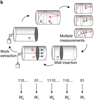
Figure 1: Sketch of the continuous Maxwell demon setup taken from Ref. Ribezzi-Crivellari and Ritort (2019) (Fig. 1b in there).

More specifically, we consider the setup shown in Fig. 1. Initially, the particle is in equilibrium occupying with probability $\pi_{0}=V_{0}/V$ ($\pi_{1}=V_{1}/V$) the volume $V_{0}$ ($V_{1}$). Then, we perform a first measurement of the compartment and repeat the measurement until we see a change of the compartment. Accordingly, we can classify the sequence of measurement results into 0- and 1-cycles denoted by

$$0_{\ell}=(\underbrace{0,\dots,0}_{\ell},1),~{}~{}~{}1_{\ell}=(\underbrace{1,\dots,1}_{\ell},0),$$ (53)

where $\ell\geq 1$ denotes the number of measurements before we measured a change of the compartment. If we have a 0-cycle (1-cycle), we extract an amount of work $W_{1}$ ($W_{0}$) from the system such that the extracted work is on average

$$W^{\text{ext}}=-T(\pi_{0}\ln\pi_{1}+\pi_{1}\ln\pi_{0}).$$ (54)

Interestingly Ribezzi-Crivellari and Ritort (2019), the standard Landauer limit gives a lower instead of an upper bound on the extractable work: $W^{\text{ext}}\geq TS_{\text{Sh}}[\{\pi_{0},\pi_{1}\}]$. The resolution to this ‘paradox’ is, of course, that we have to evaluate the information content of the memory with respect to the cycles of Eq. (53). In the rest of this section we are going to demonstrate that this follows automatically from our general framework.

For this purpose we label by $x\in\{0,1\}$ the mesostates to find the particle in volume $V_{0}$ or $V_{1}$. Importantly, we have to associate an intrinsic entropy to these states given by (remember that $k_{B}\equiv 1$)

$$s_{0}=\ln V_{0}/V,~{}~{}~{}s_{1}=\ln V_{1}/V.$$ (55)

They are computed by assuming that the single particle behaves like an ideal gas such that we can use $Tds=pdV$ with the pressure $p=T/V$. Furthermore, we set the entropy for the state where the particle can occupy the entire volume $V$ for convenience and without loss of generality to zero. Then, the extractable work reads $W_{i}=-Ts_{i}$ provided that the last measurement outcome is $i$. Obviously, the sequence of measurement results $\textbf{r}_{\ell+1}$ is given by the cycles (53) with each $r_{k}\in\{i\}=\{0,1\}$. As in Ref. Ribezzi-Crivellari and Ritort (2019) we now assume perfect measurements such that $S_{\text{Sh}}(\textbf{q})=0$ where q denotes the initial state of the ancilla (or memory) used to record the measurement result. Furthermore, we do not perform any work on the system by changing some protocol $\lambda_{t}$, thus $W^{\text{tot}}=0$. Note that here we equate the final extracted work $W^{\text{ext}}$ with the final change in nonequilibrium free energy when we return the system to its initial state. Therefore, $W^{\text{ext}}$ does not appear in the expression of $W^{\text{tot}}$. Our generalized second law (49) reduces in this case to

$$\begin{split}\Sigma^{\text{tot}}&=S_{\text{Sh}}\left[\{P(\textbf{r}_{n})\}_{\textbf{r}_{n}}\right]\\ &\phantom{==}-\beta\left\{\sum_{\textbf{r}_{n}}P(\textbf{r}_{n})F[\textbf{p}(t_{n}^{+},\textbf{r}_{n})]-F[\textbf{p}(t_{0})]\right\}\geq 0.\end{split}$$ (56)

Here, $n$ is a sufficiently large natural number in the following sense: In each run of the experiment, we will observe a change of the compartment at a different time $\ell\tau$, $\ell\in\mathbb{N}$. After that time we extract the work and restart the experiment. Now, we choose $n$ large enough such that it is almost certain that the particle has changed the compartment by the time $n\tau$, i.e., $P(0_{n})\approx P(1_{n})\approx 0$. The measurement sequences $\textbf{r}_{n}$, e.g. in case of a 0-cycle if the particle has changed compartment at $\ell\tau$, is then written as

$$\textbf{r}_{n}(0_{\ell})=(\underbrace{0,\dots,0}_{\ell},1,\underbrace{0,\dots,0}_{n-\ell-1}),$$ (57)

where we have simply ‘filled in’ zeros for the missing measurement results after we have aborted the experiment. This does not change the probability, i.e. $P[\textbf{r}_{n}(0_{\ell})]=P(0_{\ell})$. To complete the analysis, we take into account that the energy of the particle does not depend on which volume it occupies such that we will conveniently set $e_{x}=0$. Then, if we start in equilibrium as in Ref. Ribezzi-Crivellari and Ritort (2019), the initial free energy becomes

$$F[\textbf{p}(t_{0})]=-T\sum_{x}\pi_{x}(-\ln\pi_{x}+s_{x})=0$$ (58)

since $s_{x}=\ln V_{x}/V=\ln\pi_{x}$. On the other hand, the final free energy reads $-T\ln s_{1}$ ($-T\ln s_{0}$) in case of a 0-cycle (1-cycle) and appears with probability $\pi_{0}$ ($\pi_{1}$). Hence, our second law takes on the simple form

$$\begin{split}\Sigma^{\text{tot}}&=S_{\text{Sh}}\left[\{P(\textbf{r}_{n})\}_{\textbf{r}_{n}}\right]+(\pi_{0}\ln\pi_{1}+\pi_{1}\ln\pi_{0})\\ &=S_{\text{Sh}}\left[\{P(\textbf{r}_{n})\}_{\textbf{r}_{n}}\right]-\beta W^{\text{ext}}\geq 0.\end{split}$$ (59)

In the final step we have used that the extractable work $W^{\text{ext}}$ is precisely given by the change of free energy by letting the particle expand and thereby the system returns to its initial equilibrium configuration.

Thus, our framework immediately leads to the desired result without the need to explicitly compute $S_{\text{Sh}}\left[\{P(\textbf{r}_{n})\}_{\textbf{r}_{n}}\right]$, which was done in Ref. Ribezzi-Crivellari and Ritort (2019) in order to confirm the second law. Remarkably, the above abstract experiment was realized using single molecule pulling experiments finding very good agreement with theory Ribezzi-Crivellari and Ritort (2019).

IV.4 Fluctuation theorems

In this paper we have so far focused on definitions for key thermodynamic quantities along a single stochastic trajectory, but not yet on fluctuation theorems, which are a milestone in nonequilibrium statistical physics Jarzynski (2011); Seifert (2012); Van den Broeck and Esposito (2015). Here, we limit ourselves to a few observations about fluctuations in our framework.

First, the derivation of fluctuation theorems relies on a perfectly observed system state and the microreservibility of the underlying Hamiltonian dynamics of the system and the heat bath. For the causal model considered here, which can deal with any amount of uncertainty and explicitly allows to include (subjective, observer-dependent) control operations in the description, there is no hope of deducing a physically meaningful fluctuation theorem in general – at least none which only depends on the information available in the measurement record $\textbf{r}_{n}$. Note that fluctuation theorems, as typically derived in the presence of feedback control Parrondo et al. (2015), still rely on the ability to perfectly measure the system, compare also with the discussion in Ref. Wächtler et al. (2016).

Second, there always exists a ‘formal’ fluctuation theorem, which we can derive by defining a suitable ‘backward’ or ‘time-reversed’ process. For this purpose, let $\textbf{r}_{n}^{\dagger}$ denote the sequence of measurement results $\textbf{r}_{n}$ in reverse order and let $Q(\textbf{r}_{n}^{\dagger})$ be the probability to observe this sequence in the backward experiment, typically carried out by reversing the driving protocol $\lambda_{t}$. Then, given that $Q(\textbf{r}_{n}^{\dagger})=0$ only if $P(\textbf{r}_{n})=0$, we always have the trivial fluctuation theorem

$${\left\langle{e^{-\tilde{\Sigma}(\textbf{r}_{n})}}\right\rangle}_{\textbf{r}_{n}}\equiv\sum_{\textbf{r}_{n}}P(\textbf{r}_{n})e^{-\tilde{\Sigma}(\textbf{r}_{n})}=1,$$ (60)

if we define the ‘entropy production’

$$\tilde{\Sigma}(\textbf{r}_{n})\equiv\ln\frac{P(\textbf{r}_{n})}{Q(\textbf{r}_{n}^{\dagger})}.$$ (61)

While this quantity measures some asymmetry of the measurement statistics under time-reversal, there is no obvious connection of it to any thermodynamic quantity introduced above. Thus, outside the traditional limit of stochastic thermodynamics, Eq. (60) lacks any relation to a meaningful physical quantity and therefore, does not share the same status as the conventional fluctuation theorem Jarzynski (2011); Seifert (2012); Van den Broeck and Esposito (2015).

Obviously, in the limit of a perfect and continuous bare measurement, our definitions allow to sample, e.g., the exact microscopic work statistics and derivations of fluctuation theorems become possible again. Remarkably, even outside this limit we can derive a general inequality, which links the observed work statistics to the Jarzynski equality Jarzynski (1997a, b). Let us write the observed Jarzynski equality as

$${\left\langle{e^{-\beta W(\textbf{r}_{n})}}\right\rangle}_{\textbf{r}_{n}}\equiv e^{-\beta\Delta F_{\text{est}}},$$ (62)

where $\Delta F_{\text{est}}$ denotes the estimated free energy difference based on the available work statistics. Furthermore, let us denote by $\boldsymbol{\gamma}$ a system trajectory obtained from a perfect continuous measurement such that Jarzynski (1997a, b)

$${\left\langle{e^{-\beta W(\boldsymbol{\gamma})}}\right\rangle}_{\boldsymbol{\gamma}}=e^{-\beta\Delta F}.$$ (63)

Finally, we introduce the conditional probability $P(\boldsymbol{\gamma}|\textbf{r}_{n})$ that the microscopic trajectory was $\boldsymbol{\gamma}$ given that we obtained the measurement record $\textbf{r}_{n}$. Now, for bare measurements we can always view the observed work $W(\textbf{r}_{n})$ as resulting from a coarse-grained measurement of the perfectly measured work $W(\boldsymbol{\gamma})$, i.e.

$$W(\textbf{r}_{n})=\sum_{\boldsymbol{\gamma}}W(\boldsymbol{\gamma})P(\boldsymbol{\gamma}|\textbf{r}_{n}).$$ (64)

Since the exponential function is convex, we immediately obtain, by Jensen’s inequality,

$${\left\langle{e^{-\beta W(\textbf{r}_{n})}}\right\rangle}_{\textbf{r}_{n}}\leq{\left\langle{e^{-\beta W(\boldsymbol{\gamma})}}\right\rangle}_{\boldsymbol{\gamma}},$$ (65)

or, equivalently for the free energy differences,

$$\Delta F_{\text{est}}\geq\Delta F.$$ (66)

Hence, as any experiment involves measurement errors and since the exponential function is actually strictly convex, we can conclude that the estimated free energy difference in any Jarzynski-type experiment always overestimates the actual free energy difference: $\Delta F_{\text{est}}>\Delta F$. Particular estimates for the difference $\Delta F_{\text{est}}-\Delta F$ are hard to compute in general, but were worked out for particular models in Refs. García-García et al. (2016); Wächtler et al. (2016).

IV.5 Comparison with the framework
of Ito & Sagawa

Stochastic thermodynamics of a causal model was already studied by Ito and Sagawa for so-called Bayesian networks Ito and Sagawa (2013, 2016). For an early study in that direction connecting information theory, entropy and causal models on an average level see also Ref. Touchette and Lloyd (2004). Here we will outline how to connect our description to a Bayesian network and we will briefly highlight a few key differences in the thermodynamic description. A thorough comparison, however, is beyond the scope of the present paper, as in its most general form both frameworks, the present one and the one of Refs. Ito and Sagawa (2013, 2016), are quite involved.

Bayesian networks are a graphical representation of a probabilistic model, in which all random variables are specified by the nodes of the network and the conditional dependencies are represented by directed edges. Mathematically, a Bayesian network is thus given by a directed acyclic graph, which reflects the causal structure of the problem. Physically speaking, a directed acyclic graph corresponds to the fact that time ‘flows’ in one direction and no time-loops are possible. The Bayesian network is fully specified once the probability distribution of the input variables and the conditional probabilities for all edges are known.

Figure 2: Bayesian network associated to a process with two control operations.

For illustration, we depict the Bayesian network for two control operations in Fig. 2. It basically consists of three ‘layers’. The first layer describes the evolution of the system $X$, where we used $x_{i}^{\pm}$ to denote the state of the system at time $t_{i}^{\pm}$. To construct the control operations at time $t_{i}$, we use a second layer of auxiliary systems $Y_{i}$ with states $y_{i}^{\pm}$ (the ancillas). The final layer of observations by the external agent is described by the measurement results $r_{i}$. Based on these measurement results, the external agent can decide to change the system evolution controlled by the protocol $\lambda_{t}$ or to change the next control operation, or both. For simplicity, we depicted only two control operations in Fig. 2 because the density of arrows in the picture quickly becomes very large as all previous results are allowed to influence the future evolution and control operations. Thus, our framework can be formulated in terms of a Bayesian network and could be analysed using the tools of Refs. Ito and Sagawa (2013, 2016), but there are also some essential differences in our setting and thermodynamic analysis.

First, Ito and Sagawa assume that the control protocol $\lambda_{t}$ is constant in between two control operations and changes only in a step-wise fashion at the times $t_{i}$. This seems to be an essential element in their formulation in order to derive the second law based on the concept of a ‘backward trajectory’, where transitions in the system state are required to be linked to entropy exchanges in the bath. Within our formalism we see that there is no need to assume that $\lambda_{t}$ remains fixed in between two control operations. Moreover, Ito and Sagawa assume that any change in energy due to a transition in the system state is due to an entropy change in the bath, see for instance Eq. (4) in Ref. Ito and Sagawa (2013). This, however, implies that they exclude the possibility of any deterministic changes in the state of the system due to an external control operation. In other words, the work invested in the control operation is always zero in their case, $W^{\text{ctrl}}(t_{n},\textbf{r}_{n-1})=0$, and hence it seems reasonable to compare their framework with the ‘bare measurement’ case of our framework.

Also their thermodynamic conclusions are slightly different from ours. Apart from the already mentioned missing work contribution during the control step, our second laws are different, too. Instead of the change in entropy in the external stream of ancillas and the measurement record [cf. Eq. (49)], their second law contains the transfer entropy from the first layer (the system) to the second and third layer. The transfer entropy is an asymmetric, directed generalization of the mutual information concept Schreiber (2000), and therefore the second law derived in Refs. Ito and Sagawa (2013, 2016) is closer in spirit to the second law of Ref. Parrondo et al. (2015). In our language, their second law corresponds to the case of an ‘uninformed’ agent as discussed at the end of the previous section.

V Final remarks

We have provided definitions for stochastic internal energy, heat, work and entropy, which can be computed by an external observer who can manipulate a small system with arbitrary instantaneous interventions and who has no access to any further information. While the definition of internal energy remained the same as usual, the non-trivial effect of the external interventions forced us to associate a novel notion of work [Eq. (26)] and heat [Eq. (27)] to it. Mathematically, we achieved this by using a classical version of Stinespring’s dilation theorem (Theorem II.1), and we ensured that we reproduce previous notions for already well-studied limiting cases. Hence, the first law at the trajectory level takes on the same form as usual and can reproduce the standard case of stochastic thermodynamics for a perfectly and continuously measured system Strasberg (2018).

In contrast to the internal energy, we had to redefine the notion of system entropy from the start [Eq. (31)]. Following the motto “information is physical” Landauer (1991), we explicitly included the information generated by the measurements. We then showed that the stochastic entropy production – defined in the standard way as the change in (redefined) system entropy plus the change in entropy of the bath (which is proportional to the heat flow from it) – is positive on average for any set of external interventions. While we do not reproduce the standard notion of stochastic entropy Seifert (2005, 2012); Van den Broeck and Esposito (2015) in the respective limit, our choice guarantees that there is no need to modify the second law in the presence of feedback control.

To summarize, the present paper puts forward a formally consistent framework of stochastic thermodynamics for an arbitrarily controlled system in contact with a single heat bath. Our causal model relies solely on the approximation that the external interventions are happening instantaneously. The very general, but also abstract framework of Section III allows us to draw three conclusions. First, the second law in presence of feedback control is more naturally expressed in terms of the Shannon entropy of the memory than the mutual information between the system and the memory. Second, our definition of stochastic entropy suggests that the stochastic entropy of Ref. Seifert (2005) actually measures the entropy of the memory and not the system. Third, on a very abstract level, it appears that this framework is very similar to its quantum counterpart Strasberg (2018), demonstrating that thermodynamics is a universal theory where similar principles apply to both, classical and quantum systems alike. In addition, we have also shown in Section IV that our theory allows to draw practically relevant conclusions.

For the future we connect the hope with our framework that it lays the foundation to study problems of thermodynamic inference, such as those in Refs. Ribezzi-Crivellari and Ritort (2014); Alemany et al. (2015); Polettini and Esposito (2017, 2019), within one common unified framework. In that respect it would be very important to extend the present theory to multiple heat reservoirs too Polettini and Esposito (2017, 2019). In addition, for practical applications it would be desirable to gain further insights into the physical nature of the rather abstract ancillas introduced by us.

Acknowledgments

We are grateful for the useful comments of the two anonymous referees. The authors were partially supported by the Spanish MINECO (project FIS2016-86681-P) with the support of FEDER funds, and the Generalitat de Catalunya (project 2017-SGR-1127). PS is financially supported by the DFG (project STR 1505/2-1).

Appendix A Proof of the classical
Stinespring representation Theorem II.1

Our proof will be constructive and we start with the representation provided in Eq. (11). For this purpose we use the fact (see Ref. Ye et al. (2016)) that every stochastic matrix $A$ can be decomposed as

$$A=\sum_{\xi=1}^{N}\lambda_{\xi}F^{(\xi)},$$ (67)

with $N\leq d^{2}-d+1$. Here, the $\lambda_{\xi}$ are probabilities (i.e. $\lambda_{\xi}\geq 0$ and $\sum_{\xi}\lambda_{\xi}=1$) and $F^{(\xi)}$ are deterministic transition matrices. This means they are binary, $F^{(\xi)}_{x,x^{\prime}}\in\{0,1\}$, and they have exactly one ‘1’ in each column, otherwise all entries are $0$. In general, $F^{(\xi)}$ is not invertible, but the set of invertible deterministic transition matrices coincides with the set of permutation matrices. Furthermore, we remark that the decomposition (67) is in general not unique.

To prove Eq. (11), we notice that the matrix elements of every deterministic transition matrix can be expressed as $F^{(\xi)}_{x,x^{\prime}}=\delta_{x,f_{\xi}(x^{\prime})}$ where $f_{\xi}:X\rightarrow X$ is a function on the state space $X=\{1,\dots,d\}$ of the system, mapping $x^{\prime}\in X$ to $x=f_{\xi}(x^{\prime})\in X$, and $\delta_{x,x^{\prime}}$ denotes the Kronecker delta. We now need to extend the set of functions $\{f_{\xi}\}$ to a single function, which is invertible and defined on a larger space $X\times Y$ where $Y$ denotes the state space of the ancilla. A construction that achieves this is given by $Y=Z\times\Xi$, where $Z=\{1,\dots,d\}$ can be regarded as a register to copy the state of $X$, and $\Xi=\{1,\dots,d^{2}-d+1\}$ labels the different functions used in Eq. (67). Then, we define

$$\Pi:X\times Z\times\Xi\ni(x,z,\xi)\mapsto(f_{\xi}(x)+z-1,x,\xi)\in X\times Z\times\Xi,$$ (68)

where the summation in the first register is understood modulo $d$. This function is clearly invertible, hence it is a permutation: Namely, given $x$ and $\xi$, which are copied into the second and third register, we know $f_{\xi}(x)$ and from that we obtain $z$ from the first register. Hence, we can associate a permutation matrix $\Pi$ to it, which has elements

$$\Pi_{xz\xi,x^{\prime}z^{\prime}\xi^{\prime}}=\delta_{x,f_{\xi^{\prime}}(x^{\prime})+z^{\prime}-1}\delta_{z,x^{\prime}}\delta_{\xi,\xi^{\prime}}.$$ (69)

Finally, we choose the initial state of the environment to be $q_{z\xi}=\delta_{z,1}\lambda_{\xi}$, which gives

$$\sum_{z,\xi,z^{\prime},\xi^{\prime}}\Pi_{xz\xi,x^{\prime}z^{\prime}\xi^{\prime}}q_{z^{\prime}\xi^{\prime}}=\sum_{\xi}\delta_{x,f_{\xi}(x^{\prime})}\lambda_{\xi}=\sum_{\xi}F_{x,x^{\prime}}^{(\xi)}\lambda_{\xi},$$ (70)

as desired.

Next, to prove Eq. (12), we first of all note that any stochastic matrix $A$ can be decomposed into at most $d^{2}$ many different independent control operations $A(r)$ such that $A=\sum_{r}A(r)$. Any further control operation must then be a linear combination of the previous operations and as any representation of a causal model is linear in the applied operations $A(r)$ Pollock et al. (2018b); Milz et al. (2017), it suffices to consider $d^{2}$ independent ones. Thus, we choose $r$ to have two components, labeled $r=(\bar{x},\bar{x}^{\prime})$, and consider the elementary control operations $A(\bar{x},\bar{x}^{\prime})$ with elements

$$A_{x,x^{\prime}}(\bar{x},\bar{x}^{\prime})=\delta_{x,\bar{x}}\delta_{x^{\prime},\bar{x}^{\prime}}A_{x,x^{\prime}}.$$ (71)

Any other decomposition of $A$ into different control operations $\tilde{A}(r)$ can be obtained from the above decomposition via linear combination, i.e. $\tilde{A}(r)=\sum_{\bar{x},\bar{x}^{\prime}}\mu_{\bar{x},\bar{x}^{\prime}}(r)A(\bar{x},\bar{x}^{\prime})$, for some set of positive coefficients $\{\mu_{\bar{x},\bar{x}^{\prime}}(r)\}$ which satisfy $\sum_{r}\mu_{\bar{x},\bar{x}^{\prime}}(r)=1$ for all $(\bar{x},\bar{x}^{\prime})$.

Now we construct the bare measurement matrix $B_{y,y^{\prime}}(\bar{x},\bar{x}^{\prime})$ for the elementary decomposition considered above. For this purpose, we introduce the subsets

$$\Xi_{x,x^{\prime}}=\{\xi\in\Xi|f_{\xi}(x^{\prime})=x\}\subset\Xi.$$ (72)

These sets collect all $\xi\in\Xi$ which map a chosen $x^{\prime}$ to a chosen $x$. We then define the diagonal matrix $B(r)$ via

$$B_{z\xi,z\xi}(\bar{x},\bar{x}^{\prime})\equiv\sum_{\bar{\xi}\in\Xi_{\bar{x},\bar{x}^{\prime}}}\delta_{z,\bar{x}^{\prime}}\delta_{\xi,\bar{\xi}}.$$ (73)

Using the constructions for the permutation matrix $\Pi$ and the probability vector q from above, we confirm that

$$\sum_{y,y^{\prime}}B_{y,y}(\bar{x},\bar{x}^{\prime})\Pi_{xy,x^{\prime}y^{\prime}}q_{z^{\prime}\xi^{\prime}}=\sum_{\bar{\xi}\in\Xi_{\bar{x},\bar{x}^{\prime}}}\delta_{x^{\prime},\bar{x}^{\prime}}\delta_{x,f_{\bar{\xi}}(\bar{x}^{\prime})}\lambda_{\bar{\xi}}.$$ (74)

On the other hand, by the definition of $A(r)$ in Eq. (71) and the decomposition (67), we have

$$\begin{split}A_{x,x^{\prime}}(\bar{x},\bar{x}^{\prime})&=\delta_{x,\bar{x}}\delta_{x^{\prime},\bar{x}^{\prime}}\sum_{\xi}\delta_{x,f_{\xi}(x^{\prime})}\lambda_{\xi}\\ &=\sum_{\bar{\xi}\in\Xi_{\bar{x},\bar{x}^{\prime}}}\delta_{x,\bar{x}}\delta_{x^{\prime},\bar{x}^{\prime}}\delta_{x,f_{\bar{\xi}}(\bar{x}^{\prime})}\lambda_{\bar{\xi}}.\end{split}$$ (75)

Apart from the factor $\delta_{x,\bar{x}}$ this is identical to Eq. (74). But this factor is actually redundant: once we know the input $x^{\prime}=\bar{x}^{\prime}$, the output $x$ is fixed because the sum is restricted to only those functions which map a given input $\bar{x}^{\prime}$ to a given output $\bar{x}$. Hence, we have proven Eq. (12). ∎

While the above construction is quite convenient, we emphasize that it is not necessarily optimal, in the sense that in general it will be possible to find a representation with an ancilla space of dimension $D<d(d^{2}-d+1)$. In fact, all what we need to ensure when constructing the permutation matrix $\Pi$ is that, for any given output state $x\in X$ and any fixed decomposition (67) into $N\leq d^{2}-d+1$ deterministic transition matrices, the ancilla space $Y$ has enough states to label which actual state $x^{\prime}\in X$ was mapped to $x=f_{\xi}(x^{\prime})$ for every possible $\xi\in\{1,\dots,N\}$. This would then allow us to construct an injection $F:X\times\{1,\dots,N\}\hookrightarrow X\times Y$, which we could extend to a bijection and represent by a permutation matrix $\Pi$. Let us denote by $|f^{-1}_{\xi}(x)|$ the number of elements in the preimage of $x$ under $f_{\xi}$. Then, the state space $Y$ must have dimension

$$D=\max_{x}\sum_{\xi}|f^{-1}_{\xi}(x)|,$$ (76)

which fulfills $Nd>D\geq N$. The latter inequality implies that the state space $Y$ must have, for a fixed decomposition (67), at least $N$ elements. To see this, consider the table of cardinalities $M_{\xi,x}\equiv|f_{\xi}^{-1}(x)|$. Because every $f_{\xi}$ is a function, every row of $M_{\xi,x}$ must sum up to $d$. This means that $Dd\geq\sum_{x}\sum_{\xi}M_{\xi,x}=\sum_{\xi}d=Nd$, hence $D\geq N$. On the other hand, the worst case scenario for a single function $\xi$ is that $|f_{\xi}^{-1}(x)|=d$, i.e. all input states get mapped to the same ouput state $x$. Then, $D=Nd$ implies that all functions $\xi$ map all states to the same $x$. But then the decomposition (67) is actually redundant as all functions $\xi$ were identical. Hence, we can always choose $D<Nd=d(d^{2}-d+1)$ implying that our construction above is not optimal.

Finally, we have to keep in mind that the decomposition (67) is not unique. Hence, the minimum dimension $D_{\text{min}}$ of the ancilla space is obtained by minimizing over all possible decompositions, i.e.

$$D_{\text{min}}=\min_{\{\xi\}}\max_{x}\sum_{\xi}|f^{-1}_{\xi}(x)|.$$ (77)

Let us exemplify this reasoning in the simplest possible case of $A$ being a $2\times 2$ matrix, i.e. it describes a 1-bit channel. There are exactly four deterministic transition matrices: the identity, the bit-flip operation and the two matrices which map any input either to ‘0’ or to ‘1’, respectively. Any possible $A$ can then be written as a convex combination of the invertible identity map, the invertible bit-flip and one (but only one) of the two other non-invertible maps. For the invertible maps we obviously have $|f^{-1}_{\xi}(x)|=1$ for every $x$ and for any of the non-invertible maps we have $\max_{x}|f^{-1}_{\xi}(x)|=2$. Thus, we need at most $D=d^{2}=4$ ancilla states for the case of the 1-bit channel, whereas our explicit construction above suggested that $D=d(d^{2}-d+1)=6$ is needed. Unfortunately, evaluating Eq. (77) for higher dimensions becomes hard very quickly.

References

- Bustamante et al. (2005) C. Bustamante, J. Liphardt, and F. Ritort, “The nonequilibrium thermodynamics of small systems,” Phys. Today 58, 43–48 (2005).
- Sekimoto (2010) K. Sekimoto, Stochastic Energetics, Vol. 799 (Lect. Notes Phys., Springer, Berlin Heidelberg, 2010).
- Jarzynski (2011) C. Jarzynski, “Equalities and inequalities: irreversibility and the second law of thermodynamics at the nanoscale,” Annu. Rev. Condens. Matter Phys. 2, 329–351 (2011).
- Seifert (2012) U. Seifert, “Stochastic thermodynamics, fluctuation theorems and molecular machines,” Rep. Prog. Phys. 75, 126001 (2012).
- Van den Broeck and Esposito (2015) C. Van den Broeck and M. Esposito, “Ensemble and trajectory thermodynamics: A brief introduction,” Physica (Amsterdam) 418A, 6–16 (2015).
- Ciliberto (2017) S. Ciliberto, “Experiments in stochastic thermodynamics: Short history and perspectives,” Phys. Rev. X 7, 021051 (2017).
- Ribezzi-Crivellari and Ritort (2014) M. Ribezzi-Crivellari and F. Ritort, “Free-energy inference from partial work measurements in small systems,” Proc. Natl. Acad. Sci. 111, 3386–3394 (2014).
- Alemany et al. (2015) A. Alemany, M. Ribezzi-Crivellari, and F. Ritort, “From free energy measurements to thermodynamic inference in nonequilibrium small systems,” New. J. Phys. 17, 075009 (2015).
- Bechhoefer (2015) J. Bechhoefer, “Hidden Markov models for stochastic thermodynamics,” New. J. Phys. 17, 075003 (2015).
- García-García et al. (2016) R. García-García, L. Sourabh, and D. Lacoste, “Thermodynamic inference based on coarse-grained data or noisy measurements,” Phys. Rev. E 93, 032103 (2016).
- Wächtler et al. (2016) C. W. Wächtler, P. Strasberg, and T. Brandes, “Stochastic thermodynamics based on incomplete information: generalized Jarzynski equality with measurement errors with or without feedback,” New J. Phys. 18, 113042 (2016).
- Polettini and Esposito (2017) M. Polettini and M. Esposito, “Effective thermodynamics for a marginal observer,” Phys. Rev. Lett. 119, 240601 (2017).
- Polettini and Esposito (2019) M. Polettini and M. Esposito, “Effective fluctuation and response theory,” J. Stat. Phys. (2019).
- Parrondo et al. (2015) J. M. R. Parrondo, J. M. Horowitz, and T. Sagawa, “Thermodynamics of information,” Nat. Phys. 11, 131–139 (2015).
- Wolpert (2019) D. Wolpert, “The stochastic thermodynamics of computation,” J. Phys. A: Math. Theor. 52, 193001 (2019).
- Strasberg (2018) P. Strasberg, “An operational approach to quantum stochastic thermodynamics,” arXiv 1810.00698 (2018).
- Pearl (2009) J. Pearl, Causality: Models, Reasoning and Inference (Cambridge University Press, 2009).
- Ito and Sagawa (2013) S. Ito and T. Sagawa, “Information thermodynamics on causal networks,” Phys. Rev. Lett. 111, 180603 (2013).
- Ito and Sagawa (2016) S. Ito and T. Sagawa, Mathematical Foundations and Applications of Graph Entrop, edited by M. Dehmer, F. Emmert-Streib, Z. Chen, and Y. Shi (Wiley-VCH Verlag, Weinheim, 2016) Title: Information flow and entropy production on Bayesian networks.
- Liphardt et al. (2002) J. Liphardt, S. Dumont, S. B. Smith, I. Tinoco, and C. Bustamante, “Equilibrium information from nonequilibrium measurements in an experimental test of Jarzynski’s equality,” Science 296, 1832–1835 (2002).
- Douarche et al. (2005) F. Douarche, S. Ciliberto, A. Petrosyan, and I. Rabbiosi, “An experimental test of the Jarzynski equality in a mechanical experiment,” Europhys. Lett. 70, 593 (2005).
- Gupta et al. (2011) A. N. Gupta, A. Vincent, K. Neupane, H. Yu, F. Wang, and M. T. Woodside, “Experimental validation of free-energy-landscape reconstruction from non-equilibrium single-molecule force spectroscopy measurements,” Nat. Phys. 7, 631 (2011).
- Raman et al. (2014) S. Raman, T. Utzig, B. Ratna Shrestha T. Baimpos, and M. Valtiner, “Deciphering the scaling of single-molecule interactions using Jarzynski’s equality,” Nat. Comm. 5, 5539 (2014).
- Ribezzi-Crivellari and Ritort (2019) M. Ribezzi-Crivellari and F. Ritort, “Large work extraction and the Landauer limit in a continuous Maxwell demon,” Nat. Phys. 15, 660 – 664 (2019).
- Wiseman and Milburn (2010) H. M. Wiseman and G. J. Milburn, Quantum Measurement and Control (Cambridge University Press, Cambridge, 2010).
- Pollock et al. (2018a) F. A. Pollock, C. Rodríguez-Rosario, T. Frauenheim, M. Paternostro, and K. Modi, “Operational Markov condition for quantum processes,” Phys. Rev. Lett. 120, 040405 (2018a).
- Pollock et al. (2018b) F. A. Pollock, C. Rodríguez-Rosario, T. Frauenheim, M. Paternostro, and K. Modi, “Non-Markovian quantum processes: Complete framework and efficient characterization,” Phys. Rev. A 97, 012127 (2018b).
- Milz et al. (2017) S. Milz, F. Sakuldee, F. A. Pollock, and K. Modi, “Kolmogorov extension theorem for (quantum) causal modelling and general probabilistic theories,” arXiv: 1712.02589 (2017).
- Stinespring (1955) W. F. Stinespring, “Positive functions on -algebras,” Proc. Am. Math. Soc. 6, 211–216 (1955).
- Seifert (2011) U. Seifert, “Stochastic thermodynamics of single enzymes and molecular motors,” Eur. Phys. J. E 34, 26 (2011).
- Esposito (2012) M. Esposito, “Stochastic thermodynamics under coarse graining,” Phys. Rev. E 85, 041125 (2012).
- Strasberg and Esposito (2019) P. Strasberg and M. Esposito, “Non-Markovianity and negative entropy production rates,” Phys. Rev. E 99, 012120 (2019).
- Strasberg (2019) P. Strasberg, “Repeated interactions and quantum stochastic thermodynamics at strong coupling,” arXiv: 1907.01804 (2019).
- Strasberg et al. (2017) P. Strasberg, G. Schaller, T. Brandes, and M. Esposito, “Quantum and information thermodynamics: A unifying framework based on repeated interactions,” Phys. Rev. X 7, 021003 (2017).
- Elouard et al. (2017) C. Elouard, D. A. Herrera-Martií, M. Clusel, and A. Auffèves, “The role of quantum measurement in stochastic thermodynamics,” npj Quantum Inf. 3, 9 (2017).
- Seifert (2005) U. Seifert, “Entropy production along a stochastic trajectory and an integral fluctuation theorem,” Phys. Rev. Lett. 95, 040602 (2005).
- Landauer (1991) R. Landauer, “Information is physical,” Phys. Today 44, 23 (1991).
- Boyd et al. (2018) A. B. Boyd, D. Mandal, and J. P. Crutchfield, “Thermodynamics of modularity: Structural costs beyond the Landauer bound,” Phys. Rev. X 8, 031036 (2018).
- Strasberg et al. (2013) P. Strasberg, G. Schaller, T. Brandes, and M. Esposito, “Thermodynamics of quantum-jump-conditioned feedback control,” Phys. Rev. E 88, 062107 (2013).
- Munakata and Rosinberg (2014) T. Munakata and M. L. Rosinberg, “Entropy production and fluctuation theorems for Langevin processes under continuous non-Markovian feedback control,” Phys. Rev. Lett. 112, 180601 (2014).
- Rosinberg et al. (2015) M. L. Rosinberg, T. Munakata, and G. Tarjus, “Stochastic thermodynamics of Langevin systems under time-delayed feedback control: Second-law-like inequalities,” Phys. Rev. E 91, 042114 (2015).
- Xiao (2016) T. Xiao, “Heat dissipation and information flow for delayed bistable Langevin systems near coherence resonance,” Phys. Rev. E 94, 052109 (2016).
- Loos and Klapp (2019) S. A. M. Loos and S. H. L. Klapp, “Heat flow due to time-delayed feedback,” Sci. Rep. 9, 2491 (2019).
- Mandal and Jarzynski (2012) D. Mandal and C. Jarzynski, “Work and information processing in a solvable model of Maxwell’s demon,” Proc. Natl. Acad. Sci. 109, 11641–11645 (2012).
- Deffner and Jarzynski (2013) S. Deffner and C. Jarzynski, “Information processing and the second law of thermodynamics: An inclusive, Hamiltonian approach,” Phys. Rev. X 3, 041003 (2013).
- Schaller et al. (2011) G. Schaller, C. Emary, G. Kiesslich, and T. Brandes, “Probing the power of an electronic Maxwell’s demon: Single-electron transistor monitored by a quantum point contact,” Phys. Rev. B 84, 085418 (2011).
- Averin et al. (2011) D. V. Averin, M. Möttönen, and J. P. Pekola, “Maxwell’s demon based on a single-electron pump,” Phys. Rev. B 84, 245448 (2011).
- Esposito and Schaller (2012) M. Esposito and G. Schaller, “Stochastic thermodynamics for ”Maxwell demon” feedbacks,” Europhys. Lett. 99, 30003 (2012).
- Chida et al. (2017) K. Chida, S. Desai, K. Nishiguchi, and A. Fujiwara, “Power generator driven by Maxwell’s demon,” Nat. Comm. 8, 15310 (2017).
- Jarzynski (1997a) C. Jarzynski, “Nonequilibrium equality for free energy differences,” Phys. Rev. Lett. 78, 2690 (1997a).
- Jarzynski (1997b) C. Jarzynski, “Equilibrium free-energy differences from nonequilibrium measurements: A master-equation approach,” Phys. Rev. E 56, 5018–5035 (1997b).
- Touchette and Lloyd (2004) H. Touchette and S. Lloyd, “Information-theoretic approach to the study of control systems,” Physica A 331, 140–172 (2004).
- Schreiber (2000) T. Schreiber, “Measuring information transfer,” Phys. Rev. Lett. 85, 461–464 (2000).
- Ye et al. (2016) F. X.-F. Ye, Y. Wang, and H. Qian, “Stochastic dynamics: Markov chains and random transformations,” Disc. Contin. Dyn. Syst. B 21, 2337–2361 (2016).