Topological Classification of Excitations in Quadratic Bosonic Systems

Abstract

We investigate the topological classification of excitations in quadratic bosonic systems with an excitation band gap. Time-reversal, charge-conjugation, and parity symmetries in bosonic systems are introduced to realize a ten-fold symmetry classification. We find a specific decomposition of the quadratic bosonic Hamiltonian and use it to prove that each quadratic bosonic system is homotopic to a direct sum of two single-particle subsystems. The topological classification table is thus derived via inheriting from that of Atland-Zirnbauer classes and unique topological phases of bosons are predicted. Finally, concrete topological models are proposed to demonstrate the peculiarity of bosonic excitations.

I Introduction

Searching for topological phases of a many-body system with specific symmetries becomes an important issue in both condensed matter and cold atom physics. As a milestone work, gapped free-fermion systems including the Chern insulator Haldane (1988), topological insulator Kane and Mele (2005a, b); Bernevig et al. (2006); Fu and Kane (2007) and topological superconductor Read and Green (2000); Kitaev (2001); Mourik et al. (2012); Sato and Ando (2017) are categorized into ten symmetry classes according to the time-reversal, charge-conjugation, and chiral symmetries Altland and Zirnbauer (1997); Zirnbauer (2010), which is known as the Atland-Zirnbauer (AZ) classification. The relevant topological phases are classified by a periodic table in the framework of K-theory Stone et al. (2011); Kitaev (2009); Zhao and Wang (2013); Chiu et al. (2016). Recently, the concept of topological phase has also been extended to dynamical Chang (2018); Yang et al. (2018); Gong and Ueda (2018); Qiu et al. (2018) and open quantum-mechanical systems Shen et al. (2018); Kawabata et al. (2018); Yao and Wang (2018); Yao et al. (2018); Kawabata et al. (2019a). The classifications of Floquet topological insulator Roy and Harper (2017) and non-Hermitian systems Gong et al. (2018); Kawabata et al. (2019b) are also established based on similar classification principles.

Parallel to the fermionic insulator, topological phases also emerge from excitations of a bosonic system. They not only are attainable from the simulation of single-particle topological bands Haldane and Raghu (2008); Wang et al. (2008); Chong et al. (2008); Hafezi et al. (2011, 2013); Poo et al. (2011, 2016); Skirlo et al. (2014, 2015); Wang et al. (2009); Aidelsburger et al. (2013, 2014) but also are discovered in peculiar bosonic systems without fermionic analogy. It is reported that the bosonic Bogoliubov-de Gennes (BdG) model containing two-boson annihilation/creation interactions Ring and Schuck (1980); Rossignoli and Kowalski (2005); Blaizot and Ripka (1986) is capable of hosting excitation band with non-vanishing Chern number or $\mathbb{Z}_{2}$ index, which is realizable in magnonic crystals Shindou et al. (2013); Chisnell et al. (2015); Roldán-Molina et al. (2016); Díaz et al. (2019); Kondo et al. (2019, 2019), nonlinear bosonic systems Bardyn et al. (2016), photonic crystals Peano et al. (2016), and ultracold bosonic atoms in optical lattices Engelhardt and Brandes (2015); Xu et al. (2016); Di Liberto et al. (2016); Luo et al. (2018). These bosonic excitation modes are obtained by a pseudo-unitary diagonalization, i.e., Bogoliubov transformation, which keeps the bosonic commutation relation Colpa (1986); Simon et al. (1999). Thus, the topological obstruction, i.e., the energy gap, is defined in an exotic way. Moreover, the stability of bosonic Hamiltonians requires the semi-positive definiteness that brings a limitation on the symmetries. These facts suggest that the symmetry and topology of bosonic systems are qualitatively different from those in the fermionic cases. Therefore, the bosonic excitations are expected to generate peculiar topological phases beyond the common AZ classification.

Then a problem naturally arises: It remains unclear if the topological phases of bosonic excitation exist in other dimensions and symmetry classes. Hence it is of great necessity to achieve their symmetry and topological classifications.

In this paper, we focus on excitations of a quadratic bosonic system (QBS) with an excitation band gap and systematically classify their topological phases according to symmetries. We firstly inherit the AZ classification scheme to introduce the time reversal, charge conjugation, and their composite interpreted as parity and generate a ten-fold symmetry classification for the QBS. We then explore the topological structure of the bosonic Hamiltonian via a specific decomposition which reveals that each QBS is homotopic to a direct sum of two single-particle subsystems. Therefore, the classification table is derived via the periodic table of AZ classes. We further apply these results to predict unique topological phases of bosons and construct concrete bosonic models without fermionic single-particle counterpart. Our work opens a route to explore the topological phases and effects of bosons.

The paper is organized as follows: In Sec. II, we put forward the model of QBS and give the symmetry classification. The decomposition of bosonic Hamiltonian is derived. In Sec. III, the topological classification of excitations in QBS is made and the topological invariants are discussed. In Sec. IV, concrete examples of interaction-driven topological phases are constructed. In Sec. V, conclusions are made.

II Quadratic bosonic system

II.1 Model

We consider a quadratic Hamiltonian $\mathcal{H}=\sum_{k}\phi^{\dagger}\left(k\right)H\left(k\right)\phi\left(k\right)$ composed by bosonic field operators $\phi^{\dagger}\left(k\right)=\left(\begin{array}[]{cc}\boldsymbol{a}^{\dagger}\left(k\right)&\boldsymbol{b}\left(-k\right)\end{array}\right)$ and an Hermitian matrix $H\left(k\right)$ which is continuous with regard to wave vector $k$. Here, $\boldsymbol{a}^{\dagger}=\left(\begin{array}[]{ccc}a_{1}^{\dagger}&\cdots&a_{N}^{\dagger}\end{array}\right)$ and $\boldsymbol{b}=\left(\begin{array}[]{ccc}b_{1}&\cdots&b_{N^{\prime}}\end{array}\right)$ are bosonic creation and annihilation operators, respectively. The field operators obey bosonic commutation relations

$$\left[\phi_{i}\left(k\right),\phi_{j}^{\dagger}\left(k\right)\right]=\tau_{ij},\leavevmode\nobreak\ \tau=\left(\begin{array}[]{cc}\mathbb{I}_{N}\\ &-\mathbb{I}_{N^{\prime}}\end{array}\right),$$ (1)

where $\mathbb{I}_{N}$ denotes $N\times N$ identity matrix. To stabilize the system, $H\left(k\right)$ is required to be semi-positive definite. This general QBS has included the single-particle system ($\boldsymbol{b}\left(k\right)$ vanishing) Wang et al. (2008); Skirlo et al. (2014, 2015); Aidelsburger et al. (2013, 2014); Yan and Zhou (2018) and the widely studied bosonic BdG system ($b_{i}\left(k\right)=a_{i}\left(k\right)$, $N=N^{\prime}$) Shindou et al. (2013); Bardyn et al. (2016); Peano et al. (2016); Engelhardt and Brandes (2015); Xu et al. (2016); Di Liberto et al. (2016); Luo et al. (2018).

We aim to investigate the excitation bands on top of a bosonic ground state, which are solved via a linear transformation $\phi\left(k\right)=V\left(k\right)\psi\left(k\right)$. To satisfy the bosonic commutation relation Eq. (1), the transformation matrix needs to obey $V^{\dagger}\tau V=\tau$ and forms a pseudo-unitary group $U\left(N,N^{\prime}\right)$. As a mathematical theorem Simon et al. (1999), each positive definite Hermitian matrix $H$ is pseudo-unitarily congruent to a positive diagonal matrix $\Lambda$, i.e.,

$$V^{\dagger}HV=\Lambda,\leavevmode\nobreak\ V\in U\left(N,N^{\prime}\right).$$ (2)

Then the positive definite Hamiltonian takes a decoupled form $\mathcal{H}=\sum_{k}\psi^{\dagger}\left(k\right)\Lambda\left(k\right)\psi\left(k\right)$ with excitation modes $\psi\left(k\right)$ and energy spectra $\Lambda\left(k\right)$. The Hamiltonian with zero excitation modes can be regarded as a limit case and suits the same treatment. To generate a topological obstruction, we assume an excitation band gap such that several energy bands are always lower than the others. It leads to the appearance of bosonic topological bands which cannot be continuously mapped to a trivial flat-band model when the gap keeps open and the symmetries keep invariant.

It is worthy to mention that our subject is completely different from the classification of bosonic topological orders Lan et al. (2018); Lan and Wen (2019). The QBS in our consideration concerns the excitation band structure in momentum space which will be classified by K-theory. In contrast, the topological orders reflect the (real space) long-range entanglement of ground states which are classified by tensor catogory theory.

II.2 Symmetry classification

For the symmetry classification of the QBS, we inherit the AZ classification scheme to introduce time-reversal $\mathcal{T}$, charge-conjugation $\mathcal{C}$, and their composite $\mathcal{P}=\mathcal{T}\cdot\mathcal{C}$ symmetries. Time-reversal operator is anti-unitary ($\mathcal{T}i\mathcal{T}^{-1}=-i$) and defined by

$$\mathcal{T}\phi_{i}\left(k\right)\mathcal{T}^{-1}:=\left(U_{T}\right)_{ij}\phi_{j}\left(-k\right),$$ (3)

where $U_{T}$ is a unitary matrix. The charge-conjugation operator is only adaptive to the case of $N=N^{\prime}$ and capable of reversing the sign of the charge $\mathcal{Q}=\sum_{i,k}\left(a_{i}^{\dagger}a_{i}-b_{i}^{\dagger}b_{i}\right)$, i.e., $\mathcal{C}\mathcal{Q}\mathcal{C}^{-1}=-\mathcal{Q}$. It is unitary and defined by

$$\mathcal{C}\phi_{i}\left(k\right)\mathcal{C}^{-1}:=\left(U_{C}^{\ast}\right)_{ij}\phi_{j}^{\dagger}\left(-k\right),$$ (4)

where $U_{C}$ is also a unitary matrix. The $\mathcal{P}$ operator as a composite operator is anti-unitary and satisfies

$$\mathcal{P}\phi_{i}\left(k\right)\mathcal{P}^{-1}:=\left(U_{P}^{\ast}\right)_{ij}\phi_{j}^{\dagger}\left(k\right),$$ (5)

where $U_{P}=U_{C}^{\ast}U_{T}$. According to these definitions, an $\mathcal{O}$-symmetric Hamiltonian ($\mathcal{O}\mathcal{H}\mathcal{O}^{-1}=\mathcal{H}$) where $\mathcal{O}=\mathcal{T},\leavevmode\nobreak\ \mathcal{C},\leavevmode\nobreak\ \mathcal{P}$ satisfies the following constraint,

$$TH\left(k\right)T^{-1}=H\left(-k\right),\leavevmode\nobreak\ T=U_{T}^{-1}\mathcal{K},$$ (6)

$$CH\left(k\right)C^{-1}=H\left(-k\right),\leavevmode\nobreak\ C=U_{C}^{-1}\mathcal{K},$$ (7)

$$PH\left(k\right)P^{-1}=H\left(k\right),\leavevmode\nobreak\ P=U_{P}^{-1}.$$ (8)

Here, $\mathcal{K}$ denotes the complex conjugation. The redefined symmetry operators $T,C,P$ act on $H\left(k\right)$ instead of $\mathcal{H}$. Notably, $T,C$ are anti-unitary and $P$ becomes unitary.

Actually, the bosonic commutation relation assigns intrinsic structures to the symmetry operators. From the $\mathcal{O}$-action upon Eq. (1), i.e., $\left[\mathcal{O}\phi_{i}\mathcal{O}^{-1},\mathcal{O}\phi_{j}^{\dagger}\mathcal{O}^{-1}\right]=\tau_{ij}$, we find

$$T\tau T^{-1}=\tau,\leavevmode\nobreak\ C\tau C^{-1}=-\tau,\leavevmode\nobreak\ P\tau P^{-1}=-\tau.$$ (9)

Furthermore, we assume that $\mathcal{T}$, $\mathcal{C}$, $\mathcal{P}$ are involutive operators (twice action making any system return to itself) and achieve the following properties by Schur’s lemma,

$$T^{2}=\pm\mathbb{I},\leavevmode\nobreak\ C^{2}=\pm\mathbb{I},\leavevmode\nobreak\ P^{2}=e^{i\varphi}\mathbb{I}.$$ (10)

The real phase $\varphi$ can be dropped by a global $U\left(1\right)$ gauge transformation in advance. Consequently, the representation matrices of $U_{T,C,P}$ satisfying Eqs. (9–10) take the following forms,

$$U_{T}=\left(\begin{array}[]{cc}u_{t}\\ &u_{t}^{\prime}\end{array}\right),\leavevmode\nobreak\ U_{C}=\left(\begin{array}[]{cc}&\pm u_{c}\\ u_{c}^{T}\end{array}\right),\leavevmode\nobreak\ U_{P}=\left(\begin{array}[]{cc}&u_{p}\\ u_{p}^{\dagger}\end{array}\right),$$ (11)

where $u_{t}$, $u_{t}^{\prime}$, $u_{c}$, and $u_{p}$ are all unitary matrices.

Comparing to the AZ classification Altland and Zirnbauer (1997); Chiu et al. (2016), we find three different features: (1) the symmetric constraints for $T$ and $C$ given by Eqs. (6–7) take the same form, (2) $T$ and $C$ are identified by their relations to $\tau$ according to Eq. (9), and (3) $P$ should be named parity according to Eq. (8), in contrast to the fermionic case where $T\cdot C$ is interpreted as chirality. This is because the fermionic anti-commutation relation is replaced by the bosonic commutation relation.

Based on the presence or absence of these three symmetries, the symmetry classification of the QBS is listed in the first four columns of Tab. 1. This result resembles the AZ ten-fold symmetry classification for fermions. Nevertheless, the symmetry classes correspond to repeated classifying spaces as revealed later. Thus, different labels compared to Cartan’s are used.

Table 1: Symmetry and topological classification of QBS, where the $k$-space is sphere $S^{d}$. In the first four columns, “C, R, H” marks the complex ($\mathbb{C}$), real ($\mathbb{R}$), quaternionic ($\mathbb{H}$) classes whose $T$ symmetry reads $0,+,-$, respectively; “I, II” marks the $C$ symmetry being $+,-$, respectively, and “III” marks the class with $P$ symmetry only. Here 0 refers to the absence of symmetry, 1 refers to the presence of $P$ symmetry, and $\pm$ refers to the presence of $T$ or $C$ symmetry with $T^{2}=\pm\mathbb{I}$ or $C^{2}=\pm\mathbb{I}$. The classifying space for the complex, real, quaternionic classes is given by $\mathcal{C}_{0}=\mathbb{Z}\times BU$, $\mathcal{R}_{0}=\mathbb{Z}\times BO$, $\mathcal{R}_{4}=\mathbb{Z}\times BSp$ with Bott periodicity 2, 8, 8, respectively. In the last eight columns, entries like $0$, $\mathbb{Z}$ and $\mathbb{Z}_{2}$ represent the possible topological phases.

Label	$T$	$C$	$P$	Classifying space	$d=0$	$d=1$	$d=2$	$d=3$	$d=4$	$d=5$	$d=6$	$d=7$
C	0	0	0	$\mathcal{C}_{0}\times\mathcal{C}_{0}$	$\mathbb{Z}\oplus\mathbb{Z}$	$0$	$\mathbb{Z}\oplus\mathbb{Z}$	$0$	$\mathbb{Z}\oplus\mathbb{Z}$	$0$	$\mathbb{Z}\oplus\mathbb{Z}$	$0$
CI	0	+	0	$\mathcal{C}_{0}$	$\mathbb{Z}$	$0$	$\mathbb{Z}$	$0$	$\mathbb{Z}$	$0$	$\mathbb{Z}$	$0$
CII	0	-	0	$\mathcal{C}_{0}$	$\mathbb{Z}$	$0$	$\mathbb{Z}$	$0$	$\mathbb{Z}$	$0$	$\mathbb{Z}$	$0$
CIII	0	0	1	$\mathcal{C}_{0}$	$\mathbb{Z}$	$0$	$\mathbb{Z}$	$0$	$\mathbb{Z}$	$0$	$\mathbb{Z}$	$0$
R	+	0	0	$\mathcal{R}_{0}\times\mathcal{R}_{0}$	$\mathbb{Z}\oplus\mathbb{Z}$	$0$	$0$	$0$	$\mathbb{Z}\oplus\mathbb{Z}$	$0$	$\mathbb{Z}_{2}\oplus\mathbb{Z}_{2}$	$\mathbb{Z}_{2}\oplus\mathbb{Z}_{2}$
RI	+	+	1	$\mathcal{R}_{0}$	$\mathbb{Z}$	$0$	$0$	$0$	$\mathbb{Z}$	$0$	$\mathbb{Z}_{2}$	$\mathbb{Z}_{2}$
RII	+	-	1	$\mathcal{R}_{0}$	$\mathbb{Z}$	$0$	$0$	$0$	$\mathbb{Z}$	$0$	$\mathbb{Z}_{2}$	$\mathbb{Z}_{2}$
H	-	0	0	$\mathcal{R}_{4}\times\mathcal{R}_{4}$	$\mathbb{Z}\oplus\mathbb{Z}$	$0$	$\mathbb{Z}_{2}\oplus\mathbb{Z}_{2}$	$\mathbb{Z}_{2}\oplus\mathbb{Z}_{2}$	$\mathbb{Z}\oplus\mathbb{Z}$	$0$	$0$	$0$
HI	-	+	1	$\mathcal{R}_{4}$	$\mathbb{Z}$	$0$	$\mathbb{Z}_{2}$	$\mathbb{Z}_{2}$	$\mathbb{Z}$	$0$	$0$	$0$
HII	-	-	1	$\mathcal{R}_{4}$	$\mathbb{Z}$	$0$	$\mathbb{Z}_{2}$	$\mathbb{Z}_{2}$	$\mathbb{Z}$	$0$	$0$	$0$

II.3 Decomposition of Hamiltonian

As a preliminary of topological analysis, we introduce a specific decomposition of bosonic Hamiltonian $H\left(k\right)$ based on the peculiar pseudo-unitary diagonalization.

Firstly, we figure out the topology of pseudo-unitary group $U\left(N,N^{\prime}\right)$. According to the definition $V^{\dagger}\tau V=\tau$, each $V=\left(\begin{array}[]{cc}v_{a}&v_{x}\\ v_{y}&v_{b}\end{array}\right)\in U\left(N,N^{\prime}\right)$ satisfies

$$v_{a}^{\dagger}v_{a}-v_{y}^{\dagger}v_{y}=\mathbb{I},\leavevmode\nobreak\ v_{b}^{\dagger}v_{b}-v_{x}^{\dagger}v_{x}=\mathbb{I},\leavevmode\nobreak\ v_{a}^{\dagger}v_{x}-v_{y}^{\dagger}v_{b}=0.$$ (12)

As $\det v_{a}^{\dagger}v_{a}\geq 1$ and $\det v_{b}^{\dagger}v_{b}\geq 1$, we infer that $v_{a}$ and $v_{b}$ are invertible matrices. This enables us to denote $r=v_{x}v_{b}^{-1}=\left(v_{y}v_{a}^{-1}\right)^{\dagger}$ to reduce the above equations to

$$\mathbb{I}-rr^{\dagger}=\left(v_{a}v_{a}^{\dagger}\right)^{-1},\leavevmode\nobreak\ \mathbb{I}-r^{\dagger}r=\left(v_{b}v_{b}^{\dagger}\right)^{-1}.$$ (13)

Then the pseudo-unitary matrix can be recast as

$$V = \left(\begin{array}[]{cc}\mathbb{I}&r\\ r^{\dagger}&\mathbb{I}\end{array}\right)\left(\begin{array}[]{cc}v_{a}\\ &v_{b}\end{array}\right)$$ (18)

$$= \left(\begin{array}[]{cc}\mathbb{I}&r\\ r^{\dagger}&\mathbb{I}\end{array}\right)\left(\begin{array}[]{cc}\left(\mathbb{I}-rr^{\dagger}\right)^{-\frac{1}{2}}u_{a}\\ &\left(\mathbb{I}-r^{\dagger}r\right)^{-\frac{1}{2}}u_{b}\end{array}\right),$$ (23)

where $u_{a,b}=\left(v_{a,b}v_{a,b}^{\dagger}\right)^{-\frac{1}{2}}v_{a,b}$ are unitary matrices. Defining

$$W=\tanh^{-1}\left(\begin{array}[]{cc}&r\\ r^{\dagger}\end{array}\right)=\left(\begin{array}[]{cc}&w\\ w^{\dagger}\end{array}\right),$$ (24)

we can simplify the above expression as

$$V=e^{W}\left(\begin{array}[]{cc}u_{a}\\ &u_{b}\end{array}\right).$$ (25)

Therefore, a pseudo-unitary matrix $V$ is composed by an $N\times N^{\prime}$ matrix $w$ and two unitary matrices $u_{a,b}$, which implies that $U\left(N,N^{\prime}\right)$ is homeomorphic to $\mathbb{C}^{NN^{\prime}}\times U\left(N\right)\times U\left(N^{\prime}\right)$.

We then introduce the decomposition of $H\left(k\right)$. By substituting Eq. (25) to Eq.(2), we can recast $H\left(k\right)$ as

$$H\left(k\right)=e^{-W}H_{0}e^{-W},$$ (26)

where

$$H_{0}\left(k\right)=\left(\begin{array}[]{cc}u_{a}\\ &u_{b}\end{array}\right)\Lambda\left(\begin{array}[]{cc}u_{a}^{\dagger}\\ &u_{b}^{\dagger}\end{array}\right)=\left(\begin{array}[]{cc}h_{0}\\ &h_{0}^{\prime}\end{array}\right).$$ (27)

This implies that a QBS is decomposed into two effective single-particle subsystems $h_{0}\left(k\right),\leavevmode\nobreak\ h_{0}^{\prime}\left(k\right)$ with a coupling generator $w\left(k\right)$, and its excitation spectra are identical to those of the subsystems. Conversely, $W\left(k\right)$ and $H_{0}\left(k\right)$ can also be expressed in term of $H\left(k\right)$. We notice the identity

$$\tau H\tau=e^{W}H_{0}e^{W}=e^{2W}He^{2W}$$ (28)

and find the unique solution

$$e^{2W} = H^{-\frac{1}{2}}\left(H^{\frac{1}{2}}\tau H\tau H^{\frac{1}{2}}\right)^{\frac{1}{2}}H^{-\frac{1}{2}},$$ (29)

$$H_{0} = e^{W}He^{W}.$$ (30)

Based on these formula, we know that $W\left(k\right)$ and $H_{0}\left(k\right)$ are continuous with respect to $k$ and obey the same symmetric constraints as the original Hamiltonian $H\left(k\right)$.

III Topological classification

III.1 Homotopic property

The topological feature of bosonic excitations is fully encoded in the homotopic property of the elementary-excitation Hamiltonian. We define the homotopy as follows: If $H\left(k\right)$ can be continuously mapped to $H^{\prime}\left(k\right)$ without breaking the symmetry and closing the excitation gap, we say that $H\left(k\right)$ and $H^{\prime}\left(k\right)$ are homotopic, denoted as $H\left(k\right)\approx H^{\prime}\left(k\right)$. Based on Eq. (26), we construct a continuous series of Hamiltonian,

$$H_{\epsilon}\left(k\right)=e^{-\epsilon W\left(k\right)}H_{0}\left(k\right)e^{-\epsilon W\left(k\right)},\leavevmode\nobreak\ \epsilon\in\left[0,1\right],$$ (31)

which evidently shares the same symmetries and energy spectra of $H\left(k\right)$. Therefore, we immediately achieve a homotopic relation

$$H\left(k\right)=H_{1}\left(k\right)\approx H_{0}\left(k\right)=h_{0}\left(k\right)\oplus h_{0}^{\prime}\left(k\right).$$ (32)

This means that a QBS is topologically equivalent to two gapped fermion-like subsystems which belong to AZ classes. As an intuitive comprehension, each $V=e^{W}\left(u_{a}\oplus u_{b}\right)$ can be continuously mapped to $u_{a}\oplus u_{b}$ through linearly decreasing $W$ to zero. This mapping forms a deformation retraction of $U\left(N,N^{\prime}\right)$ onto $U\left(N\right)\times U\left(N^{\prime}\right)$ Def which implies that the two Lie groups are homotopy equivalent. The Hamiltonian $H\left(k\right)$ diagonalized by $V\left(k\right)$ can be retracted to $H_{0}\left(k\right)$ diagonalized by $u_{a}\oplus u_{b}$, where the spectra and topological features remain unchanged during the retraction.

Next, we need to figure out the intrinsic structure and interrelation between two subsystems. When there is only $T$ symmetry or no symmetry, two subsystems are fully independent. Thus, the topological classification of $H\left(k\right)$ is given by that of $h_{0}\left(k\right)\oplus h_{0}^{\prime}\left(k\right)$. When $H\left(k\right)$ is $C$-invariant or $P$-invariant, there are constraints among two subsystems as given by Eqs. (7–8), i.e.,

$$u_{c}^{-1}h_{0}^{\ast}\left(-k\right)u_{c}=h_{0}^{\prime}\left(k\right),\leavevmode\nobreak\ u_{p}^{-1}h_{0}\left(k\right)u_{p}=h_{0}^{\prime}\left(k\right),$$ (33)

where Eq. (11) has been used. This implies that the topological classification of $H\left(k\right)$ is fully determined by $h_{0}\left(k\right)$. In other word, the $C$ and $P$ symmetries in the QBS establish the relation between $h_{0}\left(k\right)$ and $h_{0}^{\prime}\left(k\right)$ rather than confine their intrinsic structures. Therefore, subsystems $h_{0}\left(k\right)$ and $h_{0}^{\prime}\left(k\right)$ only contain the same $T$ symmetry as the original system $H\left(k\right)$, attributed to class A ($T=0$), class AI ($T^{2}=+\mathbb{I}$), or class AII ($T^{2}=-\mathbb{I}$) in the AZ classification Altland and Zirnbauer (1997).

Now we are able to finish the classification of excitations in QBS by directly extending the classification of AZ classes, which is summarized in Tab. 1. The details related to the profound K-theory are presented in A. In this table, we see that the bosonic BdG systems labeled by class CI has the same classification of Chern insulator, i.e., class A of AZ scheme. It coincides with the results given by Refs. Peano and Schulz-Baldes (2018); Lein and Sato (2019) and provides a verification.

Besides, it is worthy to clarify the relation between stable bosonic Hamiltoniain $H\left(k\right)$ and pseudo-Hermitian Hamiltonian Kawabata et al. (2019b). Although each $H\left(k\right)$ is mapped to a pseudo-Hermitian Hamiltonian $\tau H\left(k\right)$ which has real spectrum via similarity diagonalization, not each general pseudo-Hermitian Hamiltonian with complex spectrum corresponds to a bosonic one. Therefore, the classification of $H\left(k\right)$ cannot be replaced by that of pseudo-Hermitian Hamiltonian.

III.2 Topological invariants

Although the topological phasesare classified, we still need characteristic numbers to distinguish different topological phases in each symmetry class. Since the topology of $H\left(k\right)$ is fully determined by $h_{0}\left(k\right)$ and $h_{0}^{\prime}\left(k\right)$, the topological invariants of $H\left(k\right)$ are just given by those of the fermion-like subsystems $h_{0}\left(k\right)$ and $h_{0}^{\prime}\left(k\right)$. Inherited from the fermionic case, the $\mathbb{Z}$-type invariants in Tab. 1 are essentially the Chern numbers of the bands below the gap (for even $d$), and the $\mathbb{Z}_{2}$-type invariants are interpreted as the Chern-Simons invariants for odd $d$ or the Fu-Kane invariants for even $d$ Chiu et al. (2016). We completely list the characteristic numbers in Tab. 2 and provide their formulas in B.

Table 2: Characteristic numbers as interpretations of the topological invariants in Tab. 1. Here “CN, FK, CS” refers to the Chern number, Fu-Kane invariant, and Chern-Simons invariant, respectively.

Invariant	even $d$	odd $d$
$\mathbb{Z}$	CN for $h_{0}$	/
$\mathbb{Z}\oplus\mathbb{Z}$	CN for $h_{0}$ and $h_{0}^{\prime}$	/
$\mathbb{Z}_{2}$	FK for $h_{0}$	CS for $h_{0}$
$\mathbb{Z}_{2}\oplus\mathbb{Z}_{2}$	FK for $h_{0}$ and $h_{0}^{\prime}$	CS for $h_{0}$ and $h_{0}^{\prime}$

We further predict unique topological phases of bosonic excitations from Tab. 1, including (1) asymmetric system in class C for $d=2,4$ and (2) $T$-invariant system in class H for $d=2,3$. Their topological structures are characterized by a pair of Chern numbers and a pair of $\mathbb{Z}_{2}$ indices, respectively, which double the results of their fermionic counterparts. The relevant models need to contain independent bosonic operators $\boldsymbol{a}$ and $\boldsymbol{b}$ which exceed the common BdG system. The simplest model consists of two single-particle subsystems

$$\mathcal{H}_{a}=\sum_{k}\boldsymbol{a}^{\dagger}\left(k\right)h_{a}\left(k\right)\boldsymbol{a}\left(k\right),\leavevmode\nobreak\ \mathcal{H}_{b}=\sum_{k}\boldsymbol{b}\left(k\right)h_{b}\left(k\right)\boldsymbol{b}^{\dagger}\left(k\right)$$ (34)

and the (on-site) two-mode squeezing coupling Scully and Zubairy (1997)

$$\mathcal{H}_{x}=\sum_{k}\boldsymbol{a}^{\dagger}\left(k\right)h_{x}\boldsymbol{b}^{\dagger}\left(-k\right)+\mathrm{h.c.},$$ (35)

i.e., $\mathcal{H}=\mathcal{H}_{a}+\mathcal{H}_{b}+\mathcal{H}_{x}$. When $d=1$, all the symmetry classes are trivial because the disappearance of chirality invalidates the winding number that labels the topological phase. Besides, topological phases may arise in every symmetry class for $d=4$ as predicted in Tab. 1, which are possibly implemented in artificial dimensions.

IV Interaction-driven topological phases

As an application of our discovery, the technique of Hamiltonian decomposition allows us to construct peculiar bosonic models without fermionic counterpart. The typical feature of a QBS is the two-boson annihilation/creation interactions $ba$/$a^{\dagger}b^{\dagger}$ which may arise from the two-photon squeezing in a photonic crystal or the atomic interaction of ultracold atoms. It is possible to impose two-boson interactions on the trivial single-particle parts to make the complete Hamiltonian topological, generating interaction-driven topological phases.

IV.1 $\mathbb{Z}$-type model

The first example that we consider is a 2D bosonic BdG Hamiltonian

$$H_{\mathrm{BdG}}\left(k\right)=\left(\begin{array}[]{cc}h_{a}\left(k\right)&h_{x}\left(k\right)\\ h_{x}^{\ast}\left(-k\right)&h_{a}^{\ast}\left(-k\right)\end{array}\right).$$ (36)

This model possesses $C$ symmetry with $C^{2}=+\mathbb{I}$ and is attributed to class CI. According to Tabs. 1 and 2, its topological phases are classified by $\mathbb{Z}$ and characterized by a Chern number in even dimensions. This result has been already achieved by Ref. Peano and Schulz-Baldes (2018). Here, we propose the trivial block matrices as follows,

$$h_{a}\left(k\right)=\sigma^{1}\sin k_{1}+\sigma^{2}\sin k_{2}-\mu\mathbb{I},\leavevmode\nobreak\ (\mu<0),$$ (37)

$$h_{x}\left(k\right)=\sigma^{3}\left(m+\cos k_{1}+\cos k_{2}\right)+\xi\mathbb{I},\leavevmode\nobreak\ (m,\xi\in\mathbb{C}),$$ (38)

where $\sigma^{1,2,3}$ are Pauli matrices and $k_{1,2}\in\left[0,2\pi\right]$ form a 2D torus.

To achieve the topological phase diagram, we consider another homotopy equivalent Hamiltonian which is given by

$$H\left(k;\Omega\right)=H_{\mathrm{BdG}}\left(k\right)+\Omega\mathbb{I}\approx H_{\mathrm{BdG}}\left(k\right).$$ (39)

Its analytical result can be solved in limit $\Omega\rightarrow+\infty$. Since $H\left(k;\Omega\right)$ obviously keeps the symmetries of $H_{\mathrm{BdG}}\left(k\right)$, we just need to prove that the gap keeps open while $\Omega$ changes from $0$ to $+\infty$. (The spectra of $H_{\mathrm{BdG}}\left(k\right)+\Omega\mathbb{I}$ are not simply $\Lambda\left(k\right)+\Omega\mathbb{I}$ due to the pseudo-unitary diagonalization.) The proof starts from the inversion symmetry and the $C$ symmetry, i.e.,

$$U_{I}^{-1}H\left(-k;\Omega\right)U_{I}=H\left(k;\Omega\right),\leavevmode\nobreak\ U_{I}=\mathbb{I}_{2}\otimes\sigma^{3},$$ (40)

$$U_{C}^{-1}H^{\ast}\left(-k;\Omega\right)U_{C}=H\left(k;\Omega\right),\leavevmode\nobreak\ U_{C}=\sigma^{1}\otimes\mathbb{I}_{2}.$$ (41)

These symmetric structures result in the two-fold degeneracy of the spectra. When the gap is closed at a certain $k$, energy bands intersect at one point, i.e., $H_{0}\left(k;\Omega\right)=\lambda\mathbb{I}$. According to the Hamiltonian decomposition Eq. (26), it is equivalent to

$$\left(\tau H\right)^{2}=\lambda^{2}\mathbb{I}.$$ (42)

After substituting the expression of $H\left(k;\Omega\right)$ into it, we reduce the gap-closing condition to

$$\sin k_{j}=0,\leavevmode\nobreak\ \xi^{\ast}\left(m+\cos k_{1}+\cos k_{2}\right)+\mathrm{c.c.}=0$$ (43)

which are independent of $\Omega$. As a result, $H\left(k;\Omega\right)$ is gapped as long as $H_{\mathrm{BdG}}\left(k\right)$ is gapped. Thus, the homotopic relation $H\left(k;\Omega\right)\approx H_{\mathrm{BdG}}\left(k\right)$ is proved. Next, we are able to apply perturbation theory in limit of $\Omega\rightarrow+\infty$. After tedious calculation, Eqs. (29–30) are reduced to

$$h_{0}\left(k;\Omega\right)=h_{a}\left(k\right)-\frac{1}{2\Omega}h_{x}h_{x}^{\dagger}\left(k\right)+\Omega\mathbb{I}.$$ (44)

We can infer that it is a Chern insulator Qi et al. (2006) whose Chern number is given by

$$\mathrm{CN}= \mathrm{sgn}\left(\mathrm{Re}\xi^{\ast}m\right), 0<\left|\mathrm{Re}\xi^{\ast}m\right|<2\left|\mathrm{Re}\xi\right|$$ (45)

$$= 0. 2\left|\mathrm{Re}\xi\right|<\left|\mathrm{Re}\xi^{\ast}m\right|$$ (46)

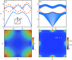
Figure 1: (color online). (a) Excitation spectra $E\left(k\right)$ (blue solid lines) and energy spectra of $h_{a}\left(k\right)$ (red dashed lines). (b) Excitation spectra $E\left(k_{2}\right)$ for the lattice model of $H_{\mathrm{BdG}}\left(k\right)$ in open-boundary condition. (c) Spin texture $\boldsymbol{l}\left(k\right)/\left|\boldsymbol{l}\left(k\right)\right|$ with the arrow representing $\left(l_{1},l_{2}\right)/\left|\boldsymbol{l}\right|$ and the color representing $l_{3}/\left|\boldsymbol{l}\right|$. (d) Berry curvature. Parameters: $\mu=-5$, $m=1$ and $\xi=2$.

We further numerically solve the effective single-particle via Eqs. (29–30). Assuming

$$h_{0}\left(k\right)=\lambda\mathbb{I}+\boldsymbol{l}\cdot\boldsymbol{\sigma},$$ (47)

where $\lambda\left(k\right)>0$ and $\boldsymbol{l}\left(k\right)\in\mathbb{R}^{3}\backslash 0$, we obtain values of $\lambda$ and $\boldsymbol{l}$ numerically. The spin texture $\boldsymbol{l}/\left|\boldsymbol{l}\right|$ and excitation spectra $E\left(k\right)=\lambda\pm\left|\boldsymbol{l}\right|$ for parameters $\mu=-5$, $\xi=2$ and $m=1$ are presented in Fig. 1 (a) and (c), respectively. We infer that $E\left(k\right)$ in Fig. 1 (a) opens a gap in the presence of the two-boson interactions. And the skyrmion in Fig. 1 (c) reflects the non-triviality of the interaction-driven phase. We also present the Berry curvature in Fig. 1 (d) and integrate it to gain the Chern number. The numerical result $\mathrm{CN}=1$ coincides with the analytical result of Eq. (46). Finally, we consider the lattice model of $H_{\mathrm{BdG}}\left(k\right)$ and adopt open and periodic boundary conditions along two othorgonal directions, respectively. Two edge modes inside the excitation gap are observed in the excitation spectra as shown in Fig. 1 (b). The presence of edge modes is closely related to the Chern number of the bulk Hamiltonian $H\left(k\right)$ Peano and Schulz-Baldes (2018), which is similar to the fermionic case.

IV.2 $\mathbb{Z}_{2}$-type model

We also propose a $\mathbb{Z}_{2}$-type topological phase in 2D and 3D based on the similar construction. We choose the BdG Hamiltonian with block matrices

$$h_{a}\left(k\right)=\sum_{j=1}^{d}\gamma^{j}\sin k_{j}-\mu\mathbb{I},\leavevmode\nobreak\ (\mu<0),$$ (48)

$$h_{x}\left(k\right)=\gamma^{0}\left(m+\sum_{j=1}^{d}\cos k_{j}\right)+\xi\mathbb{I},\leavevmode\nobreak\ (m,\xi\in\mathbb{R}).$$ (49)

Here $\gamma^{0},\gamma^{j}$ are the Clifford generators and $k_{j}\in\left[0,2\pi\right]$ form a $d$-dimensional torus ($d=2,3$). This model possesses all the $T,C,P$ symmetries and belongs to class HI. Its topological phases are classified by $\mathbb{Z}_{2}$ for both 2D and 3D. Similar to the above analysis, the $C$ symmetry and Kramer degeneracy from $T^{2}=-\mathbb{I}$ symmetry causes spectral degeneracy, so that the spectra consist of two separate bands. Then the gap-closing condition is also given by $H_{0}\left(k;\Omega\right)=\lambda\mathbb{I}$ which is equivalent to $\left(\tau H\right)^{2}=\lambda^{2}\mathbb{I}$. We can also prove that $H_{\mathrm{BdG}}\left(k\right)+\Omega\mathbb{I}\approx H_{\mathrm{BdG}}\left(k\right)$ and obtain a perturbative result

$$h_{0}\left(k\right)\approx h_{a}\left(k\right)-\frac{1}{2\Omega}h_{x}h_{x}^{\dagger}\left(k\right)+\Omega\mathbb{I}$$ (50)

in the limit of $\Omega\rightarrow\infty$. This single-particle Hamiltonian serves as a $T$-invariant topological insulator Bernevig (2013). When $\xi\neq 0$, topological non-trivial phases appear if $d-2<\left|m\right|<d$ and trivial phases emerge if $\left|m\right|>d$ or $\left|m\right|<d-2$.

V Conclusions

We have accomplished the symmetry and topological classification of the QBS with an excitation band gap. Three basic symmetries in QBS are introduced and the ten-fold symmetry classification is realized. A specific decomposition of the elementary-excitation Hamiltonian is applied to reveal its algebraic and topological structures. Then the classification table of excitations in QBS is derived based on that of AZ classes. Unique topological phases of bosons are discussed and concrete bosonic models without fermionic counterpart are constructed. Our work provides a framework to explore richer topological physics of bosons.

The possible studies in future include the implementation of the predicted topological phases in realistic systems, the extension of the classification table by considering lattice symmetries, and a systematical investigation on the bulk-edge correspondence in the bosonic case.

Appendix A Classification principle

We briefly introduce the classification principle of AZ classes for free-fermion systems and extend it to our quadratic bosonic systems. For the fermionic AZ classes, usually one first introduces the trivial Hamiltonian

$$\sigma=\left(\begin{array}[]{cc}\mathbb{I}_{r}\\ &-\mathbb{I}_{r}\end{array}\right),$$ (51)

which corresponds to a flat-band system with equal conduction and valence bands. Next, we apply K-theory to define the stable equivalence of single-particle Hamiltonians $h\left(k\right)$ and $h^{\prime}\left(k\right)$ as follows,

$$h\left(k\right)\oplus\sigma\approx h^{\prime}\left(k\right)\oplus\sigma^{\prime},$$ (52)

where $\sigma$ and $\sigma^{\prime}$ are independent trivial Hamiltonians with unlimited matrix sizes. The stable equivalence studies the homotopy of Hamiltonians whose intrinsic space is enlarged to $\infty$-dimension by attaching flat bands. It is a looser condition than the original homotopy such that the classification becomes much easier.

People usually regard the stably equivalent class $\left[h\left(k\right)\right]$ as a topological phase and achieve the classification by counting out all the $\left[h\left(k\right)\right]$ for given symmetries and $k$-space dimension Chiu et al. (2016); Kitaev (2009). The classification table is derived from the Bott periodicity theorem Stone et al. (2011). The results of class A, AI, and AII are presented in Tab. 3, where the $k$-space is chosen as sphere $S^{d}$. If the $k$-space becomes the usual torus $T^{d}$ in band theory, the final result is the present answer plus some weak topological invariants Kitaev (2009).

Table 3: Topological classification of class A, AI, and AII. The $k$-space is chosen as sphere $S^{d}$. In the second column, symbol 0 refers to absence of symmetry and $\pm$ refers to the presence of symmetry with $T^{2}=\pm\mathbb{I}$.

AZ class	$T$	Classifying space	$d=$0	1	2	3	4	5	6	7
A	0	$\mathcal{C}_{0}=\mathbb{Z}\times BU$	$\mathbb{Z}$	$0$	$\mathbb{Z}$	$0$	$\mathbb{Z}$	$0$	$\mathbb{Z}$	$0$
AI	+	$\mathcal{R}_{0}=\mathbb{Z}\times BO$	$\mathbb{Z}$	$0$	$0$	$0$	$\mathbb{Z}$	$0$	$\mathbb{Z}_{2}$	$\mathbb{Z}_{2}$
AII	-	$\mathcal{R}_{4}=\mathbb{Z}\times BSp$	$\mathbb{Z}$	$0$	$\mathbb{Z}_{2}$	$\mathbb{Z}_{2}$	$\mathbb{Z}$	$0$	$0$	$0$

For the quadratic bosonic system, we naturally extend the trivial Hamiltonian $O$ as follows,

$$O=\left(\begin{array}[]{cc}o_{\tau=+1}\\ &o_{\tau=-1}\end{array}\right),\leavevmode\nobreak\ o=\left(\begin{array}[]{cc}E_{\mathrm{up}}\mathbb{I}_{r}\\ &E_{\mathrm{low}}\mathbb{I}_{r}\end{array}\right),$$ (53)

where the block matrix $o_{\tau=\pm 1}$ acting on the $\tau=\pm 1$ eigenspace corresponds to a flat-band subsystem with equal upper and lower excitation bands (the excitation bands above and below the gap). Hence, attaching it on $H\left(k\right)$ does not change the sign difference of $\tau$ nor the difference of upper/lower band numbers. We thus call $H\left(k\right)$ is stably equivalent to $H^{\prime}\left(k\right)$ if

$$H\left(k\right)\oplus O\approx H^{\prime}\left(k\right)\oplus O^{\prime},$$ (54)

denoted as $H\left(k\right)\sim H^{\prime}\left(k\right)$. We regard the stable equivalent class $\left[H\left(k\right)\right]$ as a topological phase and achieve the classification by counting out all the $\left[H\left(k\right)\right]$. Since the homotopic property of $H\left(k\right)$ is determined by $h_{0}\left(k\right)$ or $h_{0}\left(k\right)\oplus h_{0}^{\prime}\left(k\right)$, the classification of $\left[H\left(k\right)\right]$ reduces to the classification of $\left[h_{0}\left(k\right)\right]$ or $\left[h_{0}\left(k\right)\oplus h_{0}^{\prime}\left(k\right)\right]$. The stable equivalence for subsystems $h_{0}\left(k\right)$ and $h_{0}^{\prime\prime}\left(k\right)$ is reduced from Eq. (54), given by

$$h_{0}\left(k\right)\oplus o\approx h_{0}^{\prime\prime}\left(k\right)\oplus o^{\prime\prime}.$$ (55)

We know that $h_{0}\left(k\right)$ is attributed to class A, AI, or AII, and $o$ is homotopic to the fermionic trivial Hamiltonian $\sigma$. Therefore, the classification of $\left[h_{0}\left(k\right)\right]$ is directly given by the periodic table of AZ classes Tab. 3. For independent $h_{0}\left(k\right)$ and $h_{0}^{\prime}\left(k\right)$, the classification of $\left[h_{0}\left(k\right)\oplus h_{0}^{\prime}\left(k\right)\right]=\left[h_{0}\left(k\right)\right]\oplus\left[h_{0}^{\prime}\left(k\right)\right]$ simply gets doubled.

Appendix B Characteristic numbers

We provide the computation formulas of the Chern number, Chern-Simons invariant, and Fu-Kane invariant for the single-particle Hamiltonians $h_{0}\left(k\right)$ and $h_{0}^{\prime}\left(k\right)$Chiu et al. (2016). Firstly, the Chern number is defined by

$$\mathrm{CN}=\int_{\mathrm{BZ}}\det\left(\mathbb{I}+\frac{i}{2\pi}\mathcal{F}\right),$$ (56)

where $\mathcal{F}=\mathrm{d}\mathcal{A}+\mathcal{A}\land\mathcal{A}$ is the Berry curvature 2-form. Here $\mathcal{A}$ denotes the Berry connection form of the bands below the gap, and BZ refers to the Brillouin zone, namely, the $k$-space. It is a topological invariant that measures the twisting of the energy bands (vector bundle). Secondly, the Chern-Simons invariant for $d=2m-1$ is a geometrical invariant defined by

$$\mathrm{CS}=\exp\left(2\pi i\int_{\mathrm{BZ}}\mathrm{cs}_{m}\right).$$ (57)

The Chern-Simons form reads

$$\mathrm{cs}_{m}=\frac{1}{\left(m-1\right)!}\left(\frac{i}{2\pi}\right)^{m}\int_{0}^{1}\mathrm{d}t\mathrm{Tr}\left(\mathcal{A}\land\mathcal{F}_{t}^{m-1}\right),$$ (58)

where $\mathcal{F}_{t}=t\mathrm{d}\mathcal{A}+t^{2}\mathcal{A}^{2}$. With the existence of time-reversal symmetry, $\mathrm{CS}$ takes discrete values $\pm 1$ for $d=3,7$ and then keeps invariant under the continuous deformation of $\mathcal{A}\left(k\right)$, which becomes a topological invariant. Thirdly, the Fu-Kane invariant for $d=2m$ is defined by

$$\mathrm{FK}=\int_{\mathrm{BZ}/2}\frac{1}{m!}\mathrm{Tr}\left(\frac{i}{2\pi}\mathcal{F}\right)^{m}-\int_{\partial\mathrm{BZ}/2}\mathrm{cs}_{m},$$ (59)

in which $\mathrm{BZ}/2$ refers to a half of Brillouin zone. It also takes discrete values $\pm 1$ for $d=2,6$ with the existence of the $T$ symmetry and thus becomes a topological invariant.

Finally, we provide the expressions of the Berry connection. Without loosing generality, we suppose the first $n$ elements of $E=u_{a}^{\dagger}h_{0}u_{a}$ lower than the energy gap. Then the Berry connection form of $h_{0}\left(k\right)$ is given by

$$\mathcal{A}=\Gamma^{\dagger}u_{a}^{\dagger}\mathrm{d}u_{a}\Gamma,\leavevmode\nobreak\ \Gamma^{\dagger}=\left(\begin{array}[]{cc}\mathbb{I}_{n}&0\end{array}\right).$$ (60)

Similarly, we suppose that the first $n^{\prime}$ elements of $e^{\prime}=u_{b}^{\dagger}h_{0}^{\prime}u_{b}$ are lower than the energy gap. Then the Berry connection of $h_{0}^{\prime}\left(k\right)$ is given by

$$\mathcal{A}^{\prime}=\Gamma^{\prime\dagger}u_{b}^{\dagger}\mathrm{d}u_{b}\Gamma^{\prime},\leavevmode\nobreak\ \Gamma^{\prime\dagger}=\left(\begin{array}[]{cc}\mathbb{I}_{n^{\prime}}&0\end{array}\right).$$ (61)

It is worthy to mention that in previous literature, a bosonic-version Berry connection is defined via the pseudo-unitary diagonalization Shindou et al. (2013), i.e.,

$$\mathcal{A}_{\mathrm{Bose}}=\left(\Gamma^{\dagger},0\right)V^{\dagger}\tau\mathrm{d}V\left(\begin{array}[]{c}\Gamma\\ 0\end{array}\right).$$ (62)

In fact, $\mathcal{A}_{\mathrm{Bose}}$ can be continuously mapped to $\mathcal{A}$ when $W\left(k\right)$ gradually decreases to zero. Since continuous mapping does not change the topology, these two Berry connections lead to the identical topological invariant.

References

- Haldane (1988) F. D. M. Haldane, Phys. Rev. Lett. 61, 2015 (1988).
- Kane and Mele (2005a) C. L. Kane and E. J. Mele, Phys. Rev. Lett. 95, 146802 (2005a).
- Kane and Mele (2005b) C. L. Kane and E. J. Mele, Phys. Rev. Lett. 95, 226801 (2005b).
- Bernevig et al. (2006) B. A. Bernevig, T. L. Hughes, and S.-C. Zhang, Science 314, 1757 (2006).
- Fu and Kane (2007) L. Fu and C. L. Kane, Phys. Rev. B 76, 045302 (2007).
- Read and Green (2000) N. Read and D. Green, Phys. Rev. B 61, 10267 (2000).
- Kitaev (2001) A. Y. Kitaev, Phys.-Usp. 44, 131 (2001).
- Mourik et al. (2012) V. Mourik, K. Zuo, S. M. Frolov, S. R. Plissard, E. P. A. M. Bakkers, and L. P. Kouwenhoven, Science 336, 1003 (2012).
- Sato and Ando (2017) M. Sato and Y. Ando, Rep. Prog. Phys. 80, 076501 (2017).
- Altland and Zirnbauer (1997) A. Altland and M. R. Zirnbauer, Phys. Rev. B 55, 1142 (1997).
- Zirnbauer (2010) M. R. Zirnbauer, ArXiv e-prints (2010), arXiv:1001.0722 [math-ph] .
- Stone et al. (2011) M. Stone, C.-K. Chiu, and A. Roy, J. Phys. A: Math. Theor. 44, 045001 (2011).
- Kitaev (2009) A. Kitaev, AIP Conf. Proc. 1134, 22 (2009).
- Zhao and Wang (2013) Y. X. Zhao and Z. D. Wang, Phys. Rev. Lett. 110, 240404 (2013).
- Chiu et al. (2016) C.-K. Chiu, J. C. Y. Teo, A. P. Schnyder, and S. Ryu, Rev. Mod. Phys. 88, 035005 (2016).
- Chang (2018) P.-Y. Chang, Phys. Rev. B 97, 224304 (2018).
- Yang et al. (2018) C. Yang, L. Li, and S. Chen, Phys. Rev. B 97, 060304 (2018).
- Gong and Ueda (2018) Z. Gong and M. Ueda, Phys. Rev. Lett. 121, 250601 (2018).
- Qiu et al. (2018) X. Qiu, T.-S. Deng, G.-C. Guo, and W. Yi, Phys. Rev. A 98, 021601 (2018).
- Shen et al. (2018) H. Shen, B. Zhen, and L. Fu, Phys. Rev. Lett. 120, 146402 (2018).
- Kawabata et al. (2018) K. Kawabata, K. Shiozaki, and M. Ueda, Phys. Rev. B 98, 165148 (2018).
- Yao and Wang (2018) S. Yao and Z. Wang, Phys. Rev. Lett. 121, 086803 (2018).
- Yao et al. (2018) S. Yao, F. Song, and Z. Wang, Phys. Rev. Lett. 121, 136802 (2018).
- Kawabata et al. (2019a) K. Kawabata, S. Higashikawa, Z. Gong, Y. Ashida, and M. Ueda, Nat. Commun. 10, 297 (2019a).
- Roy and Harper (2017) R. Roy and F. Harper, Phys. Rev. B 96, 155118 (2017).
- Gong et al. (2018) Z. Gong, Y. Ashida, K. Kawabata, K. Takasan, S. Higashikawa, and M. Ueda, Phys. Rev. X 8, 031079 (2018).
- Kawabata et al. (2019b) K. Kawabata, K. Shiozaki, M. Ueda, and M. Sato, Phys. Rev. X 9, 041015 (2019b).
- Haldane and Raghu (2008) F. D. M. Haldane and S. Raghu, Phys. Rev. Lett. 100, 013904 (2008).
- Wang et al. (2008) Z. Wang, Y. D. Chong, J. D. Joannopoulos, and M. Soljačić, Phys. Rev. Lett. 100, 013905 (2008).
- Chong et al. (2008) Y. D. Chong, X.-G. Wen, and M. Soljačić, Phys. Rev. B 77, 235125 (2008).
- Hafezi et al. (2011) M. Hafezi, E. A. Demler, M. D. Lukin, and J. M. Taylor, Nat. Phys. 7, 907 (2011).
- Hafezi et al. (2013) M. Hafezi, S. Mittal, J. Fan, A. Migdall, and J. M. Taylor, Nat. Photonics 7, 1001 (2013).
- Poo et al. (2011) Y. Poo, R.-x. Wu, Z. Lin, Y. Yang, and C. T. Chan, Phys. Rev. Lett. 106, 093903 (2011).
- Poo et al. (2016) Y. Poo, C. He, C. Xiao, M.-H. Lu, R.-X. Wu, and Y.-F. Chen, Sci. Rep. 6, 29380 (2016).
- Skirlo et al. (2014) S. A. Skirlo, L. Lu, and M. Soljačić, Phys. Rev. Lett. 113, 113904 (2014).
- Skirlo et al. (2015) S. A. Skirlo, L. Lu, Y. Igarashi, Q. Yan, J. Joannopoulos, and M. Soljačić, Phys. Rev. Lett. 115, 253901 (2015).
- Wang et al. (2009) Z. Wang, Y. Chong, J. D. Joannopoulos, and M. Soljačić, Nature 461, 772 (2009).
- Aidelsburger et al. (2013) M. Aidelsburger, M. Atala, M. Lohse, J. T. Barreiro, B. Paredes, and I. Bloch, Phys. Rev. Lett. 111, 185301 (2013).
- Aidelsburger et al. (2014) M. Aidelsburger, M. Lohse, C. Schweizer, M. Atala, J. Barreiro, S. Nascimbène, N. Cooper, I. Bloch, and N. Goldman, Nat. Phys. 11, 162 (2014).
- Ring and Schuck (1980) P. Ring and P. Schuck, The Nuclear Many-Body Problem (Springer, New York, 1980).
- Rossignoli and Kowalski (2005) R. Rossignoli and A. M. Kowalski, Phys. Rev. A 72, 032101 (2005).
- Blaizot and Ripka (1986) J. P. Blaizot and G. Ripka, Quantum Theory of Finite Systems (MIT Press, Cambridge, MA, 1986).
- Shindou et al. (2013) R. Shindou, R. Matsumoto, S. Murakami, and J.-i. Ohe, Phys. Rev. B 87, 174427 (2013).
- Chisnell et al. (2015) R. Chisnell, J. S. Helton, D. E. Freedman, D. K. Singh, R. I. Bewley, D. G. Nocera, and Y. S. Lee, Phys. Rev. Lett. 115, 147201 (2015).
- Roldán-Molina et al. (2016) A. Roldán-Molina, A. S. Nunez, and J. Fernández-Rossier, New J. Phys. 18, 045015 (2016).
- Díaz et al. (2019) S. A. Díaz, J. Klinovaja, and D. Loss, Phys. Rev. Lett. 122, 187203 (2019).
- Kondo et al. (2019) H. Kondo, Y. Akagi, and H. Katsura, Phys. Rev. B 99, 041110 (2019).
- Kondo et al. (2019) H. Kondo, Y. Akagi, and H. Katsura, arXiv e-prints , arXiv:1905.06748 (2019), arXiv:1905.06748 [cond-mat.mes-hall] .
- Bardyn et al. (2016) C.-E. Bardyn, T. Karzig, G. Refael, and T. C. H. Liew, Phys. Rev. B 93, 020502 (2016).
- Peano et al. (2016) V. Peano, M. Houde, C. Brendel, F. Marquardt, and A. A. Clerk, Nat. Commun. 7, 10779 (2016).
- Engelhardt and Brandes (2015) G. Engelhardt and T. Brandes, Phys. Rev. A 91, 053621 (2015).
- Xu et al. (2016) Z.-F. Xu, L. You, A. Hemmerich, and W. V. Liu, Phys. Rev. Lett. 117, 085301 (2016).
- Di Liberto et al. (2016) M. Di Liberto, A. Hemmerich, and C. Morais Smith, Phys. Rev. Lett. 117, 163001 (2016).
- Luo et al. (2018) G.-Q. Luo, A. Hemmerich, and Z.-F. Xu, Phys. Rev. A 98, 053617 (2018).
- Colpa (1986) J. H. P. Colpa, Physica A: Statistical Mechanics and its Applications 134, 417 (1986).
- Simon et al. (1999) R. Simon, S. Chaturvedi, and V. Srinivasan, J. Math. Phys. 40, 3632 (1999).
- Yan and Zhou (2018) Y. Yan and Q. Zhou, Phys. Rev. Lett. 120, 235302 (2018).
- Lan et al. (2018) T. Lan, L. Kong, and X.-G. Wen, Phys. Rev. X 8, 021074 (2018).
- Lan and Wen (2019) T. Lan and X.-G. Wen, Phys. Rev. X 9, 021005 (2019).
- (60) A deformation retraction satisfies that (1) is an identity mapping; (2) is a retraction mapping; (3) is identity mapping for each .
- Peano and Schulz-Baldes (2018) V. Peano and H. Schulz-Baldes, J. Math. Phys. 59, 031901 (2018).
- Lein and Sato (2019) M. Lein and K. Sato, Phys. Rev. B 100, 075414 (2019).
- Scully and Zubairy (1997) M. O. Scully and M. S. Zubairy, Quantum Optics (Cambridge University Press, 1997).
- Qi et al. (2006) X.-L. Qi, Y.-S. Wu, and S.-C. Zhang, Phys. Rev. B 74, 045125 (2006).
- Bernevig (2013) B. A. Bernevig, Topological Insulators and Topolocial Superconductors (Princeton University Press, 2013).