Gradient tree boosting with random output projections for multi-label classification and multi-output regression

Abstract

In many applications of supervised learning, multiple classification or regression outputs have to be predicted jointly. We consider several extensions of gradient boosting to address such problems. We first propose a straightforward adaptation of gradient boosting exploiting multiple output regression trees as base learners. We then argue that this method is only expected to be optimal when the outputs are fully correlated, as it forces the partitioning induced by the tree base learners to be shared by all outputs. We then propose a novel extension of gradient tree boosting to specifically address this issue. At each iteration of this new method, a regression tree structure is grown to fit a single random projection of the current residuals and the predictions of this tree are fitted linearly to the current residuals of all the outputs, independently. Because of this linear fit, the method can adapt automatically to any output correlation structure. Extensive experiments are conducted with this method, as well as other algorithmic variants, on several artificial and real problems. Randomly projecting the output space is shown to provide a better adaptation to different output correlation patterns and is therefore competitive with the best of the other methods in most settings. Thanks to model sharing, the convergence speed is also improved, reducing the computing times (or the complexity of the model) to reach a specific accuracy.

1 Introduction

Multi-output supervised learning aims to model input-output relationships from observations of input-output pairs whenever the output space is a vector of random variables. Multi-output classification and regression tasks have numerous applications in domains ranging from biology to multimedia, and recent applications in this area correspond to very high dimensional output spaces Agrawal et al (2013); Dekel and Shamir (2010).

Classification and regression trees Breiman et al (1984) are popular supervised learning methods that provide state-of-the-art performance when exploited in the context of ensemble methods, namely Random forests Breiman (2001); Geurts et al (2006) and Boosting Freund and Schapire (1997); Friedman (2001). Classification and regression trees can obviously be exploited to handle multi-output problems. The most straightforward way to address multi-output tasks is to apply standard single output methods separately and independently on each output. Although simple, this method, called binary relevance Tsoumakas et al (2009) in multi-label classification or single target Spyromitros-Xioufis et al (2012) in multi-output regression is often suboptimal as it does not exploit potential correlations that might exist between the outputs. Tree ensemble methods have however been explicitely extended by several authors to the joint prediction of multiple outputs (e.g., Segal, 1992; Blockeel et al, 2000). These extensions build a single tree to predict all outputs at once. They adapt the score measure used to assess splits during the tree growth to take into account all outputs and label each tree leaf with a vector of values, one for each output. Like standard classification or regression trees, multiple output trees can be exploited in the context of random forests Barutcuoglu et al (2006); Joly et al (2014); Kocev et al (2007, 2013); Segal and Xiao (2011); Haider et al (2015) or boosting Geurts et al (2007) ensembles, which often offer very significant accuracy improvements with respect to single trees. Multiple output trees have been shown to be competitive with other multiple output methods Madjarov et al (2012), but, to the best of our knowledge, it has not been studied as extensively in the context of gradient tree boosting.

Binary relevance / single target of single output tree models and multiple output tree models represent two extremes in terms of tree structure learning: the former builds a separate tree ensemble structure for each output, while the latter builds a single tree ensemble structure for all outputs. Building separate ensembles for each output may be rather inefficient when the outputs are strongly correlated. Correlations between the outputs could indeed be exploited either to reduce model complexity (by sharing the tree structures between several outputs) or to improve accuracy by regularization. Trying to fit a single tree structure for all outputs seems however counterproductive when the outputs are independent. Indeed, in the case of independent outputs, simultaneously fitting all outputs with a single tree structure may require a much more complex tree structure than the sum of the individual tree complexities required to fit the individual outputs. Since training a more complex tree requires a larger learning sample, multiple output trees are expected to be outperformed by binary relevance / single target in this situation.

In this paper, we first formally adapt gradient boosting to multiple output tasks. We then propose a new method that aims at circumventing the limitations of both binary relevance / single target and multiple output methods, in the specific context of tree-based base-learners. Our method is an extension of gradient tree boosting that can adapt itself to the presence or absence of correlations between the outputs. At each boosting iteration, a single regression tree structure is grown to fit a single random projection of the outputs, or more precisely, of their residuals with respect to the previously built models. Then, the predictions of this tree are fitted linearly to the current residuals of all the outputs (independently). New residuals are then computed taking into account the resulting predictions and the process repeats itself to fit these new residuals. Because of the linear fit, only the outputs that are correlated with the random projection at each iteration will benefit from a reduction of their residuals, while outputs that are independent of the random projection will remain mostly unaffected. As a consequence, tree structures will only be shared between correlated outputs as one would expect. Another variant that we explore consists in replacing the linear global fit by a relabelling of all tree leaves for each output in turn.

The paper is structured as follows. We show how to extend the gradient boosting algorithms to multi-output tasks in Section 3. We provide for these algorithms a convergence proof on the training data and discuss the effect of the random projection of the output space. We study empirically the proposed approach in Section 4. Our first experiments compare the proposed approaches to binary relevance / single target on artificial datasets where the output correlation is known. We also highlight the effect of the choice and size of the random projection space. We finally carry out an empirical evaluation of these methods on 21 real-world multi-label and 8 multi-output regression tasks. Section 5 discusses related works and Section 6 presents our conclusions.

2 Background

We denote by $\cal{X}$ an input space, and by $\mathcal{Y}$ an output space; we suppose that $\mathcal{X}=\mathbb{R}^{p}$ (where $p$ denotes the number of input features), and that $\mathcal{Y}=\mathbb{R}^{d}$ (where $d$ is the dimension of the output space). We denote by $P_{{\cal X},{\cal Y}}$ the joint (unknown) sampling density over $\mathcal{X}\times\mathcal{Y}$. Given a learning sample $\left((x^{i},y^{i})\in\left(\mathcal{X}\times\mathcal{Y}\right)\right)_{i=1}^{n}$ of $n$ observations in the form of input-output pairs, a supervised learning task is defined as searching for a function $f^{*}:\mathcal{X}\rightarrow\mathcal{Y}$ in a hypothesis space $\mathcal{H}\subset\mathcal{Y}^{\mathcal{X}}$ that minimizes the expectation of some loss function $\ell:\mathcal{Y}\times\mathcal{Y}\rightarrow\mathbb{R}$ over the joint distribution of input / output pairs: $f^{*}\in\arg\min_{f\in\mathcal{H}}E_{P_{{\cal X},{\cal Y}}}\{\ell(f(x),y)\}$.

NOTATIONS: Superscript indices ($x^{i},y^{i}$) denote (input, output) vectors of an observation $i\in\{1,\ldots,n\}$. Subscript indices (e.g. $x_{j},y_{k}$) denote components of vectors.

We present single and multiple output decision trees in Section 2.1, gradient boosting in Section 2.2 and random projections in Section 2.3.

2.1 Single and multiple output decision trees and forests

A decision tree model Breiman et al (1984) is a hierarchical set of questions leading to a prediction. The internal nodes, also called test nodes, test the value of a feature. A test node $N_{t}$ has two children called the left child and the right child; it furthermore has a splitting rule $s_{t}$ testing whether or not a sample belongs to its left or right child. For a continuous or categorical ordered input, the splitting rules are typically of the form $s_{t}(x)=x_{F_{t}}\leq\tau_{t}$ testing whether or not the input value $x_{F_{t}}$ is smaller or equal to a constant $\tau_{t}$. For a binary or categorical input, the splitting rule is of the form $s_{t}(x)=x_{F_{t}}\in B_{t}$ testing whether or not the input value $x_{F_{t}}$ belongs to the subset of values $B_{t}$. To predict an unseen sample, one starts at the root node and follows the tree structure until reaching a leaf labelled with a prediction $\beta_{t}\in\mathcal{Y}$.

Random forests.

Single decision trees are often not very accurate because of a very high variance. One way to reduce this variance is to grow instead an ensemble of several randomized trees and then to average their predictions. For example, Breiman (2001)’s random forests method builds an ensemble of trees where each tree is trained on a bootstrap copy of the training set and the best split selection is randomized by searching this split among $k$ features randomly selected at each node among the $p$ original features ($k\leq p$). This randomization can be applied in both single and multi-output settings Kocev et al (2007); Segal and Xiao (2011); Joly et al (2014). In what follows, we will compare our gradient boosting approaches with both binary relevance / single target of single output random forests and with multi-output random forests.

2.2 Gradient boosting

Boosting methods fit additive models of the following form:

$$f(x)=\sum_{m=1}^{M}\alpha_{m}f_{m}(x),$$ (1)

where $\{f_{m}\}_{m=1}^{M}$ are $M$ weak models, so as to minimize some loss function $\ell:\mathcal{Y}\times\mathcal{Y}\rightarrow\mathbb{R}^{+}$ over the learning sample. This additive model is fit sequentially using a forward stagewise strategy, adding at each step a new model $f_{m}(x)$, together with its weight $\alpha_{m}$, to the previous $m-1$ models so as to minimize the loss over the learning sample:

$$\min_{\alpha_{m},f_{m}\in\mathbb{R}\times\mathcal{H}}\sum_{(x,y)\in\mathcal{L}}\ell\left(y,\sum_{l=1}^{m-1}\alpha_{l}f_{l}(x)+\alpha_{m}f_{m}(x)\right),$$ (2)

where $\cal H$ is the hypothesis space of all candidate base functions, e.g., the set of all regression trees of some maximum depth. Solving (2) is however difficult for general loss function. Inspired by gradient descent, gradient boosting Friedman (2001) replaces the direct resolution of (2) by a single gradient descent step in the functional space and therefore can be applied for any differentiable loss function. The whole procedure is detailed in Algorithm 1. Starting from an initial constant estimate $\rho_{0}\in\mathbb{R}$ (line 2), gradient boosting iteratively follows the negative gradient of the loss $\ell$ (computed in line 4) as estimated by a regression model $g_{m}$ fitted over the training samples using least-square (line 5) and using an optimal step length $\rho_{m}$ minimizing the loss $\ell$ (computed in line 6). Independently of the loss, the base model is fitted using least-square and the algorithm can thus exploit any supervised learning algorithm that accept square loss to obtain the individual models, e.g., standard regression trees.

Algorithm 1 Gradient boosting algorithm

1:function GradientBoosting($\mathcal{L}=\{(x^{i},y^{i})\in\mathcal{X}\times\mathcal{Y}\}_{i=1}^{n};\ell;\mathcal{H};M$)

2:     $f_{0}(x)=\rho_{0}=\arg\min_{\rho\in\mathbb{R}}\sum_{i=1}^{n}\ell(y^{i},\rho)$.

3:     for $m$ = 1 to $M$ do

4:         Compute the loss gradient for the training set points

$$\quad g_{m}^{i}=\left[\frac{\partial}{\partial y^{\prime}}\ell(y^{i},y^{\prime})\right]_{y^{\prime}=f_{m-1}(x)}\forall i\in\left\{1,\ldots,n\right\}.$$

5:         Find a correlated direction to the loss gradient

$$\quad g_{m}=\arg\min_{g\in\mathcal{H}}\sum_{i=1}^{n}(-g_{m}^{i}-g(x^{i}))^{2}.$$

6:         Find an optimal step length in the direction $g_{m}$

$$\quad\rho_{m}=\arg\min_{\rho\in\mathbb{R}}\sum_{i=1}^{n}\ell\left(y^{i},f_{m-1}(x^{i})+\rho g_{m}(x^{i})\right).$$

7:         $f_{m}(x)=f_{m-1}(x)+\mu\rho_{m}g_{m}(x)$.

8:     end for

9:     return $f_{M}(x)$

10:end function

The algorithm is completely defined once we have (i) the constant minimizing the chosen loss (line 4) and (ii) the gradient of the loss (line 2). Table 1 shows these two elements for the square loss in regression and the exponential loss in classification, as these two losses will be exploited later in our experiments. With square loss, step 4 actually simply fits the actual residuals of the problem and the algorithm is called least-squares regression boosting Hastie et al (2005). With exponential loss, the algorithm reduces to the exponential classification boosting algorithm of Zhu et al (2009). Friedman (2001) gives the details how to handle loss functions such as the absolute loss or the logistic loss.

The optimal step length (line 6 of Algorithm 1) can be computed either analytically as for the square loss (see Section 3.3.1) or numerically using, e.g., Brent (2013)’s method, a robust root-finding method allowing to minimize single unconstrained optimization problem, as for the exponential loss. Friedman (2001) advises to use one step of the Newton-Raphson method. However, the Newton-Raphson algorithm might not converge if the first and second derivatives of the loss are small. These conditions occur frequently in highly imbalanced supervised learning tasks.

A learning rate $\mu\in(0,1]$ is often added (line 7) to shrink the size of the gradient step $\rho_{m}$ in the residual space in order to avoid overfitting the learning sample. Another possible modification is to introduce randomization, e.g. by subsampling without replacement the samples available (from all learning samples) at each iteration Friedman (2002). In our experiment with trees, we will introduce randomization by growing the individual trees with the feature randomization of random forests (parameterized by the number of features $k$ randomly selected at each node).

Table 1: Constant minimizers and gradient of square loss in regression ($\mathcal{Y}=\mathbb{R}$) and exponential loss in binary classification ($\mathcal{Y}=\{-1,1\}$).

Loss	$\ell(y,y^{\prime})$	$f_{0}(x)$	$-\partial{}\ell(y,y^{\prime})/\partial{}y^{\prime}$
Square	$\frac{1}{2}(y-y^{\prime})^{2}$	$\frac{1}{n}\sum_{i=1}^{n}y^{i}$	$y-y^{\prime}$
Logistic	$\log(1+\exp(-2yy^{\prime}))$	$\log\left(\frac{\sum_{i=1}^{n}1(y^{i}=1)}{\sum_{i=1}^{n}1(y^{i}=-1)}\right)$	$\frac{2y}{1+\exp(2yy^{\prime})}$

2.3 Random projections

Random projection is a very simple and efficient way to reduce the dimensionality of a high-dimensional space. The general idea of this technique is to map each data vector $y$ initially of size $d$ into a new vector $\Phi y$ of size $q$ by multiplying this vector by a matrix $\Phi$ of size $q\times d$ drawn randomly from some distribution. Since the projection matrix is random, it can be generated very efficiently. The relevance of the technique in high-dimensional spaces originates from the Johnson-Lindenstrauss lemma, which is stated as follows:

Lemma 1

Johnson and Lindenstrauss (1984) Given $\epsilon>0$ and an integer $n$, let $q$ be a positive integer such that $q>8\epsilon^{-2}\ln{n}$. For any sample $(y^{i})_{i=1}^{n}$ of $n$ points in $\mathbb{R}^{d}$ there exists a matrix $\Phi\in\mathbb{R}^{q\times d}$ such that for all $i,j\in\{1,\ldots,n\}$

$$(1-\epsilon)||y^{i}-y^{j}||^{2}\leq||\Phi y^{i}-\Phi y^{j}||^{2}\leq(1+\epsilon)||y^{i}-y^{j}||^{2}.$$ (3)

This lemma shows that when the dimension of the data is high, it is always possible to map linearly the data into a low-dimensional space where the original distances are preserved. When $d$ is sufficiently large, it has been shown that matrices that satisfy Equation 3 with high probability can be generated randomly in several ways. For example, this is the case of the following two families of random matrices Achlioptas (2003):

• Gaussian matrices whose elements are drawn i.i.d. in $\mathcal{N}(0,1/q)$;

• (sparse) Rademacher matrices whose elements are drawn in the finite set $\left\{-\sqrt{\frac{s}{q}},0,\sqrt{\frac{s}{q}}\right\}$ with probability $\left\{\frac{1}{2s},1-\frac{1}{s},\frac{1}{2s}\right\}$, where $1/s\in(0,1]$ controls the sparsity of $\Phi$.

When $s=3$, Rademacher projections will be called Achlioptas random projections Achlioptas (2003). When the size of the original space is $p$ and $s=\sqrt{p}$, then we will call the resulting projections sparse random projections as in Li et al (2006). Formal proofs that these random matrices all satisfy Equation 3 with high probability can be found in the corresponding papers. In all cases, the probability of satisfying Equation 3 increases with the number of random projections $q$. The choice of $q$ is thus a trade-off between the quality of the approximation and the size of the resulting embedding.

Note that selecting randomly $q$ dimensions among the original ones is also a random projection scheme. The corresponding projection matrix $\Phi$ is obtained by sub-sampling (with or without replacement) q rows from the $d\times d$ identity matrix Candes and Plan (2011). Later in the paper, we will call this random projection random output sub-sampling.

3 Gradient boosting with multiple outputs

Starting from a multi-output loss, we first show in Section 3.1 how to extend the standard gradient boosting algorithm to solve multi-output tasks, such as multi-output regression and multi-label classification, by exploiting existing weak model learners suited for multi-output prediction. In Section 3.2, we then propose to combine single random projections of the output space with gradient boosting to automatically adapt to the output correlation structure on these tasks. This constitutes the main methodological contribution of the paper. We discuss and compare the effect of the random projection of the output space in Section 3.3. Note that we give a convergence proof on the training data for the proposed algorithms in Appendix A.

3.1 Standard extension of gradient boosting to multi-output tasks

A loss function $\ell(y,y^{\prime})\in\mathbb{R}^{+}$ computes the difference between a ground truth $y$ and a model prediction $y^{\prime}$. It compares scalars with single output tasks and vectors with multi-output tasks. The two most common regression losses are the square loss $\ell_{square}(y,y^{\prime})=\frac{1}{2}(y-y^{\prime})^{2}$ and the absolute loss $\ell_{absolute}(y,y)=|y-y^{\prime}|$. Their multi-output extensions are the $\ell_{2}$-norm and $\ell_{1}$-norm losses:

$$\ell_{2}(y,y^{\prime}) =\frac{1}{2}||y-y^{\prime}||_{\ell_{2}}^{2},$$ (4)

$$\ell_{1}(y,y^{\prime}) =||y-y^{\prime}||_{\ell_{1}}.$$ (5)

In classification, the most commonly used loss to compare a ground truth $y$ to the model prediction $f(x)$ is the $0-1$ loss $\ell_{0-1}(y,y^{\prime})=1(y\not=y^{\prime})$, where $1$ is the indicator function. It has two standard multiple output extensions (i) the Hamming loss $\ell_{Hamming}$ and (ii) the subset $0-1$ loss $\ell_{\text{subset }0-1}$:

$$\ell_{Hamming}(y,y^{\prime}) =\sum_{j=1}^{d}1(y_{j}\not=y^{\prime}_{j}),$$ (6)

$$\ell_{\text{subset }0-1}(y,y^{\prime}) =1(y\not=y^{\prime}).$$ (7)

Since these losses are discrete, they are non-differentiable and difficult to optimize. Instead, we propose to extend the logistic loss $\ell_{logistic}(y,y^{\prime})=\log(1+\exp(-2yy^{\prime}))$ used for binary classification tasks to the multi-label case, as follows:

$$\ell_{logistic}(y,y^{\prime})=\sum_{j=1}^{d}\log(1+\exp(-2y_{j}y^{\prime}_{j})),$$ (8)

where we suppose that the $d$ components $y_{j}$ of the target output vector belong to $\{-1,1\}$, while the $d$ components $y^{\prime}_{j}$ of the predictions may belong to $\mathbb{R}$.

Given a training set $\mathcal{L}=\left((x^{i},y^{i})\in\mathcal{X}\times\mathcal{Y}\right)_{i=1}^{n}$ and one of these multi-output losses $\ell$, we want to learn a model $f_{M}$ expressed in the following form

$$f_{M}(x)=\rho_{0}+\sum_{m=1}^{M}\rho_{m}\odot g_{m}(x),$$ (9)

where the terms $g_{m}$ are selected within a hypothesis space $\mathcal{H}$ of weak multi-output base-learners, the coefficients $\{\rho_{m}\in\mathbb{R}^{d}\}_{m=0}^{M}$ are $d$-dimensional vectors highlighting the contributions of each term $g_{m}$ to the ensemble, and where the symbol $\odot$ denotes the Hadamard product. Note that the prediction $f_{M}(x)\in\mathbb{R}^{d}$ targets the minimization of the chosen loss $\ell$, but a transformation might be needed to have a prediction in $\mathcal{Y}$, e.g. we would apply the $\operatorname{logit}$ function to each output for the multi-output logistic loss to get a probability estimate of the positive classes.

The gradient boosting method builds such a model in an iterative fashion, as described in Algorithm 2, and discussed below.

Algorithm 2 Gradient boosting with multi-output regressor weak models.

1:function GB-mo($\mathcal{L}=\left((x^{i},y^{i})\right)_{i=1}^{n};\ell;\mathcal{H};M$)

2:     $f_{0}(x)=\rho_{0}=\arg\min_{\rho\in\mathbb{R}^{d}}\sum_{i=1}^{n}\ell(y^{i},\rho)$

3:     for $m$ = 1 to $M$ do

4:         Compute the loss gradient for the learning set samples

$$g_{m}^{i}\in\mathbb{R}^{d}=\left[\nabla_{y^{\prime}}\ell(y^{i},y^{\prime})\right]_{y^{\prime}=f_{m-1}(x^{i})}\forall i\in\left\{1,\ldots,n\right\}.$$

5:         Fit the negative loss gradient

$$g_{m}=\arg\min_{g\in\mathcal{H}}\sum_{i=1}^{n}\left|\left|-g_{m}^{i}-g(x^{i})\right|\right|_{\ell_{2}}^{2}.$$

6:         Find an optimal step length in the direction of $g_{m}$

$$\rho_{m}=\arg\min_{\rho\in\mathbb{R}^{d}}\sum_{i=1}^{n}\ell\left(y^{i},f_{m-1}(x^{i})+\rho\odot g_{m}(x^{i})\right).$$

7:         $f_{m}(x)=f_{m-1}(x)+\rho_{m}\odot g_{m}(x)$

8:     end for

9:     return $f_{M}(x)$

10:end function

To build the ensemble model, we first initialize it with the constant model defined by the vector $\rho_{0}\in\mathbb{R}^{d}$ minimizing the multi-output loss $\ell$ (line 2):

$$\rho_{0}=\arg\min_{\rho\in\mathbb{R}^{d}}\sum_{i=1}^{n}\ell(y^{i},\rho).$$ (10)

At each subsequent iteration $m$, the multi-output gradient boosting approach adds a new multi-output weak model $g_{m}(x)$ with a weight $\rho_{m}$ to the current ensemble model by approximating the minimization of the multi-output loss $\ell$:

$$(\rho_{m},g_{m})=\arg{}\min_{(\rho,g)\in\mathbb{R}^{d}\times\mathcal{H}}\sum_{i=1}^{n}\ell\left(y^{i},f_{m-1}(x^{i})+\rho\odot g(x^{i})\right).$$ (11)

To approximate Equation 11, it first fits a multi-output weak model $g_{m}$ to model the negative gradient $g_{m}^{i}$ of the multi-output loss $\ell$

$$g_{m}^{i}\in\mathbb{R}^{d}=\left[\nabla_{y^{\prime}}\ell(y^{i},y^{\prime})\right]_{y^{\prime}=f_{m-1}(x^{i})}$$ (12)

associated to each sample $i\in\mathcal{L}$ of the training set, by minimizing the $\ell_{2}$-loss:

$$g_{m}=\arg\min_{{g}\in\mathcal{H}}\sum_{i=1}^{n}\left|\left|-g_{m}^{i}-{g}(x^{i})\right|\right|_{\ell_{2}}^{2}.$$ (13)

It then computes an optimal step length vector $\rho_{m}\in\mathbb{R}^{d}$ in the direction of the weak model $g_{m}$ to minimize the multi-output loss $\ell$:

$$\rho_{m}=\arg\min_{\rho\in\mathbb{R}^{d}}\sum_{i=1}^{n}\ell\left(y^{i},f_{m-1}(x^{i})+\rho\odot g_{m}(x^{i})\right).$$ (14)

3.2 Gradient boosting with output projection

Binary relevance / single target of gradient boosting models and gradient boosting of multi-output models (Algorithm 2) implicitly target two extreme correlation structures. On the one hand, binary relevance / single target predicts all outputs independently, thus assuming that outputs are not correlated. On the other hand, gradient boosting of multi-output models handles them all together, thus assuming that they are all correlated. Both approaches thus exploit the available dataset in a rather biased way. To remove this bias, we propose a more flexible approach that can adapt itself automatically to the correlation structure among output variables.

Our idea is that a weak learner used at some step of the gradient boosting algorithm could be fitted on a single random projection of the output space, rather than always targeting simultaneously all outputs or always targeting a single a priori fixed output.

We thus propose to first generate at each iteration of the boosting algorithm one random projection vector of size $\phi_{m}\in\mathbb{R}^{1\times d}$. The weak learner is then fitted on the projection of the current residuals according to $\phi_{m}$ reducing dimensionality from $d$ outputs to a single output. A weight vector $\rho_{m}\in\mathbb{R}^{d}$ is then selected to minimize the multi-output loss $\ell$. The whole approach is described in Algorithm 3. If the loss is decomposable, non zero components of the weight vector $\rho_{m}$ highlight the contribution of the current $m$-th model to the overall loss decrease. Note that sign flips due to the projection are taken into account by the additive weights $\rho_{m}$. A single output regressor can now handle multi-output tasks through a sequence of single random projections.

The prediction of an unseen sample $x$ by the model produced by Algorithm 3 is now given by

$$f(x)=\rho_{0}+\sum_{m=1}^{M}\rho_{m}g_{m}(x),$$ (15)

where $\rho_{0}\in\mathbb{R}^{d}$ is a constant prediction, and the coefficients $\{\rho_{m}\in\mathbb{R}^{d}\}_{m=1}^{M}$ highlight the contribution of each model $g_{m}$ to the ensemble. Note that it is different from Equation 9 (no Hadamard product), since here the weak models $g_{m}$ produce single output predictions.

Algorithm 3 Gradient boosting on randomly projected residual spaces.

1:function GB-rpo($\mathcal{L}=\left((x^{i},y^{i})\right)_{i=1}^{n};\ell;\mathcal{H};M$)

2:     $f_{0}(x)=\rho_{0}=\arg\min_{\rho\in\mathbb{R}^{d}}\sum_{i=1}^{n}\ell(y^{i},\rho)$

3:     for $m$ = 1 to $M$ do

4:         Compute the loss gradient for the learning set samples

$$g_{m}^{i}\in\mathbb{R}^{d}=\left[\nabla_{y^{\prime}}\ell(y^{i},y^{\prime})\right]_{y^{\prime}=f_{m-1}(x^{i})}\forall i\in\left\{1,\ldots,n\right\}.$$

5:         Generate a random projection $\phi_{m}\in\mathbb{R}^{1\times d}$.

6:         Fit the projected loss gradient

$$g_{m}=\arg\min_{{g}\in\mathcal{H}}\sum_{i=1}^{n}\left(-\phi_{m}g_{m}^{i}-{g}(x^{i})\right)^{2}.$$

7:         Find an optimal step length in the direction of $g_{m}$.

$$\rho_{m}=\arg\min_{\rho\in\mathbb{R}^{d}}\sum_{i=1}^{n}\ell\left(y^{i},f_{m-1}(x^{i})+\rho g_{m}(x^{i})\right),$$

8:         $f_{m}(x)=f_{m-1}(x)+\rho_{m}g_{m}(x)$

9:     end for

10:     return $f_{M}(x)$

11:end function

Whenever we use decision trees as models, we can grow the tree structure on any output space and then (re)label it in another one as in Joly et al (2014) by (re)propagating the training samples in the tree structure. This idea of leaf relabelling could be readily applied to Algorithm 3 leading to Algorithm 4. After fitting the decision tree on the random projection(s) and before optimizing the additive weights $\rho_{m}$, we relabel the tree structure in the original residual space (line 7). More precisely, each leaf is labelled by the average unprojected residual vector of all training examples falling into that leaf. The predition of an unseen sample is then obtained with Equation 9 as for Algorithm 2. We will investigate whether it is better or not to relabel the decision tree structure in the experimental section. Note that, because of the relabelling, Algorithm 4 can be straightforwardly used in a multiple random projection context ($q\geq 1$) using a random projection matrix $\phi_{m}\in\mathcal{R}^{q\times d}$. The resulting algorithm with arbitrary $q$ corresponds to the application to gradient boosting of the idea explored in Joly et al (2014) in the context of random forests (see also Section 5). We will study in Section 3.3.3 and Section 4.3.2 the effect of the size of the projected space $q$.

Algorithm 4 Gradient boosting on randomly projected residual spaces with relabelled decision trees as weak models.

1:function GB-relabel-rpo($\mathcal{L}=\left((x^{i},y^{i})\right)_{i=1}^{n};\ell;\mathcal{H};M;q$)

2:     $f_{0}(x)=\rho_{0}=\arg\min_{\rho\in\mathbb{R}^{d}}\sum_{i=1}^{n}\ell(y^{i},\rho)$

3:     for $m$ = 1 to $M$ do

4:          Compute the loss gradient for the learning set samples $$g_{m}^{i}\in\mathbb{R}^{d}=\left[\nabla_{y^{\prime}}\ell(y^{i},y^{\prime})\right]_{y^{\prime}=f_{m-1}(x^{i})}\forall i\in\left\{1,\ldots,n\right\}.$$

5:          Generate a random projection $\phi_{m}\in\mathbb{R}^{q\times d}$.

6:          Fit a single-output tree $g_{m}$ on the projected negative loss gradients $$g_{m}=\arg\min_{g\in\mathcal{H}}\sum_{i=1}^{n}\left|\left|-\phi_{m}g_{m}^{i}-{g}(x^{i})\right|\right|_{\ell_{2}}^{2}.$$

7:          Relabel each leaf of the tree $g_{m}$ in the original (unprojected) residual space, by averaging at each leaf the $g_{m}^{i}$ vectors of all examples falling into that leaf.

8:          Find an optimal step length in the direction of $g^{\prime}_{m}$.

$$\rho_{m}=\arg\min_{\rho\in\mathbb{R}^{d}}\sum_{i=1}^{n}\ell\left(y^{i},f_{m-1}(x^{i})+\rho\odot g^{\prime}_{m}(x^{i})\right).$$

9:          $f_{m}(x)=f_{m-1}(x)+\rho_{m}\odot g^{\prime}_{m}(x)$

10:     end for

11:     return $f_{M}(x)$

12:end function

To the three presented algorithms, we also add a constant learning rate $\mu\in(0,1]$ to shrink the size of the gradient step $\rho_{m}$ in the residual space. Indeed, for a given weak model space $\mathcal{H}$ and a loss $\ell$, optimizing both the learning rate $\mu$ and the number of steps $M$ typically improves generalization performance.

3.3 Effect of random projections

Randomly projecting the output space in the context of the gradient boosting approach has two direct consequences: (i) it strongly reduces the size of the output space, and (ii) it randomly combines several outputs. We will consider here the different random projection matrices $\phi\in\mathbb{R}^{q\times d}$ described in Section 2.3, i.e., from the sparsest to the densest projections: random output sub-sampling, Rademacher random projections (Achlioptas and sparse random projections), and Gaussian projections.

We discuss in more details the random sub-sampling projection in Section 3.3.1 and the impact of the density of random projection matrices in Section 3.3.2. We study the benefit to use more than a single random projection of the output space ($q>1$) in Section 3.3.3.

We also highlight the difference in model representations between tree ensemble techniques, i.e. the gradient tree boosting approaches and the random forest approaches, in Appendix B.

3.3.1 $\ell_{2}$-norm loss and random output sub-sampling

The gradient boosting method has an analytical solution when the loss is the square loss or its extension the $\ell_{2}$-norm loss $\ell_{2}(y,y^{\prime})=\frac{1}{2}||y-y^{\prime}||^{2}$:

• The constant model $f_{0}$ minimizing this loss is the average output value of the training set given by

  $$f_{0}(x)=\rho_{0}=\arg\min_{\rho\in\mathbb{R}^{d}}\sum_{i=1}^{n}\frac{1}{2}||y^{i}-\rho||_{\ell_{2}}^{2}=\frac{1}{n}\sum_{i=1}^{n}y^{i}.$$ (16)

• The gradient of the $\ell_{2}$-norm loss for the $i$-th sample is the difference between the ground truth $y^{i}$ and the prediction of the ensemble $f$ at the current step $m$ ($\forall i\in\left\{1,\ldots,n\right\}$):

  $$g_{m}^{i} =\left[\nabla_{y^{\prime}}\ell(y^{i},y^{\prime})\right]_{y^{\prime}=f_{m-1}(x^{i})}=y^{i}-f_{m-1}(x^{i}).$$ (17)

• Once a new weak estimator $g_{m}$ has been fitted on the loss gradient $g_{m}^{i}$ or the projected gradient $\phi_{m}g_{m}^{i}$ with or without relabelling, we have to optimize the multiplicative weight vector $\rho_{m}$ of the new weak model in the ensemble. For Algorithm 2 and Algorithm 4 that exploit multi-output weak learners, this amounts to

  $$\rho_{m} =\arg\min_{\rho\in\mathbb{R}^{d}}\sum_{i=1}^{n}\frac{1}{2}\left|\left|y^{i}-f_{m}(x^{i})-\rho\odot g_{m}(x^{i})\right|\right|^{2}$$ (18)

  $$=\arg\min_{\rho\in\mathbb{R}^{d}}\sum_{i=1}^{n}\frac{1}{2}\left|\left|g_{m}^{i}-\rho\odot g_{m}(x^{i})\right|\right|^{2}$$ (19)

  which has the following solution:

  $$\rho_{m,j}=\frac{\sum_{i=1}^{n}g_{m,j}^{i}g_{m}(x^{i})_{j}}{\sum_{i=1}^{n}g_{m}(x^{i})_{j}}\forall j\in\{1,\ldots,d\}.$$ (20)

  For Algorithm 3, we have to solve

  $$\rho_{m} =\arg\min_{\rho\in\mathbb{R}^{d}}\sum_{i=1}^{n}\frac{1}{2}\left|\left|y^{i}-f_{m}(x^{i})-\rho g_{m}(x^{i})\right|\right|^{2}$$ (21)

  $$=\arg\min_{\rho\in\mathbb{R}^{d}}\sum_{i=1}^{n}\frac{1}{2}\left|\left|g_{m}^{i}-\rho g_{m}(x^{i})\right|\right|^{2}$$ (22)

  which has the following solution

  $$\rho_{m,j}=\frac{\sum_{i=1}^{n}g_{m,j}^{i}g_{m}(x^{i})}{\sum_{i=1}^{n}g_{m}(x^{i})}\forall j\in\{1,\ldots,d\}.$$ (23)

From Equation 20 and Equation 23, we have that the weight $\rho_{m,j}$ is proportional to the correlation between the loss gradient of the output $j$ and the weak estimator $g_{m}$. If the model $g_{m}$ is independent of the output $j$, the weight $\rho_{m,j}$ will be close to zero and $g_{m}$ will thus not contribute to the prediction of this output. On the opposite, a high magnitude of $|\rho_{m,j}|$ means that the model $g_{m}$ is useful to predict the output $j$.

If we subsample the output space at each boosting iteration (Algorithm 3 with random output sub-sampling), the weight $\rho_{m,j}$ is then proportional to the correlation between the model fitted on the sub-sampled output and the output $j$. If correlations exist between the outputs, the optimization of the constant $\rho_{m}$ allows to share the trained model at the $m$-th iteration on the sub-sampled output to all the other outputs. In the extreme case where all outputs are independent given the inputs, the weight $\rho_{m}$ is expected to be nearly zero for all outputs except for the sub-sampled one, and Algorithm 3 would be equivalent to the binary relevance / single target approach. If all outputs are strictly identical, the elements of the constant vector $\rho_{m}$ would have the same value, and Algorithm 3 would be equivalent to the multi-output gradient boosting approach (Algorithm 2). Algorithm 3 would also produce in this case the exact same model as the binary relevance / single target approach asymptotically but it would require $d$ times less trees to reach similar performance, as each tree would be shared by all $d$ outputs.

Algorithm 4 with random output sub-sampling is a gradient boosting approach fitting one decision tree at each iteration on a random output space and relabelling the tree in the original output space. The leaf relabelling procedure minimizes the $\ell_{2}$-norm loss over the training samples by averaging the output values of the samples reaching the corresponding leaves. In this case, the optimization of the weight $\rho_{m}$ is unnecessary, as it would lead to an all ones vector. For similar reasons if the multi-output gradient boosting method (Algorithm 2) uses decision trees as weak estimators, the weight $\rho_{m}$ is also an all ones vector as the leaf predictions already minimize the $\ell_{2}$-norm loss. The difference between these two algorithms is that Algorithm 4 grows trees using a random output at each iteration instead of all of them with Algorithm 2.

3.3.2 Density of the random projections

Joly et al (2014) have combined the random forest method with a wide variety of random projection schemes. While the algorithms presented in this paper were originally devised with random output sub-sampling in mind (see Section 3.3.1), it seems natural to also combine the proposed approaches with random projection schemes such as Gaussian random projections or (sparse) Rademacher random projections.

With random output sub-sampling, the projection matrix $\phi_{m}\in\mathbb{R}^{1\times d}$ is extremely sparse as only one element is non zero. With denser random projections, the weak estimators of Algorithm 3 and Algorithm 4 are fitted on the projected gradient loss $\{(x^{i},\phi_{m}g_{m}^{i}\}_{i=1}^{n}$. It means that a weak estimator $g_{m}$ is trying to model the direction of a weighted combination of the gradient loss.

Otherwise said, the weak model fitted at the $m$-th step approximates a projection $\phi_{m}$ of the gradient losses given the input vector. We can interpret the weight $\rho_{m,j}$ when minimizing the $\ell_{2}$-norm loss as the correlation between the output $j$ and a weighted approximation of the output variables $\phi_{m}$. With an extremely sparse projection having only one non zero element, we have the situation described in the previous section. If we have two non zero elements, we have the following extreme cases: (i) both combined outputs are identical and (ii) both combined outputs are independent given the inputs. In the first situation, the effect is identical to the case where we sub-sample only one output. In the second situation, the weak model makes a compromise between the independent outputs given by $\phi_{m}$. Between those two extremes, the loss gradient direction $\phi_{m}$ approximated by the weak model is useful to predict both outputs. The random projection of the output space will indeed prevent over-fitting by inducing some variance in the learning process. The previous reasoning can be extended to more than two output variables.

Dense random projection schemes, such as Gaussian random projection, consider a higher number of outputs together and is hoped to speed up convergence by increasing the correlation between the fitted tree in the projected space and the residual space. Conversely, sparse random projections, such as random output sub-sampling, make the weak model focus on few outputs.

3.3.3 Gradient tree boosting and multiple random projections

The gradient boosting multi-output strategy combining random projections and tree relabelling (Algorithm 4) can use random projection matrices $\phi_{m}\in\mathbb{R}^{q\times d}$ with more than one line ($q\geq 1$).

The weak estimators are multi-output regression trees using the variance as impurity criterion to grow their tree structures. With an increasing number of projections $q$, we have the theoretical guarantee that the variance computed in the projected space is a good approximation of the variance in the original output space.

Theorem 2

Variance preservation with random projection Joly et al (2014) Given $\epsilon>0$, a sample $(y^{i})_{i=1}^{n}$ of $n$ points $y\in\mathbb{R}^{d}$, and a projection matrix $\Phi\in\mathbb{R}^{q\times d}$ such that for all $i,j\in\{1,\ldots,n\}$ the condition given by Equation 3 holds, we have also:

$$(1-\epsilon)\operatorname{Var}((y^{i})_{i=1}^{n})\leq\operatorname{Var}((\Phi y^{i})_{i=1}^{n})\leq(1+\epsilon)\operatorname{Var}((y^{i})_{i=1}^{n}).$$ (24)

When the projected space is of infinite size $q\rightarrow\infty$, the decision trees grown on the original space or on the projected space are identical as the approximation of the variance is exact. We thus have that Algorithm 4 is equivalent to the gradient boosting with multi-output regression tree method (Algorithm 2).

Whenever the projected space is of finite size ($q<\infty$), Algorithm 4 is thus an approximation of Algorithm 2. We study empirically the effect of the number of projections $q$ in Algorithm 4 in Section 4.3.2.

4 Experiments

We describe the experimental protocol and real world datasets in Section 4.1. Our first experiments in Section 4.2 illustrate the multi-output gradient boosting methods on synthetic datasets where the output correlation structure is known. The effect of the nature of random projections of the output space is later studied for Algorithm 3 and Algorithm 4 in Section 4.3. We compare multi-output gradient boosting approaches and multi-output random forest approaches in Section 4.4 over 29 real multi-label and multi-output datasets.

4.1 Experimental protocol and real world datasets

We describe the metrics used to assess the performance of the supervised learning algorithms in Section 4.1.1. The protocol used to optimize hyper-parameters is given in Section 4.1.2. The real world datasets are presented in Section 4.1.3.

4.1.1 Accuracy assessment protocol

We assess the accuracy of the predictors for multi-label classification on a test sample (TS) by the “Label Ranking Average Precision (LRAP)” Schapire and Singer (2000). For each sample $y^{i}$, it averages over each true label $j$ the ratio between (i) the number of true label (i.e. $y^{i}=1$) with higher scores or probabilities than the label $j$ to (ii) the number of labels ($y^{i}$) with higher score $f(x^{i})$ than the label $j$. Mathematically, we average the LRAP of all pairs of ground truth $y^{i}$ and its associated prediction $f(x^{i})$:

$$\text{LRAP}(\hat{f})=\frac{1}{|TS|}\sum_{i=1}^{n}\frac{1}{|y^{i}|}\sum_{j\in\{k:y^{i}_{k}=1\}}\frac{|\mathcal{L}_{j}^{i}(y^{i})|}{|\mathcal{L}_{j}^{i}(1_{d})|},$$ (25)

where

$$\mathcal{L}^{i}_{j}(q)=\left\{k:q_{k}=1\mbox{\leavevmode\nobreak\ and\leavevmode\nobreak\ }\hat{f}(x^{i})_{k}\geq\hat{f}(x^{i})_{j}\right\}.$$

The best possible average precision is thus 1. The LRAP score is equal to the fraction of positive labels if all labels are predicted with the same score or all negative labels have a score higher than the positive one. Notice that we use indifferently the notation $|\cdot|$ to express the cardinality of a set or the $1$-norm of a vector.

We assess the accuracy of the predictors for multi-output regression task by the “macro-$r^{2}$ score”, expressed by

$$\text{macro-}r^{2}(\hat{f})=1-\frac{1}{d}\sum_{j=1}^{d}\frac{\sum_{i=1}^{n}(y^{i}_{j}-\hat{f}(x^{i})_{j})^{2}}{\sum_{i=1}^{n}(y^{i}_{j}-\frac{1}{n}\sum_{l=1}^{n}y^{i}_{j})^{2}}$$ (26)

where $\hat{f}(x^{i})_{j}$ is the predicted value to the output $j$ by the learnt model $\hat{f}$ applied to $x^{i}$. The best possible macro-$r^{2}$ score is 1. A value below or equal to zero ($\text{macro-}r^{2}(\hat{f})\leq 0$) indicates that the models is worse than a constant.

4.1.2 Hyper-parameter optimization protocol

The hyper-parameters of the supervised learning algorithms are optimized as follows: we define an hyper-parameter grid and the best hyper-parameter set is selected using $20\%$ of the training samples as a validation set. The results shown are averaged over five random split of the dataset while preserving the training-testing set size ratio.

For the boosting ensembles, we optimize the learning rate $\mu$ among $\{1,0.5,0.2,0.1,$ $0.05,0.02,0.01\}$ and use decision trees as weak models whose hyper-parameters are also optimized: the number of features drawn at each node $k$ during the tree growth is selected among $k\in\{\sqrt{p},0.1p,0.2p,0.5p,p\}$, the maximum number of tree leaves $n_{\max\_leaves}$ grown in best-first fashion is chosen among $\{2,\ldots,8\}$. Note that a decision tree with $n_{\max\_leaves}=2$ and $k=p$ is called a stump. We add new weak models to the ensemble by minimizing either the square loss or the absolute loss (or their multi-output extensions) in regression and either the square loss or the logistic loss (or their multi-output extensions) in classification, the choice of the loss being an additional hyper-parameter tuned on the validation set.

We also optimize the number of boosting steps $n_{iter}$ of each gradient boosting algorithm over the validation set. However note that the number of steps has a different meaning depending on the algorithm. For binary relevance / single target gradient boosting, the number of boosting steps $n_{iter}$ gives the number of weak models fitted per output. The implemented algorithm here fits weak models in a round robin fashion over all outputs. For all other (multi-output) methods, the number of boosting steps $n_{iter}$ is the total number of weak models for all outputs as only one model is needed to fit all outputs. The computing time of one boosting iteration is thus different between the approaches. We will set the budget, the maximal number of boosting steps $n_{iter}$, for each algorithm to $n_{iter}=10000$ on synthetic experiments (see Section 4.2) so that the performance of the estimator is not limited by the computational power. On the real datasets however, this setting would have been too costly. We decided instead to limit the computing time allocated to each gradient boosting algorithm on each classification (resp. regression) problem to $100\times T$ (resp. $500\times T$), where $T$ is the time needed on this specific problem for one iteration of multi-output gradient boosting (Algorithm 2) with stumps and the $\ell_{2}$-norm loss. The maximum number of iterations, $n_{iter}$, is thus set independently for each problem and each hyper-parameter setting such that this time constraint is satisfied. As a consequence, all approaches thus receive approximately the same global time budget for model training and hyper-parameter optimization.

For the random forest algorithms, we use the default hyper-parameter setting suggested in Hastie et al (2005), which corresponds in classification to 100 totally developed trees with $k=\sqrt{p}$ and in regression to $100$ trees with $k=p/3$ and a minimum of 5 samples to split a node ($n_{\min{}}=5$).

The base learner implementations are based on the random-output-trees Joly et al (2014) version 0.1 and on the scikit-learn Buitinck et al (2013); Pedregosa et al (2011) of version 0.16 Python package. The algorithms presented in this paper will be provided in random-output-trees version 0.2.

4.1.3 Real world datasets

Experiments are conducted on 29 real world multi-label and multi-output datasets related to various domains ranging from text to biology and multimedia. The basic characteristics of each dataset are summarized in Table 2 for multi-label datasets and in Table 3 for multi-output regression datasets. For more information on a particular dataset, please see Appendix C. If the number of testing samples is unspecified, we use $40\%$ of the samples as training, $10\%$ of the samples as validation set and $50\%$ of the samples as testing set.

Table 2: Selected multi-label ranging from $d=6$ to $d=1862$ outputs.

Datasets	$n_{LS}$	$n_{TS}$	$p$	$d$
CAL500	502		68	174
bibtex	4880	2515	1836	159
birds	322	323	260	19
bookmarks	87856		2150	208
corel5k	4500	500	499	374
delicious	12920	3185	500	983
diatoms	2065	1054	371	359
drug-interaction	1862		660	1554
emotions	391	202	72	6
enron	1123	579	1001	53
genbase	463	199	1186	27
mediamill	30993	12914	120	101
medical	333	645	1449	45
protein-interaction	1554		876	1862
reuters	2500	5000	19769	34
scene	1211	1196	294	6
scop-go	6507	3336	2003	465
sequence-funcat	2455	1264	4450	31
wipo	1352	358	74435	187
yeast	2417		103	14
yeast-go	2310	1155	5930	132

Table 3: Selected multi-output regression ranging from $d=2$ to $d=16$ outputs.

Datasets	$n_{LS}$	$n_{TS}$	$p$	$d$
atp1d	337		411	6
atp7d	296		411	6
edm	154		16	2
oes10	403		298	16
oes97	334		263	16
scm1d	8145	1658	280	16
scm20d	7463	1503	61	16
water-quality	1060		16	14

4.2 Experiments on synthetic datasets with known output correlation structures

To give a first illustration of the methods, we study here the proposed boosting approaches on synthetic datasets whose output correlation structures are known. The datasets are first presented in Section 4.2.1. We then compare on these datasets multi-output gradient boosting approaches in terms of their convergence speed in Section 4.2.2 and in terms of their best performance whenever hyper-parameters are optimized in Section 4.2.3.

4.2.1 Synthetic datasets

We use three synthetic datasets with a specific output structure: (i) chained outputs, (ii) totally correlated outputs and (iii) fully independent outputs. Those tasks are derived from the friedman1 regression dataset which consists in solving the following single target regression task Friedman (1991)

$$f(x) =10\sin(\pi x_{1}x_{2})+20(x_{3}-0.5)^{2}+10x_{4}+5x_{5}$$ (27)

$$y =f(x)+\epsilon$$ (28)

with $x\in\mathbb{R}^{5}\sim\mathcal{N}(0;I_{5})$ and $\epsilon\sim\mathcal{N}(0;1)$ where $I_{5}$ is an identity matrix of size $5\times 5$.

The friedman1-chain problem consists in $d$ regression tasks forming a chain obtained by cumulatively adding independent standard Normal noise. We draw samples from the following distribution

$$y_{1} =f(x)+\epsilon_{1},$$ (29)

$$y_{j} =y_{j-1}+\epsilon_{j}\quad\forall j\in\{2,\ldots,d\}$$ (30)

with $x\sim\mathcal{N}(0;I_{5})$ and $\epsilon\sim\mathcal{N}(0;I_{d})$. Given the chain structure, the output with the least amount of noise is the first one of the chain and averaging a subset of the outputs would not lead to any reduction of the output noise with respect to the first output, since total noise variance accumulates more than linearly with the number of outputs. The optimal multi-output strategy is thus to build a model using only the first output and then to replicate the prediction of this model for all other outputs.

The friedman1-group problem consists in solving $d$ regression tasks simultaneously obtained from one friedman1 problem without noise where an independent normal noise is added. Given $x\sim\mathcal{N}(0;I_{5})$ and $\epsilon\sim\mathcal{N}(0;I_{d})$, we have to solve the following task:

$$y_{j}= f(x)+\epsilon_{j}\quad\forall j\in\{1,\ldots,d\}.$$ (31)

If the output-output structure is known, the additive noises $\epsilon_{j},\forall j\in\{1,\ldots,d\},$ can be filtered out by averaging all outputs. The optimal strategy to address this problem is thus to train a single output regression model to fit the average output. Predictions on unseen data would be later done by replicating the output of this model for all outputs.

The friedman1-ind problem consists in $d$ independent friedman1 tasks. Drawing samples from $x\sim\mathcal{N}(0;I_{5d})$ and $\epsilon\sim\mathcal{N}(0;I_{d})$, we have

$$y_{j}= f(x_{5j+1:5j+5})+\epsilon_{j}\quad\forall j\in\{1,\ldots,d\}.$$ (32)

where $x_{5j+1:5j+5}$ is a slice of feature vector from feature $5j+1$ to $5j+5$. Since all outputs are independent, the best multi-output strategy is single target: one independent model fits each output.

For each multi-output friedman problem, we consider 300 training samples, 4000 testing samples and $d=16$ outputs.

4.2.2 Convergence with known output correlation structure

We first study the macro-$r^{2}$ score convergence as a function of time (see Figure 1) for three multi-output gradient boosting strategies: (i) single target of gradient tree boosting (st-gbrt), (ii) gradient boosting with multi-output regression tree (gbmort, Algorithm 2) and (iii) gradient boosting with output subsampling of the output space (gbrt-rpo-subsample, Algorithm 3). We train each boosting algorithm on the three friedman1 artificial datasets with the same set of hyper-parameters: a learning rate of $\mu=0.1$ and stumps as weak estimators (a decision tree with $k=p$, $n_{\max{}\_leaves}=2$) while minimizing the square loss.

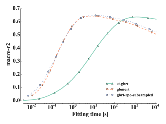
(a) Friedman1-chain

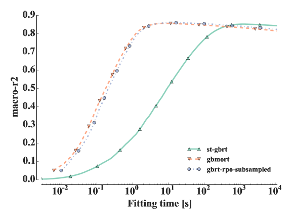
(b) Friedman1-group

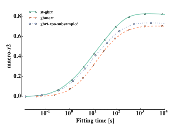
(c) Friedman1-ind

Figure 1: The convergence speed and the optimum reached are affected by the output correlation structure. The gbmort and gbrt-rpo-subsampled algorithms both exploit output correlations, which yields faster convergence and slightly better performance than st-gbrt on friedman1-chain and friedman1-group. However, st-gbrt converges to a better optimum than gbmort and gbrt-rpo-subsample when there is no output correlation as in friedman1-ind. (Model parameters: $k=p$, $n_{\max{}\_leaves}=2$, $\mu=0.1$)

On the friedman1-chain (see Figure 1a) and friedman1-group (see Figure 1b), gbmort and gbrt-rpo-subsampled converge more than 100 times faster (note the logarithmic scale of the abscissa) than single target. Furthermore, the optimal macro-$r^{2}$ is slightly better for gbmort and gbrt-rpo-subsampled than st-gbrt. All methods are over-fitting after a sufficient amount of time. Since all outputs are correlated on both datasets, gbmort and gbrt-rpo-susbsampled are exploiting the output structure to have faster convergence. The gbmort method exploits the output structure by filtering the output noise as the stump fitted at each iteration is the one that maximizes the reduction of the average output variance. By contrast, gbrt-rpo-subsample detects output correlations by optimizing the $\rho_{m}$ constant and then shares the information obtained by the current weak model with all other outputs.

On the friedman1-ind dataset (see Figure 1c), all three methods converge at the same rate. However, the single target strategy converges to a better optimum than gbmort and gbrt-rpo-subsample. Since all outputs are independent, single target enforces the proper correlation structure (see Figure 1c). The gbmort method has the worst performance as it assumes the wrong set of hypotheses. The gbrt-rpo-subsampled method pays the price of its flexibility by over-fitting the additive weight associated to each output, but less than gbmort.

This experiment confirms that enforcing the right correlation structure yields faster convergence and the best accuracy. Nevertheless, the output structure is unknown in practice. We need flexible approaches such as gbrt-rpo-subsampled that automatically detects and exploits the correlation structure.

4.2.3 Performance and output modeling assumption

The presence or absence of structures among the outputs has shown to affect the convergence speed of multi-output gradient boosting methods. As discussed in Dembczyński et al (2012), we talk about conditionally independent outputs when:

$$P(y_{1},\ldots,y_{q}|x)=P(y_{1}|x)\cdots P(y_{q}|x)$$

and about unconditionally independent outputs when:

$$P(y_{1},\ldots,y_{q})=P(y_{1})\cdots P(y_{q}).$$

When the outputs are not conditionally independent and the loss function can not be decomposed over the outputs (eg., the subset $0-1$ loss), one might need to model the joint output distribution $P(y_{1},\ldots,y_{q}|x)$ to obtain a Bayes optimal prediction. If the outputs are conditionally independent however or if the loss function can be decomposed over the outputs, then a Bayes optimal prediction can be obtained by modeling separately the marginal conditional output distributions $P(y_{j}|x)$ for all $j$. This suggests that in this case, binary relevance / single target is not really penalized asymptotically with respect to multiple output methods for not considering the outputs jointly. In the case of an infinite sample size, it is thus expected to provide as good models as all the multiple output methods. Since in practice we have to deal with finite sample sizes, multiple output methods may provide better results by better controlling the bias/variance trade-off.

Let us study this question on the three synthetic datasets: friedman1-chain, friedman1-group or friedman1-ind. We optimize the hyper-parameters with a computational budget of 10000 weak models per hyper-parameter set. Five strategies are compared (i) the artificial-gbrt method, which assumes that the output structure is known and implements the optimal strategy on each problem as explained in Section 4.2.1, (ii) single target of gradient boosting regression trees (st-gbrt), (iii) gradient boosting with multi-output regression tree (gbmort, Algorithm 2) and gradient boosting with randomly sub-sampled outputs (iv) without relabelling (gbrt-rpo-subsampled, Algorithm 3) and (v) with relabelling (gbrt-relabel-rpo-subsampled, Algorithm 4). All boosting algorithms minimize the square loss, the absolute loss or their multi-outputs extension the $\ell_{2}$-norm loss.

We give the performance on the three tasks for each estimator in Table 4 and the p-value of Student’s paired $t$-test comparing the performance of two estimators on the same dataset in Table 5.

Table 4: All methods compared on the 3 artificial datasets. Exploiting the output correlation structure (if it exists) allows beating single target in a finite sample size, decomposable metric and conditionally independent output.

Dataset	friedman1-chain	friedman1-group	friedman1-ind
artificial-gbrt	$0.654\pm 0.015$ (1)	$0.889\pm 0.009$ (1)	$0.831\pm 0.004$ (1)
st-gbrt	$0.626\pm 0.016$ (5)	$0.873\pm 0.008$ (5)	$0.830\pm 0.003$ (2)
gbmort	$0.640\pm 0.008$ (4)	$0.874\pm 0.012$ (4)	$0.644\pm 0.010$ (5)
gbrt-relabel-rpo-subsampled	$0.648\pm 0.015$ (2)	$0.880\pm 0.009$ (2)	$0.706\pm 0.009$ (4)
gbrt-rpo-subsampled	$0.645\pm 0.013$ (3)	$0.876\pm 0.007$ (3)	$0.789\pm 0.003$ (3)

Table 5: P-values given by Student’s paired $t$-test on the synthetic datasets. We highlight p-values inferior to $\alpha=0.05$ in bold. Note that the sign $>$ (resp. $<$) indicates that the estimator in the row has better (resp.lower) score than the column estimator.

	artificial-gbrt	st-gbrt	gbmort	gbrt-relabel-rpo-subsampled	gbrt-rpo-subsampled
Dataset friedman1-chain
artificial-gbrt		0.003(>)	0.16	0.34	0.24
st-gbrt	0.003(<)		0.11	0.04(<)	0.03(<)
gbmort	0.16	0.11		0.38	0.46
gbrt-relabel-rpo-subsampled	0.34	0.04(>)	0.38		0.57
gbrt-rpo-subsampled	0.24	0.03(>)	0.46	0.57
Dataset friedman1-group
artificial-gbrt		0.005(>)	0.009(>)	0.047(>)	0.006(>)
st-gbrt	0.005(<)		0.56	0.046(<)	0.17
gbmort	0.009(<)	0.56		0.15	0.63
gbrt-relabel-rpo-subsampled	0.047(<)	0.046(>)	0.15		0.04(>)
gbrt-rpo-subsampled	0.006(<)	0.17	0.63	0.04(<)
Dataset friedman1-ind
artificial-gbrt		0.17	2e-06(>)	2e-06(>)	1e-05(>)
st-gbrt	0.17		2e-06(>)	4e-06(>)	4e-06(>)
gbmort	2e-06(<)	2e-06(<)		9e-05(<)	6e-06(<)
gbrt-relabel-rpo-subsampled	2e-06(<)	4e-06(<)	9e-05(>)		3e-05(<)
gbrt-rpo-subsampled	1e-05(<)	4e-06(<)	6e-06(>)	3e-05(>)

As expected, we obtain the best performance if the output correlation structure is known with the custom strategies implemented with artificial-gbrt. Excluding this artificial method, the best boosting methods on the two problems with output correlations, friedman1-chain and friedman1-group, are the two gradient boosting approaches with output subsampling (gbrt-relabel-rpo-subsampled and gbrt-rpo-subsampled).

In friedman1-chain, the output correlation structure forms a chain as each new output is the previous one in the chain with a noisy output. Predicting outputs at the end of the chain, without using the previous ones, is a difficult task. The single target approach is thus expected to be sub-optimal. And indeed, on this problem, artificial-gbrt, gbrt-relabel-rpo-subsampled and gbrt-rpo-subsampled are significantly better than st-gbrt (with $\alpha=0.05$). All the multi-output methods, including gbmort, are indistinguishable from a statistical point of view, but we note that gbmort is however not significantly better than st-gbrt.

In friedman1-group, among the ten pairs of algorithms, four are not significantly different, showing a p-value greater than 0.05 (see Table 5). We first note that gbmort is not better than st-gbrt while exploiting the correlation. Secondly, the boosting methods with random output sub-sampling are the best methods. They are however not significantly better than gbmort and significantly worse than artificial-gbrt, which assumes the output structure is known. Note that gbrt-relabel-rpo-subsampled is significantly better than gbrt-rpo-subsampled.

In friedman1-ind, where there is no correlation between the outputs, the best strategy is single target which makes independent models for each output. From a conceptual and statistical point of view, there is no difference between artificial-gbrt and st-gbrt. The gbmort algorithm, which is optimal when all outputs are correlated, is here significantly worse than all other methods. The two boosting methods with output subsampling (gbrt-rpo-subsampled and gbrt-relabel-rpo-subsampled method), which can adapt themselves to the absence of correlation between the outputs, perform better than gbmort, but they are significantly worse than st-gbrt. For these two algorithms, we note that not relabelling the leaves (gbrt-rpo-subsampled) leads to superior performance than relabelling them (gbrt-relabel-rpo-subsampled). Since in friedman1-ind the outputs have disjoint feature support, the test nodes of a decision tree fitted on one output will partition the samples using these features. Thus, it is not suprising that relabelling the tree leaves actually deteriorates performance.

In the previous experiment, all the outputs were dependent of the inputs. However in multi-output tasks with very high number of outputs, it is likely that some of them have few or no links with the inputs, i.e., are pure noise. Let us repeat the previous experiments with the main difference that we add to the original 16 outputs 16 purely noisy outputs obtained through random permutations of the original outputs. We show the results of optimizing each algorithm in Table 6 and the associated p-values in Table 7. We report the macro-$r^{2}$ score computed either on all outputs (macro-$r^{2}$) including the noisy outputs or only on the 16 original outputs (half-macro-$r^{2}$). P-values were computed between each pair of algorithms using Student’s $t$-test on the macro $r^{2}$ score computed on all outputs.

We observe that the gbrt-rpo-subsampled algorithm has the best performance on friedman1-chain and friedman1-group and is the second best on the friedman1-ind, below st-gbrt. Interestingly on friedman1-chain and friedman1-group, this algorithm is significantly better than all the others, including gbmort. Since this latter method tries to fit all outputs simultaneously, it is the most disadvantaged by the introduction of the noisy outputs.

Table 6: Friedman datasets with noisy outputs.

friedman1-chain	half-macro-$r^{2}$	macro-$r^{2}$
st-gbrt	0.611 (4)	$0.265\pm 0.006$ (4)
gbmort	0.617 (3)	$0.291\pm 0.012$ (3)
gbrt-relabel-rpo-subsampled	0.628 (2)	$0.292\pm 0.006$ (2)
gbrt-rpo-subsampled	0.629 (1)	$0.303\pm 0.007$ (1)
Friedman1-group	half-macro-$r^{2}$	macro-$r^{2}$
st-gbrt	0.840 (3)	$0.364\pm 0.007$ (4)
gbmort	0.833 (4)	$0.394\pm 0.004$ (3)
gbrt-relabel-rpo-subsampled	0.855 (2)	$0.395\pm 0.005$ (2)
gbrt-rpo-subsampled	0.862 (1)	$0.414\pm 0.006$ (1)
Friedman1-ind	half-macro-$r^{2}$	macro-$r^{2}$
st-gbrt	0.806 (1)	$0.3536\pm 0.0015$ (1)
gbmort	0.486 (4)	$0.1850\pm 0.0081$ (4)
gbrt-relabel-rpo-subsampled	0.570 (3)	$0.2049\pm 0.0033$ (3)
gbrt-rpo-subsampled	0.739 (2)	$0.3033\pm 0.0021$ (2)

Table 7: P-values given by Student’s paired $t$-test on the synthetic datasets with additional noisy outputs. We highlight p-values inferior to $\alpha=0.05$ in bold. Note that the sign $>$ (resp. $<$) indicates that the estimator in the row has better (resp.lower) score than the column estimator.

	st-gbrt	gbmort	gbrt-relabel-rpo-subsampled	gbrt-rpo-subsampled
Dataset friedman1-chain
st-gbrt		0.0009(<)	0.0002(<)	0.0002(<)
gbmort	0.0009(>)		0.86	0.04(<)
gbrt-relabel-rpo-subsampled	0.0002(>)	0.86		0.03(<)
gbrt-rpo-subsampled	0.0002(>)	0.04(>)	0.03(>)
Dataset friedman1-group
st-gbrt		0.0002(<)	0.0006(<)	0.0003(<)
gbmort	0.0002(>)		0.74	0.008(<)
gbrt-relabel-rpo-subsampled	0.0006(>)	0.74		0.002(<)
gbrt-rpo-subsampled	0.0003(>)	0.008(>)	0.002(>)
Dataset friedman1-ind
st-gbrt		1e-06(>)	1e-07(>)	1e-06(>)
gbmort	1e-06(<)		0.02(<)	6e-06(<)
gbrt-relabel-rpo-subsampled	1e-07(<)	0.02(>)		2e-06(<)
gbrt-rpo-subsampled	1e-06(<)	6e-06(>)	2e-06(>)

4.3 Effect of random projection

With the gradient boosting and random projection of the output space approaches (Algorithms 3 and 4), we have considered until now only sub-sampling a single output at each iteration as random projection scheme. In Section 4.3.1, we show empirically the effect of other random projection schemes such as Gaussian random projection. In Section 4.3.2, we study the effect of increasing the number of projections in the gradient boosting algorithm with random projection of the output space and relabelling (parameter $q$ of Algorithm  4). We also show empirically the link between Algorithm  4 and gradient boosting with multi-output regression tree (Algorithm 2).

4.3.1 Choice of the random projection scheme

Beside random output sub-sampling, we can combine the multi-output gradient boosting strategies (Algorithms 3 and 4) with other random projection schemes. A key difference between random output sub-sampling and random projections such as Gaussian and (sparse) Rademacher projections is that the latter combines together several outputs.

We show in Figures 2, 3 and 4 the LRAP or macro-$r^{2}$ score convergence of gradient boosting with randomly projected outputs (gbrt-rpo, Algorithm 3) respectively on the mediamill, delicious, and Friedman1-ind datasets with different random projection schemes.

The impact of the random projection scheme on convergence speed of gbrt-rpo (Algorithm 3) is very problem dependent. On the mediamill dataset, Gaussian, Achlioptas, or sparse random projections all improve convergence speed by a factor of 10 (see Figure 2) compared to subsampling randomly only one output. On the delicious (Figure 3) and friedman1-ind (Figure 4), this is the opposite: subsampling leads to faster convergence than all other projections schemes. Note that we have the same behavior if one relabels the tree structure grown at each iteration as in Algorithm 4 (results not shown).

Dense random projections, such as Gaussian random projections, force the weak model to consider several outputs jointly and it should thus only improve when outputs are somewhat correlated (which seems to be the case on mediamill). When all of the outputs are independent or the correlation is less strong, as in friedman1-ind or delicious, this has a detrimental effect. In this situation, sub-sampling only one output at each iteration leads to the best performance.

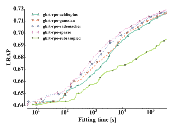
Figure 2: On the mediamill dataset, Gaussian, Achlioptas and sparse random projections with gbrt-rpo (Algorithm 3) show 10 times faster convergence in terms of LRAP score, than sub-sampling one output variable at each iteration. ($k=p$, stumps, $\mu=0.1$, logistic loss)

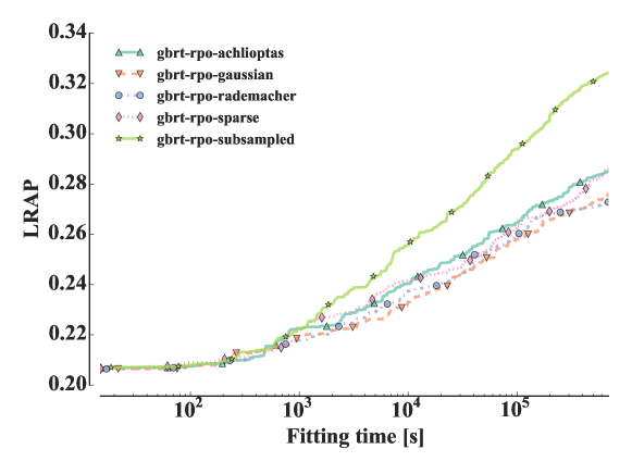
Figure 3: On the delicious dataset, Gaussian, Achlioptas and sparse random projections with gbrt-rpo (Algorithm 3) show 10 times faster convergence in terms of LRAP score, than sub-sampling one output variable at each iteration. ($k=p$, stumps, $\mu=0.1$, logistic loss)

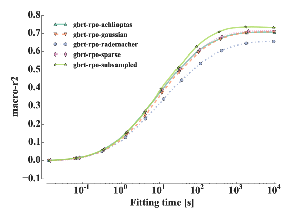
Figure 4: On the friedman1-ind dataset where there is no output correlation, gbrt-rpo (Algorithm 3) with one random subsampled output leads to a higher macro-$r^{2}$ score than using Gaussian, Achlioptas or sparse random projections. ($k=p$, stumps, $\mu=0.1$, square loss)

4.3.2 Effect of the size of the projected space

The multi-output gradient boosting strategy combining random projections and tree relabelling (Algorithm 4) can use more than one random projection ($q\geq 1$) by using multi-output trees as base learners. In this section, we study the effect of the size of the projected space $q$ in Algorithm 4. This approach corresponds to the one developed in Joly et al (2014) for random forest transposed to gradient boosting.

Figure 5 shows the LRAP score as a function of the fitting time for gbmort (Algorithm 2) and gbrt-relabel-rpo (Algorithm 4) with either Gaussian random projection (see Figure 5a) or output subsampling (see Figure 5b) for a number of projections $q\in\left\{1,98,196,491\right\}$ on the delicious dataset. In Figure 5a and Figure 5b, one Gaussian random projection or one sub-sampled output has faster convergence than their counterparts with a higher number of projections $q$ and gbmort at fixed computational budget. Note that when the number of projections $q$ increases, gradient boosting with random projection of the output space and relabelling becomes similar to gbmort.

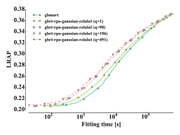
(a)

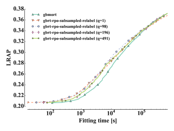
(b)

Figure 5: On the delicious dataset, LRAP score as a function of the boosting ensemble fitting time for gbrt-rpo-gaussian-relabel and gbrt-rpo-subsampled-relabel with different number of projections $q$. ($k=p$, stumps, $\mu=0.1$, logistic loss)

Instead of fixing the computational budget as a function of the training time, we now set the computational budget to 100 boosting steps. On the delicious dataset, gbrt-relabel-rpo (Algorithm 4) with Gaussian random projection yields approximately the same performance as gbmort with $q\geq 20$ random projections as shown in Figure 6a and reduces computing times by a factor of 7 at $q=20$ projections (see Figure 6b).

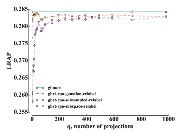
(a)

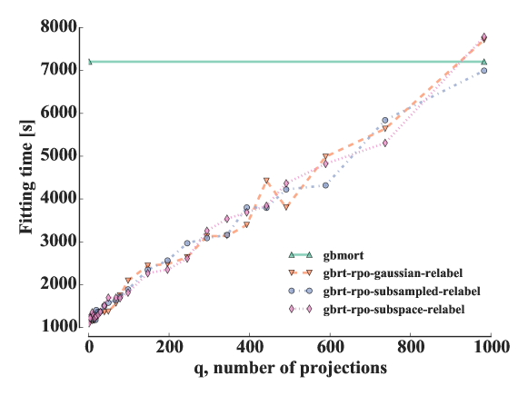
(b)

Figure 6: On delicious, increasing the number of random projections $q$ allows to reach the same LRAP score as gbmort at a significantly reduced computational cost. ($k=p$, stumps, $\mu=0.1$, $M=100$, logistic loss)

These experiments show that gradient boosting with random projection and relabelling (gbrt-relabel-rpo, Algorithm 4) is indeed an approximation of gradient boosting with multi-output trees (gbmort, Algorithm 2). The number of random projections $q$ influences simultaneously the bias-variance tradeoff and the convergence speed of Algorithm 4.

4.4 Systematic analysis over real world datasets

We perform a systematic analysis over real world multi-label classification and multi-output regression datasets. For this study, we evaluate the proposed algorithms: gradient boosting of multi-output regression trees (gbmort, Algorithm 2), gradient boosting with random projection of the output space (gbrt-rpo, Algorithm 3), and gradient boosting with random projection of the output space and relabelling (gbrt-relabel-rpo, Algorithm 4). For the two latter algorithms, we consider two random projection schemes: (i) Gaussian random projection, a dense random projection, and (ii) random output sub-sampling, a sparse random projection. They will be compared to three common and well established tree-based multi-output algorithms: (i) binary relevance / single target of gradient boosting regression tree (br-gbrt / st-gbrt), (ii) multi-output random forest (mo-rf) and (iii) binary relevance / single target of random forest models (br-rf / st-rf).

We will compare all methods on multi-label tasks in Section 4.4.1 and on multi-output regression tasks in Section 4.4.2. Following the recommendations in (Demšar, 2006), we use the Friedman test and its associated Nemenyi post-hoc test to assess the statistical significance of the observed differences. Pairwise comparisons are also carried out using the Wilcoxon signed ranked test.

4.4.1 Multi-label datasets

The critical distance diagram of Figure 7 gives the ranks of the algorithms over the 21 multi-label datasets and has an associated Friedman test p-value of $1.36\times 10^{-10}$ with a critical distance of $2.29$ given by the Nemenyi post-hoc test ($\alpha=0.05$). Thus, we can reject the null hypothesis that all methods are equivalent. Table 8 gives the outcome of the pairwise Wilcoxon signed ranked tests. Detailed scores are provided in Appendix D.

The best average performer is gbrt-relabel-rpo-gaussian which is significantly better according to the Nemenyi post-hoc test than all methods except gbrt-rpo-gaussian and gbmort.

Gradient boosting with the Gaussian random projection has a significantly better average rank than the random output sub-sampling projection. Relabelling tree leaves allows to have better performance on the 21 multi-label dataset. Indeed, both gbrt-relabel-rpo-gaussian and gbrt-relabel-rpo-subsampled are better ranked and significantly better than their counterparts without relabelling (gbrt-rpo-gaussian and gbrt-rpo-subsampled).

Among all compared methods, br-gbrt has the worst rank and it is significantly worse than all gbrt variants according to the Wilcoxon signed rank test. This might be actually a consequence of the constant budget in time that was allocated to all methods (see Section 4.1). All methods were given the same budget in time but, given the very slow convergence rate of br-gbrt, this budget may not allow to grow enough trees per output with this method to reach competitive performance.

We notice also that both random forests based methods (mo-rf and br-rf) are less good than all gbrt variants, most of the time significantly, except for br-gbrt. It has to be noted however that no hyper-parameter was tuned for the random forests. Such tuning could slightly change our conclusions, although random forests often work well with default setting.

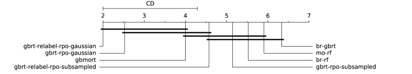
Figure 7: Critical difference diagram between algorithms on the multi-label datasets.

Table 8: P-values given by the Wilcoxon signed rank test on the multi-label datasets. We bold p-values below $\alpha=0.05$. Note that the sign $>$ (resp. $<$) indicates that the row estimator has superior (resp. inferior) LRAP score than the column estimator.

	br-gbrt	br-rf	gbmort	gbrt-relabel-rpo-gaussian	gbrt-relabel-rpo-subsampled	gbrt-rpo-gaussian	gbrt-rpo-subsampled	mo-rf
br-gbrt		0.79	0.001(<)	6e-05(<)	0.001(<)	0.0001(<)	0.003(<)	0.54
br-rf	0.79		0.01(<)	0.002(<)	0.02(<)	0.005(<)	0.07	0.29
gbmort	0.001(>)	0.01(>)		0.001(<)	0.36	0.04(<)	0.03(>)	0.02(>)
gbrt-relabel-rpo-gaussian	6e-05(>)	0.002(>)	0.001(>)		0.0002(>)	0.005(>)	7e-05(>)	0.0007(>)
gbrt-relabel-rpo-subsampled	0.001(>)	0.02(>)	0.36	0.0002(<)		0.0002(<)	0.02(>)	0.008(>)
gbrt-rpo-gaussian	0.0001(>)	0.005(>)	0.04(>)	0.005(<)	0.0002(>)		7e-05(>)	0.002(>)
gbrt-rpo-subsampled	0.003(>)	0.07	0.03(<)	7e-05(<)	0.02(<)	7e-05(<)		0.04(>)
mo-rf	0.54	0.29	0.02(<)	0.0007(<)	0.008(<)	0.002(<)	0.04(<)

4.4.2 Multi-output regression datasets

The critical distance diagram of Figure 8 gives the rank of each estimator over the 8 multi-output regression datasets. The associated Friedman test has a p-value of $0.3$. Given the outcome of the test, we can therefore not reject the null hypothesis that the estimator performances can not be distinguished. Table 9 gives the outcomes of the pairwise Wilcoxon signed ranked tests. They confirm the fact that all methods are very close to each other as only two comparisons show a p-value lower than 0.05 (st-rf is better than st-gbrt and gbrt-rpo-subsampled). This lack of statistical power is probably partly due here to the smaller number of datasets included in the comparison (8 problems versus 21 problems in classification and 8 methods tested over 8 problems). Please, see Appendix E for the detailed scores.

If we ignore statistical tests, as with multi-label tasks, gbrt-relabel-rpo-gaussian has the best average rank and st-gbrt the worst average rank. This time however, gbrt-relabel-rpo-gaussian is followed by the random forest based algorithms (st-rf and mo-rf) and gbmort. Given the lack of statistical significance, this ranking should however be intrepreted cautiously.

Figure 8: Critical difference diagram between algorithm on the multi-output regression datasets.

Table 9: P-value given by the Wilcoxon signed rank test on multi-output regression datasets. We bold p-values below $\alpha=0.05$. Note that the sign $>$ (resp. $<$) indicates that the row estimator has superior (resp. inferior) macro-$r^{2}$ score than the column estimator.

	st-gbrt	st-rf	gbmort	gbrt-relabel-rpo-gaussian	gbrt-relabel-rpo-subsampled	gbrt-rpo-gaussian	gbrt-rpo-subsampled	mo-rf
st-gbrt		0.02(<)	0.26	0.58	0.78	0.67	0.89	0.16
st-rf	0.02(>)		0.33	0.67	0.09	0.09	0.04(>)	0.58
gbmort	0.26	0.33		0.4	0.16	0.67	0.4	0.48
gbrt-relabel-rpo-gaussian	0.58	0.67	0.4		0.16	0.4	0.48	0.58
gbrt-relabel-rpo-subsampled	0.78	0.09	0.16	0.16		0.16	1	0.07
gbrt-rpo-gaussian	0.67	0.09	0.67	0.4	0.16		0.48	0.26
gbrt-rpo-subsampled	0.89	0.04(<)	0.4	0.48	1	0.48		0.4
mo-rf	0.16	0.58	0.48	0.58	0.07	0.26	0.4

5 Related works

Binary relevance Tsoumakas et al (2009) / single target Spyromitros-Xioufis et al (2012) is often suboptimal as it does not exploit potential correlations that might exist between the outputs. For this reason, several approaches have been proposed in the literature that improve over binary relevance by exploiting output dependencies. Besides the multi-output tree-based methods discussed in Sections 2.1 and 3.1, with which we compared ourself empirically in Section 4, we review in this section several other related algorithms relying either on random projection of the output space, explicit consideration of output dependencies, or on the sharing of models learnt for one output with the others. We refer the interested reader to Zhang and Zhou (2014); Tsoumakas et al (2009); Gibaja and Ventura (2014); Borchani et al (2015); Spyromitros-Xioufis et al (2012) for more complete reviews of multilabel/multi-output methods, and to Madjarov et al (2012) for an empirical comparison of these methods.

Given a specific multi-label or multi-output regression loss function, one can sometimes exploit its mathematical properties to derive a specific Adaboost algorithm: minimizing at each boosting step the selected loss function by choosing carefully the sample weights prior training a weak estimator. Each loss minimizable in such way ending with its own dedicated training algorithm: Adaboost.MH Schapire and Singer (1999) for the Hamming loss, Adaboost.MR for the Ranking loss Schapire and Singer (1999), Adaboost.LC for the covering loss Amit et al (2007), AdaBoostSeq Kajdanowicz and Kazienko (2013) for the sequence loss and Adaboost.MRT Kummer and Najjaran (2014) for the $\ell_{1}$ loss. By contrast as Friedman (2001), we have instead defined boosting algorithms applicable to the whole family of differentiable loss functions through a gradient descent inspired approach. Note that prior multi-output gradient boosting approach has also focused on either the $\ell_{2}$ loss Geurts et al (2007) or the covariance discrepancy loss Miller et al (2016).

Random projections have been exploited by several authors to solve multi-output supervised learning problems. Hsu et al (2009); Kapoor et al (2012) address sparse multi-label problems using compressed sensing techniques. The original output label vector is projected into a low dimensional space and then a (linear) regression model is fit on each projected output in the reduced space. At prediction time, the predictions made by all estimators are then concatenated and decoded back into the original space. This latter step requires to solve an inverse problem exploiting the sparsity of the original label vector. Tsoumakas et al (2014) also train single-output models (gradient boosted trees) independently on random linear projections of the output vector. Unlike Hsu et al (2009) however, the number of generated random projections is actually larger than the number of original outputs, since this is expected to improve accuracy by adding an ensemble effect, and decoding involves solving an overdetermined linear system, which can be done without requiring any sparsity assumption. In our own previous work Joly et al (2014), we investigated random output projections to fasten and improve the accuracy of multi-output random forests. Each tree of the forest is a multi-output tree which is fitted on a low-dimensional random projection of the original outputs, with the projection renewed for each tree independently. Tree leaves of the resulting forest are then relabeled in the original output space (as in Algorithm 4). With respect to Hsu et al (2009); Kapoor et al (2012); Tsoumakas et al (2014), relabelling the leaves avoids having to solve an inverse problem at prediction time, which improves computing times and also reduces the risk of introducing errors at decoding.

The previous approaches exploit the output correlation only implicitely in that the individual models are trained to fit random linear combinations incorporating each several outputs. Individual models are however trained independently of each other. In our approach, we take more explicitely output dependencies into account by iteratively fitting linearly the current random projection estimator to (the current residuals of) all outputs at each iteration. In this sense, our work is related to several multi-label or multi-target methods that try to more explicitely exploit output dependencies or to convey information from one output to the others. For example, in the estimator chain approach Read et al (2011); Dembczynski et al (2010); Spyromitros-Xioufis et al (2012), the conditional probability $P_{\mathcal{Y}|\mathcal{X}}(y|x)$ is modeled using the chain rule:

$$P_{\mathcal{Y}|\mathcal{X}}(y|x)=P_{\mathcal{Y}_{1}|\mathcal{X}}(y_{1}|x)\prod_{j=2}^{d}P_{\mathcal{Y}_{j}|\mathcal{X},\mathcal{Y}_{1},\ldots,\mathcal{Y}_{j-1}}(y_{j}|x,y_{1},\ldots,y_{j-1}).$$ (33)

The factors of this decomposition are learned in sequence, each one using the predictions of the previously learnt models as auxiliary inputs. Like our approach, these methods are thus also able to benefit from output dependencies to obtain simpler and/or better estimators. Several works have extended the estimator chain idea by exploiting other (data induced) factorization of the conditional output distribution, derived for example from a bayesian network structure Zhang and Zhang (2010) or using the composition property Gasse et al (2015).

Two works at least are based on the idea of sharing models trained for one output with the others (in the context of multi-label classification). Huang et al (2012) propose to generate an ensemble through a sequential approach: at each step, one model is fitted for each output independently without taking into account the others, and then an optimal linear combination of these models is fitted to each output so as to minimize the selected loss. The process is costly as one has to fit several linear models at each iteration. Convergence speed of this method with respect to the number of base models is also expected to be slower than ours, because information between outputs is shared less frequently (every $d$ base models, with $d$ the number of labels). Yan et al (2007) propose a two-step approach. First, a pool of models is generated by training a single individual classifier for each label independently (using feature randomization and bootstrapping). A boosted ensemble is then fit for each label independently using base models selected from the pool obtained during the first step (each one potentially trained for a label different from the targeted one). This approach is less adaptive than others since the pool of base models is fixed, for efficiency reasons.

Finally, more complementary to our work, Si et al (2017) recently proposed an efficient implementation of a multi-label gradient boosted decision tree method (very similar to the gbmort method studied here) for handling very high dimensional and sparse label vectors. While very effective, this implementation aims at improving prediction time and model size in the presence of sparse outputs and does not change the representation bias with respect to gbmort. It should thus suffer from the same limitations as this method in terms of predictive performance.

6 Conclusions

In this paper, we have first formally extended the gradient boosting algorithm to multi-output tasks leading to the “multi-output gradient boosting algorithm” (gbmort). It sequentially minimizes a multi-output loss using multi-output weak models considering that all outputs are correlated. By contrast, binary relevance / single target of gradient boosting models fits one gradient boosting model per output considering that all outputs are independent. However in practice, we do not expect to have either all outputs independent or all outputs dependent. So, we propose a more flexible approach which adapts automatically to the output correlation structure called “gradient boosting with random projection of the output space” (gbrt-rpo). At each boosting step, it fits a single weak model on a random projection of the output space and optimize a multiplicative weight separately for each output. We have also proposed a variant of this algorithm (gbrt-relabel-rpo) only valid with decision trees as weak models: it fits a decision tree on the randomly projected space and then it relabels tree leaves with predictions in the original (residual) output space. The combination of the gradient boosting algorithm and the random projection of the output space yields faster convergence by exploiting existing correlations between the outputs and by reducing the dimensionality of the output space. It also provides new bias-variance-convergence trade-off potentially allowing to improve performance.

We have evaluated in depth these new algorithms on several artificial and real datasets. Experiments on artificial problems highlighted that gb-rpo with output subsampling offers an interesting tradeoff between single target and multi-output gradient boosting. Because of its capacity to automatically adapt to the output space structure, it outperforms both methods in terms of convergence speed and accuracy when outputs are dependent and it is superior to gbmort (but not st-rt) when outputs are fully independent. On the 29 real datasets, gbrt-relabel-rpo with the denser Gaussian projections turns out to be the best overall approach on both multi-label classification and multi-output regression problems, although all methods are statistically undistinguisable on the regression tasks. Our experiments also show that gradient boosting based methods are competitive with random forests based methods. Given that multi-output random forests were shown to be competitive with several other multi-label approaches in Madjarov et al (2012), we are confident that our solutions will be globally competitive as well, although a broader empirical comparison should be conducted as future work. One drawback of gradient boosting with respect to random forests however is that its performance is more sensitive to its hyper-parameters that thus require careful tuning. Although not discussed in this paper, besides predictive performance, gbrt-rpo (without relabeling) has also the advantage of reducing model size with respect to mo-rf (multi-output random forests) and gbmort, in particular in the presence of many outputs. Indeed, in mo-rf and gbmort, one needs to store a vector of the size of the number of outputs per leaf node. In gbrt-rpo, one needs to store only one real number (a prediction for the projection) per leaf node and a vector of the size of the number of outputs per tree ($\rho_{m}$). At fixed number of trees and fixed tree complexity, this could lead to a strong reduction of the model memory requirement when the number of labels is large. Note that the approach proposed in Joly et al (2014) does not solve this issue because of leaf node relabeling. This could be addressed by deactivating leaf relabeling and inverting the projection at prediction time to obtain a prediction in the original output space, as done for example in Hsu et al (2009); Kapoor et al (2012); Tsoumakas et al (2014). However, this would be at the expense of computing times at prediction time and of accuracy because of the potential introduction of errors at the decoding stage. Finally, while we restricted our experiments here to tree-based weak learners, Algorithms 2 and 3 are generic and could exploit respectively any multiple output and any single output regression method. As future work, we believe that it would interesting to evaluate them with other weak learners.

7 Acknowledgements

Part of this research has been done while A. Joly was a research fellow of the FNRS, Belgium. This work is partially supported by the IUAP DYSCO, initiated by the Belgian State, Science Policy Office.

Appendix A Convergence when $M\rightarrow\infty$

Similarly to Geurts et al (2007), we can prove the convergence of the training-set loss of the gradient boosting with multi-output models (Algorithm 2), and gradient boosting on randomly projected spaces with (Algorithm 3) or without relabelling (Algorithm 4).

Since the loss function is lower-bounded by $0$, we merely need to show that the loss $\ell$ is non-increasing on the training set at each step $m$ of the gradient boosting algorithm.

For Algorithm 2 and Algorithm 4, we note that

$$\sum_{i=1}^{n}\ell(y^{i},f_{m}(x^{i})) =\min_{\rho\in\mathbb{R}^{d}}\sum_{i=1}^{n}\ell\left(y^{i},f_{m-1}(x^{i})+\rho\odot g_{m}(x^{i})\right)$$

$$\leq\sum_{i=1}^{n}\ell\left(y^{i},f_{m-1}(x^{i})\right).$$ (34)

and the learning-set loss is hence non increasing with $M$ if we use a learning rate $\mu=1$. If the loss $\ell(y,y^{\prime})$ is convex in its second argument $y^{\prime}$ (which is the case for those loss-functions that we use in practice), then this convergence property actually holds for any value $\mu\in(0;1]$ of the learning rate. Indeed, we have

$$\sum_{i=1}^{n}\ell\left(y^{i},f_{m-1}(x^{i})\right)$$

$$\geq (1-\mu)\sum_{i=1}^{n}\ell\left(y^{i},f_{m-1}(x^{i})\right)+\mu\sum_{i=1}^{n}\ell\left(y^{i},f_{m-1}(x^{i})+\rho_{m}\odot g_{m}(x^{i})\right)$$

$$\geq \sum_{i=1}^{n}\ell\left(y^{i},f_{m-1}(x^{i})+\mu\rho_{m}\odot g_{m}(x^{i})\right).$$

given Equation 34 and the convexity property.

For Algorithm 3, we have a weak estimator $g_{m}$ fitted on a single random projection of the output space $\phi_{m}$ with a multiplying constant vector $\rho_{m}\in\mathbb{R}^{d}$, and we have:

$$\sum_{i=1}^{n}\ell(y^{i},f_{m}(x^{i})) =\min_{\rho\in\mathbb{R}^{d}}\sum_{i=1}^{n}\ell\left(y^{i},f_{m-1}(x^{i})+\rho g_{m}(x^{i})\right)$$

$$\leq\sum_{i=1}^{n}\ell\left(y^{i},f_{m-1}(x^{i})\right).$$ (35)

and the error is also non increasing for Algorithm 3, under the same conditions as above.

The previous development shows that Algorithm 2, Algorithm 3 and Algorithm 4 are converging on the training set for a given loss $\ell$. The binary relevance / single target of gradient boosting regression trees admits a similar convergence proof. We expect however the convergence speed of the binary relevance / single target to be lower assuming that it fits one weak estimator for each output in a round robin fashion.

Appendix B Representation bias of decision tree ensembles

Random forests and gradient tree boosting build an ensemble of trees either independently or sequentially, and thus offer different bias/variance tradeoffs. The predictions of all these ensembles can be expressed as a weighted combination of the ground truth outputs of the training set samples. In the present section, we discuss the differences between single tree models, random forest models and gradient tree boosting models in terms of the representation biases of the obtained models. We also highlight the differences between single target models and multi-output tree models.

Single tree models.

The prediction of a regression tree learner can be written as a weighted linear combination of the training samples $\mathcal{L}=\{(x^{i},y^{i})\in\mathcal{X}\times\mathcal{Y}\}_{i=1}^{n}$. We associate to each training sample $(x^{i},y^{i})$ a weight function $w^{i}:\mathcal{X}\rightarrow\mathbb{R}$ which gives the contribution of a ground truth $y^{i}$ to predict an unseen sample $x$. The prediction of a single output tree $f$ is given by

$$f(x)=\sum_{i=1}^{n}w^{i}(x)y^{i}.$$ (36)

The weight function $w^{i}(x)$ is non zero if both the samples $(x^{i},y^{i})$ and the unseen sample $x$ reach the same leaf of the tree. If both $(x^{i},y^{i})$ and $x$ end up in the same leaf of the tree, $w^{i}(x)$ is equal to the inverse of the number of training samples reaching that leaf. The weight $w^{i}(x)$ can thus be rewritten as $k(x^{i},x)$ and the function $k(\cdot,\cdot)$ is actually a positive semi-definite kernel Geurts et al (2006).

We can also express multi-output models as a weighted sum of the training samples. With a single target regression tree, we have an independent weight function $w^{i}_{j}$ for each sample $i$ of the training set and each output $j$ as we fit one model per output. The prediction of this model for output $j$ is given by:

$$f(x)_{j}=\sum_{i=1}^{n}w^{i}_{j}(x)y^{i}_{j}.$$ (37)

With a multi-output regression tree, the decision tree structure is shared between all outputs so we have a single weight function $w^{i}$ for each training sample $i$:

$$f(x)_{j}=\sum_{i=1}^{n}w^{i}(x)y^{i}_{j}.$$ (38)

Random forest models.

If we have a single target random forest model, the prediction of the $j$-th output combines the predictions of the $M$ models of the ensemble in the following way:

$$f(x)_{j}=\frac{1}{M}\sum_{m=1}^{M}\sum_{i=1}^{n}w^{i}_{m,j}(x)y^{i}_{j},$$ (39)

with one weight function $w^{i}_{m,j}$ per tree, sample and output. We note that we can combine the weights of the individual trees into a single weight per sample and per output

$$w^{i}_{j}(x)=\frac{1}{M}\sum_{m=1}^{M}w^{i}_{m,j}(x).$$ (40)

The prediction of the $j$-th output for an ensemble of independent models has thus the same form as a single target regression tree model:

$$f(x)_{j}=\frac{1}{M}\sum_{m=1}^{M}\sum_{i=1}^{n}w^{i}_{m,j}(x)y^{i}_{j}=\sum_{i=1}^{n}w^{i}_{j}(x)y^{i}_{j}.$$ (41)

We can repeat the previous development with a multi-output random forest model. The prediction for the $j$-th output of an unseen sample $x$ combines the predictions of the $M$ trees:

$$f(x)_{j} =\frac{1}{M}\sum_{m=1}^{M}\sum_{i=1}^{n}w^{i}_{m}(x)y^{i}_{j}=\sum_{i=1}^{n}w^{i}(x)y^{i}_{j}$$ (42)

with

$$w^{i}(x)=\frac{1}{M}\sum_{m=1}^{M}w^{i}_{m}(x).$$ (43)

With this framework, the prediction of an ensemble model has the same form as the prediction of a single constituting tree.

Gradient tree boosting models.

The prediction of a single output gradient boosting tree ensemble is given by

$$f(x)=\rho_{0}+\sum_{m=1}^{M}\mu\rho_{m}g_{m}(x),$$ (44)

but also as

$$f(x)=\sum_{m=1}^{M}\sum_{i=1}^{n}w^{i}_{m}(x)y^{i}=\sum_{i=1}^{n}w^{i}(x)y^{i},$$ (45)

where the weight $w^{i}(x)$ takes into account the learning rate $\mu$, the prediction of all tree models $g_{m}$ and the associated $\rho_{m}$. Given the similarity between gradient boosting prediction and random forest model, we deduce that the single target gradient boosting tree ensemble has the form of Equation 37 and that multi-output gradient tree boosting (Algorithm 2) and gradient boosting tree with projection of the output space and relabelling (Algorithm 4) has the form of Equation 38.

However, we note that the prediction model of the gradient tree boosting with random projection of the output space (Algorithm 3) is not given by Equation 37 and Equation 38 as the prediction of a single output $j$ can combine the predictions of all $d$ outputs. More formally, the prediction of the $j$-th output is given by:

$$f(x)_{j}=\sum_{m=1}^{M}\sum_{i=1}^{n}\sum_{k=1}^{d}w^{i}_{m,j,k}(x)y^{i}_{k},$$ (46)

where the weight function $w^{i}_{m,j,k}$ takes into account the contribution of the $m$-th model fitted on a random projection $\phi_{m}$ of the output space to predict the $j$-th output using the $k$-th outputs and the $i$-th sample. The triple summation can be simplified by using a single weight to summarize the contribution of all $M$ models:

$$f(x)_{j} =\sum_{m=1}^{M}\sum_{i=1}^{n}\sum_{k=1}^{d}w^{i}_{m,j,k}(x)y^{i}_{k}=\sum_{i=1}^{n}\sum_{k=1}^{d}w^{i}_{j,k}(x)y^{i}_{k}.$$ (47)

Between the studied methods, we can distinguish three groups of multi-output tree models. The first one considers that all outputs are independent as with binary relevance / single target trees, random forests or gradient tree boosting models. The second group with multi-output random forests, gradient boosting of multi-output tree and gradient boosting with random projection of the output space and relabelling share the tree structures between all outputs, but the leaf predictions are different for each output. The last and most flexible group is the gradient tree boosting with random projection of the output space sharing both the tree structures and the leaf predictions. We will highlight in the experiments the impact of these differences in representation biases.

Appendix C Real world datasets

Experiments are performed on several multi-label datasets: the yeast Elisseeff and Weston (2001) and the bird Briggs et al (2013) datasets in the biology domain; the corel5k Duygulu et al (2002) and the scene Boutell et al (2004) datasets in the image domain; the emotions Tsoumakas et al (2008b) and the CAL500 Turnbull et al (2008) datasets in the music domain; the bibtex Katakis et al (2008), the bookmarks Katakis et al (2008), the delicious Tsoumakas et al (2008a), the enron Klimt and Yang (2004), the genbase Diplaris et al (2005), and the medical datasets in the text domain and the mediamill Snoek et al (2006) dataset in the video domain.

Several hierarchical classification tasks are also included to increase the diversity in the number of labels. They are treated as flat multi-label classification tasks, with each node of the hierarchy treated as one label. Nodes of the hierarchy which never occured in the training and testing set were removed. The reuters Rousu et al (2005), WIPO Rousu et al (2005) datasets are from the text domain. The Diatoms Dimitrovski et al (2012) dataset is from the image domain. SCOP-GO Clare (2003), Yeast-GO Barutcuoglu et al (2006) and Expression-GO Vens et al (2008) are from the biological domain. Missing values in the Expression-GO dataset were inferred using the median for continuous features and the most frequent value for categorical features using the entire dataset. The inference of a drug-protein interaction network Yamanishi et al (2011) is also considered either using the drugs to infer the interactions with the protein (drug-interaction), either using the proteins to infer the interactions with the drugs (protein-interaction).

Multi-output regression approaches are evaluated on several real world datasets: the edm Karalič and Bratko (1997) dataset in the industrial domain; the water-quality Džeroski et al (2000) dataset in the environmental domain; the atp1d Spyromitros-Xioufis et al (2012), the atp7d Spyromitros-Xioufis et al (2012), the scm1d Spyromitros-Xioufis et al (2012) and the scm20d Spyromitros-Xioufis et al (2012) datasets in the price prediction domain; the oes97 Spyromitros-Xioufis et al (2012) and the oes10 Spyromitros-Xioufis et al (2012) datasets in the human resource domain. All outputs in these datasets were normalized to have zero mean and unit variance.

Appendix D Performance of tree ensemble models over the multi-label datasets

Table 10 and Table 11 show the performance of the random forest models and the boosting algorithms over the 21 multi-label datasets.

Table 10: LRAP scores over 21 multi-label datasets (part 1).

	CAL500	bibtex	birds
br-gbrt	$0.505\pm 0.002$ (3.5)	$0.587\pm 0.007$ (6)	$0.787\pm 0.009$ (6)
br-rf	$0.484\pm 0.002$ (8)	$0.542\pm 0.005$ (8)	$0.802\pm 0.013$ (1)
gbmort	$0.501\pm 0.005$ (6)	$0.595\pm 0.005$ (4.5)	$0.772\pm 0.007$ (8)
gbrt-relabel-rpo-gaussian	$0.507\pm 0.009$ (1)	$0.607\pm 0.005$ (1)	$0.800\pm 0.017$ (2)
gbrt-relabel-rpo-subsampled	$0.499\pm 0.008$ (7)	$0.596\pm 0.005$ (3)	$0.790\pm 0.016$ (4)
gbrt-rpo-gaussian	$0.505\pm 0.006$ (3.5)	$0.600\pm 0.003$ (2)	$0.793\pm 0.017$ (3)
gbrt-rpo-subsampled	$0.506\pm 0.006$ (2)	$0.595\pm 0.007$ (4.5)	$0.779\pm 0.018$ (7)
mo-rf	$0.502\pm 0.003$ (5)	$0.553\pm 0.005$ (7)	$0.789\pm 0.012$ (5)
	bookmarks	corel5k	delicious
br-gbrt	$0.4463\pm 0.0038$ (7)	$0.291\pm 0.006$ (7)	$0.347\pm 0.002$ (8)
br-rf	$0.4472\pm 0.0019$ (6)	$0.273\pm 0.012$ (8)	$0.373\pm 0.004$ (6.5)
gbmort	$0.4855\pm 0.0016$ (2)	$0.312\pm 0.009$ (3.5)	$0.384\pm 0.003$ (3.5)
gbrt-relabel-rpo-gaussian	$0.4893\pm 0.0003$ (1)	$0.315\pm 0.007$ (1.5)	$0.389\pm 0.003$ (1)
gbrt-relabel-rpo-subsampled	$0.4718\pm 0.0034$ (4)	$0.310\pm 0.007$ (5)	$0.384\pm 0.003$ (3.5)
gbrt-rpo-gaussian	$0.4753\pm 0.0022$ (3)	$0.315\pm 0.010$ (1.5)	$0.386\pm 0.004$ (2)
gbrt-rpo-subsampled	$0.4621\pm 0.0026$ (5)	$0.312\pm 0.006$ (3.5)	$0.377\pm 0.003$ (5)
mo-rf	$0.4312\pm 0.0023$ (8)	$0.294\pm 0.010$ (6)	$0.373\pm 0.004$ (6.5)
	diatoms	drug-interaction	emotions
br-gbrt	$0.623\pm 0.007$ (7.5)	$0.271\pm 0.018$ (8)	$0.800\pm 0.022$ (7)
br-rf	$0.623\pm 0.011$ (7.5)	$0.310\pm 0.009$ (5)	$0.816\pm 0.009$ (1)
gbmort	$0.656\pm 0.012$ (4)	$0.304\pm 0.005$ (7)	$0.794\pm 0.014$ (8)
gbrt-relabel-rpo-gaussian	$0.725\pm 0.010$ (1)	$0.326\pm 0.008$ (1)	$0.802\pm 0.017$ (5.5)
gbrt-relabel-rpo-subsampled	$0.685\pm 0.012$ (3)	$0.322\pm 0.009$ (3)	$0.808\pm 0.021$ (3)
gbrt-rpo-gaussian	$0.702\pm 0.014$ (2)	$0.323\pm 0.011$ (2)	$0.804\pm 0.009$ (4)
gbrt-rpo-subsampled	$0.653\pm 0.013$ (5.5)	$0.312\pm 0.013$ (4)	$0.802\pm 0.007$ (5.5)
mo-rf	$0.653\pm 0.010$ (5.5)	$0.308\pm 0.007$ (6)	$0.810\pm 0.010$ (2)
	enron	genbase	mediamill
br-gbrt	$0.685\pm 0.006$ (6)	$0.989\pm 0.009$ (8)	$0.7449\pm 0.0020$ (8)
br-rf	$0.683\pm 0.005$ (7)	$0.994\pm 0.005$ (2)	$0.7819\pm 0.0009$ (1)
gbmort	$0.705\pm 0.004$ (2.5)	$0.990\pm 0.004$ (6)	$0.7504\pm 0.0013$ (7)
gbrt-relabel-rpo-gaussian	$0.705\pm 0.003$ (2.5)	$0.993\pm 0.006$ (3)	$0.7660\pm 0.0021$ (3)
gbrt-relabel-rpo-subsampled	$0.697\pm 0.004$ (5)	$0.990\pm 0.010$ (6)	$0.7588\pm 0.0013$ (5)
gbrt-rpo-gaussian	$0.706\pm 0.004$ (1)	$0.992\pm 0.007$ (4)	$0.7608\pm 0.0008$ (4)
gbrt-rpo-subsampled	$0.699\pm 0.005$ (4)	$0.990\pm 0.005$ (6)	$0.7519\pm 0.0006$ (6)
mo-rf	$0.676\pm 0.004$ (8)	$0.995\pm 0.004$ (1)	$0.7793\pm 0.0015$ (2)

Table 11: LRAP scores over 21 multi-label datasets (part 2).

	medical	protein-interaction	reuters
br-gbrt	$0.864\pm 0.006$ (3)	$0.294\pm 0.007$ (6)	$0.939\pm 0.0033$ (7)
br-rf	$0.821\pm 0.007$ (8)	$0.293\pm 0.006$ (7)	$0.9406\pm 0.0016$ (6)
gbmort	$0.867\pm 0.011$ (1.5)	$0.310\pm 0.007$ (2.5)	$0.9483\pm 0.0014$ (3)
gbrt-relabel-rpo-gaussian	$0.867\pm 0.019$ (1.5)	$0.310\pm 0.009$ (2.5)	$0.9508\pm 0.0009$ (1)
gbrt-relabel-rpo-subsampled	$0.856\pm 0.012$ (5)	$0.303\pm 0.003$ (4.5)	$0.9441\pm 0.0016$ (4)
gbrt-rpo-gaussian	$0.859\pm 0.017$ (4)	$0.311\pm 0.007$ (1)	$0.9486\pm 0.0021$ (2)
gbrt-rpo-subsampled	$0.851\pm 0.009$ (6)	$0.303\pm 0.003$ (4.5)	$0.9430\pm 0.0031$ (5)
mo-rf	$0.827\pm 0.006$ (7)	$0.288\pm 0.009$ (8)	$0.9337\pm 0.0021$ (8)
	scene	scop-go	sequence-funcat
br-gbrt	$0.880\pm 0.003$ (4)	$0.716\pm 0.047$ (8)	$0.678\pm 0.008$ (6)
br-rf	$0.876\pm 0.003$ (6)	$0.798\pm 0.004$ (2)	$0.658\pm 0.008$ (7)
gbmort	$0.886\pm 0.004$ (1)	$0.796\pm 0.007$ (3)	$0.699\pm 0.005$ (3)
gbrt-relabel-rpo-gaussian	$0.884\pm 0.006$ (2.5)	$0.788\pm 0.006$ (4)	$0.703\pm 0.007$ (2)
gbrt-relabel-rpo-subsampled	$0.879\pm 0.008$ (5)	$0.770\pm 0.010$ (6)	$0.685\pm 0.008$ (5)
gbrt-rpo-gaussian	$0.884\pm 0.005$ (2.5)	$0.775\pm 0.018$ (5)	$0.706\pm 0.007$ (1)
gbrt-rpo-subsampled	$0.875\pm 0.006$ (7)	$0.723\pm 0.016$ (7)	$0.691\pm 0.006$ (4)
mo-rf	$0.865\pm 0.003$ (8)	$0.800\pm 0.006$ (1)	$0.643\pm 0.003$ (8)
	wipo	yeast	yeast-go
br-gbrt	$0.706\pm 0.009$ (6)	$0.756\pm 0.009$ (8)	$0.499\pm 0.009$ (4.5)
br-rf	$0.633\pm 0.013$ (7)	$0.760\pm 0.008$ (3.5)	$0.463\pm 0.010$ (7)
gbmort	$0.762\pm 0.011$ (3)	$0.760\pm 0.007$ (3.5)	$0.504\pm 0.015$ (3)
gbrt-relabel-rpo-gaussian	$0.776\pm 0.012$ (1)	$0.762\pm 0.007$ (2)	$0.524\pm 0.012$ (1)
gbrt-relabel-rpo-subsampled	$0.751\pm 0.017$ (4)	$0.758\pm 0.005$ (5.5)	$0.496\pm 0.013$ (6)
gbrt-rpo-gaussian	$0.763\pm 0.010$ (2)	$0.763\pm 0.005$ (1)	$0.522\pm 0.012$ (2)
gbrt-rpo-subsampled	$0.724\pm 0.011$ (5)	$0.758\pm 0.008$ (5.5)	$0.499\pm 0.011$ (4.5)
mo-rf	$0.624\pm 0.018$ (8)	$0.757\pm 0.008$ (7)	$0.415\pm 0.014$ (8)

Appendix E Performance of tree ensemble models over the multi-output regression datasets

Table 12 shows the performance of the random forest models and the boosting algorithms over the 8 multi-output regression datasets.

Table 12: Performance over 8 multi-output regression dataset

	atp1d	atp7d	edm
gbmort	$0.80\pm 0.03$ (5.5)	$0.63\pm 0.03$ (2)	$0.39\pm 0.16$ (3)
gbrt-relabel-rpo-gaussian	$0.81\pm 0.03$ (3.5)	$0.66\pm 0.04$ (1)	$0.25\pm 0.28$ (8)
gbrt-relabel-rpo-subsampled	$0.79\pm 0.04$ (7)	$0.54\pm 0.13$ (7)	$0.35\pm 0.10$ (5)
gbrt-rpo-gaussian	$0.80\pm 0.04$ (5.5)	$0.54\pm 0.20$ (7)	$0.36\pm 0.04$ (4)
gbrt-rpo-subsampled	$0.81\pm 0.04$ (3.5)	$0.54\pm 0.16$ (7)	$0.31\pm 0.27$ (7)
mo-rf	$0.82\pm 0.03$ (2)	$0.60\pm 0.06$ (4)	$0.51\pm 0.02$ (1)
st-gbrt	$0.78\pm 0.05$ (8)	$0.59\pm 0.08$ (5)	$0.34\pm 0.14$ (6)
st-rf	$0.83\pm 0.02$ (1)	$0.61\pm 0.07$ (3)	$0.47\pm 0.04$ (2)
	oes10	oes97	scm1d
gbmort	$0.77\pm 0.05$ (3.5)	$0.67\pm 0.07$ (8)	$0.908\pm 0.003$ (4.5)
gbrt-relabel-rpo-gaussian	$0.75\pm 0.04$ (7.5)	$0.71\pm 0.07$ (2.5)	$0.910\pm 0.004$ (2.5)
gbrt-relabel-rpo-subsampled	$0.75\pm 0.06$ (7.5)	$0.68\pm 0.07$ (6)	$0.912\pm 0.003$ (1)
gbrt-rpo-gaussian	$0.77\pm 0.03$ (3.5)	$0.68\pm 0.08$ (6)	$0.910\pm 0.004$ (2.5)
gbrt-rpo-subsampled	$0.76\pm 0.02$ (5.5)	$0.71\pm 0.08$ (2.5)	$0.908\pm 0.004$ (4.5)
mo-rf	$0.76\pm 0.04$ (5.5)	$0.69\pm 0.05$ (4)	$0.898\pm 0.004$ (8)
st-gbrt	$0.79\pm 0.03$ (1.5)	$0.68\pm 0.07$ (6)	$0.905\pm 0.003$ (7)
st-rf	$0.79\pm 0.03$ (1.5)	$0.72\pm 0.05$ (1)	$0.907\pm 0.004$ (6)
	scm20d	water-quality
gbmort	$0.856\pm 0.006$ (2)	$0.14\pm 0.01$ (4.5)
gbrt-relabel-rpo-gaussian	$0.862\pm 0.006$ (1)	$0.15\pm 0.01$ (2)
gbrt-relabel-rpo-subsampled	$0.854\pm 0.007$ (3)	$0.14\pm 0.02$ (4.5)
gbrt-rpo-gaussian	$0.852\pm 0.006$ (4)	$0.14\pm 0.01$ (4.5)
gbrt-rpo-subsampled	$0.850\pm 0.007$ (5)	$0.13\pm 0.02$ (7.5)
mo-rf	$0.849\pm 0.007$ (6.5)	$0.16\pm 0.01$ (1)
st-gbrt	$0.836\pm 0.006$ (8)	$0.13\pm 0.02$ (7.5)
st-rf	$0.849\pm 0.006$ (6.5)	$0.14\pm 0.01$ (4.5)

References

- Achlioptas (2003) Achlioptas D (2003) Database-friendly random projections: Johnson-lindenstrauss with binary coins. Journal of computer and System Sciences 66(4):671–687
- Agrawal et al (2013) Agrawal R, Gupta A, Prabhu Y, Varma M (2013) Multi-label learning with millions of labels: Recommending advertiser bid phrases for web pages. In: Proceedings of the 22nd international conference on World Wide Web, International World Wide Web Conferences Steering Committee, pp 13–24
- Amit et al (2007) Amit Y, Dekel O, Singer Y (2007) A boosting algorithm for label covering in multilabel problems. In: Artificial Intelligence and Statistics, pp 27–34
- Barutcuoglu et al (2006) Barutcuoglu Z, Schapire RE, Troyanskaya OG (2006) Hierarchical multi-label prediction of gene function. Bioinformatics 22(7):830–836
- Blockeel et al (2000) Blockeel H, De Raedt L, Ramon J (2000) Top-down induction of clustering trees. arXiv preprint cs/0011032
- Borchani et al (2015) Borchani H, Varando G, Bielza C, Larrañaga P (2015) A survey on multi-output regression. Wiley Interdisciplinary Reviews: Data Mining and Knowledge Discovery 5(5):216–233
- Boutell et al (2004) Boutell MR, Luo J, Shen X, Brown CM (2004) Learning multi-label scene classification. Pattern recognition 37(9):1757–1771
- Breiman (2001) Breiman L (2001) Random forests. Machine learning 45(1):5–32
- Breiman et al (1984) Breiman L, Friedman J, Stone CJ, Olshen RA (1984) Classification and regression trees. CRC press
- Brent (2013) Brent RP (2013) Algorithms for minimization without derivatives. Courier Corporation
- Briggs et al (2013) Briggs F, Huang Y, Raich R, Eftaxias K, Lei Z, Cukierski W, Hadley SF, Hadley A, Betts M, Fern XZ, et al (2013) The 9th annual mlsp competition: New methods for acoustic classification of multiple simultaneous bird species in a noisy environment. In: Machine Learning for Signal Processing (MLSP), 2013 IEEE International Workshop on, IEEE, pp 1–8
- Buitinck et al (2013) Buitinck L, Louppe G, Blondel M, Pedregosa F, Mueller A, Grisel O, Niculae V, Prettenhofer P, Gramfort A, Grobler J, et al (2013) Api design for machine learning software: experiences from the scikit-learn project. arXiv preprint arXiv:13090238
- Candes and Plan (2011) Candes EJ, Plan Y (2011) A probabilistic and ripless theory of compressed sensing. Information Theory, IEEE Transactions on 57(11):7235–7254
- Clare (2003) Clare A (2003) Machine learning and data mining for yeast functional genomics. PhD thesis, The University of Wales
- Dekel and Shamir (2010) Dekel O, Shamir O (2010) Multiclass-multilabel classification with more classes than examples. In: International Conference on Artificial Intelligence and Statistics, pp 137–144
- Dembczynski et al (2010) Dembczynski K, Cheng W, Hüllermeier E (2010) Bayes optimal multilabel classification via probabilistic classifier chains. In: ICML, vol 10, pp 279–286
- Dembczyński et al (2012) Dembczyński K, Waegeman W, Cheng W, Hüllermeier E (2012) On label dependence and loss minimization in multi-label classification. Machine Learning 88(1-2):5–45
- Demšar (2006) Demšar J (2006) Statistical comparisons of classifiers over multiple data sets. Journal of Machine learning research 7(Jan):1–30
- Dimitrovski et al (2012) Dimitrovski I, Kocev D, Loskovska S, Džeroski S (2012) Hierarchical classification of diatom images using ensembles of predictive clustering trees. Ecological Informatics 7(1):19–29
- Diplaris et al (2005) Diplaris S, Tsoumakas G, Mitkas PA, Vlahavas I (2005) Protein classification with multiple algorithms. In: Advances in Informatics, Springer, pp 448–456
- Duygulu et al (2002) Duygulu P, Barnard K, de Freitas JF, Forsyth DA (2002) Object recognition as machine translation: Learning a lexicon for a fixed image vocabulary. In: Computer Vision—ECCV 2002, Springer, pp 97–112
- Džeroski et al (2000) Džeroski S, Demšar D, Grbović J (2000) Predicting chemical parameters of river water quality from bioindicator data. Applied Intelligence 13(1):7–17
- Elisseeff and Weston (2001) Elisseeff A, Weston J (2001) A kernel method for multi-labelled classification. In: Advances in neural information processing systems, pp 681–687
- Freund and Schapire (1997) Freund Y, Schapire RE (1997) A decision-theoretic generalization of on-line learning and an application to boosting. Journal of computer and system sciences 55(1):119–139
- Friedman (1991) Friedman J (1991) Multivariate adaptive regression splines. The Annals of Statistics pp 1–67
- Friedman (2001) Friedman JH (2001) Greedy function approximation: a gradient boosting machine. Annals of statistics pp 1189–1232
- Friedman (2002) Friedman JH (2002) Stochastic gradient boosting. Computational Statistics & Data Analysis 38(4):367–378
- Gasse et al (2015) Gasse M, Aussem A, Elghazel H (2015) On the optimality of multi-label classification under subset zero-one loss for distributions satisfying the composition property. In: Proceedings of the 32nd International Conference on Machine Learning (ICML-15), pp 2531–2539
- Geurts et al (2006) Geurts P, Ernst D, Wehenkel L (2006) Extremely randomized trees. Machine learning 63(1):3–42
- Geurts et al (2007) Geurts P, Wehenkel L, d’Alché Buc F (2007) Gradient boosting for kernelized output spaces. In: Proceedings of the 24th international conference on Machine learning, ACM, pp 289–296
- Gibaja and Ventura (2014) Gibaja E, Ventura S (2014) Multi-label learning: a review of the state of the art and ongoing research. Wiley Interdisciplinary Reviews: Data Mining and Knowledge Discovery 4(6):411–444
- Haider et al (2015) Haider S, Rahman R, Ghosh S, Pal R (2015) A copula based approach for design of multivariate random forests for drug sensitivity prediction. PloS one 10(12):e0144,490
- Hastie et al (2005) Hastie T, Tibshirani R, Friedman J, Franklin J (2005) The elements of statistical learning: data mining, inference and prediction. The Mathematical Intelligencer 27(2):83–85
- Hsu et al (2009) Hsu D, Kakade S, Langford J, Zhang T (2009) Multi-label prediction via compressed sensing. In: NIPS, vol 22, pp 772–780
- Huang et al (2012) Huang SJ, Yu Y, Zhou ZH (2012) Multi-label hypothesis reuse. In: Proceedings of the 18th ACM SIGKDD international conference on Knowledge discovery and data mining, ACM, pp 525–533