On the measurements of assembly bias and splashback radius using optically selected galaxy clusters

Abstract

We critically examine the methodology behind the claimed observational detection of halo assembly bias using optically selected galaxy clusters by Miyatake et al. (2016) and More et al. (2016). We mimic the optical cluster detection algorithm and apply it to two different mock catalogs generated from the Millennium simulation galaxy catalog, one in which halo assembly bias signal is present, while the other in which the assembly bias signal has been expressly erased. We split each of these cluster samples into two using the average cluster-centric distance of the member galaxies to measure the difference in the clustering strength of the subsamples with respect to each other. We observe that the subsamples split by cluster-centric radii show differences in clustering strength, even in the catalog where the true assembly bias signal was erased. We show that this is a result of contamination of the member galaxy sample from interlopers along the line-of-sight. This undoubtedly shows that the particular methodology adopted in the previous studies cannot be used to claim a detection of the assembly bias signal. We figure out the tell-tale signatures of such contamination, and show that the observational data also shows similar signatures. Furthermore, we also show that projection effects in optical galaxy clusters can bias the inference of the 3-dimensional edges of galaxy clusters (splashback radius), so appropriate care should be taken while interpreting the splashback radius of optical clusters.

1 Introduction

In the $\Lambda$CDM paradigm, massive dark matter halos that host clusters of galaxies form at rare peaks of the initial density field. Such dark matter halos are biased tracers of the matter density and are more clustered than the underlying dark matter distribution itself. The clustering of dark matter halos primarily depends on halo mass (e.g Kaiser (1984); Efstathiou et al. (1988); Mo & White (1996)). However, there have been several studies which show that the clustering of halos at fixed mass can depend upon secondary properties such as the formation time and the concentration of halos (e.g Gao et al. (2005); Wechsler et al. (2006); Gao & White (2007); Faltenbacher & White (2010); Dalal et al. (2008)). This dependence of the halo clustering amplitude on secondary properties related to their assembly history other than the mass is commonly referred to as halo assembly bias.

Even though halo assembly bias is a well-known phenomenon in simulations and has been studied extensively, observational detection of halo assembly bias has been difficult and controversial (e.g Yang et al. (2006); Wang et al. (2013); Lin et al. (2016)). Recently, Miyatake et al. (2016) claimed evidence of halo assembly bias on galaxy cluster scales. They split the optically selected redMaPPer galaxy cluster catalog, using the compactness of member galaxies in the clusters as a proxy of halo concentration. Using weak gravitational lensing, they confirmed that the halo masses of these cluster subsamples were consistent with each other and yet the clustering amplitudes were significantly different. The difference in the clustering amplitude of the two subsamples was almost $60\%$, much larger than the difference expected from N-body simulations.

In a follow-up study, More et al. (2016) used the cross-correlation function of the same cluster subsamples with photometric SDSS galaxies to confirm the difference in the clustering amplitude of these subsamples with an enhanced signal-to-noise ratio. Additionally, More et al. (2016) measured the location of the splashback radius for these cluster subsamples. The splashback radius is the location of the first turn-around of the particles and is considered as a physical boundary of halos. The splashback radius depends on the accretion rates of halos (e.g., Diemer & Kravtsov (2014a); More et al. (2015a)). More et al. (2016) found that the low-concentration cluster subsample had a larger splashback radius than the high-concentration cluster subsample. Curiously, the inferred location of the splashback radius was smaller than that expected from numerical simulations.

There were two studies which critically examined the works by Miyatake et al. (2016) and More et al. (2016). Zu et al. (2017) examined whether the difference in the clustering amplitudes of the two cluster subsamples arose from biases in the cluster-centric radius due to projection effects. They proposed to use only those member galaxies which have high membership probabilities in order to define the cluster-centric average radius of member galaxies in order to reduce the contamination from projection effects. They showed that when such a radius is used to define the cluster subsamples, the clustering difference is reduced to levels which make it consistent or smaller than the maximum halo assembly bias signals seen in simulations.

However, one caveat in this analysis is that using only high probability members limits the use of the galaxy members which are closer to the cluster center, due to the way the redMaPPer algorithm assigns membership probabilities. It can be seen in numerical simulations that the assembly bias signal reduces in strength if the concentration derived from subhalos at a smaller radii is used to subdivide clusters at fixed halo mass in order to measure the assembly bias signal. Thus it is unclear if the reduced assembly bias signal seen in observations when using the new proxy is a result of such a selection or only a result of a reduction in projection effects.

In the second study, Busch & White (2017) mimicked the optical cluster finding algorithm in photometric imaging data on mock catalogs to investigate whether the large clustering difference in the two subsamples claimed in Miyatake et al. (2016) is consistent with $\Lambda$CDM. Their results showed that they could reproduce the observed clustering difference in the two subsamples seen in observations. The presence of projection effects in optical cluster catalogs was key to establishing the size of the signal observed. Although the seemingly large clustering difference could be reproduced in mock catalogs from $\Lambda$CDM, it remains unclear if the methodology used by Miyatake et al. (2016) and More et al. (2016) can be unambiguously used to detect halo assembly bias.

Addressing this question is the the central motivation of this paper. In order to carry out this investigation, we mimic the redMaPPer cluster finding algorithm closely and apply it to two different galaxy catalogs, one catalog which has assembly bias signal and the other one where the existing assembly bias has been artificially erased. If both the catalogs show an assembly bias signal following the analysis strategy adopted by Miyatake et al. (2016) and More et al. (2016), that would indicate that their methodology cannot be used to confirm or deny the existence of the assembly bias signal.

This paper is organized in the following manner. In Section 2, we describe the publicly available simulation data as well as the observational data we use in our analysis. Section 3 presents the simplified algorithm we use in order to mimic optical cluster finding in photometric data, our estimation of the compactness of galaxy clusters as a proxy of concentration of halos, steps to generate the catalog without assembly bias, and computation of correlation functions used in this paper. We presents our primary results in Section 4 and conclude in Section 5.

2 Data

2.1 Millennium Simulation: galaxy catalogs

We use the Millennium Simulation (Springel et al. (2005)), a $2160^{3}$ particle cosmological N-body simulation of a flat $\Lambda$CDM universe with box size of $500h^{-1}{\rm Mpc}$ and mass resolution of $8.6\times 10^{8}h^{-1}M_{\odot}$. The cosmological parameters used in this simulation are the matter density parameter $\Omega_{{\rm m}}=0.25$, the baryon density parameter $\Omega_{{\rm b}}=0.045$, the spectral index of initial density fluctuation $n_{\rm s}=1$, their amplitude specified by $\sigma_{8}=0.9$, and ${\rm H_{0}=73{\rm km}{\rm s^{-1}}{\rm Mpc^{-1}}}$. Haloes and their self-bound subhaloes were identified using the subfind algorithm (Springel et al. (2001)). The particular galaxy population used in this paper was created using the semi-analytic model for galaxy formation described in detail in Guo et al. (2011). In this paper, we use the same threshold as in Busch & White (2017) to select galaxies from a snapshot at $z=0.24$. We restrict ourselves to galaxies with $i$-band absolute magnitude $M_{i}<-20.14$ and with the specific star formation rate (SSFR) below $1.5\times 10^{-11}h{\rm yr}^{-1}$. The chosen magnitude limit is very close to the one corresponding to the redMaPPer luminosity limit of $0.2L_{\star}$ at $z=0.24$ (see Rykoff et al. (2012)), and the cut in the SSFR of the galaxies define a class of red galaxies. This selection criterion gives us $925114$ galaxies.

2.2 redMaPPer galaxy clusters

In order to compare our simulation based results to observations in the real Universe, we will make use of the redMaPPer galaxy cluster catalog. Using the imaging data processed in the Sloan Digital Sky Survey Data release 8 (Aihara (2011)), Rykoff et al. (2014) ran the red-sequence cluster finder, redMaPPer (Rykoff et al. (2014); Rozo & Rykoff (2014); Rozo et al. (2015a, b)), in order to find galaxy clusters. The galaxy clusters identified by redMaPPer have been assigned richness as well as redshifts. In order to mimic the selection criteria in More et al. (2016), we choose galaxy clusters with richness $20\leq\lambda\leq 100$ and redshifts between $0.1<z<0.33$. More than $80\%$ of galaxy clusters in the catalog have a spectroscopic redshift. We remove the remaining clusters which do not have a spectroscopic redshift from our analysis. We also use the random catalogs provided along with the redMaPPer cluster catalog. These catalogs contain corresponding position information, redshift, richness as well as a weight for each random cluster.

2.3 BOSS DR12 LOWZ sample

We will carry out a cross-correlation of the redMaPPer galaxy clusters with spectroscopic galaxies in order to study halo assembly bias. We use the spectroscopic galaxies in the large scale structure catalogs constructed from SDSS DR12 (Alam et al. (2015)). In particular we will use the LOWZ sample, since it has a large overlap in redshift range as our galaxy cluster sample. We restrict ourselves to LOWZ galaxies with redshifts between $0.1<z<0.33$, the same redshift range as our galaxy clusters. The galaxy catalogs also come with associated random galaxy catalogs that we use in order to perform our cross-correlation analysis.

3 Methods

The goal of this paper is to test the suitability of the methodology adopted by Miyatake et al. (2016) and More et al. (2016) to detect the assembly bias signal. As stated in the introduction, Busch & White (2017) showed that the large clustering difference observed by Miyatake et al. (2016) and More et al. (2016) in their cluster subsamples divided by $\langle R_{\rm mem}\rangle$ can be reproduced by running an analogue of the redMaPPer algorithm on mock galaxy catalogs. However, it is not clear whether the methodology used by Miyatake et al. (2016) and More et al. (2016) can unambiguously be used to detect halo assembly bias. Therefore to test this, we create a galaxy catalog where we erase the inherent assembly bias signal explicitly. We do this by exchanging the cluster-centric positions of galaxies in halos of the same mass. We call such galaxy catalogs “shuffled”.

We also implement an analogue of redMaPPer algorithm and apply it to both the original (hereafter, non-shuffled) and the shuffled catalogs. We will compare the difference of clustering amplitude from the shuffled catalogs with that obtained from the non-shuffled catalogs. In this section, we first describe our implementation of redMaPPer algorithm and the shuffled catalogs in Sec. 3.1 and 3.2 respectively, and then we discuss how we measure assembly bias signals and splashback radius in Sec. 3.3.

3.1 redMaPPer algorithm for mock catalogs

We implement a cluster identification algorithm based on the redMaPPer algorithm (Rykoff et al. (2014))using the projected distribution of galaxies. The algorithm uses multi-wavelength imaging data and identifies overdensities of red galaxies. The red galaxy spectrum shows a drop in their flux downward of 4000 Angstrom. This break moves through the different optical wavelength bands for galaxies with varying redshifts. In the absence of spectroscopic redshifts, this photometric feature helps to distinguish galaxies at different redshifts occupying the same position in the sky.

Ideally the redMaPPer algorithm can be directly applied to mock galaxy catalogs if the colors of galaxies are realistic. Unfortunately, redMaPPer has not been run on semi-analytical models due to either the non availability of light cone data or due to difficulties in reproducing the widths of the red sequence of galaxies in such models, which is critical for the identification of clusters (E. Rozo, E. Rykoff, priv. comm.). We make the simplifying assumption that the photometric redshift filter used to group galaxies along the redshift direction will have a poor resolution and therefore identify galaxies within a certain distance along the LOS as cluster members. These projection effects are expected to cause a systematic bias in the measurement of cluster observables. The effective LOS distance within which we consider galaxies as members of the cluster, will be called the projection length of the selection cylinder, or projection length in short.

We will vary the value of this projection length to assess its impact on our conclusions as well as to compare with the actual data.

Our algorithm is an improved version of the simplistic implementation of Busch & White (2017). In particular our algorithm will also assigns a membership probability $p_{{\rm mem}}$ to each galaxy in a manner similar to redMaPPer.

3.1.1 Algorithm

In redMaPPer, the probability that any galaxy found near a cluster center is part of the cluster with richness $\lambda$ is denoted by $p_{\rm mem}$ and is given by

$$p_{\rm mem}=\frac{\lambda u(x|\lambda)}{\lambda u(x|\lambda)+b(x)}\,,$$ (1)

where $x$ denotes properties of galaxies and includes the projected cluster-centric distance of the galaxy, $u(x|\lambda)$ denotes the normalized projected density profile of the galaxy cluster, and $b(x)$ denotes the background contamination. The total richness of a galaxy cluster should satisfy

$$\lambda=\sum_{R<R_{\rm c}(\lambda)}p_{\rm free}p_{\rm mem}(x|\lambda)\,,$$ (2)

where the sum goes over all members of a galaxy cluster within a cluster-centric radius $R<R_{\rm c}(\lambda)$ and the line-of-sight separation $|\pi|<d_{\rm cyl}^{\rm max}$. The probability $p_{\rm free}$ indicates the prior that the galaxy does not belong to any other richer galaxy cluster. The radial cut scales with $\lambda$ such that

$$R_{\rm c}(\lambda)=R_{0}(\lambda/100.0)^{\beta}\,,$$ (3)

where $R_{0}=1.0h^{-1}{\rm Mpc}$ and $\beta=0.2$ as adopted in redMaPPer. We will use three different values of $d_{\rm cyl}^{\rm max}$ ranging from $60h^{-1}{\rm Mpc}$ to $250h^{-1}{\rm Mpc}$ in our analysis.

The profile $u(x|\lambda)$ is the projected NFW profile (Navarro et al., 1997; Bartelmann, 1996) and is truncated smoothly at a projected radius $R=R_{\rm c}$ with an error function as described in Rykoff et al. (2014). The background $b(x)$ is assumed to be a constant to model the uncorrelated galaxies in the foreground and the background.

At first, all the galaxies in the catalog are considered potential cluster central galaxies and are given a probability $p_{\rm free}=1$ to be part of any cluster. We start our percolation of galaxy clusters by rank ordering galaxies by their stellar mass. We compute richness $\lambda$ for each candidate central galaxy by taking all the galaxies within a radius of $0.5h^{-1}{\rm Mpc}$ and $|\pi|<d_{\rm cyl}^{\rm max}$. In this first step, the membership probability for all galaxies is set to be unity if it is within the above defined cylinder. The probability $p_{\rm free}$ of each galaxy within this cylinder is then updated to be $p_{\rm free}=0$. The percolation steps continue by going down the rank ordered list of galaxy centers and ignoring those which have been assigned a $p_{\rm free}=0$. The purpose of this first step is to find an overall over-density regions which potentially have clusters. We eliminate all the candidates with $\lambda<3$ from the list.

Then, we reset $p_{\rm free}=1$ for all galaxies. We rank-order the clusters in a descending order based on the preliminary richness $\lambda$ and take percolation steps iteratively. Note that we simplify the rank-ordering by only using $\lambda$, while the actual redMaPPer algorithm implemented in Rykoff et al. (2014) rank ordered cluster center candidates by $\lambda$ as well as the $r$-band absolute magnitude of the galaxies. Starting from richest cluster, we take the following steps.

1. Given the $i^{\rm th}$ cluster in the list, recompute $\lambda$ and the membership probability based on the hitherto percolated galaxy catalog.

2. Determine the cluster center and clustering probability by numerically solving for Eq. 2. Take all the galaxies within the radius of $R_{c}(\lambda)$ and the projection length $\Delta\pi$. If there is a brighter galaxy than the current cluster center galaxy, consider the brightest one as a new center.

3. Recompute $\lambda$ with respect to the new central galaxy based on Eqs. 1 and 2.

4. Update the probability $p_{\rm free}$ for each galaxy to be $p_{\rm free}(1-p_{\rm mem})$ based on their membership probabilities of the current cluster. If $p_{\rm free}>0.5$, then these galaxies are eliminated from the list.

5. Repeat the steps for the next galaxy cluster in the ranked list.

Note that we model the photometric redshift uncertainty by using various projection lengths. To see whether the modeling of the projection affects our results, we also tried some window functions along the line-of-sight to model photometric redshift uncertainties in a slightly different manner, but we did not see significant changes in our results.

3.1.2 Definition of Concentration $R_{{\rm mem}}$

As a probe of cluster concentration measured from the distribution of member galaxies in clusters, Miyatake et al. (2016) and More et al. (2016) use the mean projected length of membership galaxies from the cluster center, $\langle R_{\rm mem}\rangle$ defined as

$$\langle R_{\rm mem}\rangle=\frac{\Sigma p_{{\rm mem},i}R_{{\rm mem},i}}{\Sigma p_{{\rm mem},i}},$$ (4)

where $p_{{\rm mem},i}$ and $R_{{\rm mem},i}$ are the membership probability and the projected distance from the cluster center of the $i$th member of galaxies in the cluster. As concentration has some dependencies on halo mass, $\langle R_{\rm mem}\rangle$ depends on redshift and richness $\lambda$, which is a proxy for cluster mass. In order to measure the assembly bias signals, we need to split the cluster sample into two subsamples with the same mass and which have different $\langle R_{\rm mem}\rangle$. To do this, we use 10 equally spaced bins both in redshift and λ and obtain the median of $\langle R_{\rm mem}\rangle$ as a function of redshift and $\lambda$. We then refer to clusters with $\langle R_{\rm mem}\rangle<\overline{\langle R_{\rm mem}\rangle}(z,\lambda)$ as “small-$\langle R_{\rm mem}\rangle$ clusters” and clusters with $<R_{{\rm mem}}>>\overline{\langle R_{\rm mem}\rangle}(z,\lambda)$ as “large-$<R_{{\rm mem}}>$ clusters”. This ensures that the two cluster subsamples have the same richness, and yet different internal structure. In order to mimic the methodology in Miyatake et al. (2016) and More et al. (2016), we use all the member galaxies including those with low membership probabilities.

3.2 Shuffled Catalogs

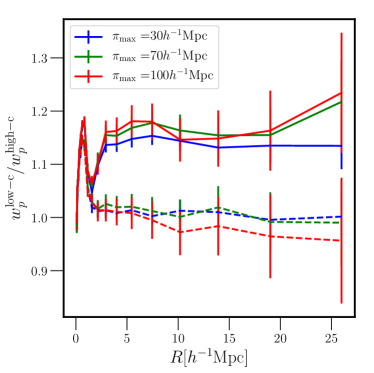
Figure 1: The figure shows our method of erasing assembly bias explicitly by using shuffled catalogs. Ratio of cluster-subhalo cross correlation functions between galaxy clusters with high and low dark matter concentration from the MultiDark Planck simulation at $z=0.25$. Each line corresponds to different integration scale $\pi_{\rm max}$. The solid lines correspond to the ratios measured from the non-shuffled catalogs, while the dashed lines are from the shuffled catalogs. Since the secondary parameter dependence is erased in the shuffled catalogs, we do not see any assembly biases from the shuffled catalogs.

Halo bias primarily depends on halo mass. However, halo bias depends on additional properties beyond their mass due to different assembly history of halos. This additional dependence of halo bias is called assembly bias. Since assembly bias is a secondary dependence of halo bias, we can erase the assembly bias from the catalog by shuffling the positions of the same mass halos. To do so, we first rank order halos by mass and split them into a series of bins with constant halo mass range. We use 10 bins, but the choice of the number of bins is arbitrary. For each mass bin, we shuffle the central positions of the host halos while maintaining the positions of the subhalos within their parent halos.

For demonstration purposes, we use halo catalogs from Multi-Dark Planck (MDPL) simulation (Klypin et al. (2016)) and select cluster-sized halos (i.e., $M_{\rm halo}>10^{14}h^{-1}{\rm M}_{\odot}$) splitting into low/high-concentration subsamples, where concentration is measured from dark matter profiles. Fig. 1 shows the ratio of projected correlation functions of low-concentration halos divided by those of high-concentration samples for several different integral scale along the line-of-sight. The catalogs with assembly bias (i.e., non-shuffled catalogs) exhibit the expected size of assembly bias signal for cluster-sized halos, while the subsamples from the shuffled catalogs do not show any bias differences. We choose several different maximum projection length $R=10h^{-1}{\rm Mpc}$ , $30h^{-1}{\rm Mpc}$, and $100h^{-1}{\rm Mpc}$ to compute projected correlation functions defined in Eq. 5. Bias ratios from both catalogs show little dependence on the integral scales.

Fig. 1 shows that the shuffled catalogs do not exhibit the assembly bias signals as expected. If the projected correlation functions of the redMaPPer clusters using the shuffled and the non-shuffled catalogs exhibit the similar result as Fig. 1, it implies that the assembly bias signals detected by Miyatake et al. (2016) and More et al. (2016) is actually a manifestation of assembly bias.

3.3 Correlation functions

We compute the projected cross-correlation functions for each cluster sample and the galaxy sample as

$$w_{p}(R)=\int_{0}^{\pi_{\rm max}}dr_{\pi}\xi_{gc}(R,r_{\pi}),$$ (5)

where $\pi_{\rm max}$ is the maximum integral scale, $\xi_{gc}$ is a two-dimensional cross correlation functions between clusters and galaxies. We use several different integral scales $\pi_{\rm max}$ to evaluate the contamination from the foreground/background galaxies. Busch & White (2017) and Zu et al. (2017) argued that the proxy of the concentration $\langle R_{\rm mem}\rangle$ is strongly affected by projection effects and therefore the parameter is correlated with the surrounding density field. We explicitly evaluate the level of contamination due to the projection effects by varying the integral scale $\pi_{\rm max}$. We use 102 jackknife regions in order to compute the error in the measurements of $w_{p}(R,r_{\pi}<\pi_{\rm max})$. The typical size of each of these jackknife patches is about $10\times 10$ square degrees, which corresponds to roughly $100\times 100(h^{-1}{\rm Mpc})^{2}$ for our cluster and galaxy samples. If the signal of assembly bias is purely due to foreground/background galaxies, we expect to see a dependence on the size of signal when varying $\pi_{\rm max}$.

3.4 Comparison with Observational Data

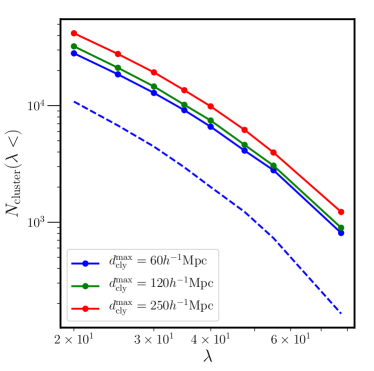
Figure 2: The number of clusters as a function of richness $\lambda$. Different colors correspond to the projection used to identify clusters. The dashed line corresponds to the number of clusters identified by redMaPPer from DR8.

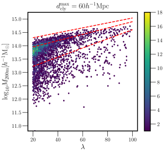
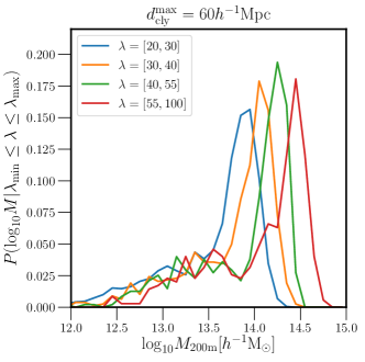
Figure 3: (Left) Comparison of galaxy clusters found using our mock redMaPPer method compared to inferences from real redMaPPer clusters. The left hand panel shows the halo mass-richness relation of the clusters selected using $d_{\rm cyl}^{\rm max}=60h^{-1}{\rm Mpc}$. The red dashed lines are the mean and standard deviation from Murata et al. (2018). The right hand panel shows the histograms of halo mass for different richness bins.

In this section, we compare properties of clusters identified by our analogue of redMaPPer and weak lensing analysis using redMaPPer clusters by Murata et al. (2018) to make sure that our version of redMaPPer can produce salient features of the observations. In Fig. 2, we plot a cumulative number of clusters in $(1h^{-1}{\rm Gpc})^{3}$ as a function of $\lambda$.

The solid lines with different colors show the result of running our mock redMaPPer algorithm on the Millennium galaxy catalog with different projection lengths to account for the uncertainties along the line-of-sight, while the dashed line shows the number of redMaPPer clusters in the original DR12 galaxy catalog. More number of clusters are identified by using longer projection lengths. This is because the number of member galaxies in the cylinder increases as the projection lengths and even slightly over-dense region can be identified as a cluster. This trend was also noted by Busch & White (2017). The figure also shows that our implementation of redMaPPer can reproduce the relative trend in the cluster number consistent with observations. Note that our comparison with the observations here can only be qualitative rather than quantitative. This partially stems from the fact that cosmological parameters used in the Millennium simulations are different from the Planck cosmology. In particular, due to the large value of $\sigma_{8}$ used in the Millennium simulations, the number of clusters can be about $25\%$ larger than that for the Planck cosmology at fixed halo mass (Busch & White (2017)). In addition, any differences between the mapping between colors of galaxies and their star formation rate cuts that we have used on the Millennium galaxy catalog to select our members, can cause systematic differences in richness and result in a larger number of galaxy clusters at a fixed richness. It is likely that our input galaxy catalog contains more number of galaxies, which causes the increase in the number of clusters and the decrease in the mean halo masses (see Fig. 3 ) at the fixed richness.

Next, we compare the richness-mass relation of the clusters identified from the Millennium simulation and the constraints from the weak lensing analysis of redMaPPer clusters carried out by Murata et al. (2018). The left panel of Fig. 3 shows the overall mass-richness relation of the clusters. The red dashed lines show the median and the 16th and 84th percentiles of the mass distribution for the redMaPPer clusters with $20\leq\lambda\leq 100$ as found by Murata et al. (2018). The scatter plot shows the halo mass richness relation of clusters identified in our mock run on the Millennium simulation. Our optical clusters also capture the same features as the observed mass-richness relation. The right panel shows the distribution of halo mass as a function of richness, which is also consistent with Murata et al. (2018) including the extended low-mass tail observed at fixed richness. This low-mass tail is due to the projection effects that the clusters contain some foreground/background galaxies and therefore these low-mass halos gain large enough richness.

4 Results

In this section, we present our findings regarding the use of optically selected clusters for measuring halo assembly bias as well as the splashback radius. We reiterate that our goals are two-fold: can we use the methodology adopted by Miyatake et al. (2016) and More et al. (2016) to (i) detect halo assembly bias (ii) or obtain an unbiased measurement of the splashback radius of optically selected galaxy clusters?

4.1 Halo assembly bias

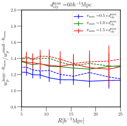
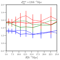
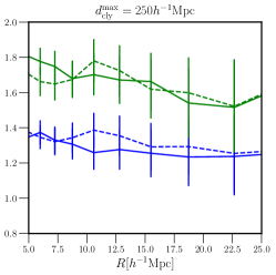
Figure 4: Dependence of the ratio of the projected correlation functions of the large/small-$<R_{\rm mem}>$ subsamples with different integral scales $\pi_{\rm max}$. From left to right panels correspond to the cluster samples with the projection lengths $d_{\rm cyl}^{\rm max}$ of $60$, $120$, and $250h^{-1}{\rm Mpc}$. Note that the projected correlation functions are computed in redshift-space.

We first present the results for halo assembly bias. We apply the algorithm described in Section 3.1 to the galaxy catalog from the Millennium simulation to select analogs of optically selected galaxy clusters. The one free parameter in our algorithm is the effective cylinder length $d_{\rm cyl}^{\rm max}$, galaxies within which get clubbed together in a single observationally identified galaxy clusters. Therefore we will show results for three different effective cylinder lengths, $d_{\rm cly}^{\rm max}=60h^{-1}{\rm Mpc}$, $120h^{-1}{\rm Mpc}$, and $250h^{-1}{\rm Mpc}$. The three panels of Fig. 4 show the ratio of the projected cross-correlation functions between galaxies and the subsamples of optically selected galaxy clusters identified by the three different effective cylinder lengths. We split the cluster samples into the large/small-$<R_{\rm mem}>$ subsamples, where $<R_{\rm mem}>$ is a proxy of concentration used in Miyatake et al. (2016) and More et al. (2016).

In each panel, the solid lines correspond to the ratio of the cross-correlation functions between the large/small-$<R_{\rm mem}>$ cluster subsamples from the non-shuffled catalogs. Unlike Miyatake et al. (2016), we have integrated the correlation function out to various integral scales, $\pi_{\rm max}=0.5\times d_{\rm cyl}^{\rm max}$, $d_{\rm cyl}^{\rm max}$, and $1.5\times d_{\rm cyl}^{\rm max}$. Note that for the case of $d_{\rm cyl}^{\rm max}=250h^{-1}{\rm Mpc}$, we cannot integrate out to $1.5\times d_{\rm cyl}^{\rm max}$ because the box size of the Millennium simulation is $500h^{-1}{\rm Mpc}$. We see that there is an apparent halo assembly bias signal seen in all three panels, where the small-$\langle R_{\rm mem}\rangle$ samples of galaxy clusters have a higher clustering signal on large scales compared to the large-$\langle R_{\rm mem}\rangle$ sample. The qualitative behaviour is very similar to that found by Miyatake et al. (2016) and More et al. (2016).

To ascertain that the difference in the clustering of the galaxy clusters is indeed a result of halo assembly bias, we now rerun the same measurements, but now by selecting clusters from a galaxy catalog where halo assembly bias was intentionally erased (i.e., shuffled catalogs). If the difference in clustering that we see is indeed due to halo assembly bias, then the difference in the clustering signal should vanish in this null test as with Fig. 1. The resulting cross-correlation functions of the clusters and galaxies in the shuffled galaxy catalogs are shown as dashed lines in Fig. 4. We observe that within the error bars of our measurement, we see consistent levels of differences in the clustering amplitudes of the two subsamples, between both the shuffled and the non-shuffled catalogs. The conclusion remains the same even when we change the integral scales to be smaller or larger than the projection length $d_{\rm cyl}^{\rm max}$. Given that the same difference in clustering amplitude is also seen in the shuffled catalogs, implies that the methodology used by Miyatake et al. (2016) or More et al. (2016) cannot ascertain the existence or absence of halo assembly bias.

In addition to little difference in the results from the shuffled and non-shuffled catalogs, we see a strong dependence of the difference in the clustering signal as a function of $\pi_{\rm max}$, at least for $\pi_{\rm max}<=d_{\rm cyl}^{\rm max}$, while the signal stabilizes once $\pi_{\rm max}>d_{\rm cyl}^{\rm max}$. The same behaviour is not seen in Fig. 1, where we use dark matter concentration to split cluster-sized halos into two subsamples. This dependence on the integral scales can be possibly the evidence of projection effects.

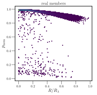
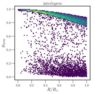
Figure 5: The distribution of the cluster membership probability $p_{\rm mem}$ as a function of the distance from the center of the cluster normalized by the richness radius $R_{\lambda}$. The left panel shows the distribution for the true members of the clusters, while the right panel shows the distribution for the interlopers. These figures imply that we cannot distinguish true members from interlopers based on the membership probabilities. Note that we use the clusters identified by using the projection length $d_{\rm cyl}^{\rm max}=60h^{-1}{\rm Mpc}$.

Next we explore the reason why the methodology does not work. As the value of $d_{\rm cyl}^{\rm max}$ is much larger than the typical radius of the halo, the optical members of the galaxy cluster invariably include a number of members which are beyond the halo, but lie along the line-of-sight to the primary halo. In Fig. 5, we show the membership probability assigned by our cluster finder as a function of the separation $R$ from the cluster center, for real members as well as interlopers. Although the membership probability does decrease as a function of radius, it can be seen that the membership probability cannot really distinguish between the interlopers and real members. Thus the method of separating the members from the interlopers using membership probability as suggested by (Zu et al., 2017), does not really solve the underlying problem.

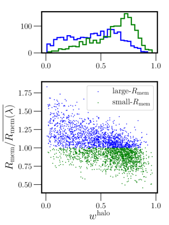
Figure 6: The figure shows the correlation between the fraction of true halo members and $R_{\rm mem}/\overline{R_{\rm mem}(\lambda)}$. The clusters split into large/small-$<R_{\rm mem}>$ subsamples are shown in blue/green dots and are divided by the horizontal line at unity. The large-$<R_{\rm mem}>$ clusters tend to contain larger fractions of interlopers than the small-$<R_{\rm mem}>$ clusters. Note that we use the cluster samples identified with the projection length of $60h^{-1}{\rm Mpc}$ here.

Due to this, the resultant value of $\langle R_{\rm mem}\rangle$ from the assigned members invariably consists of contributions from both the real members as well as the interlopers. The division by $\langle R_{\rm mem}\rangle$ automatically also results in a division based on the amount of correlated large scale structure, with large $\langle R_{\rm mem}\rangle$ corresponding to larger values of the correlated structure. This then gets reflected in the associated cross-correlation on large scales at fixed observed richness.

Mathematically, we can write down

$$\langle R_{\rm mem}\rangle=w^{\rm halo}\langle R_{\rm mem}\rangle^{\rm halo}+w^{\rm int}\langle R_{\rm mem}\rangle^{\rm int}\,,$$ (6)

where $\langle R_{\rm mem}\rangle^{\rm halo}$ and $\langle R_{\rm mem}\rangle^{\rm int}$ denote the average distance of the true members and the interlopers from the centers of optically identified cluster centers. The weights $w^{\rm halo}$ and $w^{\rm int}$ denote the weights which correspond to the fractional contribution of the members and interlopers to the total richness of the optically identified galaxy cluster system. Fig. 6 shows the distribution of the weight $w^{\rm halo}$ for the case of the projection length $d_{\rm cly}^{\rm max}=60h^{-1}{\rm Mpc}$. The small-$<R_{\rm mem}>$ clusters tend to have larger real member fraction $w^{\rm halo}$ peaked around 0.8, while the distribution of $w^{\rm halo}$ for large-$<R_{\rm mem}>$ clusters is more broadly distributed to smaller values. This implies that the large-$<R_{\rm mem}>$ clusters are more correlated with large scale structure by including more number of foreground/background galaxies.

The method adopted in Miyatake et al. (2016) and More et al. (2016) is marred by the correlation coefficient between $\langle R_{\rm mem}\rangle$ and the large scale overdensity. The interpretation of the difference in clustering amplitude for different $\langle R_{\rm mem}\rangle$ clusters seen by Miyatake et al. (2016) and More et al. (2016), thus depends upon the relative strengths of these correlations with large-scale overdensity as well as the weights $w^{\rm halo}$. The use of the shuffled galaxy catalogs completely erases out the correlation between the mean distance of true members $<R_{\rm mem}>^{\rm halo}$ and the overdensity, thus making the test entirely sensitive to just the projection effects. The fact that the shuffled and the non-shuffled catalogs give similar differences in the clustering amplitudes for the two cluster subsamples, implies that the results are dominated by projection effects, and within the error bars, it would be hard to disentangle the two.

4.2 Implications for the measurement of the splashback radius

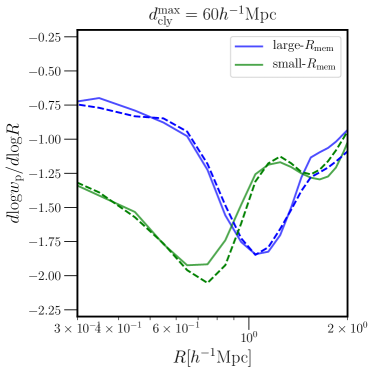
Figure 7: Logarithmic derivative profiles of the projected correlation functions of clusters in the large-$<R_{\rm mem}>$ (blue) and small-$<R_{\rm mem}>$ (green) subsamples using the projection length $d_{\rm cyl}^{\rm max}=60h^{-1}{\rm Mpc}$. The integral scale $R$ of the correlation function is $100h^{-1}{\rm Mpc}$. Solid lines are the results from the non-shuffled catalogs, while dashed lines are from the shuffled catalogs. Note that the location of the splashback radius does not depend on the choice of the integral scales. Note that these profiles are obtained by using the Savitzky-Golay algorithm to smooth the measurements. We fit a third-order polynomial over a window of five neighboring points.

Next, we measure the location of splashback radius for the optically selected galaxy clusters from our simulations. The splashback radius corresponds to the apocenter of the outermost shell in theoretical models of spherical symmetric collapse (Adhikari et al., 2014; Shi, 2016). These can be identified by locating jumps in the density distribution (Mansfield et al., 2017), or the average location of the apocenter of particles falling into the cluster potential Diemer et al. (2017). All these definitions follow the general trend of a decreasing splashback radius with increasing rate of accretion (Diemer et al., 2017). In this paper, we adopt the convention of More et al. (2015b), who define the location of the splashback radius to be the location of the steepest logarithmic slope of the radially averaged density profile, due to its ease of accessibility in data. For halos on galaxy cluster scales, which on average are accreting matter at relatively faster rates, this location corresponds to the location of the splashback radius.

We take the logarithmic derivative of the projected correlation functions and identify the location of the steepest slope as the 2-dimensional splashback radius (Diemer & Kravtsov, 2014b; More et al., 2015b). We obtain these logarithmic slopes by using the Savitzky-Golay algorithm, to smooth the projected correlation functions (More, 2016). Specifically we fit a third-order polynomial over a window of five neighboring points and then use a cubic spline to interpolate between these smoothed measurements.

The results are shown in Fig. 7 for both the non-shuffled and the shuffled cases. The solid lines are the results for large-$\langle R_{\rm mem}\rangle$ cluster subsamples, and the dashed lines for small-$\langle R_{\rm mem}\rangle$ subsamples. As is clear from the figures, the large-$\langle R_{\rm mem}\rangle$ subsamples (corresponding to low concentration subsamples) have a larger splashback radius for both non-shuffled and shuffled catalogs. We expect little difference in the results from non-shuffled and shuffled catalogs, because the distribution of galaxies within clusters (which determines the location of splashback radius) does not change much even after shuffling.

Furthermore, the location of splashback radius does not depend on either the choice of the projection length, or of the scale of integration along the line-of-sight. Therefore we decided not to show in Fig. 7. The locations of the steepest slope of the two-dimensional cross-correlations in the different $\langle R_{\rm mem}\rangle$ samples seem to be robust against these various systematics.

However, we need to investigate if projection effects in optical cluster finding can bias the measurements of the inferred location of the 3-d splashback radius significantly. After all, it is the 3-d splashback radius which contains information about the accretion rates of galaxy clusters. Typically in studies that claim the detection of the splashback radius, the projected cross-correlation between galaxy clusters and galaxies is modeled under the assumption of spherical symmetry to infer the location of the 3-d splashback radius. Given the asymmetry introduced by the projection effects along the line-of-sight due to optical cluster finding, it is important to gauge the impact of the inaccuracy of this assumption.

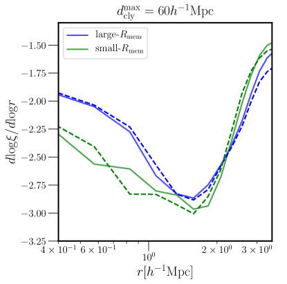
Figure 8: Logarithmic derivative profiles of the three-dimensional correlation functions $\xi_{\rm cg}(r)$ in real-space. The solid lines correspond to the derivative profiles from the non-shuffled catalogs, while the dashed lines are from the shuffled catalogs. The splashback radii are larger than the ones from the projected correlation functions and the locations are almost the same between large/small-$<R_{\rm mem}>$ subsamples.

To test this, we compute the three-dimensional cross-correlation functions $\xi_{\rm cg}(r)$ between galaxies and the large/small-$\langle R_{\rm mem}\rangle$ subsamples in real-space, as shown in Fig. 8. The splashback radii measured from the three-dimensional correlation function are larger than the one from the projected correlation function, and are almost the same unlike the case of the projected ones. The similar location of the 3d splashback radius is most probably a consequence of the similar halo mass distributions of these subsamples.

Next, we assume spherical symmetry and project $\xi_{\rm cg}(r)$ to predict the projected correlation functions using Abel transformation. If the spherical symmetry assumption holds then these predictions should match the directly measured projected correlations. The comparison in the left panel of Fig. 9, shows that these two do not agree each other. This is because spherical symmetry is broken for the clusters identified by our implementation of redMaPPer algorithm. This is more evident in the right panel of Fig.9, which compares the logarithmic derivative of these correlation functions. The difference in the location of the splashback radius between the projected correlation function and the one from $\xi_{\rm cg}(r)$ is about $15\%$. This difference is suspiciously close to the size of the difference found between the splashback radius of the redMaPPer galaxy clusters and the expectation from $\Lambda$CDM about the location of their splashback radius More et al. (2016); Baxter et al. (2017); Chang et al. (2018). Galaxy clusters selected using the Sunyaev-Zel’dovich (SZ) effect or via their X-ray emission are expected to be less severely affected by such effects, however the comparisons of the measurements of splashback radius to their expected locations are still dominated by statistical error (e.g., Umetsu & Diemer (2017); Shin et al. (2018); Zürcher & More (2019); Contigiani et al. (2019)). This also implies that the splashback radius measured from the projected correlation functions is not reliable when the clusters in the sample all have a coherent axis of asymmetry.

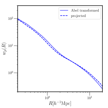
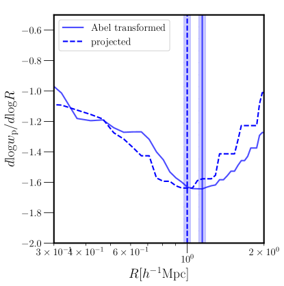
Figure 9: Left: The projected correlation functions transformed from the three-dimensional cross-correlation functions using Abel transform. Note that the three-dimensional cross-correlation functions are computed in real-space. The dashed lines are the projected cross-correlation functions. Right: Logarithmic derivative profiles of the Abel transformed correlation functions (solid) as well as the projected correlation functions (dashed). The lines correspond to the location of splashback radius, and the shaded regions show the typical errors on the measurements in real data taken from More et al. (2016). The Abel transformed correlation functions do not agree with the projected ones because spherical symmetry is broken due to projection effects.

4.3 Comparison with Observations

We now use data from the SDSS redMaPPer cluster catalog and SDSS spectroscopic galaxies and look for features similar to what we see in the simulation analysis from the previous section. To do this, we use only those redMaPPer clusters which have spectroscopic redshifts and cross-correlate them with the LOWZ spectroscopic galaxy catalogs. Unlike More et al. (2016), our use of galaxies with spectroscopic redshift allows us to map our the cross-correlation function as a function of both projected and line-of-sight separations. This allows us to evaluate the contamination due to foreground/background galaxies. In particular, we would like to test the dependence of the projected cross-correlation function on the line-of-sight integration scale as in Fig. 1 and Fig. 4.

Fig. 10 shows the ratio of the projected correlation functions between large/small-$\langle R_{\rm mem}\rangle$ cluster subsamples. Different colors correspond to different integral scales $\pi_{\rm max}$ up to $200h^{-1}{\rm Mpc}$. As is shown in the figure, the ratio keeps increasing as $\pi_{\rm max}$ increases. In the previous section, we showed that the ratio does not increase when the integral scale $\pi_{\rm max}$ becomes larger than the projection length used to find clusters. Therefore, the figure indicates that the redMaPPer clusters possibly contain some galaxies which are as far as $100h^{-1}{\rm Mpc}$ away from their centers. Due to observational limits, it is difficult to conclude that there are no foreground/background galaxies included beyond $100h^{-1}{\rm Mpc}$ even though we do not see any increase in the ratio beyond $100h^{-1}{\rm Mpc}$, because the noise becomes dominant beyond a certain scale.

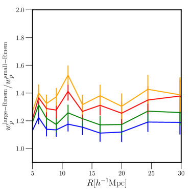
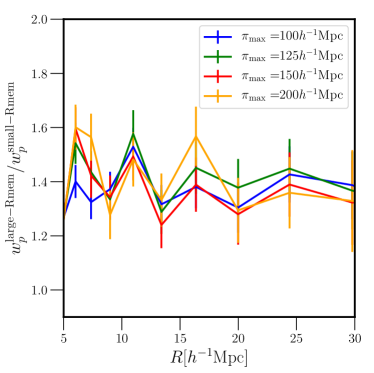
Figure 10: (Left) The ratio of the projected cross-correlation functions of large-$\langle R_{\rm mem}\rangle$ and small-$\langle R_{\rm mem}\rangle$ subsamples of the SDSS redMaPPer clusters and the LOWZ spectroscopic sample integrated up to $\pi_{\rm max}=100h^{-1}{\rm Mpc}$. Different colors correspond to different integral scale $R$. As we integrate up to $R=100h^{-1}{\rm Mpc}$, the ratio becomes larger compared to the case of $R=10h^{-1}{\rm Mpc}$ or $R=30h^{-1}{\rm Mpc}$. (Right) The same figure with the integral scale from $\pi_{\rm max}=100h^{-1}{\rm Mpc}$ to $200h^{-1}{\rm Mpc}$. After exceeding the integral scale $\pi_{\rm max}=100h^{-1}{\rm Mpc}$, we do not see the increase in the bias ratio, which implies that the possible projection effect only goes up to $100h^{-1}{\rm Mpc}$.

5 Summary

Miyatake et al. (2016) and More et al. (2016) claimed evidence for the halo assembly bias signal using the redMaPPer galaxy clusters. These studies unambiguously show that splitting the sample of the redMaPPer galaxy clusters into two subsamples based on the compactness of the member galaxies, leads to samples with similar halo masses, yet different large scale clustering amplitudes, with large scale biases of the two subsamples different by almost 60 percent. This difference was significantly larger than the expected amplitude of the assembly bias expected from numerical simulations at this mass scale.

Busch & White (2017) demonstrated that the large assembly bias signal can be reproduced in a $\Lambda$CDM framework by mimicking the optical cluster selection effects. This raised the prospect that the observational detection of assembly bias could be entirely a result of projection effects. We conducted a thorough investigation of the matter using an improved version of their implementation of the mock redMaPPer algorithm. Following is a succinct summary of our investigations and findings.

• We used a novel method in which we applied a redMaPPer like algorithm to the Millennium simulation semi-analytical galaxy catalog as well as a shuffled version of this catalog, where the signature of halo assembly bias was explicitly erased out.

• We showed that the our mock version of the redMaPPer algorithm shows features which are similar to those of the real version of redMaPPer in terms of the mass-richness relation, as well as the distribution of halo masses at fixed richness.

• We found that both the shuffled and the non-shuffled versions of the catalog, when split in to two subsamples each based on cluster-centric distances at fixed richness, show differences in clustering amplitude consistent with each other.

• Given that the shuffled catalog, has no inherent assembly bias signal, the difference in the observed clustering amplitude of the subsamples, thus, cannot be used to claim a detection of halo assembly bias signal.

• We attributed the presence of the clustering difference to the correlation induced by the optical cluster selection between the $\langle R_{\rm mem}\rangle$ of galaxy clusters, the interloper fractions, and the large scale structure overdensity modes along the line-of-sight.

• We also critically investigated the inference of the 3-d splashback radius of optically selected galaxy clusters based on the 2-d projected density profiles of galaxies around such clusters.

• We explicitly show that the asymmetry introduced by the line-of-sight projection effects in optically selected galaxy clusters hinders a straightforward inference of the 3-d splashback radius of galaxy clusters.

• We further verified that the SDSS redMaPPer clusters show the same dependence of the assembly bias signal on the line-of-sight projection length as seen in the simulations, further building circumstantial evidence for the existence of projection effects in redMaPPer optical clusters.

6 Acknowledgements

We thank useful discussions with Phillip Busch, Neal Dalal, Benedikt Diemer, Bhuvnesh Jain, Andrey Kravtsov, Yen-ting Lin, Hironao Miyatake, Ryoma Murata, Masamune Oguri, Masahiro Takada, Simon White, Ying Zu, and the organizers and participants of the KITP program: The Galaxy-Halo Connection. KITP is supported by the National Science Foundation underGrant No. NSF PHY17-48958. TS is supported by Kakenhi grant 15H05893 and 15K21733. SM is supported by Kakenhi grant 16H01089.

AppendixA: 2D correlation functions

In this paper, we discussed how projection effects differently affect the apparent assembly bias and splashback radius signals between large/small-$<R_{\rm mem}>$ subsamples. In this Appendix, we compare the two-dimensional cross correlation functions between the two subsamples. Fig. 11 shows the logarithmic ratio of 2D cross-correlation functions, ${\rm log}_{10}(b_{\rm large-R}/b_{\rm small-R})$ for various projection lengths. In the inner region, the clustering of small-$R_{\rm mem}$ subsample is stronger, and only goes to $1h^{-1}{\rm Mpc}$ in real-space while it extends to $10h^{-1}{\rm Mpc}$ in redshift-space. This trend is consistent with Busch & White (2017). On large scales, the behaviour switches and the clustering of large-$\langle R_{\rm mem}\rangle$ subsample becomes stronger.

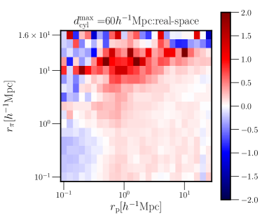
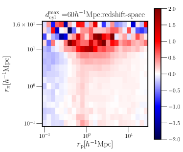
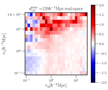
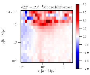
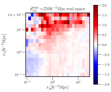
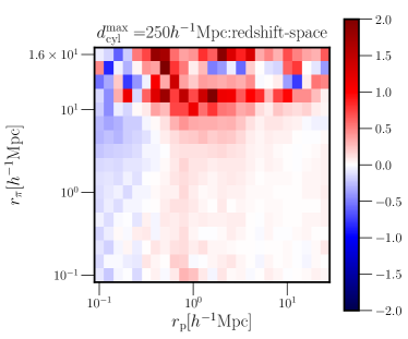
Figure 11: The logarithmic ratio of 2D cross-correlation functions between galaxies and the large/small-$<R_{\rm mem}>$ cluster subsamples, ${\rm log}_{10}(b_{\rm large-R}/b_{\rm small-R})$. The top to bottom panels correspond to different projection lengths $d_{\rm cyl}^{\rm max}=60h^{-1}{\rm Mpc}$, $120h^{-1}{\rm Mpc}$, and $250h^{-1}{\rm Mpc}$ respectively. The left column is the ratios computed in real-space, while the right column is the ratios in redshift-space. As is consistent with Busch & White (2017), the boundary is smeared out by redshift-space distortions.

References

- Adhikari et al. (2014) Adhikari S., Dalal N., Chamberlain R. T., 2014, Journal of Cosmology and Astroparticle Physics, 2014, 019
- Aihara (2011) Aihara H. e. a., 2011, ApJS, 193, 29
- Alam et al. (2015) Alam S. et al., 2015, ApJS, 219, 12
- Bartelmann (1996) Bartelmann M., 1996, A&A, 313, 697
- Baxter et al. (2017) Baxter E. et al., 2017, ApJ, 841, 18
- Busch & White (2017) Busch P., White S. D. M., 2017, MNRAS, 470, 4767
- Chang et al. (2018) Chang C. et al., 2018, ApJ, 864, 83
- Contigiani et al. (2019) Contigiani O., Hoekstra H., Bahé Y. M., 2019, MNRAS, 485, 408
- Dalal et al. (2008) Dalal N., White M., Bond J. R., Shirokov A., 2008, ApJ, 687, 12
- Diemer & Kravtsov (2014a) Diemer B., Kravtsov A. V., 2014a, ApJ, 789, 1
- Diemer & Kravtsov (2014b) Diemer B., Kravtsov A. V., 2014b, ApJ, 789, 1
- Diemer et al. (2017) Diemer B., Mansfield P., Kravtsov A. V., More S., 2017, The Astrophysical Journal, 843, 140
- Efstathiou et al. (1988) Efstathiou G., Frenk C. S., White S. D. M., Davis M., 1988, MNRAS, 235, 715
- Faltenbacher & White (2010) Faltenbacher A., White S. D. M., 2010, ApJ, 708, 469
- Gao et al. (2005) Gao L., Springel V., White S. D. M., 2005, MNRAS, 363, L66
- Gao & White (2007) Gao L., White S. D. M., 2007, MNRAS, 377, L5
- Guo et al. (2011) Guo Q. et al., 2011, MNRAS, 413, 101
- Han et al. (2018) Han J., Cole S., Frenk C. S., Benitez-Llambay A., Helly J., 2018, MNRAS, 474, 604
- Kaiser (1984) Kaiser N., 1984, ApJ, 284, L9
- Klypin et al. (2016) Klypin A., Yepes G., Gottlöber S., Prada F., Heß S., 2016, MNRAS, 457, 4340
- Lin et al. (2016) Lin Y.-T., Mandelbaum R., Huang Y.-H., Huang H.-J., Dalal N., Diemer B., Jian H.-Y., Kravtsov A., 2016, ApJ, 819, 119
- Mansfield et al. (2017) Mansfield P., Kravtsov A. V., Diemer B., 2017, The Astrophysical Journal, 841, 34
- Miyatake et al. (2016) Miyatake H., More S., Takada M., Spergel D. N., Mandelbaum R., Rykoff E. S., Rozo E., 2016, Physical Review Letters, 116, 041301
- Mo & White (1996) Mo H. J., White S. D. M., 1996, MNRAS, 282, 347
- More (2016) More S., 2016, SavGolFilterCov: Savitzky Golay filter for data with error covariance. Astrophysics Source Code Library
- More et al. (2015a) More S., Diemer B., Kravtsov A., 2015a, ArXiv e-prints
- More et al. (2015b) More S., Diemer B., Kravtsov A. V., 2015b, ApJ, 810, 36
- More et al. (2016) More S. et al., 2016, ApJ, 825, 39
- Murata et al. (2018) Murata R., Nishimichi T., Takada M., Miyatake H., Shirasaki M., More S., Takahashi R., Osato K., 2018, ApJ, 854, 120
- Navarro et al. (1997) Navarro J. F., Frenk C. S., White S. D. M., 1997, ApJ, 490, 493
- Rozo & Rykoff (2014) Rozo E., Rykoff E. S., 2014, ApJ, 783, 80
- Rozo et al. (2015a) Rozo E., Rykoff E. S., Bartlett J. G., Melin J.-B., 2015a, MNRAS, 450, 592
- Rozo et al. (2015b) Rozo E., Rykoff E. S., Becker M., Reddick R. M., Wechsler R. H., 2015b, MNRAS, 453, 38
- Rykoff et al. (2012) Rykoff E. S. et al., 2012, ApJ, 746, 178
- Rykoff et al. (2014) Rykoff E. S. et al., 2014, ApJ, 785, 104
- Shi (2016) Shi X., 2016, Monthly Notices of the Royal Astronomical Society, 459, 3711
- Shin et al. (2018) Shin T. et al., 2018, arXiv e-prints
- Springel et al. (2005) Springel V. et al., 2005, Nature, 435, 629
- Springel et al. (2001) Springel V., White S. D. M., Tormen G., Kauffmann G., 2001, MNRAS, 328, 726
- Umetsu & Diemer (2017) Umetsu K., Diemer B., 2017, ApJ, 836, 231
- van den Bosch & Ogiya (2018) van den Bosch F. C., Ogiya G., 2018, MNRAS, 475, 4066
- van den Bosch et al. (2018) van den Bosch F. C., Ogiya G., Hahn O., Burkert A., 2018, MNRAS, 474, 3043
- Wang et al. (2013) Wang L., Weinmann S. M., De Lucia G., Yang X., 2013, MNRAS, 433, 515
- Wechsler et al. (2006) Wechsler R. H., Zentner A. R., Bullock J. S., Kravtsov A. V., Allgood B., 2006, ApJ, 652, 71
- Yang et al. (2006) Yang X., Mo H. J., van den Bosch F. C., 2006, ApJ, 638, L55
- Zu et al. (2017) Zu Y., Mandelbaum R., Simet M., Rozo E., Rykoff E. S., 2017, MNRAS, 470, 551
- Zürcher & More (2019) Zürcher D., More S., 2019, ApJ, 874, 184