Non-equilibrium probability flux of a thermally driven micromachine

Abstract

We discuss the non-equilibrium statistical mechanics of a thermally driven micromachine consisting of three spheres and two harmonic springs [Y. Hosaka et al., J. Phys. Soc. Jpn. 86, 113801 (2017)]. We obtain the non-equilibrium steady state probability distribution function of such a micromachine and calculate its probability flux in the corresponding configuration space. The resulting probability flux can be expressed in terms of a frequency matrix that is used to distinguish between a non-equilibrium steady state and a thermal equilibrium state satisfying detailed balance. The frequency matrix is shown to be proportional to the temperature difference between the spheres. We obtain a linear relation between the eigenvalue of the frequency matrix and the average velocity of a thermally driven micromachine that can undergo a directed motion in a viscous fluid. This relation is consistent with the scallop theorem for a deterministic three-sphere microswimmer.

I Introduction

Microswimmers are tiny machines that swim in a fluid and they are expected to be used in microfluidics and microsystems Lauga09 . Over the length scale of microswimmers, the fluid forces acting on them are dominated by the frictional viscous forces. By transforming chemical energy into mechanical energy, however, microswimmers change their shape and move efficiently in viscous environments. According to Purcell’s scallop theorem, time-reversible body motion cannot be used for locomotion in a Newtonian fluid Purcell77 ; Lauga11 . As one of the simplest models exhibiting broken time-reversal symmetry, Najafi and Golestanian proposed a three-sphere swimmer Golestanian04 ; Golestanian08 , in which three in-line spheres are linked by two arms of varying length. Recently, such a swimmer has been experimentally realized by using colloidal beads manipulated by optical tweezers Leoni09 or by controlling ferromagnetic particles at an air-water interface Grosjean16 ; Grosjean18 .

Recently, the present authors have proposed a generalized three-sphere microswimmer model in which the spheres are connected by two harmonic springs, i.e., an elastic microswimmer Yasuda17 ; Kuroda19 . A similar model was also considered by other people Dunkel09 ; Pande15 ; Pande17 . Later, our model was further extended to a thermally driven elastic microswimmers Hosaka17 , suggesting a new mechanism for locomotion that is purely induced by thermal fluctuations without any external forcing. As depicted in Fig. 1, the key assumption is that the three spheres are in equilibrium with independent heat baths characterized by different temperatures. In such a situation, heat transfer occurs inside the micromachine from a hotter sphere to a colder one, driving the whole system out of equilibrium. We have shown that a combination of heat transfer and hydrodynamic interactions among the spheres can lead to directional locomotion in a steady state Hosaka17 . Our model has a similarity to a class of thermal ratchet models Magnasco93 ; Astumian94 ; Rousselet94 , and the suggested new mechanism is relevant to non-equilibrium dynamics of proteins and enzymes in biological systems Jee18 ; Dey19 .

For a thermally driven elastic micromachine, the average velocity was calculated to be Hosaka17

$$\langle V\rangle=\frac{k_{\rm B}(T_{3}-T_{1})}{96\pi\eta\ell^{2}},$$ (1)

where $k_{\rm B}$ is the Boltzmann constant, $T_{1}$ and $T_{3}$ are the temperatures of the first and the third spheres (see Fig. 1), $\eta$ is the viscosity of the surrounding fluid, and $\ell$ is the natural length of the two springs. This result indicates that the swimming direction is from a colder sphere to a hotter one, and the velocity does not depend on the temperature of the middle sphere. Moreover, we demonstrated that the average velocity is determined by the net heat flow between the first and the third spheres (see Sec. VI later) Hosaka17 . This result is consistent with the theoretical framework of “stochastic energetics” Sekimoto97 ; Sekimoto98 ; SekimotoBook . However, a more detailed analysis based on non-equilibrium statistical mechanics is required in order to clarify the physical mechanism for the locomotion of a thermally driven micromachine.

It is well-known that systems in thermodynamic equilibrium obey detailed balance meaning that transition rates between any two microscopic states are pairwise balanced KampenBook . For non-equilibrium steady state situations, however, detailed balance is broken and a probability flux loop should exist in a configuration phase space Weiss03 ; Weiss07 ; Ghanta17 ; Gnesotto18 . Such a probability flux has been experimentally measured in the periodic beating of a flagellum from Chlamydomonas reinhardtii and in the non-periodic fluctuations of primary cilia of epithelial cells Battle16 . A similar analysis was performed for non-equilibrium shape fluctuations of semi-flexible filaments in a viscoelastic environment Gladrow16 ; Gladrow17 . Since the existence of a probability flux loop is a direct verification of a non-equilibrium steady state, it is a useful concept to characterize driven systems.

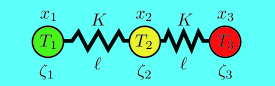
Figure 1: (Color online)　 Thermally driven elastic three-sphere micromachine. Three spheres are connected by two identical harmonic springs characterized by the elastic constant $K$ and the natural length $\ell$. The time-dependent positions of the spheres are denoted by $x_{i}(t)$ ($i=1,2,3$) in a one-dimensional coordinate system, and $\zeta_{i}$ is the friction coefficient for $i$-th sphere. The three spheres are in equilibrium with independent heat baths at temperatures $T_{i}$. In this paper, we do not take into account hydrodynamic interactions acting between different spheres.

In this paper, we discuss the non-equilibrium statistical mechanics of a thermally driven micromachine consisting of three spheres and two harmonic springs Hosaka17 . We obtain the steady state conformational distribution function of such a micromachine and calculate its probability flux in the corresponding configuration space. The obtained probability flux will be expressed in terms of a frequency matrix to discuss the non-equilibrium steady state of a micromachine. The main purpose of our work is to understand the physical mechanism that underlies the locomotion of a thermally driven micromachine within the non-equilibrium statistical mechanics. To this aim, we shall obtain a relation connecting the eigenvalue of the frequency matrix to the average velocity of a thermally driven micromachine as shown in Eq. (1). With this relation, we show explicitly that the concept of Purcell’s scallop theorem can be generalized for thermally driven micromachines. Together with the results in Ref. Hosaka17 , the present study provides an unified description of the locomotion of a stochastic elastic micromachine.

In the next Section, we explain our model of a thermally driven three-sphere micromachine by introducing the coupled Langevin equations for the two spring extensions. In Sec. III, we determine the steady state probability distribution function of an elastic micromachine. By employing the Fokker-Planck equation in Sec. IV, we obtain the steady state probability flux in the configuration space. From the Gaussian probability flux, we calculate the frequency matrix and the flux rotor. In Sec. V, the average velocity of a micromachine will be expressed in terms of the obtained quantities characterizing the scale of non-equilibrium. Finally, a summary of our work and some discussion are given in Sec. VI. In Appendix, we give a matrix representation of linear stochastic dynamical systems, which is useful to understand our results from a general point of view.

II Thermally driven three-sphere micromachine

We first explain the model of a thermally driven elastic micromachine that was introduced before by the present authors Hosaka17 . As schematically shown in Fig. 1, this model consists of three hard spheres connected by two harmonic springs. For the sake of simplicity, we assume that the two springs are identical, and the common spring constant and the natural length are given by $K$ and $\ell$, respectively. Then the total elastic energy is given by

$$E=\frac{K}{2}(x_{2}-x_{1}-\ell)^{2}+\frac{K}{2}(x_{3}-x_{2}-\ell)^{2},$$ (2)

where $x_{i}(t)$ ($i=1,2,3$) are the positions of the three spheres in a one-dimensional coordinate system, and we also assume $x_{1}<x_{2}<x_{3}$ without loss of generality. In our previous model for an elastic swimmer Yasuda17 ; Kuroda19 , the natural length of each spring was assumed to undergo a prescribed cyclic motion in time, $\ell(t)$, representing internal states of the micromachine. However, for a thermally driven micromachine Hosaka17 , as we discuss in this paper, $\ell$ is taken to be a constant.

We consider a situation in which the three spheres are in thermal equilibrium with independent heat baths at temperatures $T_{i}$ ($i=1,2,3$) Hosaka17 . When these temperatures are different, the system is inevitably driven out of equilibrium because heat flux from a hotter sphere to a colder one is generated. The equations of motion of the three spheres are written in the form of Langevin equations as

$$\dot{x}_{1} =\frac{K}{\zeta_{1}}(x_{2}-x_{1}-\ell)+\left(\frac{2T_{1}}{\zeta_{1}}\right)^{1/2}\xi_{1},$$ (3)

$$\dot{x}_{2} =-\frac{K}{\zeta_{2}}(x_{2}-x_{1}-\ell)+\frac{K}{\zeta_{2}}(x_{3}-x_{2}-\ell)$$

$$+\left(\frac{2T_{2}}{\zeta_{2}}\right)^{1/2}\xi_{2},$$ (4)

$$\dot{x}_{3} =-\frac{K}{\zeta_{3}}(x_{3}-x_{2}-\ell)+\left(\frac{2T_{3}}{\zeta_{3}}\right)^{1/2}\xi_{3},$$ (5)

where dot indicates the time derivative, $\zeta_{i}$ ($i=1,2,3$) is the friction coefficient for $i$-th sphere, and the Boltzmann constant is set to unity hereafter [except in Eqs. (51) and (53)]. Furthermore, $\xi_{i}(t)$ ($i=1,2,3$) is a zero mean and unit variance Gaussian white noise, independent for all the spheres:

$$\langle\xi_{i}(t)\rangle=0,$$ (6)

$$\langle\xi_{i}(t)\xi_{j}(t^{\prime})\rangle=\delta_{ij}\delta{(t-t^{\prime})}.$$ (7)

In contrast to Ref. Hosaka17 , we do not consider hydrodynamic interactions acting between different spheres in Eqs. (3)–(5). Hence, the locomotion of a micromachine is not explicitly taken into account in this paper, but such a treatment is sufficient for the statistical analysis of the configurational properties. Corrections due to hydrodynamic interactions will briefly be discussed in Sec. VI.

In the following argument, it is convenient to introduce the two spring extensions with respect to $\ell$:

$$r_{12}=x_{2}-x_{1}-\ell,~{}~{}~{}~{}~{}r_{23}=x_{3}-x_{2}-\ell.$$ (8)

From Eqs. (3)–(5), we obtain the Langevin equations for $r_{12}(t)$ and $r_{23}(t)$ as Grosberg15 ; Netz18

$$\dot{r}_{12} =-\frac{K}{\zeta_{12}}r_{12}+\frac{K}{\zeta_{2}}r_{23}+\left(\frac{2T_{12}}{\zeta_{12}}\right)^{1/2}\xi_{12},$$ (9)

$$\dot{r}_{23} =\frac{K}{\zeta_{2}}r_{12}-\frac{K}{\zeta_{23}}r_{23}+\left(\frac{2T_{23}}{\zeta_{23}}\right)^{1/2}\xi_{23}.$$ (10)

Here we have introduced the relevant effective friction coefficient

$$\zeta_{ij}=\frac{\zeta_{i}\zeta_{j}}{\zeta_{i}+\zeta_{j}},$$ (11)

and the mobility-weighted average temperature

$$T_{ij}=\frac{\zeta_{j}T_{i}+\zeta_{i}T_{j}}{\zeta_{i}+\zeta_{j}}.$$ (12)

The average temperatures $T_{12}$ and $T_{23}$ can be regarded as two effective temperatures characterizing non-equilibrium behaviors of a thermally driven micromachine in the reduced configuration space, i.e., in the $(r_{12},r_{23})$ space.

The definition of the effective temperature $T_{ij}$ arises from the condition that the newly defined noises $\xi_{12}(t)$ and $\xi_{23}(t)$ in Eqs. (9) and (10), respectively, satisfy the following statistical properties:

$$\langle\xi_{12}(t)\rangle=\langle\xi_{23}(t)\rangle=0,$$ (13)

$$\langle\xi_{12}(t)\xi_{12}(t^{\prime})\rangle=\delta(t-t^{\prime}),$$ (14)

$$\langle\xi_{23}(t)\xi_{23}(t^{\prime})\rangle=\delta(t-t^{\prime}),$$ (15)

$$\langle\xi_{12}(t)\xi_{23}(t^{\prime})\rangle=-\frac{T_{2}}{\zeta_{2}}\left(\frac{\zeta_{12}\zeta_{23}}{T_{12}T_{23}}\right)^{1/2}\delta(t-t^{\prime}).$$ (16)

It is important to note that the strength of the cross-correlation $\langle\xi_{12}(t)\xi_{23}(t^{\prime})\rangle$ in Eq. (16) is negative and its amplitude differs from unity. This noise property turns out to be important when we discuss the Fokker-Planck equation for the probability distribution function in Sec. IV.

III Steady state distribution function

III.1 Covariance matrix

In this Section, we shall investigate the conformational distribution of $r_{12}$ and $r_{23}$ that obey the coupled Langevin equations given by Eqs. (9) and (10). For this purpose, we introduce a Fourier representation of any function $f(t)$ as

$$f(t)=\int_{-\infty}^{\infty}\frac{d\omega}{2\pi}\,f[\omega]e^{i\omega t},$$ (17)

where $\omega$ is the frequency and $f[\omega]$ is the Fourier component. We rewrite Eqs. (9) and (10) in terms of $r_{12}[\omega]$ and $r_{23}[\omega]$ and solve for them. After some calculations, they become

$$r_{12}[\omega] =-\frac{1}{b}\biggl{[}\left(\frac{i\omega\zeta_{2}}{K}+\frac{\zeta_{2}}{\zeta_{23}}\right)\left(\frac{2T_{12}}{\zeta_{12}}\right)^{1/2}\xi_{12}[\omega]$$

$$+\left(\frac{2T_{23}}{\zeta_{23}}\right)^{1/2}\xi_{23}[\omega]\biggr{]},$$ (18)

$$r_{23}[\omega] =-\frac{1}{b}\biggl{[}\left(\frac{i\omega\zeta_{2}}{K}+\frac{\zeta_{2}}{\zeta_{12}}\right)\left(\frac{2T_{23}}{\zeta_{23}}\right)^{1/2}\xi_{23}[\omega]$$

$$+\left(\frac{2T_{12}}{\zeta_{12}}\right)^{1/2}\xi_{12}[\omega]\biggr{]},$$ (19)

where the common quantity $b$ in the denominators is

$$b=\frac{\zeta_{2}}{K}\omega^{2}-i\zeta_{2}\left(\frac{1}{\zeta_{12}}+\frac{1}{\zeta_{23}}\right)\omega+\frac{K}{\zeta_{2}}\left(1-\frac{\zeta_{2}^{2}}{\zeta_{12}\zeta_{23}}\right).$$ (20)

Using Eqs. (18) and (19), one can calculate the three correlation functions $\langle r_{12}[\omega]r_{12}[\omega^{\prime}]\rangle$, $\langle r_{23}[\omega]r_{23}[\omega^{\prime}]\rangle$, and $\langle r_{12}[\omega]r_{23}[\omega^{\prime}]\rangle$ in the frequency domain. Then the two variances $\sigma_{12}^{2}$, $\sigma_{23}^{2}$ and the covariance $\sigma_{13}$ (or the equal-time correlation functions) are obtained as

$$\sigma_{12}^{2} =\int_{-\infty}^{\infty}\frac{d\omega}{2\pi}\int_{-\infty}^{\infty}\frac{d\omega^{\prime}}{2\pi}\,\langle r_{12}[\omega]r_{12}[\omega^{\prime}]\rangle$$

$$=\frac{1}{K}(T_{12}+\zeta_{12}\Delta),$$ (21)

$$\sigma_{23}^{2} =\int_{-\infty}^{\infty}\frac{d\omega}{2\pi}\int_{-\infty}^{\infty}\frac{d\omega^{\prime}}{2\pi}\,\langle r_{23}[\omega]r_{23}[\omega^{\prime}]\rangle$$

$$=\frac{1}{K}(T_{23}+\zeta_{23}\Delta),$$ (22)

$$\sigma_{13} =\int_{-\infty}^{\infty}\frac{d\omega}{2\pi}\int_{-\infty}^{\infty}\frac{d\omega^{\prime}}{2\pi}\,\langle r_{12}[\omega]r_{23}[\omega^{\prime}]\rangle$$

$$=\frac{\zeta_{2}\Delta}{K},$$ (23)

where we have used the notation

$$\Delta=\frac{\zeta_{12}\zeta_{23}(T_{12}+T_{23}-2T_{2})}{(\zeta_{12}+\zeta_{23})(\zeta_{2}^{2}-\zeta_{12}\zeta_{23})}.$$ (24)

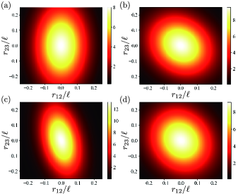
Figure 2: (Color online)　 Dimensionless probability distribution function $p({\bm{r}})\ell^{2}$ given by Eq. (30) as a function of $r_{12}/\ell$ and $r_{23}/\ell$. The parameters are (a) $\zeta_{1}=\zeta_{2}=\zeta_{3}$, $\tau_{1}=1/900$, $\tau_{2}=41/900$, and $\tau_{3}=81/900$ (these temperatures satisfy $\tau_{1}+\tau_{3}=2\tau_{2}$), (b) $\zeta_{1}=\zeta_{2}=\zeta_{3}$, $\tau_{1}=\tau_{3}=25/900$, and $\tau_{2}=41/900$, (c) $\zeta_{1}/\zeta_{2}=0.5$, $\zeta_{3}/\zeta_{2}=5$, $\tau_{1}=1/900$, $\tau_{2}=41/900$, and $\tau_{3}=81/900$ (these temperatures are the same as in (a)), (d) $\zeta_{1}/\zeta_{2}=0.5$, $\zeta_{3}/\zeta_{2}=5$, $\tau_{1}=\tau_{3}=25/900$, and $\tau_{2}=41/900$ (these temperatures are the same as in (b)).

With these results, we construct a symmetric covariance matrix $\mathbf{C}$ defined by

$${\mathbf{C}} =\begin{pmatrix}\sigma_{12}^{2}&\sigma_{13}\\ \sigma_{13}&\sigma_{23}^{2}\end{pmatrix}.$$ (25)

Then the inverse of the covariance matrix can be simply given by

$$\mathbf{C}^{-1}=\frac{1}{\sigma_{12}^{2}\sigma_{23}^{2}(1-\rho^{2})}\begin{pmatrix}\sigma_{23}^{2}&-\sigma_{13}\\ -\sigma_{13}&\sigma_{12}^{2}\end{pmatrix},$$ (26)

where the correlation factor $\rho$ is defined by

$$\rho=\frac{\sigma_{13}}{\sigma_{12}\sigma_{23}}=\frac{\zeta_{2}\Delta}{[(T_{12}+\zeta_{12}\Delta)(T_{23}+\zeta_{23}\Delta)]^{1/2}}.$$ (27)

Notice that the absolute value of the correlation factor should satisfy the condition $|\rho|<1$. As explained in Ref. Weiss03 and summarized in Appendix, the steady state covariance matrix can generally be obtained by solving the corresponding Lyapunov equation [see Eq. (59)].

When the three friction coefficients are all identical, i.e., $\zeta_{1}=\zeta_{2}=\zeta_{3}$, the above correlation factor reduces to

$$\rho=\frac{2(T_{1}+T_{3}-2T_{2})}{[(7T_{1}+4T_{2}+T_{3})(T_{1}+4T_{2}+7T_{3})]^{1/2}}.$$ (28)

Here, we see that $\rho$ generally vanishes when $T_{1}+T_{3}=2T_{2}$, i.e, the temperature of the middle sphere coincides with the average temperature between the first and the third spheres. Obviously, $\rho$ vanishes in thermal equilibrium, $T_{1}=T_{2}=T_{3}$, although $\rho=0$ does not mean that the micromachine is in thermal equilibrium.

III.2 Distribution function

Next we consider the steady state probability distribution function $p({\bm{r}})$, where ${\bm{r}}=(r_{12},r_{23})^{\mathsf{T}}$ and “${\mathsf{T}}$” indicates the transpose. Owing to the reproductive property of Gaussian distributions KampenBook , $p({\bm{r}})$ should also be a Gaussian function for the present linear problem and is given by

$$p({\bm{r}})={\cal N}\exp\left[-\frac{1}{2}{\bm{r}}^{\mathsf{T}}{\mathbf{C}}^{-1}{\bm{r}}\right],$$ (29)

where ${\cal N}$ is the normalization factor. Using Eq. (26) for ${\mathbf{C}}^{-1}$, we can write the explicit form of the distribution function as

$$p({\bm{r}})=\frac{1}{2\pi\sigma_{12}\sigma_{23}(1-\rho^{2})^{1/2}}$$

$$\times\exp\biggl{[}-\frac{1}{2(1-\rho^{2})}\biggl{(}\frac{r_{12}^{2}}{\sigma_{12}^{2}}-2\rho\frac{r_{12}r_{23}}{\sigma_{12}\sigma_{23}}+\frac{r_{23}^{2}}{\sigma_{23}^{2}}\biggr{)}\biggr{]},$$ (30)

together with Eqs. (21), (22), and (27). Despite the fact that the micromachine is out of equilibrium, the extensions of the two springs obey the Boltzmann-type distribution that is characterized by the effective temperatures $T_{12}$ and $T_{23}$ Grosberg15 . Our further analysis crucially depends on the result of Eq. (30).

Let us introduce the following dimensionless temperature parameter

$$\tau_{i}=\frac{2T_{i}}{K\ell^{2}},$$ (31)

which is the ratio between the thermal energy of each sphere and the spring elastic energy (recall $k_{\rm B}=1$). In Fig. 2, we plot the dimensionless steady state distribution function $p({\bm{r}})$ in Eq. (30) as a function of $r_{12}/\ell$ and $r_{23}/\ell$ for different parameter combinations. The absolute value of the friction coefficient is not required for these plots because we are focusing only on the stationary state distribution. The parameters in Fig. 2(a) are $\zeta_{1}=\zeta_{2}=\zeta_{3}$, $\tau_{1}=1/900$, $\tau_{2}=41/900$, and $\tau_{3}=81/900$. Notice that these temperatures satisfy $\tau_{1}+\tau_{3}=2\tau_{2}$ and hence $\rho=0$ according to Eq. (28). This means that the distribution function $p({\bm{r}})$ is simply a product of two Gaussian functions, and there is no correlation between $r_{12}$ and $r_{23}$ for these temperatures. The distribution function is elongated in the $r_{23}$-direction because $\tau_{1}<\tau_{3}$.

The parameters in Fig. 2(b) are $\zeta_{1}=\zeta_{2}=\zeta_{3}$, $\tau_{1}=\tau_{3}=25/900$, and $\tau_{2}=41/900$. Here the temperatures of the first and the third spheres are identical although the correlation factor obtained from Eq. (28) is negative, $\rho<0$. The correlation between $r_{12}$ and $r_{23}$ causes a tilt of the elongated distribution and the tilt direction has a negative slope. Here the whole plot is symmetric with respect to the straight line $r_{12}=r_{23}$. In spite of the correlation between $r_{12}$ and $r_{23}$, the system is thermally balanced because the effective temperatures $T_{12}$ and $T_{23}$ are identical. As we mention in the next Section, the micromachine behaves as if it were in thermal equilibrium in the reduced configuration space.

Keeping the temperature parameters $\tau_{i}$ the same as in Fig. 2(a) and (b), we introduce asymmetries in the friction coefficients, e.g., $\zeta_{1}/\zeta_{2}=0.5$ and $\zeta_{3}/\zeta_{2}=5$, in Fig. 2(c) and (d), respectively. Then the correlation factor should be estimated according to Eq. (27). In Fig. 2(c), there is a negative correlation between $r_{12}$ and $r_{23}$ owing to the different friction coefficients. On the other hand, Fig. 2(d) is no longer symmetric with respect to the line $r_{12}=r_{23}$. Since $T_{12}\neq T_{23}$ in this case [see Eq. (12)], the system is not thermally balanced and exhibits non-equilibrium behaviors.

So far, we have calculated the steady state conformational distribution function $p$ of a thermally driven micromachine. We have shown that it is given by a Gaussian function characterized by the covariance matrix ${\mathbf{C}}$. In the next Section, we shall calculate the probability flux by using the obtained distribution function.

IV Probability flux and related quantities

IV.1 Probability flux

Next, we calculate the probability flux that can be used to characterize the non-equilibrium properties of a three-sphere micromachine. The Fokker-Planck equation corresponding to Eqs. (9) and (10) can be written for the time-dependent conformational probability distribution function $p({\bm{r}},t)$ as RiskenBook ; ZwanzigBook

$$\dot{p}=-\nabla\cdot{\bm{j}},$$ (32)

expressing the fact that probability is neither created nor annihilated. In the above, the two-dimensional nabla operator indicates $\nabla=(\partial/\partial r_{12},\partial/\partial r_{23})^{\mathsf{T}}$ in the configuration space and the vector ${\bm{j}}=(j_{12},j_{23})^{\mathsf{T}}$ is the two-dimensional probability flux given by

$${\bm{j}}={\mathbf{A}}{\bm{r}}p-{\mathbf{D}}\nabla p,$$ (33)

where the matrices ${\mathbf{A}}$ and ${\mathbf{D}}$ are

$${\mathbf{A}}=\begin{pmatrix}-K/\zeta_{12}&K/\zeta_{2}\\ K/\zeta_{2}&-K/\zeta_{23}\end{pmatrix},$$ (34)

and

$${\mathbf{D}}=\begin{pmatrix}T_{12}/\zeta_{12}&-T_{2}/\zeta_{2}\\ -T_{2}/\zeta_{2}&T_{23}/\zeta_{23}\end{pmatrix},$$ (35)

respectively. Here ${\mathbf{A}}$ describes the linear deterministic dynamics (without noise) in Eqs. (9) and (10), whereas ${\mathbf{D}}$ is called the diffusion matrix (see also Appendix). The non-zero off-diagonal components of ${\mathbf{D}}$ originate from the noise correlation shown in Eq. (16).

In a steady state, i.e., $\dot{p}=0$, the probability flux ${\bm{j}}({\bm{r}})$ can be obtained from Eq. (33) by using the Gaussian probability distribution function $p$ in Eq. (30):

$$j_{12}({\bm{r}}) =\biggl{[}K\biggl{(}\frac{r_{23}}{\zeta_{2}}-\frac{r_{12}}{\zeta_{12}}\biggr{)}+\frac{1}{(1-\rho^{2})}\biggl{\{}\frac{T_{12}r_{12}}{\zeta_{12}\sigma_{12}^{2}}$$

$$+\frac{\rho}{\sigma_{12}\sigma_{23}}\biggl{(}\frac{T_{2}r_{12}}{\zeta_{2}}-\frac{T_{12}r_{23}}{\zeta_{12}}\biggr{)}-\frac{T_{2}r_{23}}{\zeta_{2}\sigma_{23}^{2}}\biggr{\}}\biggr{]}p,$$ (36)

$$j_{23}({\bm{r}}) =\biggl{[}K\biggl{(}\frac{r_{12}}{\zeta_{2}}-\frac{r_{23}}{\zeta_{23}}\biggr{)}+\frac{1}{(1-\rho^{2})}\biggl{\{}-\frac{T_{2}r_{12}}{\zeta_{2}\sigma_{12}^{2}}$$

$$+\frac{\rho}{\sigma_{12}\sigma_{23}}\biggl{(}\frac{T_{2}r_{23}}{\zeta_{2}}-\frac{T_{23}r_{12}}{\zeta_{23}}\biggr{)}+\frac{T_{23}r_{23}}{\zeta_{23}\sigma_{23}^{2}}\biggr{\}}\biggr{]}p.$$ (37)

One can confirm that this probability flux is divergence-free, i.e., $\nabla\cdot{\bm{j}}=0$, so that the steady state condition is satisfied.

IV.2 Frequency matrix

The above probability flux ${\bm{j}}$ can be conveniently expressed in terms of a frequency matrix ${\bm{\Omega}}$ as Weiss03

$${\bm{j}}={\bm{\Omega}}{\bm{r}}p,$$ (38)

where the explicit expression of ${\bm{\Omega}}$ is given by

$${\bm{\Omega}}=\begin{pmatrix}\displaystyle-\frac{K}{\zeta_{12}}+\frac{1}{(1-\rho^{2})}\left(\frac{T_{12}}{\zeta_{12}{\sigma_{12}}^{2}}+\frac{\rho T_{2}}{\sigma_{12}\sigma_{23}\zeta_{2}}\right)&\displaystyle\frac{K}{\zeta_{2}}-\frac{1}{(1-\rho^{2})}\left(\frac{T_{2}}{\zeta_{2}{\sigma_{23}}^{2}}+\frac{\rho T_{12}}{\sigma_{12}\sigma_{23}\zeta_{12}}\right)\\[8.61108pt] \displaystyle\frac{K}{\zeta_{2}}-\frac{1}{(1-\rho^{2})}\left(\frac{T_{2}}{\zeta_{2}{\sigma_{12}}^{2}}+\frac{\rho T_{23}}{\sigma_{12}\sigma_{23}\zeta_{23}}\right)&\displaystyle-\frac{K}{\zeta_{23}}+\frac{1}{(1-\rho^{2})}\left(\frac{T_{23}}{\zeta_{23}{\sigma_{23}}^{2}}+\frac{\rho T_{2}}{\sigma_{12}\sigma_{23}\zeta_{2}}\right)\end{pmatrix}.$$ (39)

Since ${\bm{j}}$ is divergence-free, ${\bm{\Omega}}$ should be a traceless matrix Weiss07 . Using Eqs. (11) and (12), we indeed find that ${\bm{\Omega}}$ is traceless. In Appendix, we generally show that the frequency matrix ${\bm{\Omega}}$ can be expressed as ${\bm{\Omega}}={\mathbf{A}}+{\mathbf{D}}{\mathbf{C}}^{-1}$ within the matrix formulation [see Eq. (61)].

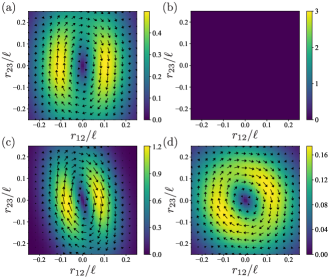
Figure 3: (Color online)　 Dimensionless probability flux vector ${\bm{j}}({\bm{r}})\zeta_{2}\ell/K$ given by Eq. (38) as a function of $r_{12}/\ell$ and $r_{23}/\ell$. The parameter values are the same as in Fig. (2). There is no probability flux in (b). The color scale indicates the magnitude of the flux vector ${\bm{j}}$.

When the friction coefficients are identical, $\zeta_{1}=\zeta_{2}=\zeta_{3}=\zeta$, the frequency matrix is simplified to

$${\bm{\Omega}} =\frac{K(T_{1}-T_{3})}{\zeta c}$$

$$\times\begin{pmatrix}2(T_{1}+T_{3}-2T_{2})&-(7T_{1}+4T_{2}+T_{3})\\ T_{1}+4T_{2}+7T_{3}&-2(T_{1}+T_{3}-2T_{2})\end{pmatrix},$$ (40)

where the quantity $c$ in the denominators is

$$c=T_{1}^{2}+16T_{1}T_{2}+14T_{1}T_{3}+16T_{2}T_{3}+T_{3}^{2}.$$ (41)

Here, we explicitly see that ${\bm{\Omega}}$ is proportional to $T_{1}-T_{3}$, and hence the probability flux ${\bm{j}}$ vanishes when $T_{1}=T_{3}$ for any $T_{2}$ of the middle sphere. Indeed, ${\bm{j}}=0$ or ${\bm{\Omega}}=0$ is a necessary and sufficient condition for physical situations in which detailed balance is satisfied Weiss03 . When the system is in thermal equilibrium and detailed balance holds, the probability of a transition between any two states is the same as the probability of the reverse transition. As a result, a net probability flux does not exist. In Appendix, we generally show that the necessary and sufficient condition for detailed balance is given by the commutation relation ${\mathbf{A}}{\mathbf{D}}-{\mathbf{D}}{\mathbf{A}}^{\mathsf{T}}=0$ [see Eq. (62)].

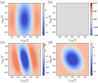
Figure 4: (Color online)　 Dimensionless flux rotor $s({\bm{r}})\zeta_{2}\ell^{2}/K$ given by Eq. (43) as a function of $r_{12}/\ell$ and $r_{23}/\ell$. The parameter values are the same as in Fig. (2). There is no flux rotor in (b).

When $T_{1}\neq T_{3}$, on the other hand, we have non-zero frequency matrix ${\bm{\Omega}}$. Then detailed balance is violated and the micromachine is in a non-equilibrium steady state. Hence the frequency matrix is an important measure to quantify the out of equilibrium properties of a thermally driven micromachine. When $T_{1}\neq T_{3}$, the two eigenvalues of ${\bm{\Omega}}$ in Eq. (40) are given by

$$\gamma=\pm\frac{i\sqrt{3}K(T_{1}-T_{3})}{\zeta c^{1/2}}.$$ (42)

Since these eigenvalues are purely imaginary, the probability current in the configuration space is rotational Weiss03 ; Gnesotto18 . In the above, the essential frequency scale is set by $\gamma\sim K/\zeta$ which characterizes the speed of the rotational motion.

In Fig. 3, we plot the dimensionless probability flux vector ${\bm{j}}({\bm{r}})$ in Eq. (38) as a function of $r_{12}/\ell$ and $r_{23}/\ell$ by using the same parameter values as in Fig. 2. Note that the color scale indicates the magnitude of the flux vector. In Fig. 3(a), (c), and (d), clockwise flux loops can be clearly seen. When the friction coefficients are identical as in Fig. 3(a), the existence of a flux loop is consistent with a directed motion of a three-sphere micromachine Hosaka17 , as we further discuss in Sec. V.

In Fig. 3(b) with $\tau_{1}=\tau_{3}$, however, the probability flux does not exist simply because ${\bm{\Omega}}=0$. Asymmetries both in the temperatures and the friction coefficients lead to a flux loop in Fig. 3(c). The presence of a flux loop in Fig. 3(d) even for $\tau_{1}=\tau_{3}$ is due to the asymmetry in the friction coefficients. Although the case with different friction coefficients was not studied in Ref. Hosaka17 , we expect that a finite flux loop leads to a directed motion of a three-sphere micromachine despite the balanced temperature distribution.

IV.3 Flux rotor

To further characterize the strength of the probability flux loop in terms of a scalar quantity, we consider the following flux rotor Dotsenko13 :

$$s({\bm{r}}) =\frac{\partial}{\partial r_{12}}j_{23}-\frac{\partial}{\partial r_{23}}j_{12}$$

$$=\frac{p(w_{0}+w_{12}r_{12}^{2}+w_{23}r_{23}^{2}+w_{13}r_{12}r_{23})}{\zeta_{2}\zeta_{12}\zeta_{23}\sigma_{12}^{4}\sigma_{23}^{4}(1-\rho^{2})^{2}},$$ (43)

where $w_{0}$, $w_{12}$, $w_{23}$, and $w_{13}$ are

$$w_{0} =\sigma_{12}^{2}\sigma_{23}^{2}(1-\rho^{2})[\zeta_{12}\zeta_{23}T_{2}(\sigma_{12}^{2}-\sigma_{23}^{2})$$

$$+\zeta_{2}\sigma_{12}\sigma_{23}\rho(\zeta_{23}T_{12}-\zeta_{12}T_{23})],$$ (44)

$$w_{12} =[\zeta_{2}\sigma_{12}\sigma_{23}\rho(\zeta_{12}T_{23}-\zeta_{23}T_{12})$$

$$-K\zeta_{23}\sigma_{12}^{2}\sigma_{23}(1-\rho^{2})(\zeta_{12}\sigma_{23}-\zeta_{2}\sigma_{12}\rho)$$

$$+\zeta_{12}\zeta_{23}T_{2}(\sigma_{23}^{2}-\rho^{2}\sigma_{12}^{2})]\sigma_{23}^{2},$$ (45)

$$w_{23} =[\zeta_{2}\sigma_{12}\sigma_{23}\rho(\zeta_{12}T_{23}-\zeta_{23}T_{12})$$

$$-K\zeta_{12}\sigma_{12}\sigma_{23}^{2}(1-\rho^{2})(\zeta_{2}\sigma_{23}\rho-\zeta_{23}\sigma_{12})$$

$$-\zeta_{12}\zeta_{23}T_{2}(\sigma_{12}^{2}-\rho^{2}\sigma_{23}^{2})]\sigma_{12}^{2},$$ (46)

$$w_{13} =[2\zeta_{12}\zeta_{23}T_{2}\rho(\sigma_{12}^{2}-\sigma_{23}^{2})$$

$$+K\zeta_{2}\sigma_{12}\sigma_{23}(1-\rho^{2})(\zeta_{12}\sigma_{23}^{2}-\zeta_{23}\sigma_{12}^{2})$$

$$+\zeta_{2}\sigma_{12}\sigma_{23}(1+\rho^{2})(\zeta_{23}T_{12}-\zeta_{12}T_{23})]\sigma_{12}\sigma_{23}.$$ (47)

In Fig. 4, we plot the dimensionless flux rotor $s({\bm{r}})$ in Eq. (43) as a function of $r_{12}/\ell$ and $r_{23}/\ell$ by using the same parameter values as in Fig. 2. In Fig. 4(a), (c), and (d), the flux rotor $s$ takes negative values around the origin of the configuration space, ${\bm{r}}=0$, whereas it takes positive values in the outer regions. In Fig. 4(a), the distribution of $s$ is elongated in the $r_{23}$-direction, while there is no correlation between $r_{12}$ and $r_{23}$. The flux rotor vanishes in Fig. 4(b) simply because ${\bm{\Omega}}=0$ for $\tau_{1}=\tau_{3}$. When the friction coefficients are different as in Fig. 4(c) and (d), the flux rotor exhibits a negative correlation.

As considered in Ref. Dotsenko13 , one can focus on the strength of the flux rotor at the origin of the configuration space, i.e, $s({\bm{r}}=0)$. This quantity, denoted as $s_{0}$, is given by

$$s_{0}=\frac{1}{2\pi\zeta_{2}\zeta_{12}\zeta_{23}\sigma_{12}^{3}\sigma_{23}^{3}(1-\rho^{2})^{3/2}}$$

$$\times\left[\zeta_{12}\zeta_{23}T_{2}(\sigma_{12}^{2}-\sigma_{23}^{2})+\zeta_{2}\sigma_{12}\sigma_{23}\rho(\zeta_{23}T_{12}-\zeta_{12}T_{23})\right],$$ (48)

because only the term proportional to $w_{0}$ in Eq. (43) remains. When the friction coefficients are identical, $\zeta_{1}=\zeta_{2}=\zeta_{3}=\zeta$, Eq. (48) further reduces to

$$s_{0}=\frac{16\sqrt{3}K^{2}(T_{1}+T_{2}+T_{3})(T_{1}-T_{3})}{\pi\zeta c^{3/2}},$$ (49)

where $c$ is given by Eq. (41). Here the sign of $s_{0}$ is purely determined by the temperature difference $T_{1}-T_{3}$. In Fig. 5, we plot the dimensionless $s_{0}$ as a function of $T_{1}/T_{2}$ and $T_{3}/T_{2}$ by using a color representation.

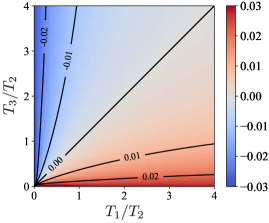
Figure 5: (Color online)　 Dimensionless flux rotor $\pi\zeta T_{2}s_{0}/(16\sqrt{3}K^{2})$ given by Eq. (49) as a function of $T_{1}/T_{2}$ and $T_{3}/T_{2}$. The flux rotor is evaluated at ${\bm{r}}=0$ when the friction coefficients are identical. Different curves are the contour lines for the corresponding values.

In this Section, starting from the Fokker-Planck equation, we have obtained the steady state probability flux ${\bm{j}}$ that can be expressed in terms of the frequency matrix ${\bm{\Omega}}$. The eigenvalues $\gamma$ of the frequency matrix are purely imaginary and proportional to the temperature difference. We have also calculated the flux rotor $s$ as a scalar quantity to characterize the scale of non-equilibrium of a micromachine. In the next Section, we shall discuss the relation between these quantities and the average velocity of a stochastic micromachine.

V Average velocity of a micromachine

As mentioned before, the main purpose of this paper is to understand the physical mechanism that underlies the locomotion of a thermally driven micromachine within the non-equilibrium statistical mechanics. When the friction coefficients are identical, the average velocity is given by Eq. (1) which is proportional to $T_{1}-T_{3}$. This proportionality appears in several scalar quantities such as the eigenvalues of the frequency matrix, $\gamma$ [see Eq. (42)], or the flux rotor at the origin, $s_{0}$ [see Eq. (49)]. Hence one can construct linear relations between the average velocity and these scalar quantities.

For example, the absolute value of the average velocity can be expressed in terms of $\gamma$ as

$$|\langle V\rangle|=\frac{a}{16\sqrt{3}\ell^{2}}\frac{c^{1/2}}{K}|\gamma^{\prime\prime}|,$$ (50)

where we have used Stokes’ law, $\zeta=6\pi\eta a$, for the friction coefficient of a hard sphere, and $\gamma^{\prime\prime}$ indicates the imaginary part of $\gamma$. For the sake of completeness, we rewrite the above expression by recovering the Boltzmann constant and using Eq. (41) as follows:

$$|\langle V\rangle|=\frac{a}{16\sqrt{3}\ell^{2}}$$

$$\times\frac{k_{\rm B}(T_{1}^{2}+16T_{1}T_{2}+14T_{1}T_{3}+16T_{2}T_{3}+T_{3}^{2})^{1/2}}{K}|\gamma^{\prime\prime}|.$$ (51)

As mentioned before, $\gamma^{\prime\prime}$ has the dimension of frequency and it determines the speed of the rotational motion of the probability flux in the configuration space.

An interesting interpretation of the above expression can be made by comparing it to the general form for the average velocity of a three-sphere swimmer. When the two arms undergo a prescribed deterministic motion, as in the original Najafi-Golestanian model Golestanian04 , the average velocity is given by Golestanian08

$$\overline{V}=\frac{G}{2}\overline{(r_{12}\dot{r}_{23}-\dot{r}_{12}r_{23})},$$ (52)

where $G\sim a/\ell^{2}$ is a geometric factor that depends only on the structural parameters of a swimmer, and the averaging is performed by time integration in a full cycle. In the above form, the averaging part is proportional to the enclosed area (per unit time) that is swept in a full cycle in the configuration space. Equation (52) can be regarded as a mathematical representation of Purcell’s scallop theorem for a three-sphere swimmer in low-Reynolds-number fluids Purcell77 ; Lauga11 .

For a thermally driven micromachine, $\langle V\rangle$ is proportional to $a/\ell^{2}$ as in Eq. (52). Moreover, $c^{1/2}$ in Eq. (50) can be regarded as overall thermal energy, and $c^{1/2}/K$ essentially represents the explored area in the configuration space by random motions of the spheres. This interpretation is reasonable because one can easily confirm the relation $c^{1/2}/K\sim\sigma_{12}\sigma_{23}$, where $\sigma_{12}$ and $\sigma_{23}$ are the variances in Eqs. (21) and (22), respectively.

While the time scale in the Najafi-Golestanian model is given by the frequency of the periodic arm motions Golestanian08 , the corresponding time scale for a thermally driven micromachine is set by the eigenvalue $\gamma$ of the frequency matrix [see Eq. (42)]. Hence Eq. (50) or Eq. (51) provides us with an essential understanding concerning the locomotion of a thermally driven micromachine. It is interesting to note that the main concept of Purcell’s scallop theorem can be generalized for thermally driven micromachines that undergo random motions rather than deterministic cyclic motions.

In order to take into account the sign of the average velocity, namely, the direction of the locomotion, it is convenient to use the flux rotor at the origin $s_{0}$ [see Eq. (49)]. After recovering the Boltzmann constant, the average velocity can also be written as

$$\langle V\rangle=-\frac{\pi a}{256\sqrt{3}\ell^{2}}$$

$$\times\frac{k_{\rm B}^{2}(T_{1}^{2}+16T_{1}T_{2}+14T_{1}T_{3}+16T_{2}T_{3}+T_{3}^{2})^{3/2}}{K^{2}(T_{1}+T_{2}+T_{3})}s_{0}.$$ (53)

In the above, the sign of $s_{0}$ determines the direction of the locomotion. For example, when $T_{1}<T_{3}$ as in Fig. 4(a) or in Fig. 5, we have $s_{0}<0$ and $\langle V\rangle>0$. Although Eqs. (51) and (53) are essentially equivalent, we consider that Eq. (51) gives more physical insights to understand the locomotion of a thermally driven micromachine.

VI Summary and discussion

In this paper, we have discussed the non-equilibrium statistical mechanics of a thermally driven micromachine made of three spheres and two harmonic springs as previously proposed by the present authors Hosaka17 . First, we have calculated the steady state conformational distribution function of such a micromachine and showed that it is given by a Gaussian function characterized by the covariance matrix [see Eq. (30)]. Using this distribution function, we have obtained the steady state probability flux of a micromachine.

The distribution function can be expressed in terms of a traceless frequency matrix [see Eqs. (39) and (40)]. When the friction coefficients are all identical, we have shown that the eigenvalues of the frequency matrix are proportional to the temperature difference between the first and the third spheres [see Eq. (40)]. Moreover, the scale of non-equilibrium of a micromachine can quantitatively be characterized by the flux rotor [see Eq. (43) or Eq. (48)]. As one of the main results of this paper, the average velocity of a thermally driven machine is expressed in terms of the eigenvalue of the frequency matrix [see Eq. (50)]. This expression allows us to generalize the concept of Purcell’s scallop theorem that is also applicable for thermally driven stochastic micromachines.

An interesting situation to be discussed in more detail is the case when $\zeta_{1}=\zeta_{2}=\zeta_{3}$ and $T_{1}=T_{3}\neq T_{2}$. Microscopically, such a micromachine is in a non-equilibrium steady state because the temperature of the second sphere is different from those of the other two spheres. However, within the configuration space $(r_{12},r_{23})$, the two relevant average temperatures are equal, i.e., $T_{12}=T_{23}$. Hence the overall state of a micromachine is effectively in thermal equilibrium and detailed balance is satisfied, i.e., ${\bm{\Omega}}=0$. This is the reason why the average velocity in Eq. (1) vanishes when $T_{1}=T_{3}$ regardless of the value of $T_{2}$.

It is known that for some non-equilibrium systems, broken detailed balance doest not need to be apparent at larger scales, and they can regain thermodynamic equilibrium when the system is coarse grained Egolf00 ; Rupprecht16 . In our analysis, the reduction of the configuration space has been implicitly assumed because we have focused only on the distribution of $r_{12}$ and $r_{23}$, while the center of mass motion of a micromachine has been neglected. Within this level of description, an elastic three-sphere micromachine behaves as if it were in thermal equilibrium when $T_{1}=T_{3}$.

In our previous paper Hosaka17 , we argued that the average velocity of a micromachine can be related to the ensemble average of heat flows in a steady state. According to “stochastic energetics”, the heat gained by $i$-th sphere per unit time is expressed as Sekimoto97 ; Sekimoto98 ; SekimotoBook

$$\dot{Q}_{i}=\zeta_{i}(-\dot{x}_{i}+\xi_{i})\dot{x}_{i},$$ (54)

where $\dot{x}_{i}(t)$ and $\xi_{i}(t)$ are given in Eqs. (3)–(5). When the friction coefficients are identical, we showed that the average velocity can also be expressed in terms of the lowest-order average heat flows as

$$\langle V\rangle=\frac{a}{8K\ell^{2}}(\langle\dot{Q}_{3}\rangle-\langle\dot{Q}_{1}\rangle).$$ (55)

This relation states that the average velocity is determined by the net heat flow between the first and the third spheres. Our result in this paper indicates that the net heat flow between the first and the third spheres is also proportional to the eigenvalue of the frequency matrix $\gamma$ or the flux rotor $s_{0}$, as discussed in Sec. V.

We mention here that our model of a three-sphere micromachine has a similarity to that of two over-damped, tethered spheres coupled by a harmonic spring and also confined between two walls Gnesotto18 ; Battle16 . Because these two spheres are in contact with heat baths having different temperatures, the system can be driven out of equilibrium. They numerically showed that displacements obey a Gaussian distribution and also found probability flux loops that demonstrate the broken detailed balance Battle16 . In Ref. Gnesotto18 , an analytical expression of the frequency matrix for this two-sphere model was shown to be proportional to the temperature difference.

Clearly, the two displacements $r_{12}$ and $r_{23}$ in Eq. (8) correspond to the sphere positions in their model. It is interesting to note, for example, that our result of the frequency matrix in Eq. (40) reduces to Eq. (42) in Ref. Gnesotto18 when $T_{2}=0$. When $T_{2}\neq 0$, however, the presence of the middle sphere changes the structure of the frequency matrix as we have shown in Eq. (39) or Eq. (40). Moreover, the important outcome of this work is the relation between the average velocity and the eigenvalue of the frequency matrix for a three-sphere micromachine [see Eq. (50) or Eq. (51)]. Notice that a two-sphere micromachine in a viscous fluid cannot have a directed motion even if the temperatures are different Hosaka17 .

As mentioned before, we have neglected long-ranged hydrodynamic interactions acting between different spheres. In our previous paper Hosaka17 , we explicitly took into account hydrodynamic interactions when the friction coefficients are all identical. If hydrodynamic interactions are taken into account in the present analysis, the variances and the covariance in Eqs. (21)–(23) are modified in non-equilibrium situations. Such hydrodynamic corrections should be proportional to $a/\ell$ within the lowest-order expansion. Moreover, such corrections should vanish in thermal equilibrium, i.e., $T_{1}=T_{2}=T_{3}$ because hydrodynamic interactions should not affect equilibrium statistical properties.

In the presence of hydrodynamic interactions, a thermally driven elastic micromachine can undergo a directional motion Hosaka17 . The presence of the middle sphere is essential for a directional motion because the hydrodynamic interactions among the three spheres are responsible for it. Such a locomotion should be distinguished from the traditional thermophoresis (Ludwig-Soret effect) in which a temperature gradient in an external fluid induces a directed motion of suspended particles Jiang10 . In our model, the locomotion of a micromachine is purely induced by non-equilibrium fluctuations of internal degrees of freedom. Here, the three spheres are in thermal equilibrium with independent heat baths having different temperatures, which is different from a situation where a temperature gradient is externally imposed in a surrounding fluid Jiang10 . For example, we showed before both analytically and numerically that a two-sphere elastic micromachine cannot move even if the temperatures are different Hosaka17 . This clearly indicates that the locomotion of a thermally driven micromachine cannot be explained within the standard thermophoresis, although it is closely related to Purcell’s scallop theorem for microswimmers under the force-free condition.

In the present work, we have shown that asymmetries in the friction coefficients lead to a finite probability flux loop [see Fig. 3(d)] or flux rotor [see Fig. 4(d)], anticipating a locomotion of an asymmetric micromachine in a viscous fluid. This prediction will be investigated in the future by performing numerical simulations of the coupled stochastic equations, as given by Eqs. (3)–(5), in the presence of hydrodynamic interactions. Notice that analytical treatment of a case with different sphere sizes is more difficult because one needs to take into account higher-order contributions in $r_{12}$ and $r_{23}$ as well as in the sphere size $a$.

So far, various concepts have been proposed to quantitatively discuss whether a steady state is in thermal equilibrium or not Rupprecht16 . One of the most promising methods is to search for the violation of the fluctuation-dissipation relation that is guaranteed in thermal equilibrium situations Guo14 ; Turlier16 . However, it is not always easy to perform two separate measures of the correlation function and of the response function for the same system. Moreover, the measurement of the response function can often be intrinsically invasive and is not suitable for biological systems. Moreover, the observation of non-Gaussian distribution fluctuations is not a proof for the non-equilibrium steady sate Bustamante05 ; Battle16 . Since the emergence of probability flux loops is a direct verification of a non-equilibrium steady state, it can be a powerful method to study systems that are driven out of equilibrium. We consider that a thermally driven three-sphere micromachine is an excellent example to show the usefulness of such an analysis.

Appendix A Matrix representation of stochastic dynamical systems

Following closely the argument in Refs. Weiss03 ; Weiss07 , we shall briefly review the general formulation of stochastic dynamical systems using a matrix representation. Let us start from the following linear stochastic Langevin model

$$\dot{{\bm{r}}}={\mathbf{A}}{\bm{r}}+{\bm{\xi}},$$ (56)

where ${\bm{r}}$ is a $N$-dimensional vector characterizing the state of the system, ${\mathbf{A}}$ is a $N\times N$-dimensional matrix describing the linear deterministic dynamics, and ${\bm{\xi}}$ is a $N$-dimensional vector representing the noise forcing. The time-dependent covariance matrix is introduced by ${\mathbf{C}}=\langle{\bm{r}}(t){\bm{r}}^{\mathsf{T}}(t^{\prime})\rangle$. Then the diffusion matrix ${\mathbf{D}}$ is defined by the relation

$$\langle{\bm{\xi}}(t){\bm{\xi}}^{\mathsf{T}}(t^{\prime})\rangle=2{\mathbf{D}}\delta(t-t^{\prime}).$$ (57)

From Eq. (56), one can show that the time evolution of the covariance matrix is given by

$$\dot{{\mathbf{C}}}={\mathbf{A}}{\mathbf{C}}+{\mathbf{C}}{\mathbf{A}}^{\mathsf{T}}+2{\mathbf{D}}.$$ (58)

When the system is in a steady state, i.e., $\dot{{\mathbf{C}}}=0$, the covariance matrix must obey the following Lyapunov equation:

$${\mathbf{A}}{\mathbf{C}}+{\mathbf{C}}{\mathbf{A}}^{\mathsf{T}}+2{\mathbf{D}}=0.$$ (59)

Hereafter, we use the same notation ${\mathbf{C}}$ for the covariance matrix that satisfies the Lyapunov equation. It should be emphasized that the Lyapunov equation holds both in equilibrium and out of equilibrium situations. Hence it can be regarded as a generalized fluctuation-dissipation relation connecting the fluctuations ($\mathbf{C}$) and the deterministic dissipation ($\mathbf{A}$).

For linear systems with Gaussian noise, the steady state probability distribution function $p$ is a Gaussian function as in Eq. (29). In this case, the probability flux defined by Eq. (33) becomes

$${\bm{j}}={\mathbf{A}}{\bm{r}}p-{\mathbf{D}}\nabla p=({\mathbf{A}}+{\mathbf{D}}{\mathbf{C}}^{-1}){\bm{r}}p,$$ (60)

Hence the frequency matrix ${\bm{\Omega}}$ introduced through the relation ${\bm{j}}={\bm{\Omega}}{\bm{r}}p$ [see Eq. (38)] is given by

$${\bm{\Omega}}={\mathbf{A}}+{\mathbf{D}}{\mathbf{C}}^{-1}.$$ (61)

When ${\bm{\Omega}}=0$ and hence detailed balance holds, we have ${\mathbf{A}}+{\mathbf{D}}{\mathbf{C}}^{-1}=0$. After the elimination of ${\mathbf{C}}$ in the Lyapunov equation, we then have

$${\mathbf{A}}{\mathbf{D}}-{\mathbf{D}}{\mathbf{A}}^{\mathsf{T}}=0.$$ (62)

This commutation relation holds if and only if the system is in thermal equilibrium and satisfies detailed balance. Moreover, whether or not detailed balance is satisfied is coordinate invariant Weiss03 .

When ${\bm{\Omega}}\neq 0$ and hence detailed balance is broken, the system is in non-equilibrium steady state situations. In this case, one can show that the following two relations hold:

$${\mathbf{A}}{\mathbf{C}}+{\mathbf{D}}={\bm{\Omega}}{\mathbf{C}},~{}~{}~{}~{}~{}{\mathbf{C}}{\mathbf{A}}^{\mathsf{T}}+{\mathbf{D}}=-{\bm{\Omega}}{\mathbf{C}}.$$ (63)

Obviously, the sum of these two relations gives again the Lyapunov equation in Eq. (59). One can also show that the flow field, as expressed by ${\bm{\Omega}}{\bm{r}}$, is perpendicular to the gradient of the probability distribution, i.e., $({\bm{\Omega}}{\bm{r}})\cdot\nabla p=0$ Gnesotto18 .

Last but not least, the matrices ${\mathbf{C}}$ in Eq. (25), ${\mathbf{A}}$ in Eq. (34), ${\mathbf{D}}$ in Eq. (35), and ${\bm{\Omega}}$ in Eq. (39) obtained for a three-sphere micromachine satisfy all the relations in this Appendix.

References

- (1) E. Lauga and T. R. Powers, Rep. Prog. Phys. 72, 096601 (2009).
- (2) E. M. Purcell, Proc. Natl. Acad. Sci. U.S.A. 94, 11307 (1997).
- (3) E. Lauga, Soft Matter 7, 3060 (2011).
- (4) A. Najafi and R. Golestanian, Phys. Rev. E 69, 062901 (2004).
- (5) R. Golestanian and A. Ajdari, Phys. Rev. E 77, 036308 (2008).
- (6) M. Leoni, J. Kotar, B. Bassetti, P. Cicuta, and M. C. Lagomarsino, Soft Matter 5, 472 (2009).
- (7) G. Grosjean, M. Hubert, G. Lagubeau, and N. Vandewalle, Phys. Rev. E 94, 021101(R) (2016).
- (8) G. Grosjean, M. Hubert, and N. Vandewalle, Adv. Colloid Interface Sci. 255, 84 (2018).
- (9) K. Yasuda, Y. Hosaka, M. Kuroda, R. Okamoto, and S. Komura, J. Phys. Soc. Jpn. 86, 093801 (2017).
- (10) M. Kuroda, K. Yasuda, and S. Komura, J. Phys. Soc. Jpn. 88, 054804 (2019).
- (11) J. Dunkel and I. M. Zaid, Phys. Rev. E 80, 021903 (2009).
- (12) J. Pande and A.-S. Smith, Soft Matter 11, 2364 (2015).
- (13) J. Pande, L. Merchant, T. Krüger, J. Harting, and A.-S. Smith, New J. Phys. 19, 053024 (2017).
- (14) Y. Hosaka, K. Yasuda, I. Sou, R. Okamoto, and S. Komura, J. Phys. Soc. Jpn. 86, 113801 (2017).
- (15) M. O. Magnasco, Phys. Rev. Lett. 71, 1477 (1993).
- (16) R. D. Astumian and M. Bier, Phys. Rev. Lett. 72, 1766 (1994).
- (17) J. Rousselet, L. Salome, A. Ajdari, and J. Prost, Nature 370, 446 (1994).
- (18) A.-Y. Jee, S. Dutta, Y.-K. Cho, T. Tlusty, and S. Granick, Proc. Natl. Acad. Sci. U.S.A. 115, 14 (2018).
- (19) K. K. Dey, Angew. Chem. Int. Ed. 58, 2208 (2019).
- (20) K. Sekimoto, J. Phys. Soc. Jpn. 66, 1234 (1997).
- (21) K. Sekimoto, Prog. Theor. Phys. Suppl. 130, 17 (1998).
- (22) K. Sekimoto, Stochastic Energetics (Springer, Berlin Heidelberg, 2010).
- (23) N. van Kampen, Stochastic Processes in Physics and Chemistry (North-Holland, Amsterdam, 1992).
- (24) J. B. Weiss, Tellus A 55, 208 (2003).
- (25) J. B. Weiss, Phys. Rev. E 76, 061128 (2007).
- (26) A. Ghanta, J. C. Neu, and S. Teitsworth, Phys. Rev. E 95, 032128 (2017).
- (27) F. S. Gnesotto, F. Mura, J. Gladrow, and C. P. Broedersz, Rep. Prog. Phys. 81, 066601 (2018).
- (28) C. Battle, C. P. Broedersz, N. Fakhri, V. F. Geyer, J. Howard, C. F. Schmidt, and F. C. MacKintosh, Science 352, 604 (2016).
- (29) J. Gladrow, N. Fakhri, F. C. MacKintosh, C. F. Schmidt, and C. P. Broedersz, Phys. Rev. Lett. 116, 248301 (2016).
- (30) J. Gladrow, C. P. Broedersz, and C. F. Schmidt, Phys. Rev. E 96, 022408 (2017).
- (31) A. Y. Grosberg and J.-F. Joanny, Phys. Rev. E 92, 032118 (2015).
- (32) R. R. Netz, J. Chem. Phys. 148, 185101 (2018).
- (33) H. Risken, The Fokker-Planck equation: Methods of solution and applications (Springer-Verlag, Berlin, 1984).
- (34) R. Zwanzig, Nonequilibrium Statistical Mechanics (Oxford University Press, New York, 2001).
- (35) V. Dotsenko, A. Maciołek, O. Vasilyev, and G. Oshanin, Phys. Rev. E 87, 062130 (2013).
- (36) D. A. Egolf, Science 287, 101 (2000).
- (37) J.-F. Rupprecht and J. Prost, Science 352, 514 (2016).
- (38) H.-R. Jiang, N. Yoshinaga, and M. Sano, Phys. Rev. Lett. 105, 268302 (2010).
- (39) M. Guo, A. J. Ehrlicher, M. H. Jensen, M. Renz, J. R. Moore, R. D. Goldman, J. Lippincott-Schwartz, F. C. MacKintosh, and D. A. Weitz, Cell 158, 822 (2014).
- (40) H. Turlier, D. A. Fedosov, B. Audoly, T. Auth, N. S. Gov, C. Sykes, J.-F. Joanny, G. Gompper, and T. Betz, Nature Physics 12, 513 (2016).
- (41) C. Bustamante, J. Liphardt, and F. Ritort, Phys. Today 58, 43 (2005).