Dark sector evolution in Horndeski models

Abstract

We use the Equation of State (EoS) approach to study the evolution of the dark sector in Horndeski models, the most general scalar-tensor theories with second order equations of motion. By including the effects of the dark sector into our code EoS_class, we demonstrate the numerical stability of the formalism and excellent agreement with results from other publicly available codes for a range of parameters describing the evolution of the function characterising the perturbations for Horndeski models, $\alpha_{\rm x}$, with ${\rm x}=\{{\rm K},{\rm B},{\rm M},{\rm T}\}$. After demonstrating that on sub-horizon scales ($k\gtrsim 10^{-3}\leavevmode\nobreak\ {\rm Mpc}^{-1}$ at $z=0$) velocity perturbations in both the matter and the dark sector are typically subdominant with respect to density perturbations in the equation of state for perturbations, we find an attractor solution for the dark sector gauge-invariant density perturbation $\Delta_{\rm ds}$ by neglecting its time derivatives in the equation describing its time evolution, as commonly done in the well-known quasi-static approximation. Using this result, we provide simplified expressions for the equation-of-state functions: the dark sector entropy perturbations $w_{\rm ds}\Gamma_{\rm ds}$ and anisotropic stress $w_{\rm ds}\Pi_{\rm ds}$. From this we derive a growth factor-like equation for both matter and dark sector and are able to capture the relevant physics for several observables with great accuracy. We finally present new analytical expressions for the well-known modified gravity phenomenological functions $\mu$, $\eta$ and $\Sigma$ for a generic Horndeski model as functions of $\alpha_{\rm x}$. We show that on small scales they reproduce expressions presented in previous works, but on large scales, we find differences with respect to other works.

1 Introduction

There is a solid amount of observational data suggesting that our Universe is currently undergoing accelerated expansion. All current data, ranging from the Cosmic Microwave Background (CMB) radiation [1, 2, 3], Type Ia supernovae [4, 5, 6] and Large Scale Structure (LSS) [7, 8, 9, 10] can be well described within the standard cosmological model, known as $\Lambda$CDM, where the cosmological constant $\Lambda$ is responsible for the accelerated expansion and the cold dark matter (CDM) component determines the evolution of cosmic structures. While the former contributes to about 68% of the present cosmic energy budget and the latter to about 28%, the remaining 4% is ordinary baryonic matter with small but non-negligible contributions from radiation and relativistic species, e.g. neutrinos [1]. In this context, the cosmological constant is generally interpreted as the energy of the vacuum and gravitational laws are those of General Relativity, assumed to be valid on all scales.

Despite the very good agreement between theoretical predictions and observational results, the cosmological constant is far from being a satisfactory explanation, especially when interpreted in the context of quantum field theory [11]. This has opened the door to an intensive theoretical effort to explore different explanations for the accelerated expansion and to investigate dark energy and modified gravity models [12, 13, 14, 15, 16, 17, 18], in particular scalar-tensor theories.

The most general scalar-tensor model with second order equations of motion is described by the Horndeski Lagrangian [19, 20, 21]. Most dark energy and modified gravity models (quintessence [22, 23, 24], $k$-essence [25, 26], KGB [27, 28, 29, 30], $f(R)$ [31, 32, 33], Brans-Dicke [34], Galileon cosmology [35, 36, 37], Gauss-Bonnet models [38]) are subclasses of the Horndeski Lagrangian. In this work we study the Horndeski Lagrangian and analyse specific subclasses.

Understanding the evolution of cosmological perturbations and their effects on observables such as the CMB and the matter power spectrum is important to fully characterise cosmological models. To do so, one relies on Einstein-Boltzmann codes which solve the linearised Einstein and Boltzmann equations on an expanding background. These codes have usually been designed to study perturbations in a standard $\Lambda$CDM model, for instance CMBFAST [39], DASh [40], CMBEASY [41], CAMB [42] and CLASS [43, 44].

Recently, the CAMB and CLASS codes have been extended to include models beyond the $\Lambda$CDM paradigm with EFTCAMB [45, 46], hi_class [47] and our previous code CLASS_EOS_FR [48], respectively, for example. Two independent implementations, COOP [49], and a recent extension of hi_class [50], allow to even study models beyond Horndeski. All these codes are based on the Effective Field Theory (EFT) formalism in its different flavours [51, 52, 53, 54] and their predictions were recently shown to agree at the sub-percent level [55]. EFCLASS [56, 57] implements an effective fluid approach for $f(R)$ models in the subhorizon approximation and for designing Horndeski. Here we extend our previous code and implement the full Horndeski dynamics into CLASS, using the Equation of State (EoS) approach [58, 59, 60, 61, 62, 63].

The EoS approach is a powerful formalism based on the identification of all modifications to General Relativity with an effective fluid described by a non-trivial stress-energy tensor $U_{\mu\nu}$. At background order this is completely specified by the choice of an equation of state $P_{\rm ds}=w_{\rm ds}\rho_{\rm ds}$, where ${\rm ds}$ denotes the dark sector (the scalar field and its effective fluid representation), while at linear perturbation order two new (perturbed) gauge-invariant equations of state are introduced, the entropy perturbations $w_{\rm ds}\Gamma_{\rm ds}$ and the anisotropic stress $w_{\rm ds}\Pi_{\rm ds}$. In this approach one studies the evolution of the density ($\Delta_{\rm ds}$) and velocity ($\Theta_{\rm ds}$) perturbations of the dark fluid and by knowing these quantities it is possible, as we will show later, to describe and compute the phenomenology of the model under consideration in a relatively simple way.

The paper is organised as follows. In Sect. 2 we briefly discuss the background and perturbation dynamics of the Horndeski models and introduce the particular subclasses analysed in this work. In Sect. 3 we review the theoretical foundations of the EoS formalism and describe our numerical implementation into our code EoS_class. In Sect. 4 we validate our code with results from hi_class, similarly to what was done in [55]. In Sect. 5 we present our numerical results on the evolution of the dark sector and of the phenomenological functions parameterizing modified gravity models. Using the fundamental equations of the EoS formalism and following the discussion in [48], we prove the existence of an attractor solution whose validity is established by comparing it with the numerical results of the code, under the assumption that velocity perturbations in the EoS are subdominant with respect to density perturbations. These considerations allow us to reproduce and extend analytical results available in the literature and provide expressions describing the phenomenology of modified gravity models. In Sect. 6 we study the phenomenology of modified gravity models. We conclude in Sect. 7.

In Appendix A we present the background expressions of the full Horndeski models, while in Appendix B we show the expressions for the four functions $\alpha_{\rm x}$, ${\rm x}=\{{\rm K},{\rm B},{\rm M},{\rm T}\}$, modelling linear perturbations according to the EFT formalism. In Appendix C we present the full expression of the EoS coefficients. Finally, in Appendix D we report the precision parameters used for the numerical comparisons, similar to those in Appendix C of [55].

In the following we use natural units with $c=\hbar=1$ and a metric with positive signature. We choose the same fiducial cosmology as in the hi_class paper [47]: the CMB temperature $T_{\rm CMB}=2.725{\rm K}$, the dimensionless Hubble parameter $h=0.675$, flat spatial geometry $\Omega_{\rm k}=0$, baryon density parameter today $\omega_{\rm b}=\Omega_{\rm b}h^{2}=0.022$, cold dark matter density parameter today $\omega_{\rm CDM}=\Omega_{\rm CDM}h^{2}=0.12$, effective number of neutrino species $N_{\rm eff}=3.046$, dark sector density parameter today, as inferred by the closure relation ($\sum_{i}\Omega_{i}=1$), $\Omega_{\rm ds}=0.688$. For all the models, the normalisation of the amplitude of perturbations is $A_{\rm s}=2.215\times 10^{-9}$, the slope of the primordial power spectrum is $n_{\rm s}=0.962$ and the reionization redshift is $z_{\rm reio}=11.36$. The background equation of state for the dark sector is $w_{\rm ds}=-1$ and it is kept fixed in the numerical analysis.

2 Horndeski gravity models

2.1 Background

Horndeski models [19, 20, 21] represent the most general Lagrangian for scalar-tensor theories leading to second order equations of motion in space and time. Their Lagrangian is given by the sum of the four following Lagrangians which encode the dynamics of the scalar field in the Jordan frame with metric $g_{\mu\nu}$ [54]:

$${\cal L}_{2} \equiv G_{2}(\phi,X)\,,$$ (2.1)

$${\cal L}_{3} \equiv G_{3}(\phi,X)\Box\phi\,,$$ (2.2)

$${\cal L}_{4} \equiv G_{4}(\phi,X)R-2G_{4,X}(\phi,X)\left[\left(\Box\phi\right)^{2}-\left(\nabla_{\mu}\nabla_{\nu}\phi\right)^{2}\right]\,,$$ (2.3)

$${\cal L}_{5} \equiv G_{5}(\phi,X)G_{\mu\nu}\nabla^{\mu\nu}\phi+\frac{1}{3}G_{5,X}(\phi,X)\left[\left(\Box\phi\right)^{3}-3\Box\phi\left(\nabla_{\mu}\nabla_{\nu}\phi\right)^{2}+2\left(\nabla_{\mu}\nabla_{\nu}\phi\right)^{3}\right]\,,$$ (2.4)

where $\phi$ and $X=g^{\mu\nu}\nabla_{\mu}\phi\nabla_{\nu}\phi$ are the scalar field and its canonical kinetic term, respectively, $R$ is the Ricci scalar and $G_{\mu\nu}$ the Einstein tensor. The subscript $X$ denotes the derivative with respect to the canonical kinetic term $X$, i.e. $G_{i,X}\equiv\partial G_{i}/\partial X$. We also have the following short-hand for compactness: $\left(\nabla_{\mu}\nabla_{\nu}\phi\right)^{2}=\left(\nabla_{\mu}\nabla_{\nu}\phi\right)\left(\nabla^{\mu}\nabla^{\nu}\phi\right)$ and $\left(\nabla_{\mu}\nabla_{\nu}\phi\right)^{3}=\left(\nabla_{\mu}\nabla_{\nu}\phi\right)\left(\nabla^{\sigma}\nabla^{\nu}\phi\right)\left(\nabla_{\sigma}\nabla^{\mu}\phi\right)$.

The functions $G_{i}$ are arbitrary functions of both $\phi$ and $X$ and it is thanks to this freedom that Horndeski models enjoy a rich phenomenology. General Relativity plus the cosmological constant is recovered when $G_{2}=-M_{\rm pl}^{2}\Lambda$, $G_{4}=M_{\rm pl}^{2}/2$ and $G_{3}=G_{5}=0$, with $M_{\rm pl}=1/\sqrt{8\pi G}$ the reduced Planck mass. Other models, such as quintessence [64], $k$-essence [25, 65], kinetic gravity braiding (KGB) [27, 28], Brans-Dicke [34], covariant Galileons [36, 37], $f(R)$ [66] and $f(G)$ [38] can be recovered by a suitable choice of the free functions, see for example Table 1 of [53].

Let us now consider the total action of the system, including the matter sector described by the action $S_{\rm m}$,

$$S=\int\mathrm{d}^{4}x\,\sqrt{-g}\,{\cal L}+S_{\rm m}\,,$$ (2.5)

where $g$ is the determinant of the metric and the scalar field Lagrangian ${\cal L}$ is ${\cal L}=\sum_{i=2}^{5}{\cal L}_{i}$, where the functions ${\cal L}_{i}$ are defined in Eqs. (2.1)–(2.4). By matter sector, we mean all the species other than the scalar field, i.e. CDM, baryons, photons and neutrinos. By dark sector we mean the scalar field and its effective fluid representation.

By varying Eqn. (2.5) with respect to the metric and the scalar field, we obtain the field equations and the equation of motion of the scalar field, respectively. In a compact way, the gravitational- and scalar-field equations read

$$-2M_{\rm pl}^{2}\sum_{i=2}^{5}{\cal G}_{\mu\nu}^{i}=-T_{\mu\nu}^{\rm m}\,,\quad\sum_{i=2}^{5}\left(\nabla^{\mu}J_{\mu}^{i}-P_{\phi}^{i}\right)=0\,,$$ (2.6)

respectively, where $i=1$ is not written because it corresponds to a simple cosmological constant and is included in the $i=2$ term in this formalism. In the previous expression, $T_{\mu\nu}^{\rm m}$ represents the stress-energy tensor for the matter components. Since the precise expressions for ${\cal G}_{\mu\nu}^{i}$, $J_{\mu}^{i}$ and $P_{\phi}^{i}$ are rather cumbersome, we do not report them here, but we refer the reader to [21, 67].

In full generality, the stress-energy tensor for the Horndeski Lagrangian describes an imperfect fluid, whose components are its energy density $\rho$, pressure $P$, energy flow $q_{\mu}$ and anisotropic stress $\pi_{\mu\nu}$.

Assuming a flat FLRW metric at the background level, $\mathrm{d}s^{2}=-\mathrm{d}t^{2}+a^{2}(t)\mathrm{d}\mathbf{x}^{2}$, the expressions above simplify considerably. Taking into account that the velocity component for the scalar field is defined as $u_{\mu}=(\nabla_{\mu}\phi)/\dot{\phi}=\delta_{\mu}^{0}$ to satisfy the metric symmetries, it is easy to find the corresponding expressions for the density $\rho_{\rm ds}$ and the pressure $P_{\rm ds}$ of the dark sector fluid associated to the scalar field [68, 69, 70]. We report the full expressions in Appendix A, Eqs. (A.1) and (A.2), respectively. Then the background quantities satisfy the standard continuity equation:

$$\dot{\rho}_{\rm ds}+3H(\rho_{\rm ds}+P_{\rm ds})=0\,.$$ (2.7)

The equation of motion for the scalar field is now [68, 69]

$$\frac{1}{a^{3}}\frac{\mathrm{d}}{\mathrm{d}t}(a^{3}J)=P_{\phi}\,,$$ (2.8)

where the expressions for $J$ [Eqn. (A.3)] and $P_{\phi}$ [Eqn. (A.4)] are given in Appendix A. Due to the Bianchi identities, Eqn. (2.8) is equivalent to the continuity equation (2.7).

2.2 Effective Field Theory parametrisation of Horndeski models

To study the evolution of the perturbations in dark energy and modified gravity models, several methods have been proposed. Among them, we recall the Effective Field Theory (EFT) approach [53, 52, 51, 54] which will be useful to describe linear perturbations in Horndeski models.

The EFT approach identifies a few functions, only depending on time, which are consistent with the background symmetries and which act as multiplying factors to the operators encoding the scale dependence of the system, see e.g. Eqn. (86) in [54]. Since the equations of motion are at most second order, in the Fourier space we expect terms of order $k^{2}$, where $k$ is the wavenumber of a mode. For Horndeski models, it turns out that four time-dependent functions are sufficient to describe the entirety of modifications to perturbations, while the background evolution is fully described by the equation of state $P_{\rm ds}=w_{\rm ds}\rho_{\rm ds}$. These four functions only depend on background quantities, such as the scalar field $\phi$, the Hubble parameter $H$, and their respective derivatives. Hence, once the Lagrangian is specified, it is easy to explicitly write down the four time-dependent functions, as well as the Hubble parameter, in terms of the $G_{i}$ functions in Eqs. (2.1)–(2.4). Here we follow [53] and use four functions {$\alpha_{\rm K}$, $\alpha_{\rm B}$, $\alpha_{\rm M}$, $\alpha_{\rm T}$}. The expressions linking the $\alpha_{\rm x}$ functions, with ${\rm x}=\{{\rm K},{\rm B},{\rm M},{\rm T}\}$, to the $G_{i}$ functions are shown in Appendix B. Let us now recall the main properties associated with the $\alpha_{\rm x}$ functions.

The kineticity, $\alpha_{\rm K}$, affects only scalar perturbations and receives contributions from all of the $G_{i}$ functions. It is the only term describing perfect fluid (no energy flow and anisotropic stress) dark energy models. When $\alpha_{\rm K}$ increases, the sound speed in the dark sector fluid decreases and eventually leads to a sound horizon smaller than the cosmological horizon. As a consequence, there is dark energy clustering on scales larger than the sound horizon. For constraints on $\alpha_{\rm K}$, see [71, 72, 73].

The braiding, $\alpha_{\rm B}$, also only affects scalar perturbations and receives contributions from the functions $G_{3}$, $G_{4}$ and $G_{5}$ in Eqs. (2.2)–(2.4). The braiding refers to the mixing of the kinetic terms of the scalar field and of the metric as can be appreciated in Eqn. (86) of [54]. It modifies the coupling between matter and curvature, giving rise to an additional fifth force which is usually described as a modification of the effective Newton’s constant in the equations of motion of the perturbations [48].

The rate of running of the Planck mass, $\alpha_{\rm M}$, affects both the scalar and the tensor perturbations and gets contributions from $G_{4}$ and $G_{5}$ only. A value different from zero leads to anisotropic stress, ultimately yielding differences between the gravitational potentials $\phi$ and $\psi$.

Finally, the tensor speed excess, $\alpha_{\rm T}$, represents the deviations of the speed of gravitational waves $c_{\rm T}$ from that of light: $c_{\rm T}^{2}=1+\alpha_{\rm T}$. It receives contributions from $G_{4}$ and $G_{5}$ and leads to anisotropic stress. This quantity was extensively discussed after the detection of the gravitational wave signal GW170817, due to binary neutron star merger. Indeed, the almost simultaneous detection of GW170817 and its electromagnetic counterpart excludes models with $\alpha_{\rm T}\neq 0$ to high significance [74, 75, 76], presuming that the Horndeski model applies on all scales. This implies $G_{5}=0$ and $G_{4}=G_{4}(\phi)$. See [77, 78, 70] for a review of Horndeski models surviving constraints from GW170817 and [79, 80, 81] for earlier works on the implications of a luminal propagation for GW. We note that some models can evade these constraints provided they have a scale-dependent tensor speed excess, or are Lorentz-violating or are non-local [82].

A generic model might suffer from instabilities leading to exponentially unstable perturbations. Horndeski models can be unstable for several reasons, for example when specifying the $\alpha_{\rm x}$s arbitrarily without linking them to the actual scalar theory or when a given background equation of state $w_{\rm ds}$ leads to the wrong sign of the kinetic term. This is, for example, the case for $f(R)$ models, where, despite allowing a background with $w_{\rm ds}<-1$, the corresponding perturbation sector is unstable, as discussed in [48], where it was shown that a vast sector of $f(R)$ theories with $w_{\rm ds}\neq-1$ can be ruled out by current cosmological data.

Perturbations can face three specific varieties of instabilities: ghost instabilities arise when the kinetic term is negative; gradient instabilities arise when the sound speed squared is negative, affecting small scale modes most strongly; tachyon instabilities arise when the mass squared is negative.

In Horndeski models, the stability of perturbations requires the following quantities to be positive [83, 53, 54]:

• $\alpha\equiv\alpha_{\rm K}+6\alpha_{\rm B}^{2}$, which represents the kinetic coefficient and hence the absence of ghosts;

• the sound speed squared of scalar perturbations, $c_{\rm s}^{2}$;

• the sound speed squared of tensor perturbations, $c_{\rm T}^{2}$;

• $M^{2}$, which represents the effective Planck mass squared.

These stability conditions are implemented in our code EoS_class as is the case in the hi_class code.

2.3 Specific classes of models used as examples in our analysis

In our numerical implementation, we assume an exact $\Lambda$CDM background expansion and specific phenomenological parametrisation of the $\alpha_{\rm x}$ functions, with ${\rm x}=\{{\rm K},{\rm B},{\rm M},{\rm T}\}$. In particular, following the previous literature, we chose $\alpha_{\rm x}(a)=\alpha_{\rm x,0}\,\Omega_{\rm ds}(a)$, where $\Omega_{\rm ds}(a)$ is the dark energy density parameter and $\alpha_{\rm x,0}$ an arbitrary fixed number. We also introduce the effective Planck mass $M^{2}$, via

$$\alpha_{\rm M}\equiv\frac{\mathrm{d}\ln{M^{2}}}{\mathrm{d}\ln{a}}\,.$$

For $M^{2}$ to be uniquely determined, one needs to specify initial conditions. Here we choose $M^{2}/M_{\rm pl}^{2}=1$ at early times, i.e. $a\ll 1$. Following [47], we will also fix $\alpha_{\rm K,0}=1$ for the kineticity term, as it has been shown that this function is very difficult to constrain with data, as observables are weakly dependent on $\alpha_{\rm K}$.

In contrast to [47], we do not consider models with $\alpha_{\rm B}=\alpha_{\rm M}=0$ and $\alpha_{\rm T}\neq 0$. Indeed, it is impossible to construct a Lagrangian with $\alpha_{\rm M}\equiv 0$ and $\alpha_{\rm T}\neq 0$ because to achieve the first condition, excluding extreme fine-tuning between $G_{4}$ and $G_{5}$, one requires $M^{2}$ constant, and therefore $G_{4}$ and $G_{5}$ must be constant, which forces $\alpha_{\rm T}=0$, contradicting the original assumption. Further it is also impossible to have $a_{\rm B}=0$ and $a_{\rm T}\neq 0$ because, unless there is a fine-tuning (different from the previous one) between $G_{3}$, $G_{4}$ and $G_{5}$, $a_{\rm B}\equiv 0$ also implies $G_{4}$ and $G_{5}$ constant and hence $a_{\rm T}=0$, again in disagreement with the original assumption. We note that, always under the assumption of $a_{\rm B}=0$, $G_{3}\equiv G_{3}(\phi)$, which due to an integration by parts, is equivalent to a $k$-essence model with $G_{2}\rightarrow G_{2}-G_{3,\phi}\nabla_{\mu}\phi\nabla^{\mu}\phi$.

Therefore, we consider the following classes of models:

1. $k$-essence-like models: $\alpha_{\rm K}\neq 0$, $\alpha_{\rm B}=\alpha_{\rm M}=\alpha_{\rm T}=0$. This choice corresponds to Quintessence [22, 23, 24] and $k$-essence models [25, 26] and in terms of the Horndeski Lagrangian requires $G_{2}=G_{2}(\phi,X)$, $G_{4}=M_{\rm pl}^{2}/2$ and $G_{3}=G_{5}=0$. Expressions for the EoS for perturbations can be found in [59, 62]. The numerical implementation of this class of models has been studied many times before and we will not discuss these models further.

2. $f(R)$-like models: $\alpha_{\rm K}=\alpha_{\rm T}=0$, $\alpha_{\rm M}\neq 0$, $\alpha_{\rm B}\neq 0$. From the definition of the $\alpha_{\rm x}$s coefficients in Appendix B in terms of the Horndeski functions $G_{i}$, again excluding fine-tuning between the Horndeski functions, one requires $G_{2}=G_{2}(\phi)$, $G_{4}=G_{4}(\phi)$ and $G_{3}=G_{5}=0$. This is indeed the case for $f(R)$ gravity models [31, 32, 33], which represent a particular subclass of these models where $\alpha_{\rm M}=2\alpha_{\rm B}$ as $G_{2}=-\tfrac{1}{2}M_{\rm pl}^{2}(Rf_{R}-f)$ and $G_{4}=\tfrac{1}{2}M_{\rm pl}^{2}(1+f_{R})$, where $f_{R}=\mathrm{d}f/\mathrm{d}R$. Indeed, one can show [see for example, 33, 85] that $f(R)$ models are equivalent to Brans-Dicke models [34] with the parameter $\omega_{\rm BD}=0$ and with the identification $\phi/M_{\rm pl}=1+f_{R}$ and scalar field potential $V(\phi)=-G_{2}$, where $R\equiv R(\phi)$. In this paper we do not show numerical results for $f(R)$ gravity, as this was the subject of our previous works [63, 48, 55]. The EoS for $f(R)$ gravity can be found in [63, 48]. We note that unlike hi_class, our code is able to solve the equations of motion in this class of models.

3. KGB-like models: $\alpha_{\rm K}\neq 0$, $\alpha_{\rm B}\neq 0$, $\alpha_{\rm M}=\alpha_{\rm T}=0$. These models have $G_{2}=G_{2}(\phi,X)$, $G_{3}=G_{3}(\phi,X)$, $G_{4}=M_{\rm pl}^{2}/2$ and $G_{5}=0$ and describe KGB-like gravity [27, 28, 29, 30]. The expressions for the EoS parameters have been evaluated by [60] and we verified that the expressions used here are equivalent to those found there. As we will show later, it is possible to write the EoS in terms of the matter and dark sector fluid variables, while [60] used metric variables. To establish the equivalence of the two expressions, it is useful to consider the gauge-invariant quantities $X$, $Y$ (introduced in Sect. 5.1) defined as linear combinations of the metric perturbations and their time derivatives. By writing the entropy as perturbations in both the Newtonian and synchronous gauge in terms of the gauge invariant quantities, it is relatively easy to find what conditions the coefficients must obey in order to ensure gauge invariance. This then leads to the equality of the expressions given here with those presented in [60].

4. $\alpha_{\rm K}\neq 0$, $\alpha_{\rm M}\neq 0$, $\alpha_{\rm B}=\alpha_{\rm T}=0$. A luminal propagation of GW, $\alpha_{\rm T}=0$, requires $G_{5}=0$ and $G_{4}=G_{4}(\phi)$, while $\alpha_{\rm B}=0$ implies $XG_{3,X}+G_{4,\phi}=0$. We are then free to write $G_{4}(\phi)=\tfrac{1}{2}M_{\rm pl}^{2}f(\phi/M_{\rm pl})$, with $f(\phi/M_{\rm pl})$ a dimensionless function of the scalar field $\phi$, leads to $G_{3}=-\tfrac{1}{2}M_{\rm pl}\left[f^{\prime}\left(\phi/M_{\rm pl}\right)\ln{\left(X/m^{4}\right)}+g\left(\phi/M_{\rm pl}\right)\right]$, where the prime stands for the derivative with respect to $\phi/M_{\rm pl}$, $m$ is an arbitrary mass scale and $g(\phi/M_{\rm pl})$ a dimensionless function of $\phi$. These models also have $G_{2}=G_{2}(\phi,X)$.

5. $\alpha_{\rm K}\neq 0$, $\alpha_{\rm B}\neq 0$, $\alpha_{\rm M}\neq 0$, $\alpha_{\rm T}=0$. This represents the most generic Horndeski model compatible with GW constraints. It is obtained by setting $G_{2}=G_{2}(\phi,X)$, $G_{3}=G_{3}(\phi,X)$, $G_{4}=G_{4}(\phi)$ and $G_{5}=0$. In addition to models already mentioned under classes 1–4, models falling in this category are non-minimally coupled $k$-essence [86, 87], MSG/Palatini $f(R)$ models [88, 89], Galileon cosmology [35]. Note that often for these classes of models, there exists a relation between $\alpha_{\rm B}$ and $\alpha_{\rm M}$. This is for example the case of the no slip gravity model proposed by [90] which has $\alpha_{\rm B}=\alpha_{\rm M}$ and of the minimally self-accelerating models of [79, 81] designed to break the dark degeneracy. Model 4 is a subclass of model 5, provided that $G_{3}$ is suitably chosen to give $\alpha_{\rm B}=0$.

6. $\alpha_{\rm K}\neq 0$, $\alpha_{\rm B}\neq 0$, $\alpha_{\rm M}\neq 0$, $\alpha_{\rm T}\neq 0$. This is the most general Horndeski model allowed by the theory. The free functions are all depending on $\phi$ and $X$. Typical classes of models are given by Galileons [36, 37] and Gauss-Bonnet models [38]. These models are in tension with gravitational waves measurements, but we include them for completeness.

3 The Equation of State approach and its numerical implementation

We have implemented the EoS approach for the scalar sector in a way similar to the implementation presented in our most recent analyses [48, 91] with some minor differences. For clarity let us recall the main equations and definitions of our new implementation.

We use the density perturbation $\Delta$ and the rescaled velocity perturbation $\Theta$, defined as

$$\Delta\equiv\delta+\Theta\,,\quad\Theta\equiv 3H(1+w)\theta\,.$$ (3.1)

In Eqn. (3.1), $H$ is the Hubble parameter, $w=\bar{P}/\bar{\rho}$ the background equation of state, $\delta=\delta\rho/\bar{\rho}$ the density perturbation and $\theta$ the divergence of the velocity perturbation. Overbarred variables refer to background quantities.

We introduce the gauge invariant rescaled velocity perturbation

$$\hat{\Theta}\equiv\Theta+3(1+w)T\,,$$ (3.2)

where $T=0$ in the conformal Newtonian gauge (CNG) and $T=(h^{\prime}+6\eta^{\prime})/(2{\rm K}^{2})$ in the synchronous gauge (SG), where $h$ and $\eta$ are the scalar metric perturbations, ^′ denotes derivative with respect to $\ln{a}$ and ${\rm K}=k/(aH)$, with $k$ a wavenumber.

For the equations of motion we use the dimensionfull quantities $\tilde{\Delta}_{\rm x}\equiv\bar{\rho}_{\rm x}\Delta_{\rm x}$ and $\hat{\tilde{\Theta}}_{\rm x}\equiv\bar{\rho}_{\rm x}\hat{\Theta}_{\rm x}$. With these gauge-invariant variables, the equations of motion for the dark sector perturbations are

$$\tilde{\Delta}_{\rm ds}^{\prime}+3\tilde{\Delta}_{\rm ds}-2\bar{\rho}_{\rm ds}w_{\rm ds}\Pi_{\rm ds}+g_{\rm K}\epsilon_{H}\hat{\tilde{\Theta}}_{\rm ds}=3(1+w_{\rm ds})\bar{\rho}_{\rm ds}X\,,$$ (3.3)

$$\hat{\tilde{\Theta}}_{\rm ds}^{\prime}+\left[\epsilon_{H}+3(1+c_{\rm a,ds}^{2})\right]\hat{\tilde{\Theta}}_{\rm ds}-3c_{\rm a,ds}^{2}\tilde{\Delta}_{\rm ds}-3\bar{\rho}_{\rm ds}w_{\rm ds}\zeta_{\rm ds}=3(1+w_{\rm ds})\bar{\rho}_{\rm ds}Y\,,$$ (3.4)

where $g_{\rm K}\equiv 1+{\rm K}^{2}/(3\epsilon_{H})$, $\epsilon_{H}\equiv-H^{\prime}/H$ and $c_{\rm a,ds}^{2}\equiv\mathrm{d}\bar{P}_{\rm ds}/\mathrm{d}\bar{\rho}_{\rm ds}$ is the adiabatic sound speed. The quantity $w_{\rm ds}\zeta_{\rm ds}$ is a relevant linear combination of the anisotropic stress and entropy perturbations defined as

$$w_{\rm ds}\zeta_{\rm ds}\equiv\frac{2}{3}w_{\rm ds}\Pi_{\rm ds}+w_{\rm ds}\Gamma_{\rm ds}\,.$$ (3.5)

The two terms on the right hand side of Eqs. (3.3) and (3.4), $X$ and $Y$, are also gauge-invariant quantities [63, 92, 48] which read $X=\eta^{\prime}+\epsilon_{H}T$ and $Y=T^{\prime}+\epsilon_{H}T$ in the SG and $X=\phi^{\prime}+\psi$ and $Y=\psi$ in the CNG. These equations are equivalent to Eqs. (122) and (123) in [54].

The generic EoS for dark sector perturbations are the following expansions of the gauge invariant entropy perturbations $w_{\rm ds}\Gamma_{\rm ds}$ and anisotropic stress $w_{\rm ds}\Pi_{\rm ds}$:

$$\bar{\rho}_{\rm ds}w_{\rm ds}\Gamma_{\rm ds} =C_{\Gamma\Delta_{\rm ds}}\tilde{\Delta}_{\rm ds}+C_{\Gamma\Theta_{\rm ds}}\hat{\tilde{\Theta}}_{\rm ds}+C_{\Gamma\Delta_{\rm m}}\tilde{\Delta}_{\rm m}+C_{\Gamma\Theta_{\rm m}}\hat{\tilde{\Theta}}_{\rm m}+C_{\Gamma\Gamma_{\rm m}}\bar{\rho}_{\rm m}w_{\rm m}\Gamma_{\rm m}\,,$$ (3.6)

$$\bar{\rho}_{\rm ds}w_{\rm ds}\Pi_{\rm ds} =C_{\Pi\Delta_{\rm ds}}\tilde{\Delta}_{\rm ds}+C_{\Pi\Theta_{\rm ds}}\hat{\tilde{\Theta}}_{\rm ds}+C_{\Pi\Delta_{\rm m}}\tilde{\Delta}_{\rm m}+C_{\Pi\Theta_{\rm m}}\hat{\tilde{\Theta}}_{\rm m}+C_{\Pi\Pi_{\rm m}}\bar{\rho}_{\rm m}w_{\rm m}\Pi_{\rm m}\,,$$ (3.7)

where the coefficients $C_{XY}$ are, in general, functions of $a$ and the rescaled wavenumber ${\rm K}$ and the matter fluid quantities are directly evaluated in CLASS via

$$aH{\rm K}^{2}\hat{\Theta}_{\rm m}= \,3\left\langle(\bar{\rho}_{\rm m}+\bar{P}_{\rm m}){\theta_{{{\rm m}}}^{{{\rm class}}}}\right\rangle/(\bar{\rho}_{\rm m}+\bar{P}_{\rm m})\,,$$ (3.8)

$$\Delta_{\rm m}= \,\left\langle\delta\rho_{\rm m}^{{{\rm class}}}\right\rangle/\bar{\rho}_{\rm m}+\Theta_{\rm m}\,,$$ (3.9)

$$\bar{\rho}_{\rm m}w_{\rm m}\Gamma_{\rm m}= \,\left\langle\delta P_{\rm m}^{{{\rm class}}}\right\rangle-c_{a,{\rm m}}^{2}\bar{\rho}_{\rm m}(\Delta_{\rm m}-\hat{\Theta}_{\rm m})\,,$$ (3.10)

$$\bar{\rho}_{\rm m}w_{\rm m}\Pi_{\rm m}= \,-\frac{3}{2}\left\langle(\bar{\rho}_{\rm m}+\bar{P}_{\rm m})\sigma_{\rm m}^{\rm class}\right\rangle\,.$$ (3.11)

The matter adiabatic sound speed is defined as

$$c_{a,{\rm m}}^{2}=\frac{w_{\rm m}\Omega_{\rm m}+\left\langle w_{\rm m}^{2}\Omega_{\rm m}\right\rangle}{\left(1+w_{\rm m}\right)\Omega_{\rm m}}\;,$$ (3.12)

with $\Omega_{\rm m}$ and $w_{\rm m}\equiv\left\langle w_{\rm m}\Omega_{\rm m}\right\rangle/\Omega_{\rm m}$ the matter density parameter and background equation of state, respectively, and where the brackets $\langle\cdots\rangle$ indicate the sum over all matter components. Our definitions of peculiar velocity $\theta$ and anisotropic stress $w\Pi$ are different from those used in CLASS, which are defined as in [93]. The following correspondence holds: $\theta^{\rm class}=\frac{k^{2}}{a}\theta$ and $(\rho+P)\sigma^{\rm class}=-\tfrac{2}{3}\rho w\Pi$.

A specific dark energy or modified gravity model is characterised by its EoS for perturbations and therefore by the functional form of the coefficients $C_{XY}$ in Eqs. (3.6) and (3.7). We have computed these coefficients for the generic Horndeski Lagrangian and for each of the specific models listed in the previous section. Their expressions are reported in Appendix C.

Integrating the equations of motion for the dark sector perturbations requires the update of the total stress-energy tensor which is done as follows in EoS_class:

$$\delta\rho_{\rm tot}= \,\left\langle\delta\rho_{\rm m}\right\rangle+(\tilde{\Delta}_{\rm ds}-\hat{\tilde{\Theta}}_{\rm ds})\,,$$

$$(\bar{\rho}_{\rm tot}+\bar{P}_{\rm tot})\theta_{\rm tot}^{\rm class}= \,\left\langle(\bar{\rho}_{\rm m}+\bar{P}_{\rm m}){\theta_{{{\rm m}}}^{{{\rm class}}}}\right\rangle+\frac{1}{3}aH{\rm K}^{2}\hat{\tilde{\Theta}}_{\rm ds}\,,$$

$$(\bar{\rho}_{\rm tot}+\bar{P}_{\rm tot})\sigma_{\rm tot}^{\rm class}= \;\left\langle(\rho_{\rm m}+P_{\rm m}){\sigma_{{{\textrm{m}}}}^{{{\textrm{class}}}}}\right\rangle-\frac{2}{3}\bar{\rho}_{\rm ds}w_{\rm ds}\Pi_{\rm ds}\,,$$

$$\delta P_{\rm tot}= \;\left\langle\delta P_{\rm m}\right\rangle+\bar{\rho}_{\rm ds}w_{\rm ds}\Gamma_{\rm ds}+c_{a,{\rm ds}}^{2}(\tilde{\Delta}_{\rm ds}-\hat{\tilde{\Theta}}_{\rm ds})\,.$$

We set the initial conditions for dark sector perturbations at early time, $a_{\rm ini}$, when the dark sector density is subdominant compared to matter density. Note that $a_{\rm ini}$ represents the time when dark sector perturbations are switched on, and it does not affect the standard implementation in CLASS, where matter perturbations start at a much earlier time. Our choice is on the same line of EFTCAMB and it is done for practical reasons, as numerical instabilities may arise as at early time all the models considered reduce to General Relativity. The default setting in our numerical implementation is $a_{\rm ini}=10^{-4}$. We ran several tests and checked that our spectra are unaffected by the exact choice of $a_{\rm ini}$, as long as $\rho_{\rm ds}(a_{\rm ini})/\rho_{\rm m}(a_{\rm ini})\ll 1$.

Although to our knowledge this has not been rigorously proven in the generic case, it appears that dark sector perturbations follow attractor solutions. In other words there is no significant sensitivity to initial conditions. So, in principle, one could set $\Delta_{\rm ds}(a_{\rm ini})=\Theta_{\rm ds}(a_{\rm ini})=0$ at early times because $\Delta_{\rm ds}$ and $\Theta_{\rm ds}$ would anyway rapidly converge to the attractor solution. However, this implies that if we are able to derive an analytical approximation for the attractor solution, setting the initial conditions to the attractor is numerically more stable and efficient.

In [82] we derived the generic form of the attractor solution for $\Delta_{\rm ds}$ using the EoS formalism, under the assumption that $w_{\rm ds}$ is constant and velocity perturbations are subdominant with respect to density perturbations, i.e. $\hat{\Theta}\ll\Delta$.

Here, we improve upon this result and derive the generic form of the attractor solution for $\Delta_{\rm ds}$ just under the assumption of subdominant velocity perturbations. We present this result in Section 5 where we also show that the assumption of subdominant velocity has a wide range of validity, which only ends at the largest cosmological scales (${\rm K}\simeq 1$). Hence, we always set $\Delta_{\rm ds}(a_{\rm ini})$ to the attractor solution given by Eqn. (5.3).

Regarding the attractor solution of dark sector velocity perturbations, we have been able to obtain an analytical formula that is a good approximation at early times for some but not all the models we studied. We used this formula to set the initial conditions for $\Theta_{\rm ds}$.

Note that attractor solutions to determine the initial conditions for modified gravity models are also used in EFTCAMB for the Stückelberg field representing the perturbations in the dark sector [94]. The main difference between the two approaches is that EFTCAMB assumes that the theory is close to General Relativity at sufficiently early times so that the attractor is only valid for a limited time range, while in our case the attractor is valid even at late time, provided ${\rm K}\gg 1$.

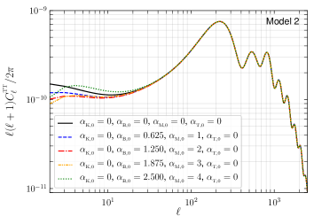
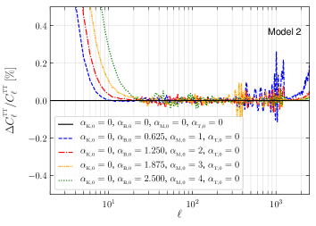
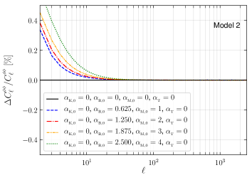
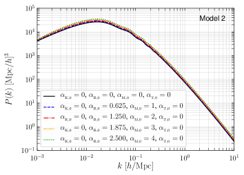
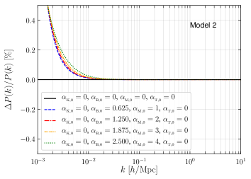
Figure 1: Comparison for the spectra for model 2 ($f(R)$-like). In the left hand panels we present the spectra obtained with EoS_class| and on the right the relative difference with the spectra of model 5 with $\alpha_{\rm K,0}=1$, as explained in the text. Top panels show the angular temperature anisotropy power spectrum, middle panels the angular power spectrum of the lensing potential, while bottom panels present the linear matter power spectrum. The black solid line represents the model with $\alpha_{\rm B,0}=\alpha_{\rm M,0}=0$, the dashed blue (red dot-dashed) stands for $\alpha_{\rm B,0}=0.625$ and $\alpha_{\rm M,0}=1$ ($\alpha_{\rm B,0}=1.25$ and $\alpha_{\rm M,0}=2$), the orange dot-dotted-dashed (dotted green) curve is for $\alpha_{\rm B,0}=1.875$ and $\alpha_{\rm M,0}=3$ ($\alpha_{\rm B,0}=2.5$ and $\alpha_{\rm M,0}=4$), respectively. For all the models, $\alpha_{\rm K,0}=0$.

4 Code validation

In this section we compare spectra obtained with our code EoS_class with results from hi_class. We compute the dimensionless CMB angular temperature anisotropy power spectra $C_{\ell}^{\rm TT}$, the dimensionless angular power spectrum of the lensing potential $C_{\ell}^{\phi\phi}$ and the total linear matter power spectrum $P(k)$ in units (Mpc/$h$)³.

We do not report here a similar comparison with EFTCAMB, as a detailed analysis for Horndeski models between these two codes has already been done in [55]. Note that in [55] we had also demonstrated the accuracy of our implementation of the EoS approach for $f(R)$ models compared to EFTCAMB.

In Figs. 2–5 we present the comparison for models 3–6, respectively. Model 1, that corresponds to setting $\alpha_{\rm B}=\alpha_{\rm M}=\alpha_{\rm T}=0$ and $\alpha_{\rm K}\neq 0$, is shown as the black lines on Figs. 2–5. In the right hand panels we show the relative difference $\Delta C/C$, with $C=\{C_{\ell}^{\rm TT},C_{\ell}^{\phi\phi},P(k)\}$ and $\Delta C\equiv C^{\verb|EoS_class|}-C^{\verb|hi_class|}$ and in the denominator we use $C=C^{\verb|EoS_class|}$. In each figure we have chosen a set of five specific values for the $\alpha_{\rm x}$s, the same values that were used for the hi_class paper in [47].

For all the models we considered, we achieve sub-percent agreement with the hi_class results. Since hi_class does not work for model 2 ($f(R)$-like models), we could not compare our results with hi_class for this class of models. Instead, in Fig. 1, we compare model 2 with model 5 with the same parameters, except $\alpha_{\rm K,0}=1$. Indeed, the only difference between both classes of models is that in model 5 $\alpha_{\rm K}\neq 0$. In this figure, $\Delta C=C^{\rm Model\leavevmode\nobreak\ 2}-C^{\rm Model\leavevmode\nobreak\ 5}$ and in the denominator $C=C^{\rm Model\leavevmode\nobreak\ 2}$. From this figure, we see that $\alpha_{\rm K}$ plays a role only for the largest cosmological scales with $k\lesssim 10^{-2}\leavevmode\nobreak\ h/{\rm Mpc}$, or $\ell\lesssim 10$. This result has also been found in [95], where the authors showed that $\alpha_{\rm K}$ only affects low multipoles in the ISW tail and that the effect is not measurable since it is smaller than cosmic variance.

While we get sub-percent agreement with hi_class ($<0.1\%$ in almost all the cases), we note that the largest differences between hi_class and EoS_class arise for the temperature anisotropy power spectrum at $\ell\gtrsim 1000$. In fact we identified the source of this difference to be associated with the different versions of the CLASS code: hi_class is based on CLASS version 2.4.5, while for EoS_class we used a more recent version (2.6.3). Hence, we conclude that our implementation reproduces the results of hi_class for models 1 and 3–6 to high precision and appears to also be working for model 2.

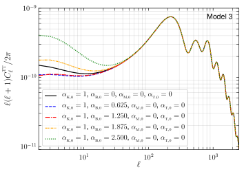
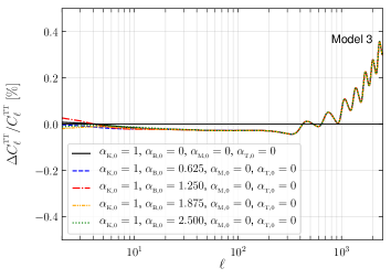
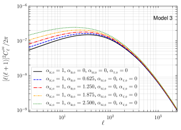
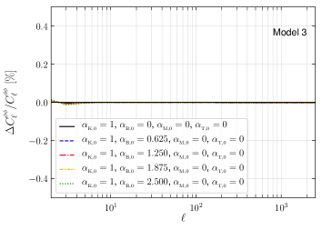
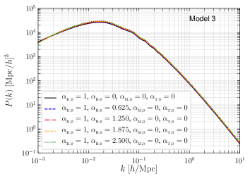
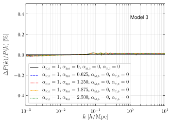
Figure 2: Comparison for the spectra for model 3 (KGB-like). In the left hand panels we present the spectra obtained with EoS_class| and on the right the relative difference with the corresponding spectra obtained with hi_class|. Top panels show the angular temperature anisotropy power spectrum, middle panels the angular power spectrum of the lensing potential, while bottom panels present the linear matter power spectrum. The black solid line represents the model with $\alpha_{\rm B,0}=0$, the dashed blue (red dot-dashed) stands for $\alpha_{\rm B,0}=0.625$ ($\alpha_{\rm B,0}=1.25$), the orange dot-dotted-dashed (dotted green) curve is for $\alpha_{\rm B,0}=1.875$ ($\alpha_{\rm B,0}=2.5$), respectively. For all the models, $\alpha_{\rm K,0}=1$.

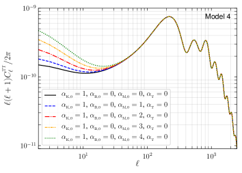
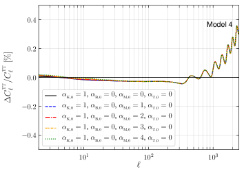
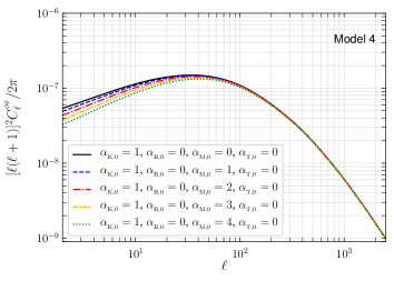
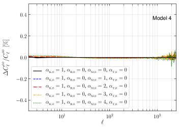
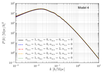
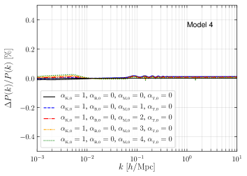
Figure 3: Comparison for the spectra for model 4. In the left hand panels we present the spectra obtained with EoS_class| and on the right the relative difference with the corresponding spectra obtained with hi_class|. Top panels show the angular temperature anisotropy power spectrum, middle panels the angular power spectrum of the lensing potential, while bottom panels present the linear matter power spectrum. The black solid line represents the model with $\alpha_{\rm M,0}=0$, the dashed blue (red dot-dashed) stands for $\alpha_{\rm M,0}=1$ ($\alpha_{\rm M,0}=2$), the orange dot-dotted-dashed (dotted green) curve is for $\alpha_{\rm M,0}=3$ ($\alpha_{\rm M,0}=4$), respectively. For all the models, $\alpha_{\rm K,0}=1$.

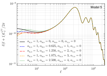
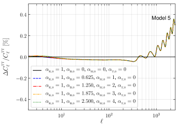
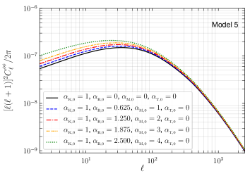
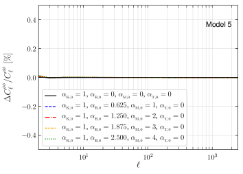
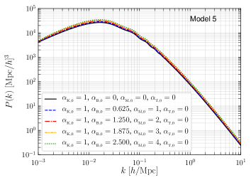
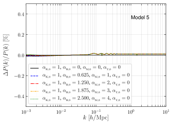
Figure 4: Comparison for the spectra for model 5. In the left hand panels we present the spectra obtained with EoS_class| and on the right the relative difference with the corresponding spectra obtained with hi_class|. Top panels show the angular temperature anisotropy power spectrum, middle panels the angular power spectrum of the lensing potential, while bottom panels present the linear matter power spectrum. The black solid line represents the model with $\alpha_{\rm B,0}=\alpha_{\rm M,0}=0$, the dashed blue (red dot-dashed) stands for $\alpha_{\rm B,0}=0.625$ and $\alpha_{\rm M,0}=1$ ($\alpha_{\rm B,0}=1.25$ and $\alpha_{\rm M,0}=2$), the orange dot-dotted-dashed (dotted green) curve is for $\alpha_{\rm B,0}=1.875$ and $\alpha_{\rm M,0}=3$ ($\alpha_{\rm B,0}=2.5$ and $\alpha_{\rm M,0}=4$), respectively. For all the models, $\alpha_{\rm K,0}=1$.

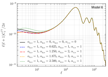
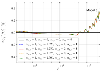
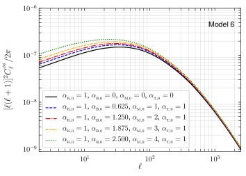
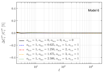
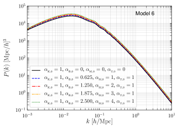
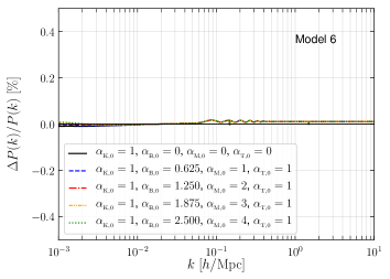
Figure 5: Comparison for the spectra for model 6. In the left hand panels we present the spectra obtained with EoS_class| and on the right the relative difference with the corresponding spectra obtained with hi_class|. Top panels show the angular temperature anisotropy power spectrum, middle panels the angular power spectrum of the lensing potential, while bottom panels present the linear matter power spectrum. The black solid line represents the model with $\alpha_{\rm B,0}=\alpha_{\rm M,0}=0$, the dashed blue (red dot-dashed) stands for $\alpha_{\rm B,0}=0.625$ and $\alpha_{\rm M,0}=1$ ($\alpha_{\rm B,0}=1.25$ and $\alpha_{\rm M,0}=2$), the orange dot-dotted-dashed (dotted green) curve is for $\alpha_{\rm B,0}=1.875$ and $\alpha_{\rm M,0}=3$ ($\alpha_{\rm B,0}=2.5$ and $\alpha_{\rm M,0}=4$), respectively. All the models have $\alpha_{\rm T,0}=1$. For all the models, $\alpha_{\rm K,0}=1$.

5 Dark sector evolution in Horndeski theories: analytical results

In this section we carry out an analytical analysis of Horndeski theories. In subsection 5.1 we present our analytical approximation for the attractor solution of the dark sector fluid variables. In subsection 5.2 we present new expressions for the standard modified gravity parameters for cosmological perturbations: $\mu$ (or $G_{\rm eff}$), $\eta$ and $\Sigma$. Finally, in subsection 5.3 we present simplified forms of the EoS for perturbations in Horndeski models.

5.1 Analytical approximations for the attractor solution

The existence of an attractor solution for the dark sector variables in modified gravity or dark energy models has been recognised and used in several previous analysis, for instance [96, 94, 48]. Here we derive an analytical approximation for the attractor solution of Horndeski theories. Our derivation relies on two single assumptions: that the mode as comoving wavelength is well inside the Hubble horizon, ${\rm K}^{2}\gg 1$, and that time derivatives can be neglected.

This assumption on the modes wavenumber determines the range of validity of our approximation in terms of scale. In fact, as can be seen in the top panel of Fig. 2 of [48], the condition ${\rm K}^{2}\gg 1$ translates into $k\gg 10^{-4}\leavevmode\nobreak\ {\rm Mpc}^{-1}$ today or $k\gg 10^{-3}\leavevmode\nobreak\ {\rm Mpc}^{-1}$ at $z\approx 100$. This includes the range of wavenumbers of observational interest, so this condition is not restrictive for our purposes.

This assumption also naturally implies that the gauge-invariant velocity perturbation $\hat{\Theta}$ is small compared to the gauge invariant density perturbation $\Delta$ in both the matter and dark sector. To see why this is the case, we write Einstein field equations in terms of the gauge-invariant quantities introduced in [63]

$$-\frac{2}{3}{\rm K}^{2}Z= \,\sum_{i}\Omega_{i}\Delta_{i}\,,$$ (5.1a)

$$2X= \,\sum_{i}\Omega_{i}\hat{\Theta}_{i}\,,$$ (5.1b)

$$\frac{1}{3}{\rm K}^{2}(Y-Z)= \,\sum_{i}\Omega_{i}w_{i}\Pi_{i}\,,$$ (5.1c)

where $Z$, $Y$ and $X$ on the left hand side are linear combinations of the metric perturbations and their derivatives with respect to $\ln{a}$, and the sum over $i$ on the right hand side means matter plus dark sector quantities. The different metric perturbations and their derivatives are generally all of the same order. Thus since ${\rm K}^{2}\gg 1$, we understand from Eqs. (5.1) that the gauge-invariant velocity perturbations are automatically smaller than the gauge-invariant density perturbations by a factor $\sim 1/{\rm K}^{2}$.

When we neglect velocity perturbations and take the derivative of Eqn. (3.3) we obtain

$$\Delta_{\rm ds}^{\prime\prime}+\left(2+3c_{\rm a,ds}^{2}-6w_{\rm ds}-\epsilon_{H}-2C_{\Pi\Delta_{\rm ds}}\right)\Delta_{\rm ds}^{\prime}+\left(c_{\rm a,ds}^{2}+C_{\zeta\Delta_{\rm ds}}\right){\rm K}^{2}\Delta_{\rm ds}=-\frac{\Omega_{\rm m}}{\Omega_{\rm ds}}C_{\zeta\Delta_{\rm m}}{\rm K}^{2}\Delta_{\rm m}\,,$$ (5.2)

where we replaced $\hat{\Theta}_{\rm ds}^{\prime}$ with Eqn. (3.4). Note that in this procedure, one has to initially keep terms proportional to ${\rm K}^{2}\hat{\Theta}_{\rm ds}$ since they are of the same order of magnitude as $\Delta_{\rm ds}$, when taking the derivative of Eqn. (3.3) and before additionally neglecting the contribution of velocity perturbations.

The differential equation for the density perturbation $\Delta_{\rm ds}$ (5.2) is similar to a damped harmonic oscillator sourced by matter perturbations. The time dependent frequency is $\omega^{2}=\left(c_{\rm a,ds}^{2}+C_{\zeta\Delta_{\rm ds}}\right){\rm K}^{2}\gg 1$ and is, in general, much smaller than the damping time scale represented by the Hubble expansion rate. This implies that the homogeneous solution becomes subdominant very quickly with respect to the particular solution, which, therefore, becomes the attractor of the evolution of the dark sector perturbations. In other words, similarly to what is normally done for the quasi-static approximation, we neglect the time derivatives of the density perturbation $\Delta_{\rm ds}$.

The analytical approximation for the attractor can be obtained by equating the last term of the left hand side with the term on the right hand side. This gives

$$\Delta_{\rm ds}=-\left(\frac{C_{\zeta\Delta_{\rm m}}}{c_{\rm a,ds}^{2}+C_{\zeta\Delta_{\rm ds}}}\right)\frac{\Omega_{\rm m}}{\Omega_{\rm ds}}\Delta_{\rm m}\;,$$ (5.3)

where in accordance to our definition of $w_{\rm ds}\zeta_{\rm ds}$ in Eqn. (3.5), $C_{\zeta\Delta_{i}}=\tfrac{2}{3}C_{\Pi\Delta_{i}}+C_{\Gamma\Delta_{i}}$, with $i=\{{\rm m},{\rm ds}\}$. Note that here we used the dimensionless perturbed fluid variables, not the tilde quantities. This expression generalises the one found in our previous paper [82] to non-constant $w_{\rm ds}$.

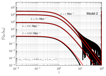
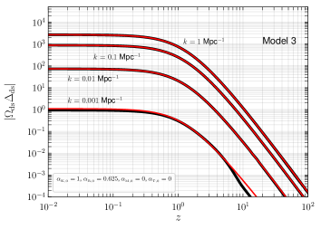
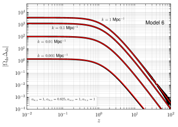
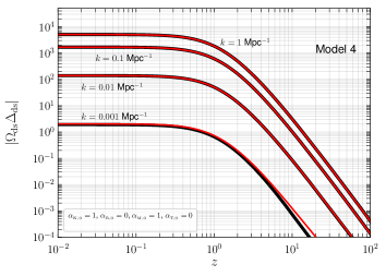
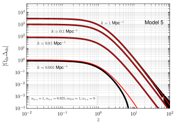
Figure 6: Evolution of the dark sector gauge invariant density perturbation $\Delta_{\rm ds}$ as a function of redshift $z$. The normalisation of the $\alpha$ functions is as follows: $\alpha_{\rm B,0}=0.625$, $\alpha_{\rm M,0}=1$ and $\alpha_{\rm T,0}=1$. From top left to bottom left, in clockwise order, we show the results for models 2–6, respectively. We consider four different wavelengths, $k=10^{-3}$ Mpc^-1, $k=10^{-2}$ Mpc^-1, $k=10^{-1}$ Mpc^-1 and $k=1$ Mpc^-1. The upper black solid lines represent the absolute value of $\Omega_{\rm ds}\Delta_{\rm ds}$ while the red lines on top of the black ones represent the attractor solution [Eqs. (5.3)]. For a wide range of $k$, the attractor approximation works well ($k\gtrsim 10^{-3}$Mpc^-1 at $z\lesssim 100$). Deviations between the numerical and analytical solution arise when ${\rm K}\sim 1$.

In Fig. 6 we present $\Omega_{\rm ds}\Delta_{\rm ds}$ as a function of redshift for four different scales and for models 2–6. We see that the attractor solution is manifestly a very good approximation of the numerical solution for scales $k\gtrsim 10^{-3}$Mpc^-1 at $z\lesssim 100$. For smaller scales, the attractor solution works well at low redshifts but only approximately for $z\gtrsim 1$ since the assumption ${\rm K}\sim 1$ is violated. The existence of an attractor and our analytical approximations allow us to derive several analytical results describing the properties of the dark sector, as we show in the next subsection.

5.2 New expressions for the Modified Gravity parameters in Horndeski models

A generic modified gravity model can either modify the Poisson equation or yield an anisotropic stress that leads to differences between the gravitational potentials (corresponding to $Z$ and $Y$ in our notation) or both at the same time. Hence, it is useful to recast the Einstein field equations in the following form

$$-\frac{2}{3}{\rm K}^{2}Z= \,\mu_{Z}({\rm K},a)\Omega_{\rm m}\Delta_{\rm m}\,,$$ (5.4a)

$$-\frac{2}{3}{\rm K}^{2}Y= \,\mu_{Y}({\rm K},a)\Omega_{\rm m}\Delta_{\rm m}\,,$$ (5.4b)

$$-\frac{2}{3}{\rm K}^{2}\Psi= \,\Sigma({\rm K},a)\Omega_{\rm m}\Delta_{\rm m}\,,$$ (5.4c)

$$\frac{Z}{Y}= \,\eta({\rm K},a)\,.$$ (5.4d)

In (5.4a) and (5.4b) the functions $\mu_{Z}$ and $\mu_{Y}$ parameterise the modifications to the Poisson equations for the gravitational potentials. In the conformal Newtonian gauge, $Z=\phi$ is the space-space component of the metric while $Y=\psi$ is the time-time component of the metric. Since $\mu_{Y}$ (often simply called $\mu$) is related to the time-time component of the metric and can therefore be seen as an effective modification of the Newton constant, it has also been called $G_{\rm eff}$ (or $G_{\rm matter}$) in previous works [97, 54]. Using Eqs. (5.1a) and (5.1c) together with Eqs. (5.4), these two functions, $\mu_{Z}$ and $\mu_{Y}$, can be written in terms of the perturbed fluid variables as

$$\mu_{Z}= \,1+\frac{\Omega_{\rm ds}\Delta_{\rm ds}}{\Omega_{\rm m}\Delta_{\rm m}}\,,$$ (5.5)

$$\mu_{Y}= \,\mu_{Z}-2\frac{\Omega_{\rm ds}w_{\rm ds}\Pi_{\rm ds}}{\Omega_{\rm m}\Delta_{\rm m}}\,.$$ (5.6)

In (5.4c) the function $\Sigma$ parameterises the departure of the lensing (Weyl) potential $\Psi\equiv(Z+Y)/2$ from its GR equivalent. It is related to the other functions via

$$\Sigma=\frac{1}{2}\left(\mu_{Z}+\mu_{Y}\right)=\frac{1}{2}\mu_{Y}\left(1+\eta\right)\,.$$ (5.7)

In previous works, $\Sigma$ has also been called $G_{\rm light}$ [98]. In (5.4d), the function $\eta$ (dubbed $\gamma$ in [54, 99]) is the gravitational slip, not to be confused with the metric variable “$\eta$” of the synchronous gauge. It is related to the other functions via

$$\eta=\frac{\mu_{Z}}{\mu_{Y}}\,.$$ (5.8)

This specific parametrisation of deviations from GR with the functions $\mu_{Z}$, $\mu_{Y}$, $\eta$ and $\Sigma$ has been widely used in recent research on dark energy and modified gravity. See for instance [100] for current CMB constraints on these functions. Note that since there are only two metric potentials, only two of these four functions are necessary to characterise a particular model; the most common choices are ($\mu_{Y},\eta$) or $(\mu_{Y},\Sigma)$.

Here we present new analytical expressions for these four functions, based on the analytical approximation of the attractor solution of the previous section. By simply replacing $\Delta_{\rm ds}$ in Eqn. (5.5) by its attractor, see Eqn. (5.3), we get an expression for $\mu_{Z}$. Then we insert this expression into Eqn. (5.6) and write $w_{\rm ds}\Pi_{\rm ds}=C_{\Pi\Delta_{\rm ds}}\Delta_{\rm ds}+\tfrac{\Omega_{\rm m}}{\Omega_{\rm ds}}C_{\Pi\Delta_{\rm m}}\Delta_{\rm m}$ where in accordance to our previous discussion we neglect the velocities. Again we replace $\Delta_{\rm ds}$ by its attractor and get the expression for $\mu_{Y}$. Finally, we use these expressions for $\mu_{Z}$ and $\mu_{Y}$ to write $\eta$ and $\Sigma$. All together, these expressions read

$$\mu_{Z}= \,\frac{\mu_{Z,0}+\mu_{Z,\infty}\left({\rm K}/{\rm K}_{\ast}\right)^{2}}{1+\left({\rm K}/{\rm K}_{\ast}\right)^{2}}\,,$$ (5.9a)

$$\mu=\mu_{Y}= \,\frac{\mu_{Y,0}+\mu_{Y,\infty}\left({\rm K}/{\rm K}_{\ast}\right)^{2}}{1+\left({\rm K}/{\rm K}_{\ast}\right)^{2}}\,,$$ (5.9b)

$$\eta= \,\frac{\mu_{Z,0}+\mu_{Z,\infty}\left({\rm K}/{\rm K}_{\ast}\right)^{2}}{\mu_{Y,0}+\mu_{Y,\infty}\left({\rm K}/{\rm K}_{\ast}\right)^{2}}\,,$$ (5.9c)

$$\Sigma= \,\frac{\Sigma_{0}+\Sigma_{\infty}\left({\rm K}/{\rm K}_{\ast}\right)^{2}}{1+\left({\rm K}/{\rm K}_{\ast}\right)^{2}}\,,$$ (5.9d)

where

$${{\rm K}_{\ast}}^{2}\equiv\frac{\gamma_{1}(\gamma_{2}-\alpha_{\rm T}/3)}{\alpha_{\rm B}^{2}c_{\rm s}^{2}}\,,$$ (5.10)

and where the functions $\mu_{Z,0}$, $\mu_{Y,0}$ and $\Sigma_{0}$ represent the values in the limit ${\rm K}\rightarrow 0$ and are given by

$$\mu_{Z,0}\equiv\frac{\gamma_{2}-\gamma_{7}}{\gamma_{2}-\alpha_{\rm T}/3}\frac{1}{\bar{M}^{2}}\,,\quad\mu_{Y,0}\equiv\mu_{Z,0}(1+\alpha_{\rm T})\,,\quad\eta_{0}\equiv\frac{\mu_{Z,0}}{\mu_{Y,0}}=\frac{1}{1+\alpha_{\rm T}}\,,\quad\Sigma_{0}\equiv\frac{1}{2}\left(\mu_{Y,0}+\mu_{Z,0}\right)\,,$$

with

$$\bar{M}^{2}\equiv\frac{M^{2}}{M_{\rm pl}^{2}}\,.$$

The functions $\gamma_{1}$, $\gamma_{2}$ and $\gamma_{7}$ are given in Appendix C.

The functions $\mu_{Z,\infty}$, $\mu_{Y,\infty}$, $\eta_{\infty}$ and $\Sigma_{\infty}$ represent the corresponding values in the limit ${\rm K}\rightarrow\infty$ and are given by

$$\mu_{Z,\infty}=\frac{\alpha c_{\rm s}^{2}+2\alpha_{\rm B}[\alpha_{\rm B}(1+\alpha_{\rm T})+\alpha_{\rm T}-\alpha_{\rm M}]}{\alpha c_{\rm s}^{2}\bar{M}^{2}}\,,$$ (5.11a)

$$\mu_{Y,\infty}=\frac{\alpha c_{\rm s}^{2}(1+\alpha_{\rm T})+2[\alpha_{\rm B}(1+\alpha_{\rm T})+\alpha_{\rm T}-\alpha_{\rm M}]^{2}}{\alpha c_{\rm s}^{2}\bar{M}^{2}}\,,$$ (5.11b)

$$\eta_{\infty}=\frac{\mu_{Z,\infty}}{\mu_{Y,\infty}}=\frac{\alpha c_{\rm s}^{2}+2\alpha_{\rm B}[\alpha_{\rm B}(1+\alpha_{\rm T})+\alpha_{\rm T}-\alpha_{\rm M}]}{\alpha c_{\rm s}^{2}(1+\alpha_{\rm T})+2[\alpha_{\rm B}(1+\alpha_{\rm T})+\alpha_{\rm T}-\alpha_{\rm M}]^{2}}\,,$$ (5.11c)

$$\Sigma_{\infty}=\frac{\mu_{Z,\infty}+\mu_{Y,\infty}}{2}=\frac{\alpha c_{\rm s}^{2}(2+\alpha_{\rm T})+2[\alpha_{\rm B}(1+\alpha_{\rm T})+\alpha_{\rm T}-\alpha_{\rm M}][\alpha_{\rm B}(2+\alpha_{\rm T})+\alpha_{\rm T}-\alpha_{\rm M}]}{2\alpha c_{\rm s}^{2}\bar{M}^{2}}\,,$$ (5.11d)

where $\alpha=\alpha_{\rm K}+6\alpha_{\rm B}^{2}$. Note that $\alpha_{\rm K}$ does not appear in any of the expressions (5.11).

The expressions for $\mu_{Y,\infty}$ and $\eta_{\infty}$ have already been obtained in previous works using different formulations of the Effective Field Theory formalism. [54] (see Eqs. (139) and (140)) and [101] (see Eqs. (3.18) and (3.19)) used the $\alpha$s functions introduced in [53] while [51] (see Eq. (70)) provided the expression for $\mu_{Y,\infty}$ based on a different set of functions which represent the coefficients of the perturbed operators and are constructed only with background quantities in the case of $\alpha_{\rm T}=0$. We refer to Table 2 of [53] for a translation between the perturbed variables $\alpha_{\rm x}$ and those used in [51].

To our knowledge, a few other works have obtained expressions that attempt model the scale dependence of these functions in Horndeski theories. In [68] (see Eqs. (45) and (52)) the authors considered the equations of motion of the perturbed scalar field and applied the quasi-static approximation (i.e. neglected the time derivatives of the metric potentials and of the perturbed scalar field). The remaining terms were used to rewrite the resulting Poisson equation in terms of an effective gravitational constant $\mu$. [102] (see Eqs. (4.15) and (4.18)) used a similar approach to [68] by considering only terms with ${\rm K}^{2}\gg 1$ and neglecting time derivatives of the fields. [103] used the quasi-static approximation and arguments of locality and general covariance to provide a general expression for $\mu_{Y}$ and $\eta$ (see Eqs. (24) and (25)). As stated in [103], these expressions have the same form as those in [68]. See also Eqs. (19) and (20) of [98]. [101] (see Eqs. (3.7) and (3.8)) used a so-called semi-dynamical approach. To study the evolution of perturbations beyond the quasi-static regime on small scales, these authors introduce terms that take into account corrections from the perturbed velocities and time derivatives of the metric potentials determined at a pivot scale of choice. All these approaches have two assumptions in common: they are valid on small scales and a variant of the quasi-static approximation is applied. The first assumption implies that only terms multiplied by ${\rm K}^{2}$ are considered with respect to the others; the second is equivalent to neglecting time derivatives of the relevant quantities appearing in the equations considered. More formally, these two assumptions imply ${\rm K}^{2}|X|\gg\{|X^{\prime}|,|X^{\prime\prime}|\}$, where $X=\{Z,Y,\delta\phi,\Delta_{\rm ds}\}$, where the appropriate variables are considered according to the set of equations the quasi-static approximation is applied to. Here, $\delta\phi$ represents the perturbation of the scalar degree of freedom.

The large scale limit of the expressions in [68, 102, 103, 101] differs from each other and ours due to the different assumptions. We will perform a detailed comparison of the different formulae for the modified gravity functions $\mu$ and $\eta$ in a forthcoming paper.

In Table (LABEL:tab:DEphenomenology_infinity) we report the limiting values of the MG functions in the limit ${\rm K}\rightarrow\infty$, in $\Lambda$CDM and in the six classes of models described in subsection 2.3. We also added a line corresponding to the so-called “no slip” model of [90]. The “no slip” model is a particular class of models that have $\alpha_{\rm M}=\alpha_{\rm B}$, $\alpha_{\rm K}$ free and $\alpha_{\rm T}=0$ (they are actually a subclass of the class of model 5). Hence one finds that $\gamma_{7}=0$ in the “no slip” model and, as a consequence, $\eta_{\infty}=1$ (“no slip”) while the other modified gravity functions are equal to $1/\bar{M}^{2}$. Moreover in the Table we have added two additional columns corresponding to the functions $\gamma_{\infty}\equiv 1/\eta_{\infty}-1$ and $g_{\infty}\equiv\tfrac{\mu_{Z,\infty}-\mu_{Y,\infty}}{\mu_{Z,\infty}+\mu_{Y,\infty}}=\tfrac{\eta_{\infty}-1}{\eta_{\infty}+1}$ which were used in [104]. This latter quantity is very well constrained in the Solar System by the Cassini mission [105]. Their general expressions are:

$$\gamma_{\infty}= \,\frac{\alpha\alpha_{\rm T}c_{\rm s}^{2}+2[\alpha_{\rm B}(1+\alpha_{\rm T})+\alpha_{\rm T}-\alpha_{\rm M}][\alpha_{\rm B}\alpha_{\rm T}+\alpha_{\rm T}-\alpha_{\rm M}]}{\alpha c_{\rm s}^{2}+2\alpha_{\rm B}[\alpha_{\rm B}(1+\alpha_{\rm T})+\alpha_{\rm T}-\alpha_{\rm M}]}\,,$$ (5.12a)

$$g_{\infty}= \,-\frac{\alpha\alpha_{\rm T}c_{\rm s}^{2}+2[\alpha_{\rm B}(1+\alpha_{\rm T})+\alpha_{\rm T}-\alpha_{\rm M}][\alpha_{\rm B}\alpha_{\rm T}+\alpha_{\rm T}-\alpha_{\rm M}]}{\alpha c_{\rm s}^{2}(2+\alpha_{\rm T})+2[\alpha_{\rm B}(1+\alpha_{\rm T})+\alpha_{\rm T}-\alpha_{\rm M}][\alpha_{\rm B}(2+\alpha_{\rm T})+\alpha_{\rm T}-\alpha_{\rm M}]}\,.$$ (5.12b)

Finally we note that we chose to write our formulae for the modified gravity functions, Eqs. (5.9a)–(5.9d) using ${\rm K}_{\ast}^{2}$ defined in Eqn. (5.10). Phenomenologically, ${\rm K}_{\ast}$ represents the transition scale between two regimes, large (${\rm K}\rightarrow 0$) and small (${\rm K}\rightarrow\infty$) scales. Indeed with this notation the expressions look relatively simple and compact. However it is true that in this form, if, for instance $\gamma_{1}$ or $\alpha_{\rm B}$ are zero, the expressions become ill-defined. In such cases, one can still use our expressions, but need to multiply both the numerator and denominator by ${\rm K}_{\ast}^{2}$ and potentially $\alpha_{\rm B}^{2}c_{\rm s}^{2}$. In this way, the expressions are always well defined.

5.3 Simplified EoS for perturbations

In this subsection we are interested in finding simplified expressions for the entropy perturbations and anisotropic stress of the dark sector, as these functions constitute a way of characterising a dark sector theory, independent and complementary to the modified gravity parameters of the previous section.

First we give the simplified expressions for the EoS that we obtained thanks to the attractor solution. Second we go through each class of models of subsection 2.3 and provide formulae for the EoS considering only the leading terms.

As we explained in the previous section for ${\rm K}^{2}\gg 1$, velocity perturbations are subdominant compared to density perturbations. With this assumption, we were able to express the dark sector density perturbation in terms of the matter perturbation, using the attractor solution of Eqn. (5.3). Now we consider the EoS for perturbations for $w_{\rm ds}\Gamma_{\rm ds}$, $w_{\rm ds}\Pi_{\rm ds}$ and $w_{\rm ds}\zeta_{\rm ds}$ presented in Eqs. (3.3), (3.4) and (3.5), respectively. In these expressions we neglect the velocity perturbations of both matter and dark sector and use the attractor solution to replace one density perturbation in terms of the other. This gives

$$w_{\rm ds}\Gamma_{\rm ds} =\frac{\Omega_{\rm m}}{\Omega_{\rm ds}}\left\{c_{\rm a,ds}^{2}+\frac{\Gamma_{0}+\Gamma_{\infty}\left({\rm K}/{\rm K}_{\ast}\right)^{2}}{1+\left({\rm K}/{\rm K}_{\ast}\right)^{2}}\right\}\Delta_{\rm m}\,,$$ (5.13a)

$$=-\frac{c_{\rm a,ds}^{2}+\Gamma_{0}+(c_{\rm a,ds}^{2}+\Gamma_{\infty})\left({\rm K}/{\rm K}_{\ast}\right)^{2}}{1-\mu_{Z,0}+(1-\mu_{Z,\infty})\left({\rm K}/{\rm K}_{\ast}\right)^{2}}\Delta_{\rm ds}\,,$$

$$w_{\rm ds}\Pi_{\rm ds} =\frac{\Omega_{\rm m}}{\Omega_{\rm ds}}\left\{\frac{\Pi_{0}+\Pi_{\infty}\left({\rm K}/{\rm K}_{\ast}\right)^{2}}{1+\left({\rm K}/{\rm K}_{\ast}\right)^{2}}\right\}\Delta_{\rm m}\,,$$ (5.13b)

$$=-\frac{\Pi_{0}+\Pi_{\infty}\left({\rm K}/{\rm K}_{\ast}\right)^{2}}{1-\mu_{Z,0}+(1-\mu_{Z,\infty})\left({\rm K}/{\rm K}_{\ast}\right)^{2}}\Delta_{\rm ds}\,,$$

$$w_{\rm ds}\zeta_{\rm ds} =\frac{\Omega_{\rm m}}{\Omega_{\rm ds}}\left\{c_{\rm a,ds}^{2}+\frac{\zeta_{0}+\zeta_{\infty}\left({\rm K}/{\rm K}_{\ast}\right)^{2}}{1+\left({\rm K}/{\rm K}_{\ast}\right)^{2}}\right\}\Delta_{\rm m}\,,$$ (5.13c)

$$=-\frac{c_{\rm a,ds}^{2}+\zeta_{0}+(c_{\rm a,ds}^{2}+\zeta_{\infty})\left({\rm K}/{\rm K}_{\ast}\right)^{2}}{1-\mu_{Z,0}+(1-\mu_{Z,\infty})\left({\rm K}/{\rm K}_{\ast}\right)^{2}}\Delta_{\rm ds}\,,$$

where

$$\Gamma_{0}\equiv\mu_{Z,0}\left(\frac{\alpha_{\rm T}}{3}-c_{\rm a,ds}^{2}\right)\,,\quad\Gamma_{\infty}\equiv\frac{1}{3}[\mu_{Y,\infty}-\mu_{Z,\infty}(1+3c_{\rm a,ds}^{2})]\,,\quad\Pi_{0}\equiv\frac{1}{2}(\mu_{Z,0}-\mu_{Y,0})\,,\quad\Pi_{\infty}\equiv\frac{1}{2}(\mu_{Z,\infty}-\mu_{Y,\infty})\,.$$

We also deduce that

$$\zeta_{0}\equiv\frac{2}{3}\Pi_{0}+\Gamma_{0}\,,\quad\zeta_{\infty}\equiv\frac{2}{3}\Pi_{\infty}+\Gamma_{\infty}\,.$$

This enables us to define the equation-of-state parameter for perturbations in Horndeski theories, $w_{\Gamma}\equiv w_{\rm ds}\Gamma_{\rm ds}/\Delta_{\rm ds}$ and $w_{\Pi}\equiv w_{\rm ds}\Pi_{\rm ds}/\Delta_{\rm ds}$, and for future numerical implementation, $w_{\zeta}\equiv\tfrac{2}{3}w_{\Pi}+w_{\Gamma}$, given by

$$w_{\Gamma} =-\frac{w_{\rm ds}+\Gamma_{0}+(w_{\rm ds}+\Gamma_{\infty})\left({\rm K}/{\rm K}_{\ast}\right)^{2}}{1-\mu_{Z,0}+(1-\mu_{Z,\infty})\left({\rm K}/{\rm K}_{\ast}\right)^{2}}\,,$$ (5.14a)

$$w_{\Pi} =-\frac{\Pi_{0}+\Pi_{\infty}\left({\rm K}/{\rm K}_{\ast}\right)^{2}}{1-\mu_{Z,0}+(1-\mu_{Z,\infty})\left({\rm K}/{\rm K}_{\ast}\right)^{2}}\,,$$ (5.14b)

$$w_{\zeta} =-\frac{w_{\rm ds}+\zeta_{0}+(w_{\rm ds}+\zeta_{\infty})\left({\rm K}/{\rm K}_{\ast}\right)^{2}}{1-\mu_{Z,0}+(1-\mu_{Z,\infty})\left({\rm K}/{\rm K}_{\ast}\right)^{2}}\,.$$ (5.14c)

In a way similar to the new expressions for $\mu$ and $\eta$ one can use these expressions for $w_{\Pi}$ and $w_{\zeta}$ to solve the dynamics of perturbations in Horndeski models, as we will show in our next paper.

In each of the classes of models we can get simplified expressions for $w_{\rm ds}\Gamma_{\rm ds}$, $w_{\rm ds}\Pi_{\rm ds}$ and $w_{\rm ds}\zeta_{\rm ds}$ by neglecting the velocities (except model 4). Since in each class of models some $\alpha$s are zero (except in model 6), the expressions simplify considerably. In model 1 ($k$-essence), since only $\alpha_{\rm K}$ is different from zero, we obtain without any approximation

$$w_{\rm ds}\Gamma_{\rm ds}=\left(c_{\rm s}^{2}-c_{\rm a,ds}^{2}\right)\Delta_{\rm ds}\,,\quad w_{\rm ds}\Pi_{\rm ds}=0\,,\quad w_{\rm ds}\zeta_{\rm ds}=w_{\rm ds}\Gamma_{\rm ds}\,,$$ (5.15)

where $c_{\rm s}^{2}$ and $c_{\rm a,ds}^{2}$ are the perturbations and adiabatic sound speed. Note that for a $\Lambda$CDM background, $w_{\rm ds}\Gamma_{\rm ds}=\Delta_{\rm ds}$.

For model 2 ($f(R)$-like), we obtain

$$w_{\rm ds}\Gamma_{\rm ds} =\left\{c_{\rm s}^{2}-\frac{1}{3}\frac{\alpha_{\rm M}}{\alpha_{\rm B}}-c_{\rm a,ds}^{2}+\frac{{\rm M}_{f}^{2}}{{\rm K}^{2}}\right\}\Delta_{\rm ds}+$$

$$\quad\frac{\Omega_{\rm m}}{\Omega_{\rm ds}}\left\{\left(c_{\rm s}^{2}-\frac{1}{3}\frac{\alpha_{\rm M}}{\alpha_{\rm B}}+\frac{{\rm M}_{f}^{2}}{{\rm K}^{2}}\right)\left(1-\frac{1}{\bar{M}^{2}}\right)+\frac{1}{3}\left(\frac{\alpha_{\rm M}}{\alpha_{\rm B}}-1\right)\frac{1}{\bar{M}^{2}}\right\}\Delta_{\rm m}\,,$$ (5.16a)

$$w_{\rm ds}\Pi_{\rm ds} =\frac{1}{2}\frac{\alpha_{\rm M}}{\alpha_{\rm B}}\left[\Delta_{\rm ds}+\frac{\Omega_{\rm m}}{\Omega_{\rm ds}}\left(1-\frac{1}{\bar{M}^{2}}\right)\Delta_{\rm m}\right]\,,$$ (5.16b)

$$w_{\rm ds}\zeta_{\rm ds} =\left\{c_{\rm s}^{2}-c_{\rm a,ds}^{2}+\frac{{\rm M}_{f}^{2}}{{\rm K}^{2}}\right\}\Delta_{\rm ds}+\frac{\Omega_{\rm m}}{\Omega_{\rm ds}}\left\{\left(c_{\rm s}^{2}+\frac{{\rm M}_{f}^{2}}{{\rm K}^{2}}\right)\left(1-\frac{1}{\bar{M}^{2}}\right)+\frac{1}{3}\left(\frac{\alpha_{\rm M}}{\alpha_{\rm B}}-1\right)\frac{1}{\bar{M}^{2}}\right\}\Delta_{\rm m}\,,$$ (5.16c)

where ${\rm M}_{f}^{2}\equiv-\epsilon_{H}(\bar{\epsilon}_{H}/\epsilon_{H}+\alpha_{\rm M}/\alpha_{\rm B}-2)/\alpha_{\rm B}$ generalises the mass term for $f(R)$ models, see e.g. [48]. Note that by setting $\alpha_{\rm M}=2\alpha_{\rm B}$, $c_{\rm s}^{2}=1$ and $\bar{M}^{2}=1$, one recovers the approximate $f(R)$ expressions already obtained in [48].

For model 3, as well as models 4, 5 and 6, we further assume that the modes are subhorizon (${\rm K}^{2}\gg 1$) to derive the simplified EoS for perturbations. For model 3 we obtain

$$w_{\rm ds}\Gamma_{\rm ds}=\left(c_{\rm s}^{2}-c_{\rm a}^{2}\right)\Delta_{\rm ds}-2\frac{\alpha_{\rm B}^{2}}{\alpha}\frac{\Omega_{\rm m}}{\Omega_{\rm ds}}\Delta_{\rm m}\,,\quad w_{\rm ds}\Pi_{\rm ds}=0\,,\quad w_{\rm ds}\zeta_{\rm ds}=w_{\rm ds}\Gamma_{\rm ds}\,.$$ (5.17)

For $\alpha_{\rm B}=0$, we recover the expression in Eqn. (5.15).

For model 4, there is a subtlety because $C_{\Pi\Delta}=0$, so the leading terms in the anisotropic stress are proportional to the velocity perturbations. We obtain

$$w_{\rm ds}\Gamma_{\rm ds} =\left(c_{\rm s}^{2}-2\frac{\alpha_{\rm M}}{\alpha_{\rm K}}-c_{\rm a,ds}^{2}\right)\Delta_{\rm ds}+\left(c_{\rm s}^{2}-2\frac{\alpha_{\rm M}}{\alpha_{\rm K}}-c_{\rm a,m}^{2}\right)\left(1-\frac{1}{\bar{M}^{2}}\right)\Delta_{\rm m}$$ (5.18a)

$$w_{\rm ds}\Pi_{\rm ds} =\frac{1}{3}C_{\Pi\Theta}{\rm K}^{2}\left[\Theta_{\rm ds}+\frac{\Omega_{\rm m}}{\Omega_{\rm ds}}\left(1-\frac{1}{\bar{M}^{2}}\right)\Theta_{\rm m}\right]\,,$$ (5.18b)

$$w_{\rm ds}\zeta_{\rm ds} =\left(c_{\rm s}^{2}-2\frac{\alpha_{\rm M}}{\alpha_{\rm K}}-c_{\rm a,ds}^{2}\right)\Delta_{\rm ds}+\left(c_{\rm s}^{2}-2\frac{\alpha_{\rm M}}{\alpha_{\rm K}}-c_{\rm a,m}^{2}\right)\left(1-\frac{1}{\bar{M}^{2}}\right)\Delta_{\rm m}\,,$$ (5.18c)

where

$$C_{\Pi\Theta}=\frac{\alpha_{\rm M}}{2\alpha_{\rm M}-\alpha_{\rm K}c_{\rm s}^{2}}\,.$$ (5.19)

Even if $c^{2}_{\rm a,m}\approx 0$ for matter at late time, we kept this term for symmetry reasons with respect to the coefficient of $\Delta_{\rm ds}$.

For model 5 we obtain

$$w_{\rm ds}\Gamma_{\rm ds}= \left(c_{\rm s}^{2}-\frac{1}{3}\frac{\alpha_{\rm M}}{\alpha_{\rm B}}-c_{\rm a,ds}^{2}\right)\Delta_{\rm ds}+\frac{\Omega_{\rm m}}{\Omega_{\rm ds}}\left[\left(c_{\rm s}^{2}-\frac{1}{3}\frac{\alpha_{\rm M}}{\alpha_{\rm B}}\right)\left(1-\frac{1}{\bar{M}^{2}}\right)-\frac{2}{\bar{M}^{2}}\frac{\alpha_{\rm B}(\alpha_{\rm B}-\alpha_{\rm M})}{\alpha}\right]\Delta_{\rm m}\,,$$ (5.20a)

$$w_{\rm ds}\Pi_{\rm ds}= \frac{1}{2}\frac{\alpha_{\rm M}}{\alpha_{\rm B}}\left[\Delta_{\rm ds}+\frac{\Omega_{\rm m}}{\Omega_{\rm ds}}\left(1-\frac{1}{\bar{M}^{2}}\right)\Delta_{\rm m}\right]\,,$$ (5.20b)

$$w_{\rm ds}\zeta_{\rm ds}= \left(c_{\rm s}^{2}-c_{\rm a,ds}^{2}\right)\Delta_{\rm ds}+\frac{\Omega_{\rm m}}{\Omega_{\rm ds}}\left[c_{\rm s}^{2}\left(1-\frac{1}{\bar{M}^{2}}\right)-\frac{2}{\bar{M}^{2}}\frac{\alpha_{\rm B}(\alpha_{\rm B}-\alpha_{\rm M})}{\alpha}\right]\Delta_{\rm m}\,.$$ (5.20c)

Note that when $\alpha_{\rm M}=0$, we recover model 3, while for $\alpha_{\rm B}=\alpha_{\rm M}=0$, we recover model 1. We also note that the term $\alpha_{\rm M}/\alpha_{\rm B}=\alpha_{\rm M,0}/\alpha_{\rm B,0}$ becomes time independent for a particular functional form of the $\alpha$ functions, i.e. when they are all proportional to the same time-dependent function.

We finally consider model 6 for which none of the $\alpha$s are zero. Nevertheless the expressions simplify for ${\rm K}^{2}\gg 1$. We obtain

$$w_{\rm ds}\Gamma_{\rm ds} =(\gamma_{3}-c_{\rm a,ds}^{2})\Delta_{\rm ds}+\frac{\Omega_{\rm m}}{\Omega_{\rm ds}}\left[\gamma_{3}\left(1-\frac{1}{\bar{M}^{2}}\right)+\frac{\gamma_{7}}{\bar{M}^{2}}\right]\Delta_{\rm m}\,,$$ (5.21a)

$$w_{\rm ds}\Pi_{\rm ds} =-\frac{1}{2}\left\{\gamma_{8}\Delta_{\rm ds}+\frac{\Omega_{\rm m}}{\Omega_{\rm ds}}\left[\frac{\alpha_{\rm T}}{\bar{M}^{2}}+\gamma_{8}\left(1-\frac{1}{\bar{M}^{2}}\right)\right]\Delta_{\rm m}\right\}\,,$$ (5.21b)

$$w_{\rm ds}\zeta_{\rm ds} =(c_{\rm s}^{2}-c_{\rm a,ds}^{2})\Delta_{\rm ds}+\frac{\Omega_{\rm m}}{\Omega_{\rm ds}}\left[c_{\rm s}^{2}\left(1-\frac{1}{\bar{M}^{2}}\right)+\frac{\gamma_{7}-\alpha_{\rm T}/3}{\bar{M}^{2}}\right]\Delta_{\rm m}\,,$$ (5.21c)

where $\gamma_{3}$, $\gamma_{7}$ and $\gamma_{8}$ are defined in Appendix C.

We verified numerically that the simplified equations of state in Eqs. (5.16), (5.17), (5.18), (5.20) and (5.21) provide an excellent approximation to the full expressions. When we use the simplified EoS we obtain CMB anisotropy temperature power spectra that agree at the sub-percent level with the exact solutions down to $\ell\approx 10-20$. For the linear matter power spectrum we get sub-percent agreement for all scales with $k\gtrsim 10^{-2}$ Mpc^-1. We checked this for the numerically most challenging models, i.e. 2 and 4, with extreme values of $\alpha_{\rm x,0}$ such as $\alpha_{\rm B,0}=2.5$ and $\alpha_{\rm M,0}=4$. We leave a more detailed analysis of the simplified EoS to a forthcoming paper.

6 Phenomenology of Horndeski theories

6.1 Understanding numerical results for several cosmological observables

Using our novel code EoS_class we have computed the dimensionless CMB angular temperature anisotropy power spectra $C_{\ell}^{\rm TT}$, the dimensionless angular power spectrum of the lensing potential $C_{\ell}^{\phi\phi}$ and the total linear matter power spectrum $P(k)$ in units (Mpc/$h$)³, for the six classes of models of Section 2.3 and these are presented in the left hand panels of Figs. 1–5.

Let us first consider the global behaviour of $\alpha_{\rm K}$ across the models studied here. In model 2 ($f(R)$-like), $\alpha_{\rm K,0}=0$ while in all the other models $\alpha_{\rm K,0}=1$. More in detail, model 5 differs from model 2 only in terms of $\alpha_{\rm K}$ and we will be comparing these models and study the effect of the kineticity term on the observables. $\alpha_{\rm K}$ does not appear in the expressions for $\mu$ and $\gamma$ in the limit ${\rm K}\rightarrow\infty$, but it is present in the transition scale ${\rm K}_{\ast}$ via the function $\gamma_{1}$. Comparing Fig. 1 with Fig. 4, one realises that the $\alpha_{\rm K}$ is only important on very large scales ($\ell\lesssim 20$ for the CMB temperature anisotropy and lensing potential power spectra and $k\lesssim 10^{-2}\leavevmode\nobreak\ h{\rm Mpc}^{-1}$ for the matter power spectrum), when analysing the right hand panels in Fig.1.

The effects of modified gravity, for the particular models considered here, are typically not that visible in the matter power spectrum, they are more relevant in the CMB temperature anisotropy and lensing potential power spectra, therefore we will discuss them more in detail. In the following we will consider separately the effects of varying $\alpha_{\rm B}$ and $\alpha_{\rm M}$ to understand their global behaviour and translate this into the effects of varying $\mu=\mu_{Y}$.

The braiding term is responsible for the fifth force and for an enhancement of clustering. Increasing the value of $\alpha_{\rm B,0}$ leads to an excess of power on small scales for the matter power spectrum and on large scales for the angular power spectrum of the lensing potential. The temperature anisotropy power spectrum is affected on large scales via the Integrated Sachs-Wolfe (ISW) effect, which is usually reduced. An increase in the braiding translates into an increase of the effective gravitational constant $\mu$. Therefore, increasing $\mu$ leads to an increase of power in both $P(k)$ and $C_{\ell}^{\phi\phi}$.

The rate of running of the Planck mass $\alpha_{\rm M}$ introduces anisotropic stress. An increase in $\alpha_{\rm M}$ leads to an excess of power in the CMB temperature power spectrum on large scales (low multipoles) due to the ISW effect and at the same time to a deficit in power in the lensing potential power spectrum. An increase in $\alpha_{\rm M}$ leads to a decrease of $\mu$ and $\eta$ and as a consequence a decrease in $\Sigma$ and this explains the decrease of power in $C_{\ell}^{\phi\phi}$.

Model 2 is the class of $f(R)$-like models and has $\alpha_{\rm B}\neq 0$ and $\alpha_{\rm M}\neq 0$, while $\alpha_{\rm K}=\alpha_{\rm T}=0$. The condition $\alpha_{\rm B}\neq 0$ is characteristic of a modified Newton’s law or an effective gravitational constant. For model 2, it can be written as

$$\mu=\frac{G_{\rm eff}}{G_{\rm N}}=\frac{3{\rm M}_{f}^{2}+[3c_{\rm s}^{2}+(\alpha_{\rm M}/\alpha_{\rm B}-1)^{2}]{\rm K}^{2}}{3{\rm M}_{f}^{2}+3c_{\rm s}^{2}{\rm K}^{2}}\frac{1}{\bar{M}^{2}}\,.$$ (6.1)

The condition $\alpha_{\rm M}\neq 0$ implies a non-vanishing slip (anisotropic stress)

$$\eta=\frac{3{\rm M}_{f}^{2}+[3c_{\rm s}^{2}-(\alpha_{\rm M}/\alpha_{\rm B}-1)]{\rm K}^{2}}{3{\rm M}_{f}^{2}+[3c_{\rm s}^{2}+(\alpha_{\rm M}/\alpha_{\rm B}-1)^{2}]{\rm K}^{2}}\,.$$ (6.2)

Their phenomenology is similar to $f(R)$ models as can be seen comparing the results of the panels of the left column of Fig. 1 with the top panels Fig. 3 of [48].

In model 3 (KGB-like, $\alpha_{\rm K}\neq 0$ and $\alpha_{\rm B}\neq 0$) there is also a modification to Newton’s law because the braiding is present ($\alpha_{\rm B}\neq 0$), but there is no anisotropic stress because $\alpha_{\rm M}=\alpha_{\rm T}=0$. One finds that

$$\mu_{\infty}=\frac{G_{\rm eff}}{G_{\rm N}}=1+\frac{2\alpha_{\rm B}^{2}}{\alpha c_{\rm s}^{2}}\,,\quad\eta_{\infty}=1\,.$$ (6.3)

Spectra for model 3 are presented in Fig. 2 for $\alpha_{\rm K,0}=1$ and four non-zero values of $\alpha_{\rm B,0}$ between 0.625 and 2.5. We see that the large-scale power increases monotonically with $\alpha_{\rm B,0}$ for all the spectra. When compared to model 2, we see that the effect of the variation of the braiding is stronger for the lensing potential and the temperature anisotropy, but smaller for the linear matter power spectrum.

In model 4 ($\alpha_{\rm K}\neq 0$ and $\alpha_{\rm M}\neq 0$), although $\alpha_{\rm B}=0$, both $\mu$ and $\eta$ are non-trivial. One has

$$\mu_{\infty}=\frac{G_{\rm eff}}{G_{\rm N}}=\left(1+\frac{2\alpha_{\rm M}^{2}}{\alpha_{\rm K}c_{\rm s}^{2}}\right)\frac{1}{\bar{M}^{2}}\,,\quad\eta_{\infty}=\left(1+\frac{2\alpha_{\rm M}^{2}}{\alpha_{\rm K}c_{\rm s}^{2}}\right)^{-1}\,.$$ (6.4)

Spectra for model 4 are presented in the left panels of Fig. 3 for $\alpha_{\rm K,0}=1$ and $\alpha_{\rm M,0}=1-4$. On large scales, we see that the CMB temperature power spectrum increases with $\alpha_{\rm M,0}$, however the lensing potential power spectrum decreases. As explained above, this can be linked to the decrease of the modified gravity parameter $\Sigma$ at late times, as shown on the bottom panel of Fig. 9.

For model 5, only $\alpha_{\rm T}=0$, and therefore neither $\mu$ nor $\eta$ are trivial. However, as before we can still obtain simplified expressions for the MG parameters in the small scale regimes (${\rm K}^{2}\gg 1$) and neglecting velocity perturbations:

$$\mu_{\infty} =\frac{G_{\rm eff}}{G_{\rm N}}=\frac{1+2(\alpha_{\rm B}-\alpha_{\rm M})^{2}}{\alpha c_{\rm s}^{2}}\frac{1}{\bar{M}^{2}}\,,$$ (6.5)

$$\eta_{\infty} =\frac{\alpha c_{\rm s}^{2}+2\alpha_{\rm B}(\alpha_{\rm B}-\alpha_{\rm M})}{\alpha c_{\rm s}^{2}+2(\alpha_{\rm B}-\alpha_{\rm M})^{2}}\,,$$ (6.6)

with the slip the same as for model 2, as expected. Spectra for these models are presented on the left panel of Fig. 4 with $\alpha_{\rm K,0}=1$, and several values for the parameters $\alpha_{\rm B,0}$ and $\alpha_{\rm M,0}$.

Finally, model 6 is the most general Horndeski model with all the $\alpha$s different from zero. Therefore, one can not simplify further the modified gravity expressions beyond the forms presented in Eqn. (5.9), or Eqs. (5.11) in the small scale regime. Spectra for these models are presented on the left panel of Fig. 5 with $\alpha_{\rm K,0}=\alpha_{\rm T,0}=1$, and several values for the parameters $\alpha_{\rm B,0}$ and $\alpha_{\rm M,0}$. By comparing Fig. (4) with Fig. (5), where the only difference is $\alpha_{\rm T}\neq 0$, we see that $\alpha_{\rm T}$ plays a minor role. The only noticeable difference is in the ISW effect for $\ell<5$ of the CMB temperature anisotropy power spectrum (upper left panels).

As previously stated, we are aware that models with $\alpha_{\rm T}\neq 0$ are now excluded by gravitational waves observations [74, 75, 76]. We decided to present these numerical results to show the robustness of our numerical implementation.

6.2 The time evolution of the modified gravity parameters

The commonly used modified gravity parameters, $\mu$ (or the effective modified gravitational constant $G_{\rm eff}$), $\eta$ (the slip) and $\Sigma$ (or $G_{\rm light}$), as well as the dark sector sound speed $c_{\rm s}^{2}$ and the effective Planck mass $\bar{M}^{2}$, are particularly useful to study the phenomenology of perturbations in dark sector theories. These are also the parameters that will be subject to observational constraints by forthcoming large-scale-structure and galaxy surveys, e.g. LSST [106], Euclid [107].

One can understand why these parameters are useful by considering the equation of motion for the gauge invariant matter perturbation. Indeed, following the same procedure as in [48] (see Eqn. (19a)), one can obtain an evolution equation for the matter density perturbations sourced by the dark sector density perturbations (under the assumptions of negligible velocity perturbations that generally corresponds to the small scale regime, ${\rm K}^{2}\gg 1$, and is valid for the modes of observational interest). Then with $\mu(=\mu_{Y}=G_{\rm eff}/G_{\rm N})$ as defined in Eqn. (5.6) one can write:

$$\Delta_{\rm m}^{\prime\prime}+(2-\epsilon_{H})\Delta_{\rm m}^{\prime}-\frac{3}{2}\frac{G_{\rm eff}}{G_{\rm N}}\Omega_{\rm m}\Delta_{\rm m}=0\,,$$ (6.7)

where in each class of Horndeski models the effective gravitational constant takes the forms presented in the previous section. This equation has been used to study the dark sector phenomenology in a number of works, see e.g. [48] for $f(R)$ gravity and [30, 108, 109] for other classes of Horndeski theories. Here we present the redshift evolution of the modified gravity parameters in Horndeski theories. For simplicity we present the behaviour of these function for sub-horizon modes, ${\rm K}^{2}\gg 1$.

In Fig. 7 we present the sound speed of dark sector perturbations as a function of redshift for models 2–6 and for different sets of values for $\alpha_{\rm x,0}$. The sound speed is important because it enters both the expressions of $G_{\rm eff}$ and the slip $\eta$, see Eqs. (5.11b) and (5.11c). In particular we see that when $c_{\rm s}^{2}$ becomes large, $G_{\rm eff}$ and $\eta$ reduce to their $\Lambda$CDM limit and therefore one does not expect a modified gravity behaviour of the matter and metric perturbations. We see in Fig. 7 that the sound speed is typically large at early times. This is because the sound speed $c_{\rm s}^{2}$ is proportional to $1/\alpha$ and $\alpha\propto\Omega_{\rm ds}$ in these models.

We note that for $k$-essence-like models (Model 1), the sound speed is $c_{\rm s}^{2}=3(1+w_{\rm ds})/\alpha_{\rm K}$ which becomes zero for the $\Lambda$CDM background that we are assuming. This corresponds to the solid black line on Fig. 7. In this case, the correct procedure to obtain the modified gravity parameters is to first evaluate their expressions by equating $\alpha_{\rm x}=0$ and then by setting $c_{\rm s}^{2}$. Therefore one obtains $\mu=\eta=\Sigma=1$.

In the bottom right panel of Fig. 7 we also show the evolution with respect to redshift of the effective Planck mass $\bar{M}^{2}$. Since $\alpha_{\rm M}\equiv d\ln{\bar{M}^{2}}/d\ln{a}$, $\bar{M}^{2}$ is larger at late time for larger values of $\alpha_{\rm M,0}$.

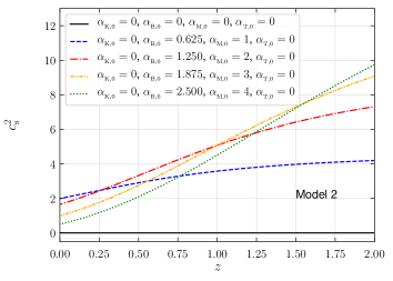
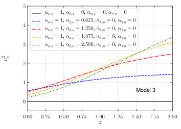
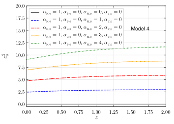
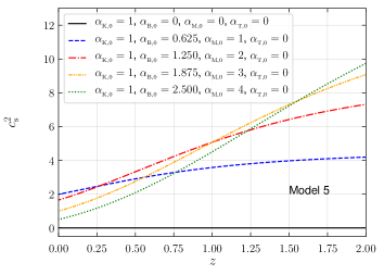
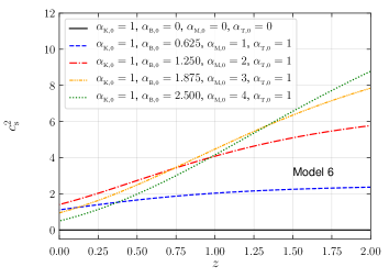
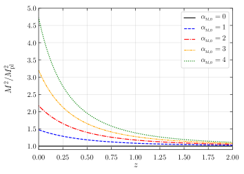
Figure 7: Evolution of the perturbation sound speed $c_{\rm s}^{2}$ for models 2–6 and for the effective Planck mass $\bar{M}^{2}=M^{2}/M_{\rm pl}^{2}$ for models 2 and 4–6. From left to right, in the top line we present the effective sound speed for models 2 and 3, in the middle line for models 4 and 5 and in the bottom line for model 6 and the effective Planck mass. Line styles and colours are as in Figs. 1–5 for models 2–6, respectively.

The effective gravitational constant $\mu_{Y}$ affects clustering and peculiar motion of galaxies while $\Sigma$ affects light geodesics. The first is constrained by galaxy clustering and redshift-space distortions [110, 111, 112], while the latter by the CMB, weak lensing and galaxy number counts [112, 113]. The parameters $\mu_{Y}$ and $\eta$ correspond to the parameters $Q$ and $R$ introduced in [97], respectively. We refer the reader to [97] for a comparison of different notations used in the literature.

In Figs. 8–11 we present the evolution of the modified gravity parameters $\mu_{Z}$, $\mu_{Y}$, $\eta$ and $\Sigma$ for the models 3–6. For simplicity we will consider only the values for ${\rm K}^{2}\gg 1$ and therefore we will not consider the scale dependence of this functions. Because of this choice, model 2 evolves identically to model 5 and we will not consider it further. We compared the full numerical solution obtained with our code EoS_class with the analytical expectation and found that they agree for $k\gtrsim 2\times 10^{-3}\leavevmode\nobreak\ h{\rm Mpc}^{-1}$. On larger scales, we see a departure of the analytical result from the full numerical solution, as the condition ${\rm K}^{2}\gg 1$ is violated. We will leave a detailed comparison of the analytical expressions with the exact numerical results in a forthcoming paper.

In Fig. 8 we present the time evolution of $\mu$ for model 3. In this class of models, the other modified gravity parameters are either trivial or identical to $\mu$. That is because $w_{\rm ds}\Pi_{\rm ds}=0$, i.e. $\eta=1$. We understand that $\mu$ increases at late times with increasing $\alpha_{\rm B}$ by looking at Eqn. (6.3) and by comparing with Fig. 2 we see that this increase of $\mu$ is associated with an amplification of matter clustering and ISW.

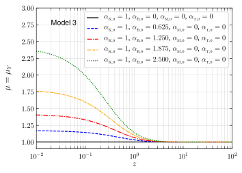
Figure 8: Evolution of the effective gravitational constant $\mu$ parameter for ${\rm K}^{2}\gg 1$ as a function of redshift $z$ for different values of the normalisation $\alpha_{\rm B,0}$ for model 3. Line styles and colours are as in Fig. 2. For this model, $\mu_{Z}=\mu_{Y}=\Sigma$ as $\eta=1$.

In Fig. 9 we present the time evolution of the modified gravity parameters for model 4 ($\mu_{Z}$, $\mu$, $\eta$ and $\Sigma$), for $\alpha_{\rm K,0}=1$ and different values of $\alpha_{\rm M,0}$. The functions $\mu_{Z}$, $\eta$ and $\Sigma$ become smaller than one and decrease at late times. The effect is more pronounced for larger values of $\alpha_{\rm M,0}$. For $\mu$, the effect is also more pronounced for larger values of $\alpha_{\rm M,0}$. Nevertheless the effect has a non-trivial time-dependence. In particular for all the values of $\alpha_{\rm M,0}$ considered, $\mu$ peaks at around $z\approx 0.7$, between 10 and 20% above the corresponding $\Lambda$CDM value ($\mu=1$). This different behaviour can be understood looking at the formula in Table LABEL:tab:DEphenomenology_infinity.

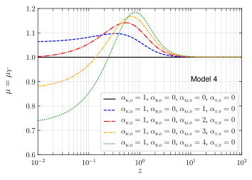
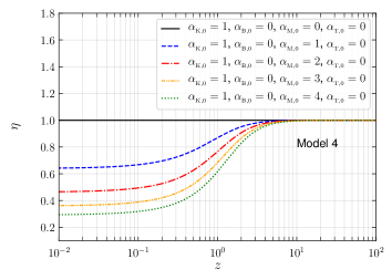
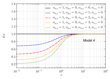
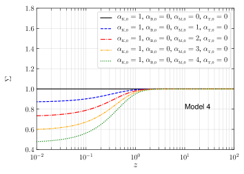
Figure 9: Evolution of the modified gravity parameters for ${\rm K}^{2}\gg 1$ as a function of redshift $z$ for the different values of $\alpha_{\rm M,0}$ for model 4. From top left in clockwise order we show $\mu$, $\eta$, $\Sigma$ and $\mu_{Z}$, respectively. Line styles and colours are as in Fig. 3.

Since $\alpha_{\rm T}$ plays a very minor role (at least for the value we considered, see discussion in Sect. 6.1), we discuss models 5 and 6 together. These models are the most general with $\alpha_{\rm K}$, $\alpha_{\rm B}$ and $\alpha_{\rm M}$ different from zero. The modified gravity functions for models 5 and 6 are shown in Figs. 10 and 11, respectively. We show the modified gravity functions for a different set of values of the $\alpha$s, with $\alpha_{\rm K,0}=1$ and four different values of $\alpha_{\rm B,0}$ between 0.625 and 2.5 and four different values of $\alpha_{\rm M,0}$ between 1 and 4. We see that $\mu$ and $\Sigma$ depart from unity and increase at late times. Meanwhile, $\mu_{Z}$ and $\eta$ decrease in a similar way as model 4. Hence, comparing with model 4, we can say that $\alpha_{\rm M}$ plays a more important role than $\alpha_{\rm B}$ for $\Sigma$ and $\mu_{Z}$. Moreover, we can say that $\alpha_{\rm B}$ plays a more important role than $\alpha_{\rm M}$ for $\mu$ and $\Sigma$. Again, this can be understood looking at the expressions in Table LABEL:tab:DEphenomenology_infinity. In particular, by noticing the effect of the effective Planck mass $\bar{M}^{2}$ on these functions. The increase of $\Sigma$ can be linked with the increase of the lensing potential in Fig. 4 and 5.

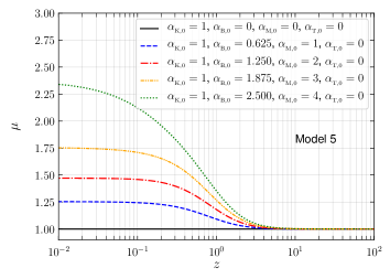
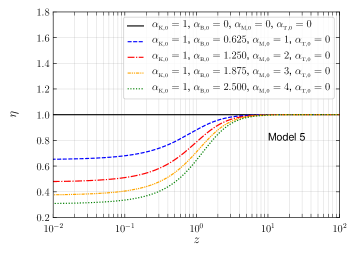
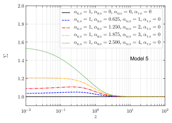
Figure 10: Evolution of the modified gravity parameters for ${\rm K}^{2}\gg 1$ as a function of redshift $z$ for the different values of $\alpha_{\rm B,0}$ and $\alpha_{\rm M,0}$ for model 5. From top left in clockwise order we show $\mu$, $\eta$, $\Sigma$ and $\mu_{Z}$, respectively. Line styles and colours are as in Fig. 4.

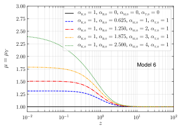
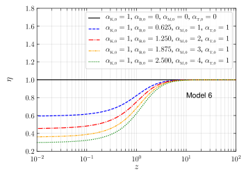
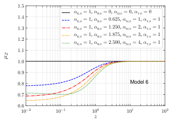
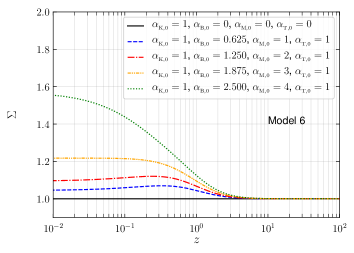
Figure 11: Evolution of the modified gravity parameters for ${\rm K}^{2}\gg 1$ as a function of redshift $z$ for the different values of $\alpha_{\rm B,0}$ and $\alpha_{\rm M,0}$ at fixed $\alpha_{\rm T,0}=1$ for model 6. From top left in clockwise order we show $\mu$, $\eta$, $\Sigma$ and $\mu_{Z}$, respectively. Line styles and colours are as in Fig. 5.

6.3 The growth index

The growth index is defined as $\gamma\equiv\ln{f}/\ln{\Omega_{\rm m}}$ where $f=\Delta_{\rm m}^{\prime}/\Delta_{\rm m}$ is the growth rate [see 114]. These quantities (or more precisely $\gamma$ and $f\sigma_{8}$) have a clear $\Lambda$CDM expectation and have already been measured from galaxy surveys and redshift space distortions (RSD) experiment [115]. For instance, in $\Lambda$CDM one expects a scale-independent $f\sigma_{8}$ and a constant growth index $\gamma=6/11$. With future surveys we will be able to determine with high significance whether these quantities match or depart from their $\Lambda$CDM expectation. It is therefore crucial to have clear understanding and predictions of the properties of the growth index and growth rate in modified gravity models and this can be done using expressions deduced in previous sections.

Here, we present the time evolution of the growth index in Horndeski theories. Taking the derivative of the growth rate, the equation describing the time evolution of the growth index is, e.g. [116, 48]

$$\gamma^{\prime}+\frac{3w_{\rm ds}\Omega_{\rm ds}}{\ln{\Omega_{\rm m}}}\gamma+\frac{\Omega_{\rm m}^{\gamma}}{\ln{\Omega_{\rm m}}}-\frac{3}{2}\frac{\Omega_{\rm m}^{1-\gamma}}{\ln{\Omega_{\rm m}}}\frac{G_{\rm eff}}{G_{\rm N}}=\frac{3w_{\rm ds}\Omega_{\rm ds}-1}{2\ln{\Omega_{\rm m}}}\;.$$ (6.8)

Since it is not possible to find an analytical solution to this equation, the standard procedure is to linearise it and assume that the early time solution holds also at later time when matter is no longer the dominant component, see [48] for details of the derivation of Eqn. (6.8) and its linearization. (Although [48] focuses on $f(R)$ gravity, the equations for the growth index, Eqs. (22)-(23) in that work apply to Horndeski models provided that $\epsilon$ is replaced by $G_{\rm eff}/G_{\rm N}$.) The solution can be found analytically only when $G_{\rm eff}/G_{\rm N}$ is approximately constant, which was the case for $f(R)$ models in [48] but is not generally true for the models we investigate here. Hence, we have to rely on numerical solutions.

We present our results for models 3–6 in Fig. 12. As in the previous section, we focus on the regime ${\rm K}^{2}\gg 1$. In all cases presented here, for all the different models, the effect of modified gravity decreases the growth index compared to its $\Lambda$CDM expectation (solid black lines in the figure). We note this is also the case in $f(R)$ gravity [48]. If the growth index is lower, it means that the growth rate, $f=\Omega_{\rm m}^{\gamma}$, is larger and therefore matter clustering is amplified. Hence in general one can expect an excess of power on small scales for the matter power spectrum $P(k)$. Nevertheless, one should also take into account another important aspect, namely the amount of time during which $\gamma$ remains significantly lower than the $\Lambda$CDM expectation value, as at early time all the models recover this value.

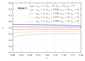
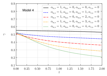
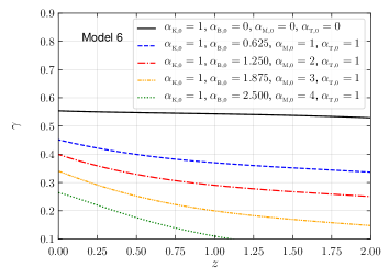
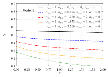
Figure 12: Time evolution for the growth index $\gamma$ for ${\rm K}^{2}\gg 1$. From top left in clockwise order we show models 3, 4, 5 and 6, respectively, Line styles and colours are as in Fig. 2, 3, 4, and 5, respectively.

6.4 The $E_{G}$ function

Zhang et al. (2007) [117] introduced the $E_{G}$ parameter as test for modified gravity and dark energy models. This quantity is defined as the ratio of the Laplacian of the Newtonian potentials to the peculiar velocity divergence. In our notation, using Einstein field equations, this quantity can be written as

$$E_{G}=\frac{\Omega_{\rm m,0}\Sigma}{\Delta_{\rm m}^{\prime}/\Delta_{\rm m}}\,,$$ (6.9)

where $\Sigma$, defined in Eqn. (5.4c), is proportional to the lensing (Weyl) potential and $\Delta_{\rm m}^{\prime}/\Delta_{\rm m}=\Omega_{\rm m}^{\gamma}$ is the growth rate discussed in the previous section. See also [81, 118] for recent updates on the measurability of the $E_{G}$ parameter.

Reyes et al. (2010) [119] were the first to measure $E_{G}$. They used galaxy-velocity cross-correlation and galaxy-galaxy lensing data from SDSS [120], and obtained a mean $E_{G}=0.39\pm 0.06$ (68%), at $z=0.32$ on small scales (${\rm K}^{2}\gg 1$). In $\Lambda$CDM, with $\Omega_{\rm m,0}=0.31$, we calculate $E_{G}^{\Lambda{\rm CDM}}=0.452\pm 0.029$ (68%) at $z=0.32$, where we quote the same uncertainty as [119]. The theoretical uncertainty is obtained by taking into account the error on the measure of $\Omega_{\rm m,0}$ and since we do not repeat the analysis of [119], we assume the same error bars. We note that our central $\Lambda$CDM value is substantially larger than the one quoted in [119]. This is because they assumed a lower value for $\Omega_{\rm m,0}$, namely $\Omega_{\rm m,0}=0.256\pm 0.018$ from WMAP 5-year data [121]. With our value of $\Omega_{\rm m,0}$, consistent with recent measurements [1], the value of $E_{G}$ measured by [119] is $\approx 1\sigma$ lower than the current $\Lambda$CDM value, although they are comparable within errors.

In Fig. 13 we present the redshift evolution of the $E_{G}$ parameter for Horndeski models 3–6 and the same values of the $\alpha_{\rm x,0}$ and cosmological parameters of Fig. 12 as used before in this work. We have included the $\Lambda$CDM expectation, namely $E_{G}^{\Lambda{\rm CDM}}=0.452\pm 0.029$ (68%), as the black point at $z=0.32$. Moreover, the solid black line shows the time evolution of $E_{G}$ for model 1 (Quintessence/$k$-essence) with only $\alpha_{\rm K}\neq 0$. For the value considered here ($\alpha_{\rm K,0}=1$), this model is indistinguishable from $\Lambda$CDM. In all the panels, we see that at early time ($z\gtrsim 1$), all the models give similar results as $\Lambda$CDM. Differences are most important for models 3 and 4 over a range of redshifts $z\lesssim 1.5$, while for models 5 and 6 differences are noticeable only at very low redshift $z\lesssim 0.3$.

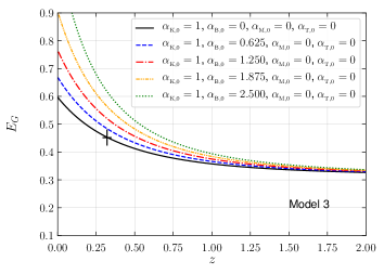
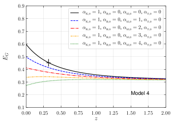
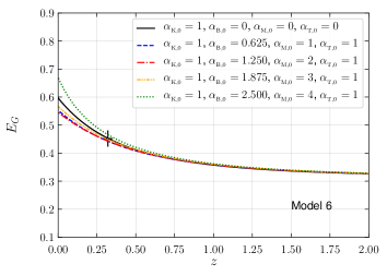
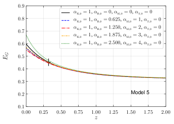
Figure 13: Time evolution for the quantity $E_{G}$. From top to bottom, we show models 3 to 6, respectively. Line style and colours are as in Fig. 2–5. The point with errorbars represent the expected value $E_{G}=0.452\pm 0.029$ for a $\Lambda$CDM model at $z=0.32$ with the cosmology assumed in this work. In agreement with the measurements of [119], for all the models we consider the value of $\Sigma_{\infty}$.

We see that for the models we have considered in our analysis, a measurement of $E_{G}$ with the uncertainty that we used (7% relative uncertainty) would not discriminate between the parameters used for models 5 and 6 and $\Lambda$CDM. However, it would exclude models 3 and 4 for $\alpha_{\rm B,0}\gtrsim 0.625$ and $\alpha_{\rm M,0}\gtrsim 1$. It would be interesting to update the measurements of $E_{G}$ with the latest galaxy survey data to check or revise these conclusions, with current and forecasted uncertainties.

We also note that this situation (the fact that some models are not discriminated by the $E_{G}$ statistics but are with the CMB temperature anisotropy power spectrum) is similar to what happens for $f(R)$ models, as shown in Fig. 4 (left panel) of [122]. Indeed, when $B_{0}\simeq 10$, the value of $E_{G}$ for $f(R)$ models is very close to the expectation value of the $\Lambda$CDM cosmology.

7 Conclusions

In this work we studied modifications to General Relativity corresponding to Horndeski theories [19, 20, 21]. Rather than using a scalar field or an Effective Field Theory approach, we have recast the Horndeski modifications as a dark energy fluid for both the background and the linear cosmological perturbations. Thus, we have extended the works of [63, 48, 91], and applied the EoS approach [59, 60, 61, 62] to the full Horndeski theories for the first time.

We have implemented the EoS approach for Horndeski into a modified version of the CLASS code [43, 44]. Our code, EoS_class, will be made publicly available online upon acceptance of this manuscript. Our code is as fast as hi_class [47] (an independent code for Horndeski theories based on the EFT approach [53]) for the models we studied. If we account for the different versions of CLASS used in EoS_class and hi_class, we get agreement with the latter within 0.1% relative error. Moreover, unlike hi_class, our code can solve the dynamics of cosmological perturbations in Horndeski models with $\alpha_{\rm K}=0$.

For sub-horizon modes, following a procedure similar to the quasi-static approximation where time derivatives are neglected, we have obtained an analytical approximation for the attractor solution of the gauge-invariant dark sector density perturbation. Using our analytical result, we derived new expressions for the modified gravity parameters, e.g. $\mu$, $\eta$ and $\Sigma$, that feature a scale dependence. Similar formulae had been obtained in previous works [68, 101, 102, 103, 98]. Although all the formulae for the modified gravity parameters agree in the small scale limit, they all differ in the large scale limit. Therefore, in a forthcoming paper, we will explicitly compare these formulae between them and with the exact numerical solution. The open question is: which one of the scale-dependent formulae for the modified gravity parameters has the widest range of validity when ${\rm K}^{2}=k^{2}/(aH)^{2}\ll 1$? Having an accurate analytical approximation of the modified gravity parameters is useful because it enables a simple implementation of modified gravity dynamics, which can be observationally tested, as well as a relatively simple phenomenological discussion.

With our exact numerical solutions computed with EoS_class and our analytical approximations of the modified gravity parameters we have studied the phenomenology of Horndeski models at the level of CMB temperature and lensing and matter power spectra as well as the growth index and the $E_{G}$ function of [117].

Appendix A Background expressions for Horndeski models

In this section we present explicit expressions for the background quantities describing Horndeski models.

The density $\rho_{\rm ds}$ and the pressure $P_{\rm ds}$ are, respectively [68, 69]

$$\rho_{\rm ds}= \,2XG_{2,X}-G_{2}-XG_{3,\phi}-6H\dot{\phi}XG_{3,X}-6H^{2}(G_{4}-4XG_{4,X}-4X^{2}G_{4,XX})-$$

$$\,6H\dot{\phi}(G_{4,\phi}+2XG_{4,\phi X})+2H^{3}\dot{\phi}X(5G_{5,X}+2XG_{5,XX})+3H^{2}X(3G_{5,\phi}+2XG_{5,\phi X})+$$

$$\,3H^{2}M_{\rm pl}^{2}\,,$$ (A.1)

$$P_{\rm ds}= \,G_{2}+X\left(2\ddot{\phi}G_{3,X}-G_{3,\phi}\right)+2\left(3H^{2}+2\dot{H}\right)G_{4}-4H\left(\dot{X}+3HX\right)G_{4,X}-$$

$$\,8X\left(\dot{H}G_{4,X}+H\dot{X}G_{4,XX}\right)+2\left(\ddot{\phi}+2H\dot{\phi}\right)G_{4,\phi}-2XG_{4,\phi\phi}+4\left(\ddot{\phi}-2H\dot{\phi}\right)XG_{4,\phi X}-$$

$$\,2X\left(2H^{3}\dot{\phi}+2H\dot{H}\dot{\phi}+3H^{2}\ddot{\phi}\right)G_{5,X}-4H^{2}\ddot{\phi}X^{2}G_{5,XX}-2HX\left(\dot{X}-HX\right)G_{5,\phi X}-$$

$$\,\left[2\left(HX\right)^{\hbox{$\cdot$}}+3H^{2}X\right]G_{5,\phi}-2H\dot{\phi}XG_{5,\phi\phi}-\left(3H^{2}+2\dot{H}\right)M_{\rm pl}^{2}\,.$$ (A.2)

The expressions relevant to the equation of motion of the scalar field are

$$J\equiv \,-2\dot{\phi}G_{2,X}-6HXG_{3,X}+2\dot{\phi}G_{3,\phi}-12H^{2}\dot{\phi}\left(G_{4,X}+2XG_{4,XX}\right)-12HXG_{4,\phi X}+$$

$$\,\phantom{-}2H^{3}X\left(3G_{5,X}+2XG_{5,XX}\right)-6H^{2}\dot{\phi}\left(G_{5,\phi}+XG_{5,\phi X}\right)\,,$$ (A.3)

$$P_{\phi}\equiv \,G_{2,\phi}-X\left(G_{3,\phi\phi}-2\ddot{\phi}G_{3,\phi X}\right)+6\left(2H^{2}+\dot{H}\right)G_{4,\phi}+6H\left(\dot{X}+2HX\right)G_{4,\phi X}+$$

$$\,3H^{2}XG_{5,\phi\phi}+2H^{3}\dot{\phi}XG_{5,\phi X}\;.$$ (A.4)

Appendix B Perturbation coefficients for Horndeski models

The perturbation coefficients, $\alpha_{\rm K}$, $\alpha_{\rm B}$, $\alpha_{\rm M}$ and $\alpha_{\rm T}$ in terms of the Horndeski functions $G_{i}$ are

$$M^{2} \equiv 2G_{4}-4XG_{4,X}-XG_{5,\phi}-2H\dot{\phi}XG_{5,X}\,,$$ (B.1)

$$H\alpha_{\rm M} \equiv \frac{d\ln{M^{2}}}{dt}\,,$$ (B.2)

$$M^{2}H^{2}\alpha_{\rm K} \equiv 2X\left(G_{2,X}+2XG_{2,XX}-G_{3,\phi}-XG_{3,\phi X}\right)$$ (B.3)

$$-12H\dot{\phi}X\left(G_{3,X}+XG_{3,XX}+3G_{4,\phi X}+2XG_{4,\phi XX}\right)$$

$$+12H^{2}X\left(G_{4,X}+8XG_{4,XX}+4X^{2}G_{4,XXX}\right)$$

$$+6H^{2}X\left(G_{5,\phi}+5XG_{5,\phi X}+2X^{2}G_{5,\phi XX}\right)$$

$$+4H^{3}\dot{\phi}X\left(3G_{5,X}+7XG_{5,XX}+2X^{2}G_{5,XXX}\right)\,,$$

$$2M^{2}H\alpha_{\rm B} \equiv 2\dot{\phi}X\left(G_{3,X}+2G_{4,\phi X}\right)+2\left(\frac{dG_{4}}{dt}-\frac{dX}{dt}G_{4,X}\right)$$ (B.4)

$$-4HX\left(2G_{4,X}+4XG_{4,XX}+G_{5,\phi}+XG_{5,\phi X}\right)$$

$$-2H^{2}\dot{\phi}X\left(3G_{5,X}+2XG_{5,XX}\right)\,,$$

$$\equiv 2\dot{\phi}\left(XG_{3,X}+G_{4,\phi}+2XG_{4,\phi X}\right)$$

$$-4HX\left(2G_{4,X}+4XG_{4,XX}+G_{5,\phi}+XG_{5,\phi X}\right)$$

$$-2H^{2}\dot{\phi}X\left(3G_{5,X}+2XG_{5,XX}\right)\,,$$

$$M^{2}\alpha_{\rm T} \equiv 2X\left[2G_{4,X}+G_{5,\phi}-\left(\ddot{\phi}-H\dot{\phi}\right)G_{5,X}\right]\,.$$ (B.5)

Note that evaluating $\alpha_{\rm M}$ as time derivative of $M^{2}$, rather than in terms of the derivatives of $G_{4}$ and $G_{5}$ with respect to $\phi$ and $X$ and $\alpha_{\rm B}$ in terms of the time derivative $G_{4}$ is more general since they allow to recover also results for $f(R)$ models.

Appendix C Coefficients for the EoS approach

In this section we provide the full expressions for the coefficients used in the EoS formalism. Having shown in [48] that the coefficients for the two gauge-invariant quantities $w_{\rm ds}\Gamma_{\rm ds}$ and $w_{\rm ds}\Pi_{\rm ds}$ lead to the same results for $f(R)$ models, here we generalise these expressions with the help of those provided by [54] in their Appendix C, Eqs. (184)-(195), for generic Horndeski models. As in [48], we used a standard continuity equation for the dark sector fluid which implies, for the background,

$$\rho_{\rm de}^{\rm GLV} =\rho_{\rm ds}+3(M^{2}-M_{\rm pl}^{2})H^{2}\;,$$

$$P_{\rm de}^{\rm GLV} =P_{\rm ds}-\left(3-2\epsilon_{H}\right)H^{2}(M^{2}-M_{\rm pl}^{2})\;,$$

where $\rho_{\rm de}^{\rm GLV}$ and $P_{\rm de}^{\rm GLV}$ are the variables used in [54] while $\rho_{\rm ds}$ and $P_{\rm ds}$ those used in this work; $M_{\rm pl}^{2}$ and $M^{2}$ are the standard and the effective Planck mass, respectively. Note that this also leads to a different background equation of state $w$ for the two conditions:

$$w_{\rm de}^{\rm GLV}=w_{\rm ds}+\frac{1}{3}\frac{2\epsilon_{H}-3(1+w_{\rm ds})}{\Omega_{\rm ds}+M^{2}/M_{\rm pl}^{2}-1}\left(\frac{M^{2}}{M_{\rm pl}^{2}}-1\right)\;,$$ (C.1)

where $\Omega_{\rm ds}$ represents the dark sector density parameter. The two agree only for minimally coupled models, i.e. when $M^{2}=M_{\rm pl}^{2}$. The background expressions are found by taking into account that $H$ is the same in both formalisms.

From now on, for compactness of the notation, we will define $\bar{M}^{2}\equiv M^{2}/M_{\rm pl}^{2}$.

For the perturbed variables, the relation between the variables in [54] and the ones adopted in our numerical implementation are:

$$\delta\rho_{\rm de}^{\rm GLV} =\bar{M}^{2}\delta\rho_{\rm ds}+\left(\bar{M}^{2}-1\right)\delta\rho_{\rm m}\;,$$

$$\delta P_{\rm de}^{\rm GLV} =\bar{M}^{2}\delta P_{\rm ds}+\left(\bar{M}^{2}-1\right)\delta P_{\rm m}\;,$$

$$q_{\rm m}^{\rm GLV}+q_{\rm de}^{\rm GLV} =-\bar{M}^{2}\frac{\bar{\rho}_{\rm ds}\hat{\Theta}_{\rm ds}+\bar{\rho}_{\rm m}\hat{\Theta}_{\rm m}}{3H}\;,$$

$$q_{\rm de}^{\rm GLV} =-\frac{1}{3H}\left[\bar{M}^{2}\bar{\rho}_{\rm ds}\hat{\Theta}_{\rm ds}+\left(\bar{M}^{2}-1\right)\bar{\rho}_{\rm m}\hat{\Theta}_{\rm m}\right]\;,$$

$$\sigma_{\rm m}^{\rm GLV}+\sigma_{\rm de}^{\rm GLV} =-\frac{a^{2}}{k^{2}}\bar{M}^{2}(\bar{P}_{\rm ds}\Pi_{\rm ds}+\bar{P}_{\rm m}\Pi_{\rm m})\;,$$

$$\sigma_{\rm de}^{\rm GLV} =-\frac{a^{2}}{k^{2}}\left[\bar{M}^{2}\bar{P}_{\rm ds}\Pi_{\rm ds}+\left(\bar{M}^{2}-1\right)\bar{P}_{\rm m}\Pi_{\rm m}\right]\;.$$

For $\bar{M}^{2}=1+f_{R}$, as it is the case in $f(R)$ models, we recover the expressions presented in [48]. We also made the following identifications: $q_{\rm m}^{\rm GLV}=-\frac{\rho_{\rm m}\Theta_{\rm m}}{3H}$ and $\sigma_{\rm m}^{\rm GLV}=-\tfrac{a^{2}}{k^{2}}P_{\rm m}\Pi_{\rm m}$. The relations between the perturbed expressions in the two formalisms are obtained by comparing the perturbed Einstein field equations.

With the help of the conversions reported above, we can now write the full expressions for the coefficients of the entropy perturbation $C_{\Gamma X}$ and anisotropic stress $C_{\Pi X}$, with $X=\Delta_{\rm ds,m}$, $\Theta_{\rm ds,m}$, $\Gamma_{\rm m}$ and $\Pi_{\rm m}$:

$$C_{\Gamma\Delta_{\rm ds}} \equiv\frac{\gamma_{1}\gamma_{2}+\tilde{\gamma}_{3}{\rm K}^{2}}{\gamma_{1}+\alpha_{\rm B}^{2}{\rm K}^{2}}-\frac{\mathrm{d}\bar{P}_{\rm ds}}{\mathrm{d}\bar{\rho}_{\rm ds}}\,,$$ (C.2)

$$C_{\Gamma\Theta_{\rm ds}} \equiv-\frac{1}{3}\frac{\gamma_{1}\gamma_{4}+\tilde{\gamma}_{5}{\rm K}^{2}}{\gamma_{1}+\alpha_{\rm B}^{2}{\rm K}^{2}}+\frac{\mathrm{d}\bar{P}_{\rm ds}}{\mathrm{d}\bar{\rho}_{\rm ds}}\,,$$ (C.3)

$$C_{\Gamma\Delta_{\rm m}} \equiv\frac{\gamma_{1}\gamma_{2}+\tilde{\gamma}_{3}{\rm K}^{2}}{\gamma_{1}+\alpha_{\rm B}^{2}{\rm K}^{2}}\left(1-\frac{1}{\bar{M}^{2}}\right)+\frac{\gamma_{7}}{\bar{M}^{2}}+\left(\frac{1}{\bar{M}^{2}}\frac{\alpha_{\rm K}}{\alpha}-1\right)\frac{\mathrm{d}\bar{P}_{\rm m}}{\mathrm{d}\bar{\rho}_{\rm m}}\,,$$ (C.4)

$$C_{\Gamma\Theta_{\rm m}} \equiv-\frac{1}{3}\left[\frac{\gamma_{1}\gamma_{4}+\tilde{\gamma}_{5}{\rm K}^{2}}{\gamma_{1}+\alpha_{\rm B}^{2}{\rm K}^{2}}\left(1-\frac{1}{\bar{M}^{2}}\right)+\frac{\gamma_{1}\gamma_{6}+3\tilde{\gamma}_{7}{\rm K}^{2}}{\gamma_{1}+\alpha_{\rm B}^{2}{\rm K}^{2}}\frac{1}{\bar{M}^{2}}+3\left(\frac{1}{\bar{M}^{2}}\frac{\alpha_{\rm K}}{\alpha}-1\right)\frac{\mathrm{d}\bar{P}_{\rm m}}{\mathrm{d}\bar{\rho}_{\rm m}}\right]\,,$$ (C.5)

$$C_{\Gamma\Gamma_{\rm m}} \equiv\frac{1}{\bar{M}^{2}}\frac{\alpha_{\rm K}}{\alpha}-1\,,$$ (C.6)

$$C_{\Pi\Delta_{\rm ds}} \equiv-\frac{1}{2}\frac{\gamma_{1}\alpha_{\rm T}+\tilde{\gamma}_{8}{\rm K}^{2}}{\gamma_{1}+\alpha_{\rm B}^{2}{\rm K}^{2}}\,,$$ (C.7)

$$C_{\Pi\Theta_{\rm ds}} \equiv\frac{1}{6}\frac{\gamma_{9}{\rm K}^{2}}{\gamma_{1}+\alpha_{\rm B}^{2}{\rm K}^{2}}\,,$$ (C.8)

$$C_{\Pi\Delta_{\rm m}} \equiv-\frac{1}{2}\left[\frac{1}{\bar{M}^{2}}\alpha_{\rm T}+\frac{\gamma_{1}\alpha_{\rm T}+\tilde{\gamma}_{8}{\rm K}^{2}}{\gamma_{1}+\alpha_{\rm B}^{2}{\rm K}^{2}}\left(1-\frac{1}{\bar{M}^{2}}\right)\right]\,,$$ (C.9)

$$C_{\Pi\Theta_{\rm m}} \equiv\frac{1}{6}\left[\frac{\gamma_{9}{\rm K}^{2}}{\gamma_{1}+\alpha_{\rm B}^{2}{\rm K}^{2}}\left(1-\frac{1}{\bar{M}^{2}}\right)+\frac{\gamma_{10}{\rm K}^{2}}{\gamma_{1}+\alpha_{\rm B}^{2}{\rm K}^{2}}\frac{1}{\bar{M}^{2}}\right]\,,$$ (C.10)

$$C_{\Pi\Pi_{\rm m}} \equiv-\left(1-\frac{1}{\bar{M}^{2}}\right)\,,$$ (C.11)

where, as before, ${\rm K}=\tfrac{k}{aH}$. Note that these coefficients refer to the dimensionful density and velocity perturbations and for clarity of notation we have used the labels $\Delta$ and $\Theta$ also for them. While this does not affect the coefficients for the dark sector variables, for the matter sector the coefficients for the dimensionless quantities differ by a factor $\Omega_{\rm m}(a)/\Omega_{\rm ds}(a)$ from the expressions above.

The $\gamma_{i}$ functions are given by:

$$\gamma_{1} \equiv\alpha_{\rm K}\frac{3\Omega_{\rm ds}(1+w_{\rm ds})-2\epsilon_{H}}{4\bar{M^{2}}}+\frac{1}{2}\alpha\epsilon_{H}\,,$$ (C.12)

$$\gamma_{2} \equiv c_{s}^{2}+\frac{\alpha_{\rm T}}{3}-2\frac{2\alpha_{\rm B}+\tilde{\Gamma}+(1+\alpha_{\rm B})(\alpha_{\rm M}-\alpha_{\rm T})}{\alpha}\,,$$ (C.13)

$$\gamma_{3} \equiv c_{\rm s}^{2}+\frac{\gamma_{8}}{3}\,,$$ (C.14)

$$\gamma_{4} \equiv\frac{1}{3\Omega_{\rm ds}(1+w_{\rm ds})+2\epsilon_{H}(\bar{M}^{2}-1)}\times$$

$$\quad\left\{9\Omega_{\rm ds}(1+w_{\rm ds})\frac{\alpha_{\rm K}}{\alpha}\frac{\mathrm{d}\bar{P}_{\rm ds}}{\mathrm{d}\bar{\rho}_{\rm ds}}+2(\epsilon_{H}-\bar{\epsilon}_{H})\left(\bar{M}^{2}-\frac{\alpha_{\rm K}}{\alpha}\right)-\right.$$

$$\qquad 3\alpha_{\rm M}(\Omega_{\rm m}+w_{\rm m}\Omega_{\rm m})+\left.\frac{18\alpha_{\rm B}}{\alpha}\left[\alpha_{\rm B}(3+\alpha_{\rm M})+\tilde{\Gamma}\right](\Omega_{\rm m}+w_{\rm m}\Omega_{\rm m})\right\}\,,$$ (C.15)

$$\gamma_{5} \equiv-1-\frac{(6\alpha_{\rm B}-\alpha_{\rm K})(\alpha_{\rm T}-\alpha_{\rm M})}{6\alpha_{\rm B}^{2}}+\frac{\alpha_{\rm B}^{2}}{\alpha}\left(\frac{\alpha_{\rm K}}{\alpha_{\rm B}^{2}}\right)^{\prime}\,,$$ (C.16)

$$\gamma_{6} \equiv\frac{\alpha_{\rm K}\alpha_{\rm M}-6\alpha_{\rm B}(3\alpha_{\rm B}+\tilde{\Gamma})}{\alpha}\,,$$ (C.17)

$$\gamma_{7} \equiv\frac{\alpha_{\rm K}\alpha_{\rm T}-6\alpha_{\rm B}(\alpha_{\rm B}+\alpha_{\rm T}-\alpha_{\rm M})}{3\alpha}\,,$$ (C.18)

$$\gamma_{8} \equiv\alpha_{\rm T}+\frac{\alpha_{\rm T}-\alpha_{\rm M}}{\alpha_{\rm B}}\,,$$ (C.19)

$$\gamma_{9} \equiv\frac{1}{2}\alpha(\alpha_{\rm T}-\alpha_{\rm M})\,,$$ (C.20)

$$\gamma_{10} \equiv 3\alpha_{\rm B}^{2}(\alpha_{\rm T}-\alpha_{\rm M})\,,$$ (C.21)

where the sound speed for the dark sector perturbations is given by

$$c_{\rm s}^{2}=-\frac{2(1+\alpha_{\rm B})[\alpha_{\rm B}(1+\alpha_{\rm T})-(\alpha_{\rm M}-\alpha_{\rm T})-\epsilon_{H}]+2\alpha_{\rm B}^{\prime}}{\alpha}-\frac{3(\Omega_{\rm m}+w_{\rm m}\Omega_{\rm m})}{\alpha\bar{M}^{2}}\,,$$ (C.22)

where $\Omega_{\rm m}=1-\Omega_{\rm ds}$ and $w_{\rm m}\Omega_{\rm m}=2\epsilon_{H}/3-1-w_{\rm ds}\Omega_{\rm ds}$.

For numerical convenience we also defined $\tilde{\gamma}_{i}=\alpha_{\rm B}^{2}\gamma_{i}$:

$$\tilde{\gamma}_{3} \equiv\alpha_{\rm B}^{2}c_{\rm s}^{2}+\frac{\tilde{\gamma}_{8}}{3}\,,$$ (C.23)

$$\tilde{\gamma}_{5} \equiv-\alpha_{\rm B}^{2}-\frac{(6\alpha_{\rm B}-\alpha_{\rm K})(\alpha_{\rm T}-\alpha_{\rm M})}{6}+\alpha_{\rm B}\frac{\alpha_{\rm K}^{\prime}\alpha_{\rm B}-2\alpha_{\rm K}\alpha_{\rm B}^{\prime}}{\alpha}\,,$$ (C.24)

$$\tilde{\gamma}_{8} \equiv\alpha_{\rm B}^{2}\alpha_{\rm T}+\alpha_{\rm B}(\alpha_{\rm T}-\alpha_{\rm M})\,.$$ (C.25)

These expressions are useful when $\alpha_{\rm B}=0$.

We further define $\gamma_{1}\tilde{\Gamma}=\alpha_{\rm B}\gamma_{1}\Gamma$

$$\gamma_{1}\tilde{\Gamma} \equiv \frac{\alpha_{\rm K}\alpha_{\rm B}}{4\bar{M}^{2}}\left[3(3+\alpha_{\rm M})(\Omega_{\rm m}+w_{\rm m}\Omega_{\rm m})+2(\epsilon_{H}-\bar{\epsilon}_{H})-9\Omega_{\rm ds}(1+w_{\rm ds})\frac{\mathrm{d}\bar{P}_{\rm ds}}{\mathrm{d}\bar{\rho}_{\rm ds}}\right]+$$ (C.26)

$$\frac{3\Omega_{\rm ds}(1+w_{\rm ds})+2\epsilon_{H}(\bar{M}^{2}-1)}{4\bar{M}^{2}}(\alpha_{\rm K}^{\prime}\alpha_{\rm B}-2\alpha_{\rm K}\alpha_{\rm B}^{\prime})-\frac{1}{2}\alpha\alpha_{\rm B}(4\epsilon_{H}-\bar{\epsilon}_{H})\,,$$

where $\epsilon_{H}=-\dot{H}/H^{2}=-H^{\prime}/H$ and $\bar{\epsilon}_{H}=-(\ddot{H}/H^{3}+4\dot{H}/H^{2})$. We further have $\bar{\epsilon}_{H}=\epsilon_{H}^{\prime}+4\epsilon_{H}-2\epsilon_{H}^{2}$.

It is also useful to consider the following coefficients

$$\gamma_{12} =\gamma_{1}\left[c_{\rm s}^{2}+\frac{\alpha_{\rm T}}{3}-2\frac{2\alpha_{\rm B}+(1+\alpha_{\rm B})(\alpha_{\rm M}-\alpha_{\rm T})}{\alpha}\right]-2\frac{\gamma_{1}\tilde{\Gamma}}{\alpha}\,,$$ (C.27)

$$\gamma_{14} =\frac{9\alpha_{\rm K}\Omega_{\rm ds}(1+w_{\rm ds})}{4\bar{M}^{2}}\frac{d\bar{P}_{\rm ds}}{d\bar{\rho}_{\rm ds}}-\frac{3\alpha_{\rm K}\alpha_{\rm M}(\Omega_{\rm m}+w_{\rm m}\Omega_{\rm m})}{4\bar{M}^{2}}+$$

$$\quad\frac{9(\Omega_{\rm m}+w_{\rm m}\Omega_{\rm m})}{2\alpha\bar{M}^{2}}\left(\alpha_{\rm K}^{\prime}\alpha_{\rm B}^{2}-2\alpha_{\rm K}\alpha_{\rm B}\alpha_{\rm B}^{\prime}\right)+\frac{1}{2}(\epsilon_{H}-\bar{\epsilon}_{H})\left(\alpha-\frac{\alpha_{\rm K}}{\bar{M}^{2}}\right)\,,$$ (C.28)

$$\gamma_{16} =\gamma_{1}\frac{\alpha_{\rm K}\alpha_{\rm M}-18\alpha_{\rm B}^{2}}{\alpha}-6\frac{\alpha_{\rm B}}{\alpha}\gamma_{1}\tilde{\Gamma}\,,$$ (C.29)

$$\gamma_{109} =\frac{1}{2}\alpha_{\rm K}(\alpha_{\rm M}-\alpha_{\rm T})\,,$$ (C.30)

where $\gamma_{12}\equiv\gamma_{1}\gamma_{2}$, $\gamma_{14}\equiv\gamma_{1}\gamma_{4}$, $\gamma_{16}\equiv\gamma_{1}\gamma_{6}$ and $\gamma_{109}\equiv\gamma_{10}-\gamma_{9}$. The first three are used in the code for models with $\alpha_{\rm B}\neq 0$.

Appendix D Precision parameters for the numerical solutions

In this section we report the precision parameters used in this work. For the comparison with results from the hi_class code, we adopted the same values used in [55], which we report here for completeness (see also their Appendix C). We note that one can generally get accurate spectra for less demanding values of the precision parameters.

 l_max_scalars = 5000
 P_k_max_h/Mpc = 12
 perturb_sampling_stepsize = 0.010
 tol_perturb_integration = 1e-10
 l_logstep = 1.045
 l_linstep = 25
 l_switch_limber = 20
 k_per_decade_for_pk = 200
 accurate_lensing = 1
 delta_l_max = 1000
 k_max_tau0_over_l_max = 8

References

- [1] Planck Collaboration VI, Planck 2018 results. VI. Cosmological parameters, ArXiv e-prints (July, 2018) , [1807.06209].
- [2] Planck Collaboration VIII, Planck 2018 results. VIII. Gravitational lensing, ArXiv e-prints (July, 2018) , [1807.06210].
- [3] Planck Collaboration X, Planck 2018 results. X. Constraints on inflation, ArXiv e-prints (July, 2018) , [1807.06211].
- [4] A. G. Riess, A. V. Filippenko, P. Challis and et al., Observational Evidence from Supernovae for an Accelerating Universe and a Cosmological Constant, AJ 116 (Sept., 1998) 1009–1038, [arXiv:astro-ph/9805201].
- [5] S. Perlmutter, G. Aldering, G. Goldhaber and et al., Measurements of Omega and Lambda from 42 High-Redshift Supernovae, APJ 517 (June, 1999) 565–586, [arXiv:astro-ph/9812133].
- [6] A. G. Riess, L.-G. Strolger, S. Casertano, H. C. Ferguson, B. Mobasher, B. Gold et al., New Hubble Space Telescope Discoveries of Type Ia Supernovae at z : Narrowing Constraints on the Early Behavior of Dark Energy, APJ 659 (Apr., 2007) 98–121, [arXiv:astro-ph/0611572].
- [7] S. Cole, W. J. Percival, J. A. Peacock, P. Norberg, C. M. Baugh, C. S. Frenk et al., The 2dF Galaxy Redshift Survey: power-spectrum analysis of the final data set and cosmological implications, MNRAS 362 (Sept., 2005) 505–534, [astro-ph/0501174].
- [8] M. A. Troxel, N. MacCrann, J. Zuntz, T. F. Eifler, E. Krause, S. Dodelson et al., Dark Energy Survey Year 1 Results: Cosmological Constraints from Cosmic Shear, ArXiv e-prints (Aug., 2017) , [1708.01538].
- [9] DES Collaboration, Dark Energy Survey year 1 results: Cosmological constraints from galaxy clustering and weak lensing, Phys. Rev. D 98 (Aug., 2018) 043526, [1708.01530].
- [10] D. Gruen, O. Friedrich, E. Krause, J. DeRose, R. Cawthon, C. Davis et al., Density split statistics: Cosmological constraints from counts and lensing in cells in DES Y1 and SDSS data, Phys. Rev. D 98 (July, 2018) 023507, [1710.05045].
- [11] S. Weinberg, The cosmological constant problem, Reviews of Modern Physics 61 (Jan., 1989) 1–23.
- [12] A. Joyce, B. Jain, J. Khoury and M. Trodden, Beyond the cosmological standard model, Physics Reports 568 (Mar., 2015) 1–98, [1407.0059].
- [13] A. Joyce, L. Lombriser and F. Schmidt, Dark Energy Versus Modified Gravity, Annual Review of Nuclear and Particle Science 66 (Oct., 2016) 95–122, [1601.06133].
- [14] K. Koyama, Cosmological tests of modified gravity, Reports on Progress in Physics 79 (Apr., 2016) 046902, [1504.04623].
- [15] M. Sami and R. Myrzakulov, Late-time cosmic acceleration: ABCD of dark energy and modified theories of gravity, International Journal of Modern Physics D 25 (Oct., 2016) 1630031.
- [16] J. Beltrán Jiménez, L. Heisenberg, G. J. Olmo and D. Rubiera-Garcia, Born-Infeld inspired modifications of gravity, Physics Reports 727 (Jan., 2018) 1–129, [1704.03351].
- [17] M. Ishak, Testing General Relativity in Cosmology, ArXiv e-prints (June, 2018) , [1806.10122].
- [18] L. Heisenberg, A systematic approach to generalisations of General Relativity and their cosmological implications, Physics Reports 796 (Mar, 2019) 1–113, [1807.01725].
- [19] G. W. Horndeski, Second-Order Scalar-Tensor Field Equations in a Four-Dimensional Space, International Journal of Theoretical Physics 10 (Sept., 1974) 363–384.
- [20] C. Deffayet, X. Gao, D. A. Steer and G. Zahariade, From k-essence to generalized Galileons, Phys. Rev. D 84 (Sept., 2011) 064039, [1103.3260].
- [21] T. Kobayashi, M. Yamaguchi and J. Yokoyama, Generalized G-Inflation — Inflation with the Most General Second-Order Field Equations —, Progress of Theoretical Physics 126 (Sept., 2011) 511–529, [1105.5723].
- [22] L. H. Ford, Cosmological-constant damping by unstable scalar fields, Phys. Rev. D 35 (Apr., 1987) 2339–2344.
- [23] P. J. E. Peebles and B. Ratra, Cosmology with a time-variable cosmological ’constant’, ApJL 325 (Feb., 1988) L17–L20.
- [24] B. Ratra and P. J. E. Peebles, Cosmological consequences of a rolling homogeneous scalar field, Phys. Rev. D 37 (June, 1988) 3406–3427.
- [25] C. Armendáriz-Picón, T. Damour and V. Mukhanov, k-Inflation, Physics Letters B 458 (July, 1999) 209–218, [hep-th/9904075].
- [26] V. Mukhanov and A. Vikman, Enhancing the tensor-to-scalar ratio in simple inflation, JCAP 2 (Feb., 2006) 4, [astro-ph/0512066].
- [27] C. Deffayet, O. Pujolàs, I. Sawicki and A. Vikman, Imperfect dark energy from kinetic gravity braiding, JCAP 10 (Oct., 2010) 026, [1008.0048].
- [28] O. Pujolàs, I. Sawicki and A. Vikman, The imperfect fluid behind kinetic gravity braiding, Journal of High Energy Physics 11 (Nov., 2011) 156, [1103.5360].
- [29] T. Kobayashi, M. Yamaguchi and J. Yokoyama, Inflation Driven by the Galileon Field, Phys. Rev. Lett. 105 (Dec., 2010) 231302, [1008.0603].
- [30] R. Kimura and K. Yamamoto, Large scale structures in the kinetic gravity braiding model that can be unbraided, JCAP 4 (Apr., 2011) 025, [1011.2006].
- [31] A. Silvestri and M. Trodden, Approaches to understanding cosmic acceleration, Reports on Progress in Physics 72 (Sept., 2009) 096901, [0904.0024].
- [32] T. P. Sotiriou and V. Faraoni, f(R) theories of gravity, Reviews of Modern Physics 82 (Jan., 2010) 451–497, [0805.1726].
- [33] A. De Felice and S. Tsujikawa, f( R) Theories, Living Reviews in Relativity 13 (Dec., 2010) 3, [1002.4928].
- [34] C. Brans and R. H. Dicke, Mach’s Principle and a Relativistic Theory of Gravitation, Physical Review 124 (Nov., 1961) 925–935.
- [35] N. Chow and J. Khoury, Galileon cosmology, Phys. Rev. D 80 (July, 2009) 024037, [0905.1325].
- [36] A. Nicolis, R. Rattazzi and E. Trincherini, Galileon as a local modification of gravity, Phys. Rev. D 79 (Mar., 2009) 064036, [0811.2197].
- [37] C. Deffayet, G. Esposito-Farèse and A. Vikman, Covariant Galileon, Phys. Rev. D 79 (Apr., 2009) 084003, [0901.1314].
- [38] S. M. Carroll, A. de Felice, V. Duvvuri, D. A. Easson, M. Trodden and M. S. Turner, Cosmology of generalized modified gravity models, Phys. Rev. D 71 (Mar., 2005) 063513, [astro-ph/0410031].
- [39] U. Seljak and M. Zaldarriaga, A Line-of-Sight Integration Approach to Cosmic Microwave Background Anisotropies, APJ 469 (Oct., 1996) 437, [astro-ph/9603033].
- [40] M. Kaplinghat, L. Knox and C. Skordis, Rapid Calculation of Theoretical Cosmic Microwave Background Angular Power Spectra, APJ 578 (Oct., 2002) 665–674, [astro-ph/0203413].
- [41] M. Doran, CMBEASY: an object oriented code for the cosmic microwave background, Journal of Cosmology and Astro-Particle Physics 10 (Oct., 2005) 11–+, [arXiv:astro-ph/0302138].
- [42] A. Lewis, A. Challinor and A. Lasenby, Efficient Computation of Cosmic Microwave Background Anisotropies in Closed Friedmann-Robertson-Walker Models, APJ 538 (Aug., 2000) 473–476, [arXiv:astro-ph/9911177].
- [43] J. Lesgourgues, The Cosmic Linear Anisotropy Solving System (CLASS) I: Overview, ArXiv e-prints (Apr., 2011) , [1104.2932].
- [44] D. Blas, J. Lesgourgues and T. Tram, The Cosmic Linear Anisotropy Solving System (CLASS). Part II: Approximation schemes, JCAP 7 (July, 2011) 034, [1104.2933].
- [45] B. Hu, M. Raveri, N. Frusciante and A. Silvestri, Effective field theory of cosmic acceleration: An implementation in CAMB, Phys. Rev. D 89 (May, 2014) 103530, [1312.5742].
- [46] M. Raveri, B. Hu, N. Frusciante and A. Silvestri, Effective field theory of cosmic acceleration: Constraining dark energy with CMB data, Phys. Rev. D 90 (Aug., 2014) 043513, [1405.1022].
- [47] M. Zumalacárregui, E. Bellini, I. Sawicki, J. Lesgourgues and P. G. Ferreira, hi_class: Horndeski in the Cosmic Linear Anisotropy Solving System, JCAP 8 (Aug., 2017) 019, [1605.06102].
- [48] R. A. Battye, B. Bolliet and F. Pace, Do cosmological data rule out f(R) with ?, Phys. Rev. D 97 (May, 2018) 104070, [1712.05976].
- [49] Z. Huang, A cosmology forecast toolkit — CosmoLib, JCAP 6 (June, 2012) 012, [1201.5961].
- [50] D. Traykova, E. Bellini and P. G. Ferreira, The phenomenology of beyond Horndeski gravity, arXiv e-prints (Feb., 2019) , [1902.10687].
- [51] G. Gubitosi, F. Piazza and F. Vernizzi, The effective field theory of dark energy, JCAP 2 (Feb., 2013) 032, [1210.0201].
- [52] J. Gleyzes, D. Langlois, F. Piazza and F. Vernizzi, Essential building blocks of dark energy, JCAP 8 (Aug., 2013) 025, [1304.4840].
- [53] E. Bellini and I. Sawicki, Maximal freedom at minimum cost: linear large-scale structure in general modifications of gravity, JCAP 7 (July, 2014) 050, [1404.3713].
- [54] J. Gleyzes, D. Langlois and F. Vernizzi, A unifying description of dark energy, International Journal of Modern Physics D 23 (Jan., 2014) 1443010, [1411.3712].
- [55] E. Bellini, A. Barreira, N. Frusciante, B. Hu, S. Peirone, M. Raveri et al., Comparison of Einstein-Boltzmann solvers for testing general relativity, Phys. Rev. D 97 (Jan., 2018) 023520, [1709.09135].
- [56] R. Arjona, W. Cardona and S. Nesseris, Unraveling the effective fluid approach for f (R ) models in the subhorizon approximation, Phys. Rev. D 99 (Feb., 2019) 043516, [1811.02469].
- [57] R. Arjona, W. Cardona and S. Nesseris, Designing Horndeski and the effective fluid approach, arXiv e-prints (Apr., 2019) , [1904.06294].
- [58] R. A. Battye and A. Moss, Cosmological perturbations in elastic dark energy models, Phys. Rev. D 76 (July, 2007) 023005, [astro-ph/0703744].
- [59] R. A. Battye and J. A. Pearson, Effective action approach to cosmological perturbations in dark energy and modified gravity, JCAP 7 (July, 2012) 019, [1203.0398].
- [60] R. A. Battye and J. A. Pearson, Parametrizing dark sector perturbations via equations of state, Phys. Rev. D 88 (Sept., 2013) 061301, [1306.1175].
- [61] R. A. Battye and J. A. Pearson, Massive gravity, the elasticity of space-time, and perturbations in the dark sector, Phys. Rev. D 88 (Oct., 2013) 084004, [1301.5042].
- [62] R. A. Battye and J. A. Pearson, Computing model independent perturbations in dark energy and modified gravity, JCAP 3 (Mar., 2014) 051, [1311.6737].
- [63] R. A. Battye, B. Bolliet and J. A. Pearson, f(R) gravity as a dark energy fluid, Phys. Rev. D 93 (Feb., 2016) 044026, [1508.04569].
- [64] C. Wetterich, Quintessence - the Dark Energy in the Universe?, Space Science Reviews 100 (Jan., 2002) 195–206, [arXiv:astro-ph/0110211].
- [65] C. Armendariz-Picon, V. Mukhanov and P. J. Steinhardt, Essentials of k-essence, Phys. Rev. D 63 (May, 2001) 103510, [arXiv:astro-ph/0006373].
- [66] S. M. Carroll, V. Duvvuri, M. Trodden and M. S. Turner, Is cosmic speed-up due to new gravitational physics?, Phys. Rev. D 70 (Aug., 2004) 043528, [astro-ph/0306438].
- [67] X. Gao, Conserved cosmological perturbation in Galileon models, JCAP 10 (Oct., 2011) 021, [1106.0292].
- [68] A. De Felice, T. Kobayashi and S. Tsujikawa, Effective gravitational couplings for cosmological perturbations in the most general scalar-tensor theories with second-order field equations, Physics Letters B 706 (Dec., 2011) 123–133, [1108.4242].
- [69] S. Nishi, T. Kobayashi, N. Tanahashi and M. Yamaguchi, Cosmological matching conditions and galilean genesis in Horndeski’s theory, JCAP 3 (Mar., 2014) 008, [1401.1045].
- [70] R. Kase and S. Tsujikawa, Dark energy in Horndeski theories after GW170817: A review, ArXiv e-prints (Sept., 2018) , [1809.08735].
- [71] I. Sawicki and E. Bellini, Limits of quasistatic approximation in modified-gravity cosmologies, Phys. Rev. D 92 (Oct., 2015) 084061, [1503.06831].
- [72] J. Gleyzes, D. Langlois, M. Mancarella and F. Vernizzi, Effective theory of dark energy at redshift survey scales, JCAP 2 (Feb., 2016) 056, [1509.02191].
- [73] D. Alonso, E. Bellini, P. G. Ferreira and M. Zumalacárregui, Observational future of cosmological scalar-tensor theories, Phys. Rev. D 95 (Mar., 2017) 063502, [1610.09290].
- [74] B. P. Abbott, R. Abbott, T. D. Abbott, F. Acernese, K. Ackley, C. Adams et al., GW170817: Observation of Gravitational Waves from a Binary Neutron Star Inspiral, Physical Review Letters 119 (Oct., 2017) 161101, [1710.05832].
- [75] B. P. Abbott, R. Abbott, T. D. Abbott, F. Acernese, K. Ackley, C. Adams et al., Gravitational Waves and Gamma-Rays from a Binary Neutron Star Merger: GW170817 and GRB 170817A, ApJL 848 (Oct., 2017) L13, [1710.05834].
- [76] B. P. Abbott, R. Abbott, T. D. Abbott, F. Acernese, K. Ackley, C. Adams et al., A gravitational-wave standard siren measurement of the Hubble constant, Nature 551 (Nov., 2017) 85–88, [1710.05835].
- [77] J. M. Ezquiaga and M. Zumalacárregui, Dark Energy After GW170817: Dead Ends and the Road Ahead, Physical Review Letters 119 (Dec., 2017) 251304.
- [78] M. J. Ezquiaga and M. Zumalacárregui, Dark Energy in light of Multi-Messenger Gravitational-Wave astronomy, ArXiv e-prints (July, 2018) , [1807.09241].
- [79] L. Lombriser and A. Taylor, Breaking a dark degeneracy with gravitational waves, JCAP 3 (Mar., 2016) 031, [1509.08458].
- [80] R. McManus, L. Lombriser and J. Peñarrubia, Finding Horndeski theories with Einstein gravity limits, JCAP 11 (Nov., 2016) 006, [1606.03282].
- [81] L. Lombriser and N. A. Lima, Challenges to self-acceleration in modified gravity from gravitational waves and large-scale structure, Physics Letters B 765 (Feb., 2017) 382–385, [1602.07670].
- [82] R. A. Battye, F. Pace and D. Trinh, Gravitational wave constraints on dark sector models, Phys. Rev. D 98 (July, 2018) 023504, [1802.09447].
- [83] A. De Felice and S. Tsujikawa, Conditions for the cosmological viability of the most general scalar-tensor theories and their applications to extended Galileon dark energy models, JCAP 2 (Feb., 2012) 007, [1110.3878].
- [84] J. Gleyzes, Parametrizing modified gravity for cosmological surveys, Phys. Rev. D 96 (Sep, 2017) 063516, [1705.04714].
- [85] S. Capozziello, A. Stabile and A. Troisi, Spherically symmetric solutions in f(R) gravity via the Noether symmetry approach, Classical and Quantum Gravity 24 (Apr, 2007) 2153–2166, [gr-qc/0703067].
- [86] H. Kim, Brans-Dicke theory as a unified model for dark matter-dark energy, MNRAS 364 (Dec., 2005) 813–822, [astro-ph/0408577].
- [87] I. Sawicki, I. D. Saltas, L. Amendola and M. Kunz, Consistent perturbations in an imperfect fluid, Journal of Cosmology and Astro-Particle Physics 2013 (Jan., 2013) 004, [1208.4855].
- [88] D. N. Vollick, 1/R curvature corrections as the source of the cosmological acceleration, Phys. Rev. D 68 (Sept., 2003) 063510, [astro-ph/0306630].
- [89] S. M. Carroll, I. Sawicki, A. Silvestri and M. Trodden, Modified-source gravity and cosmological structure formation, New Journal of Physics 8 (Dec., 2006) 323, [astro-ph/0607458].
- [90] E. V. Linder, No slip gravity, JCAP 3 (Mar., 2018) 005, [1801.01503].
- [91] R. A. Battye, B. Bolliet, F. Pace and D. Trinh, Cosmologically viable generalized Einstein-aether theories, Phys. Rev. D 99 (Feb., 2019) 043515.
- [92] R. A. Battye, F. Pace and D. Trinh, Cosmological perturbation theory in generalized Einstein-Aether models, Phys. Rev. D 96 (Sept., 2017) 064041, [1707.06508].
- [93] C.-P. Ma and E. Bertschinger, Cosmological Perturbation Theory in the Synchronous and Conformal Newtonian Gauges, APJ 455 (Dec., 1995) 7, [astro-ph/9506072].
- [94] B. Hu, M. Raveri, N. Frusciante and A. Silvestri, EFTCAMB/EFTCosmoMC: Numerical Notes v2.0, ArXiv e-prints (May, 2014) , [1405.3590].
- [95] N. Frusciante, S. Peirone, S. Casas and N. A. Lima, Cosmology of surviving Horndeski theory: The road ahead, Phys. Rev. D 99 (Mar, 2019) 063538.
- [96] G. Ballesteros and J. Lesgourgues, Dark energy with non-adiabatic sound speed: initial conditions and detectability, JCAP 10 (Oct., 2010) 014, [1004.5509].
- [97] R. Bean and M. Tangmatitham, Current constraints on the cosmic growth history, Phys. Rev. D 81 (Apr., 2010) 083534, [1002.4197].
- [98] L. Pogosian and A. Silvestri, What can cosmology tell us about gravity? Constraining Horndeski gravity with and , Phys. Rev. D 94 (Nov., 2016) 104014, [1606.05339].
- [99] A. Zucca, L. Pogosian, A. Silvestri and G.-B. Zhao, MGCAMB with massive neutrinos and dynamical dark energy, arXiv e-prints (Jan., 2019) , [1901.05956].
- [100] Planck Collaboration XIV, Planck 2015 results. XIV. Dark energy and modified gravity, A&A 594 (Sept., 2016) A14, [1502.01590].
- [101] L. Lombriser and A. Taylor, Semi-dynamical perturbations of unified dark energy, JCAP 11 (Nov., 2015) 040, [1505.05915].
- [102] J. Bloomfield, É. É. Flanagan, M. Park and S. Watson, Dark energy or modified gravity? An effective field theory approach, JCAP 8 (Aug., 2013) 010, [1211.7054].
- [103] A. Silvestri, L. Pogosian and R. V. Buniy, Practical approach to cosmological perturbations in modified gravity, Phys. Rev. D 87 (May, 2013) 104015, [1302.1193].
- [104] W. Hu and I. Sawicki, Parametrized post-Friedmann framework for modified gravity, Phys. Rev. D 76 (Nov., 2007) 104043, [0708.1190].
- [105] C. M. Will, The Confrontation between General Relativity and Experiment, Living Reviews in Relativity 17 (June, 2014) 4, [1403.7377].
- [106] LSST Science Collaboration, LSST Science Book, Version 2.0, arXiv e-prints (Dec, 2009) arXiv:0912.0201, [0912.0201].
- [107] L. Amendola and et al., Cosmology and fundamental physics with the Euclid satellite, Living Reviews in Relativity 21 (Apr, 2018) 2, [1606.00180].
- [108] F. Pace, L. Moscardini, R. Crittenden, M. Bartelmann and V. Pettorino, A comparison of structure formation in minimally and non-minimally coupled quintessence models, MNRAS 437 (Jan., 2014) 547–561, [1307.7026].
- [109] N. Nazari-Pooya, M. Malekjani, F. Pace and D. M.-Z. Jassur, Growth of spherical overdensities in scalar-tensor cosmologies, MNRAS 458 (June, 2016) 3795–3807, [1601.04593].
- [110] Y.-S. Song, G.-B. Zhao, D. Bacon, K. Koyama, R. C. Nichol and L. Pogosian, Complementarity of weak lensing and peculiar velocity measurements in testing general relativity, Phys. Rev. D 84 (Oct., 2011) 083523, [1011.2106].
- [111] F. Simpson, C. Heymans, D. Parkinson, C. Blake, M. Kilbinger, J. Benjamin et al., CFHTLenS: testing the laws of gravity with tomographic weak lensing and redshift-space distortions, MNRAS 429 (Mar., 2013) 2249–2263, [1212.3339].
- [112] S. Asaba, C. Hikage, K. Koyama, G.-B. Zhao, A. Hojjati and L. Pogosian, Principal component analysis of modified gravity using weak lensing and peculiar velocity measurements, JCAP 8 (Aug., 2013) 029, [1306.2546].
- [113] R. Moessner, B. Jain and J. V. Villumsen, The effect of weak lensing on the angular correlation function of faint galaxies, MNRAS 294 (Feb., 1998) 291, [astro-ph/9708271].
- [114] P. J. E. Peebles, The large-scale structure of the universe. Princeton University Press, Princeton, 1980.
- [115] H. Gil-Marín, J. Guy, P. Zarrouk, E. Burtin, C.-H. Chuang, W. J. Percival et al., The clustering of the SDSS-IV extended Baryon Oscillation Spectroscopic Survey DR14 quasar sample: structure growth rate measurement from the anisotropic quasar power spectrum in the redshift range 0.8 < z < 2.2, MNRAS 477 (Jun, 2018) 1604–1638, [1801.02689].
- [116] L. Pogosian, A. Silvestri, K. Koyama and G.-B. Zhao, How to optimally parametrize deviations from general relativity in the evolution of cosmological perturbations, Phys. Rev. D 81 (May, 2010) 104023, [1002.2382].
- [117] P. Zhang, M. Liguori, R. Bean and S. Dodelson, Probing Gravity at Cosmological Scales by Measurements which Test the Relationship between Gravitational Lensing and Matter Overdensity, Physical Review Letters 99 (Oct., 2007) 141302, [0704.1932].
- [118] B. Ghosh and R. Durrer, The observable statistics, arXiv e-prints (Dec., 2018) , [1812.09546].
- [119] R. Reyes, R. Mandelbaum, U. Seljak, T. Baldauf, J. E. Gunn, L. Lombriser et al., Confirmation of general relativity on large scales from weak lensing and galaxy velocities, Nature 464 (Mar., 2010) 256–258, [1003.2185].
- [120] D. G. York and et al., The Sloan Digital Sky Survey: Technical Summary, AJ 120 (Sept., 2000) 1579–1587, [astro-ph/0006396].
- [121] J. Dunkley, E. Komatsu, M. R. Nolta, D. N. Spergel, D. Larson, G. Hinshaw et al., Five-Year Wilkinson Microwave Anisotropy Probe Observations: Likelihoods and Parameters from the WMAP Data, ApJS 180 (Feb., 2009) 306–329, [0803.0586].
- [122] L. Lombriser, A. Slosar, U. Seljak and W. Hu, Constraints on f(R) gravity from probing the large-scale structure, Phys. Rev. D 85 (June, 2012) 124038, [1003.3009].