Star-Convex structures as prototypes of Lagrangian coherent structures

Abstract

Oceanic surface flows are dominated by finite-time Lagrangian coherent structures that separate regions of qualitatively different dynamical behavior. Among these, eddy boundaries are of particular interest. Their exact identification is crucial for the study of oceanic transport processes and the investigation of impacts on marine life and the climate. Here, we present a novel method purely based on convexity, a condition that is intuitive and well-established, yet not fully explored. We discuss the underlying theory, derive an algorithm that yields comprehensible results and illustrate the presented method by identifying coherent structures and filaments in simulations and real oceanic velocity fields.

Hydrodynamic mesoscale structures separate the oceans into regions of qualitatively different dynamical behavior. These jets, fronts and eddies give rise to short-lived order in the oceans’ upper layer before they inevitably have to pass away in the face of ever-changing turbulence. During their lifetime, they have a significant effect on the distribution of hydrodynamic scalar fields like temperature, oxygen concentration and salinity Arístegui et al. (1997); Martin (2003); Beal et al. (2011); Dong et al. (2014); Karstensen et al. (2015), as well as nutrient concentration Martin (2003); McGillicuddy Jr. (2016) and thereby impact marine life in complex ways Martin (2003); Karstensen et al. (2015); Prants et al. (2014); D’Ovidio et al. (2010, 2013); McGillicuddy Jr. (2016). Moreover, these structures are considered to have a lasting effect on the climate by providing focused transport of heat and salt over larger distances Beal et al. (2011).

Especially eddies, coherently rotating water masses, have gained a lot of attention in recent years due to their ability to effectively trap water in their interior. The trapped water forms a coherent core that does not mix with the ambient water for a significant amount of time. Water in this core may then be coherently transported over larger distances. In addition, the joint rotation of the enclosed water has the potential to change the interior nutrient concentration by inducing vertical velocity fields Martin (2003); McGillicuddy Jr. (2016). This way, eddies can transport warm saline water across the South Atlantic Richardson (2007); Beron-Vera et al. (2013); Froyland et al. (2015) and have a significant impact on plankton production Bracco et al. (2000); Martin (2003); Sandulescu et al. (2007); Gaube et al. (2014); McGillicuddy Jr. (2016).

There exists a variety of different methods that aim to detect eddies and estimate the boundaries that confine their coherent inner cores. Generally, such a method is either Eulerian, i.e. it works on velocity field snapshots, or it is Lagrangian, i.e. it operates on fluid element trajectories. Eulerian methods include the traditional Okubo-Weiss criterion Okubo (1971); Weiss (1991) but also more recent approaches like Isern-Fontanet et al. (2003); Chaigneau et al. (2008); Itoh and Yasuda (2010); Chelton et al. (2011); Nencioli et al. (2010); Gaube et al. (2014). The most popular Lagrangian methods can be classified in heuristic approaches Mendoza and Mancho (2010); Mancho et al. (2013); Rypina et al. (2011); Froyland and Padberg-Gehle (2015); Hadjighasem et al. (2016); Vortmeyer-Kley et al. (2016), probabilistic approaches Froyland (2013); Ma and Bollt (2013); Froyland and Padberg-Gehle (2014); Lünsmann et al. (2018) and geometric approaches Boffetta et al. (2001); Shadden et al. (2005); Haller (2015); Haller et al. (2016) (for a review of Lagrangian approaches see Hadjighasem et al. (2017)).

Consequently, each method usually comes with its own definition of what it considers to be an eddy core. Having many different definitions of coherent structures generally obscures the interpretation and comparison of results. However, while employing different concepts and coming to different conclusions, most approaches agree that eddy cores are mesoscale structures that do not generate filaments under advection. Some approaches address this idea by introducing convexity as an indicator Hadjighasem et al. (2016); Beron-Vera et al. (2018) or as an explicit condition for their eddy core boundaries Haller et al. (2016); Vortmeyer-Kley et al. (2016). And it is certainly true that any typical volume that remains convex under advection does not mix with the surrounding volume.

In this article, we aim to employ convexity as the sole condition for coherent elliptic structures. Moreover, we will use this concept to derive an algorithm, the material star-convex structure search (MSCS-search), that identifies such eddies on the basis of star-convexity by simply removing non-convex sub-volumes.

Accepting the idea of convexity as a prototype of coherence for transported volumes, our following considerations revolve around its formalization and utilization.

The challenge is to find a way to construct volumes that stay convex under advection within a predefined time window $[0,\tau]\subset\mathbb{R}$. Here, advection refers to time evolution under a continuous time-dependent reversible flow $\Phi:X\times\mathbb{R}\times\mathbb{R}\rightarrow X$ which maps a volume $S\subseteq X=\mathbb{R}^{2}$ at time $t$ a time step $\Delta\tau$ into the future by $\Phi(S,t,\Delta\tau)$. The size of any volume $S$ is described by its measure $\mu(S)$ and might change under advection.

We will call any time-dependent volume $S(t)\subseteq\mathbb{R}^{2}$ a structure, where two classes are of particular relevance for us: Material structures of the form $S(t):=\Phi(S_{0},t_{0},t-t_{0})$ that are defined by an initial volume $S_{0}$ transported by the flow $\Phi$ as well as convex structures that are convex for all $t\in[0,\tau]$.

For a structure $S(t)$, we define its maximal material structure $M_{\Phi}(S(t))$ as the largest material structure inside $S(t)$. Likewise, we define the maximal convex structure $C(S(t))$ to be the largest convex structure inside $S(t)$.

Using this terminology, we can respecify our goal as follows: Given a flow $\Phi$, a time window $[0,\tau]$, and a structure $S(t)$, we want to construct the maximal convex material structure $Z(t)\subseteq S(t)$. Notably, such a structure has the property $Z(t)=M_{\Phi}(C(Z(t)))$. Any structure $S^{\prime}(t)\subseteq S(t)$ that contains $Z(t)$ is either non-convex or not a material structure.

Ideally, the concepts of materiality and convexity could be decoupled such that alternating between a search for maximal material and maximal convex structures would lead to the correct solution in an iterated fashion. However, this is not the case here. Indeed, the search for convex structures might reject regions of the volume that are necessary to maintain material integrity, not least because the partitioning of non-convex structures into convex structures is not unique. This can even lead to maximal convex structures that do not contain any material structure at all.

For this reason, we propose to relax the problem. Instead of searching for convex structures, we suggest to search for structures that remain star-convex with respect to a trajectory $p(t)$. Using such a trajectory $p(t)$, we are able to define a maximal star-convex structure $C^{\star}(S(t),p(t))$ as the largest structure inside $S(t)$ that is star-convex with respect to $p(t)$. This structure is unique.

Now, given a time interval $[0,\tau]$, a structure $S(t)$ and a trajectory $p(t)\subseteq S(t)$ , we search for the maximal star-convex material structure $Z(t)\subseteq S(t)$. This is the largest structure in $S(t)$ that fulfills $Z(t)=M_{\Phi}(C^{\star}(Z(t)),p(t))$ and it is an upper bound for the largest convex material structure in $S(t)$ that contains $p(t)$. Here, the structures $p(t)$ and $S(t)$ serve as minimal and maximal estimates of $Z(t)$, i.e. $p(t)\subseteq Z(t)\subseteq S(t)$.

An iterative solution to this problem is the following (see Fig. 1): Starting with the structure $S(t)=S^{1}(t)$, we define the sequence

$$S^{i+1}(t)=M_{\Phi}(C^{\star}(S^{i}(t),p(t)))\;.$$ (1)

This sequence defines a hierarchy $S^{1}(t)\supseteq S^{2}(t)\supseteq\ldots$ with a trivial lower bound $p(t)=M_{\Phi}(C^{\star}(p(t),p(t)))\subseteq S^{i}(t)$. Moreover, as neither $C^{\star}(\cdot,p(t))$ nor $M_{\Phi}(\cdot)$ remove parts of the structure $Z(t)$, this sequence converges to $\lim\limits_{i\rightarrow\infty}S^{i}(t)=Z(t)$.

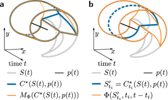
Figure 1: Two sequences that converge to the maximal star-convex material structure $Z(t)$ (a) One iteration step and the final result of sequence (1) which converges fast but is computationally costly. (b) One iteration step of sequence (2) which converges slower but is computationally feasible.

However, the maximal material structures $M_{\Phi}(S^{\prime}(t))$ inside a non-material structure $S^{\prime}(t)$ is quite difficult to find. In principle, many trajectories that start inside $S^{\prime}(t)$ have to be computed to decide which parts leave the structure under advection. For this reason, evaluation of the sequence (1) is computationally unpractical. In contrast, maximal star-convex structures can easily be computed by removing non-star-convex sub-volumes for each time $t\in[0,\tau]$ independently. This is why we propose to never leave the space of material structures in the first place by only enforcing star-convexity for single time points (see Fig. 1).

First, we start with an initial material structure $S(t)$ defined by its volume $S_{t_{1}}=S(t_{1})$ at time $t=t_{1}$. We compute the maximal star-convex volume $S^{1}_{t_{1}}=C^{\star}_{t_{1}}(S(t),p(t))$ by removing everything that is not star-convex at time $t=t_{1}$. This volume defines a new structure $S^{1}(t)$ which is material for all $t\in[0,\tau]$ and star-convex at $t=t_{1}$. Now, we transport this volume using $\Phi$ and see if it remains star-convex. If it does for all $t\in[0,\tau]$, we found our maximal star-convex material structure. If not, we define a new structure $S^{2}(t)$ by again reducing the volume of $S^{1}(t)$ at some time $t=t_{2}$ to its maximal star-convex volume and try again. This way, we define the sequence of structures

$$\begin{split}S^{i}(t)&=\Phi(S^{i}_{t_{i}},t_{i},t-t_{i})\quad\textrm{with}\\ S^{i+1}_{t_{i+1}}&=C^{\star}_{t_{i+1}}(S^{i}(t),p(t))\;.\end{split}$$ (2)

This sequence has the same limit as (1) but is computationally less demanding.

We have seen that the concept of maximal material and maximal star-convex structures leads to an iterative principle for the construction of maximal star-convex material structures $Z(t)$. The only needed parameters are the time interval $[0,\tau]$ and the maximal and minimal estimates $S(t)$ and $p(t)$ represented by there values at $t=0$. All that remains is to specify an explicit algorithm for the sequence (2) that generates the limiting structure $Z(t)$.

Computationally, it is useful to describe a volume $S_{t}$ by its boundary $\hat{S}_{t}$, a so-called material line. These boundaries $\hat{S}_{t}$ will be represented as polygons which can be efficiently transported using the flow $\Phi$ although their number of vertices has to be adjusted regularly to ensure correct approximation of the enclosed volumes. In addition, we introduce the number of time steps $N$, the maximal number of computational cycles $M$, the convergence tolerance $\epsilon$, the maximal vertex distance $\delta$, and the minimal volume $A$. However, these parameters only control the numerical stability and the quality of the results and do not impact the algorithm in any other way.

This finally concludes in the MSCS-search (see Fig. 2):

We start with the time interval $[0,\tau]$, an initial material line $\hat{S}^{1}_{0}$ and an initial position $p_{0}\in\mathbb{R}^{2}$ as maximal and minimal estimates for the structure $Z(t)$ at time $t=0$. We separate the interval in $N$ chunks of length $\Delta\tau$. Then, we successively transport $\hat{S}_{t}^{i}$ and $p_{t}$ into the future, reduce $\hat{S}_{t}^{i}$ to its maximal star-convex volume and fill the boundaries with vertices according to the maximal distance between successive vertices $\delta$. We do this until we reach the end of the interval $t=\tau$ and continue by integrating backwards in time until we complete a full cycle.

If after several such cycles, the material line at some reference time point $t_{\textrm{ref}}$ converges, i.e. if $\frac{\mu(S_{t_{\textrm{ref}}}^{\textrm{ref}})-\mu(S_{t_{\textrm{ref}}}^{i})}{\mu(S_{t_{\textrm{ref}}}^{\textrm{ref}})}<\epsilon$, we found our solution $Z(t)$. Otherwise, if the area becomes too small $\mu(S_{t_{\textrm{ref}}}^{i})<A$ only the trivial solution $Z(t)=p(t)$ remains. If more than $M$ cycles are needed, the structure converges too slowly.

The initial material line $\hat{S}_{0}^{1}$ should be chosen generously and as smooth as possible in order to avoid numerical complications. The initial position $p_{0}$ can be well estimated using simple proxies (see Results).

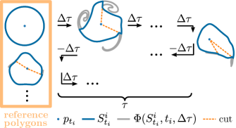
Figure 2: Cutting filaments reveals coherent structures (color online) Starting with an initial polygon $S^{1}_{t_{1}}$ as maximal estimate and a point $p_{t_{1}}$ as a minimal estimate of the star-convex material structure (top left), we successively integrate the material line by $\Delta\tau$ until the end of the desired time-interval $\tau$ is reached (top right). Then we continue by integrating backwards. After each integration we enforce star-convexity of the image $\Phi(S_{t_{i}}^{i},t_{i},t_{i+1}-t_{i})$ with respect to $p_{t_{i+1}}$ and generate a new material line $S_{t_{i+1}}^{i+1}$. If changes between polygons at a reference times point fall below a critical values we stop the integration.

In order to display the potential of our approach, we use the MSCS-search to identify coherent structures in artificial and empirical velocity fields. Moreover, we demonstrate that by changing the observation horizon $\tau$ it is possible to investigate when which parts of the structure are detached or entrained as filaments.

First, we apply our method to flow fields generated by the two-dimensional Euler equation on a square domain with periodic boundary conditions. The two dimensional inviscid flow is initialized with a central large and strong vortex that is surrounded by three smaller and weaker eddies of opposite sense of rotation (see Fig. 3a).

Figure 3: Convex structures for different integration times $\tau$ (color online) (a) Model initialized with large central vortex and three surrounding vortices of different strength. Stream function in the background, dashed lines indicate zero level of Okubo-Weiss criterion. We analyzed three vortices marked by blue crosses which denote the minimal estimates. The blue rectangle denotes the maximal estimate for each structure. (b) Results of analysis for different integration times $\tau$. Medium and larger integration times converge to similar structures of reasonable proportions. Results of the upper left vortex indicate disintegration of any convex structure for larger integration times. (c) Initial positions ($t=0$, left) and final positions ($t=8.4$, right) of test tracers started within the boundaries of the central (blue) and lower (orange) structure for different integration times (light: $\tau=3.6$, dark: $\tau=8.4$). While the boundaries for medium integration times generate filaments, larger integration times result in robust structures.

We want to determine the coherent cores of three eddies: the central strong eddy, the smaller eddy in the upper-left corner and the smaller eddy at the bottom. For this reason, we compute the Okubo-Weiss criterion $Q$ Okubo (1971); Weiss (1991) for the initial velocity field and choose positions $p_{\textrm{ctr},1}$, $p_{\textrm{ul},1}$, $p_{\textrm{bot},1}$ in the vicinity of the corresponding minima. The Okubo-Weiss criterion compares stretching and shear flow with rotation and is an established but Eulerian proxy for vortex positions. The positions $p_{\textrm{ctr},1}$, $p_{\textrm{ul},1}$, $p_{\textrm{bot},1}$ serve as individual minimal estimates for each eddy. For all three eddies, we choose the complete domain as the maximal estimate $\hat{S}_{0}^{1}$ (see Fig. 3a).

We use the MSCS-search for different observation horizons $\tau$ to compute estimates for the largest star-convex material structure $Z(t)$ in each eddy (see Fig. 3b).

The results show that the material lines for small integration times $\tau$ are quite unlikely to correspond to the boundaries of coherent structures. This was to be expected, since the results returned by the MSCS-search are inevitably connected to the predefined time window. In the extreme case of $\tau\rightarrow 0$ the algorithm would simply produce the star-convex initial boundary $\hat{S}_{0}^{1}$.

For larger integration times however, the structures become smaller and smaller and generate a hierarchy of nested sets. Again, this is an expected phenomenon since larger time windows will only generate smaller structures.

The difference between material lines for different integration times corresponds to filaments that are shed from the eddy core in the time between the ends of time windows. Thus, we are able to study the shrinkage of the coherently transported volume. Of course, inverting the time direction would enable the investigation of filament entrainment.

Starting from the eddy in the upper left corner the area enclosed by the star-convex material becomes too small already after intermediate integration times $\tau$. Hence, we conclude that no coherent structure exists for longer time intervals that include the tracer $p_{\textrm{UL},1}$ released at $t=0$.

The inferred material lines of the large central eddy almost appear to converge for longer integration times. This indicates a persistent coherent structure.

In order to test the coherence of the inferred volumes, we release test tracers within the boundaries of the central and the lower vortex at $t=0$ and compute their trajectories until the end of the largest time window $t=8.4$ (see Fig. 3c). We notice that tracer clouds within the boundaries of the star-convex material line inferred for $\tau=3.6$ generate filaments at $t=8.4$ while tracers within the boundaries of the material for $\tau=8.4$ do not, just like our approach predicts. However, it is intriguing that the generated filaments are rather small and remain in the vicinity of the more coherent structure. Thus, even if a volume generates filaments under advection and is thus rejected by our approach, it might still appear to be coherent if these filaments are not resolved.

In addition, we apply the MSCS-search to an open dataset of surface velocities in the North Pacific with spatial and temporal resolution of $0.25\degree$ and $1$ day respectively Risien and Strub (2016) (see Fig. 4). The initial maximal and minimal structures are again chosen on the basis of the Okubo-Weiss criterion (see Fig. 4a) and yield reasonable results for $\tau=12$ and $24$ weeks (see Fig. 4b). The integration of particles reveals that both structures do not generate filaments for $t=12$ weeks and do not even disperse significantly for $t=24$ weeks while the surrounding material generates filaments and mixes with the ambient water (see Fig. 4c/d). During transport, the water mass undergoes considerable contraction.

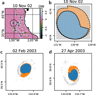
Figure 4: Star convex material structure in the North Pacific (color online) (a) Okubo-Weiss criterion, time and position of initial structures. (b) Results of MSCS-search for $\tau=12$ weeks (orange) and $\tau=24$ weeks (blue) at $t=0$ (c) at $t=12$ weeks and (d) at $t=24$ weeks. Gray tracers indicate mixing with ambient water, most of which leave the displayed domain.

Numerics. The Euler equation is solved using a spectral ansatz with $11$ Fourier components. We realize its integration and the integration of particles using a standard adaptive RK45 scheme. We choose the time step of $\Delta t=0.1$, the maximal vertex distance of $\delta=0.01$ and the minimal polygon area of $A=0.2\cdot 10^{-3}$. To facilitate the search for larger integration times, we initialize their initial maximal estimates $\hat{S}_{0}^{1}$ as the smallest circular polygon with the minimal estimate $p_{0}$ as its center that still contains the results of smaller integration times.

For the oceanic velocity field, the particle integration was realized using linear interpolation in time and space, a standard RK45 approach and a maximal time step of $0.25$ days.

We argued that convexity is an intuitive condition for coherent structures that many established methods could agree on. On this basis, we have used the concept of star-convexity to derive an iterative principle for the estimation of specific volumes that remain star-convex under advection with a flow $\Phi$.

Our MSCS-search algorithm, exploiting this principle, requires little prior knowledge or parameter tuning. It yields convincing results as we demonstrated for both artificial and empirical time dependent velocity fields.

The fixed time window $[0,\tau]$ required by our approach enables us to detect finite-time coherent structures and to study eddy decay and filament entrainment in detail. Additionally, the approach is objective in the sense of Beron-Vera et al. (2013) and able to treat divergent velocity fields as they are typical for surface velocities. Moreover, it does not depend on auxiliary parameters that must be tweaked or tuned to generate desired results. Instead, all additional parameters only control the algorithm’s numerical stability. Their ideal values are known and their impact is self-explanatory. In conclusion, this approach seems well applicable to real oceanic velocity fields.

Future extensions could for instance include avoidance of unnecessary repeated particle integrations and the enabling of parallel computation.

References

- Arístegui et al. (1997) J. Arístegui, P. Tett, A. Hernández-Guerra, G. Basterretxea, M. F. Montero, K. Wild, P. Sangrá, S. Hernández-León, M. Cantón, J. A. García-Braun, M. Pacheco, and E. D. Barton, Deep-Sea Research Part I: Oceanographic Research Papers 44, 71 (1997).
- Martin (2003) A. Martin, Progress in Oceanography 57, 125 (2003).
- Beal et al. (2011) L. M. Beal, W. P. M. De Ruijter, A. Biastoch, R. Zahn, M. Cronin, J. Hermes, J. Lutjeharms, G. Quartly, T. Tozuka, S. Baker-Yeboah, T. Bornman, P. Cipollini, H. Dijkstra, I. Hall, W. Park, F. Peeters, P. Penven, H. Ridderinkhof, and J. Zinke, Nature 472, 429 (2011).
- Dong et al. (2014) C. Dong, J. C. McWilliams, Y. Liu, and D. Chen, Nature Communications 5, 3294 (2014).
- Karstensen et al. (2015) J. Karstensen, B. Fiedler, F. Schütte, P. Brandt, A. Körtzinger, G. Fischer, R. Zantopp, J. Hahn, M. Visbeck, and D. Wallace, Biogeosciences 12, 2597 (2015).
- McGillicuddy Jr. (2016) D. J. McGillicuddy Jr., Annual Review of Marine Science 8, 125 (2016).
- Prants et al. (2014) S. Prants, M. Budyansky, and M. Uleysky, Deep Sea Research Part I: Oceanographic Research Papers 90, 27 (2014), 1208.0647 .
- D’Ovidio et al. (2010) F. D’Ovidio, S. De Monte, S. Alvain, Y. Dandonneau, and M. Levy, Proceedings of the National Academy of Sciences 107, 18366 (2010).
- D’Ovidio et al. (2013) F. D’Ovidio, S. De Monte, A. D. Penna, C. Cotté, and C. Guinet, Journal of Physics A: Mathematical and Theoretical 46, 254023 (2013).
- Richardson (2007) P. L. Richardson, Deep Sea Research Part I: Oceanographic Research Papers 54, 1361 (2007).
- Beron-Vera et al. (2013) F. J. Beron-Vera, Y. Wang, M. J. Olascoaga, G. J. Goni, and G. Haller, Journal of Physical Oceanography 43, 1426 (2013).
- Froyland et al. (2015) G. Froyland, C. Horenkamp, V. Rossi, and E. van Sebille, Chaos: An Interdisciplinary Journal of Nonlinear Science 25, 083119 (2015).
- Bracco et al. (2000) A. Bracco, A. Provenzale, and I. Scheuring, Proceedings of the Royal Society of London. Series B: Biological Sciences 267, 1795 (2000).
- Sandulescu et al. (2007) M. Sandulescu, C. López, E. Hernández-García, and U. Feudel, Nonlinear Processes in Geophysics 14, 443 (2007), 0802.3973 .
- Gaube et al. (2014) P. Gaube, D. J. McGillicuddy Jr., D. B. Chelton, M. J. Behrenfeld, and P. G. Strutton, Journal of Geophysical Research: Oceans 119, 8195 (2014).
- Okubo (1971) A. Okubo, Deep-Sea Research and Oceanographic Abstracts 18, 789 (1971).
- Weiss (1991) J. Weiss, Physica D: Nonlinear Phenomena 48, 273 (1991).
- Isern-Fontanet et al. (2003) J. Isern-Fontanet, E. García-Ladona, and J. Font, Journal of Atmospheric and Oceanic Technology 20, 772 (2003).
- Chaigneau et al. (2008) A. Chaigneau, A. Gizolme, and C. Grados, Progress in Oceanography 79, 106 (2008).
- Itoh and Yasuda (2010) S. Itoh and I. Yasuda, Journal of Physical Oceanography 40, 1018 (2010).
- Chelton et al. (2011) D. B. Chelton, M. G. Schlax, and R. M. Samelson, Progress in Oceanography 91, 167 (2011).
- Nencioli et al. (2010) F. Nencioli, C. Dong, T. Dickey, L. Washburn, and J. C. Mcwilliams, Journal of Atmospheric and Oceanic Technology 27, 564 (2010).
- Mendoza and Mancho (2010) C. Mendoza and A. M. Mancho, Physical Review Letters 105, 1 (2010).
- Mancho et al. (2013) A. M. Mancho, S. Wiggins, J. Curbelo, and C. Mendoza, Communications in Nonlinear Science and Numerical Simulation 18, 3530 (2013).
- Rypina et al. (2011) I. I. Rypina, S. E. Scott, L. J. Pratt, and M. G. Brown, Nonlinear Processes in Geophysics 18, 977 (2011).
- Froyland and Padberg-Gehle (2015) G. Froyland and K. Padberg-Gehle, Chaos: An Interdisciplinary Journal of Nonlinear Science 25, 087406 (2015).
- Hadjighasem et al. (2016) A. Hadjighasem, D. Karrasch, H. Teramoto, and G. Haller, Physical Review E 93, 1 (2016), 1506.02258 .
- Vortmeyer-Kley et al. (2016) R. Vortmeyer-Kley, U. Gräwe, and U. Feudel, Nonlinear Processes in Geophysics 23, 159 (2016).
- Froyland (2013) G. Froyland, Physica D: Nonlinear Phenomena 250, 1 (2013).
- Ma and Bollt (2013) T. Ma and E. M. Bollt, International Journal of Bifurcation and Chaos 23, 1330026 (2013).
- Froyland and Padberg-Gehle (2014) G. Froyland and K. Padberg-Gehle, in Springer Proceedings in Mathematics and Statistics, Vol. 70 (2014) pp. 171–216.
- Lünsmann et al. (2018) B. J. Lünsmann, R. Vortmeyer-kley, and H. Kantz, (under review) , 5 (2018), arXiv:1903.05086v1 .
- Boffetta et al. (2001) G. Boffetta, G. Lacorata, G. Redaelli, and A. Vulpiani, Physica D: Nonlinear Phenomena 159, 58 (2001), 0102022 [nlin] .
- Shadden et al. (2005) S. C. Shadden, F. Lekien, and J. E. Marsden, Physica D: Nonlinear Phenomena 212, 271 (2005).
- Haller (2015) G. Haller, Annual Review of Fluid Mechanics 47, 137 (2015), 1407.4072 .
- Haller et al. (2016) G. Haller, A. Hadjighasem, M. Farazmand, and F. Huhn, Journal of Fluid Mechanics 795, 136 (2016), 1506.04061 .
- Hadjighasem et al. (2017) A. Hadjighasem, M. Farazmand, D. Blazevski, G. Froyland, and G. Haller, Chaos: An Interdisciplinary Journal of Nonlinear Science 27, 053104 (2017), 1704.05716 .
- Beron-Vera et al. (2018) F. J. Beron-Vera, M. J. Olascoaga, Y. Wang, J. Triñanes, and P. Pérez-Brunius, Scientific Reports 8, 1 (2018), 1704.06186 .
- Risien and Strub (2016) C. M. Risien and P. T. Strub, Sci. Data 3, 160013 (2016).