High-order accurate entropy stable finite difference schemes for one- and two-dimensional special relativistic hydrodynamics

Abstract

This paper develops the high-order accurate entropy stable finite difference schemes for one- and two-dimensional special relativistic hydrodynamic equations. The schemes are built on the entropy conservative flux and the weighted essentially non-oscillatory (WENO) technique as well as explicit Runge-Kutta time discretization. The key is to technically construct the affordable entropy conservative flux of the semi-discrete second-order accurate entropy conservative schemes satisfying the semi-discrete entropy equality for the found convex entropy pair. As soon as the entropy conservative flux is derived, the dissipation term can be added to give the semi-discrete entropy stable schemes satisfying the semi-discrete entropy inequality with the given convex entropy function. The WENO reconstruction for the scaled entropy variables and the high-order explicit Runge-Kutta time discretization are implemented to obtain the fully-discrete high-order entropy stable schemes. Several numerical tests are conducted to validate the accuracy and the ability to capture discontinuities of our entropy stable schemes.

Keywords: Entropy conservative scheme, entropy stable scheme, high order accuracy, finite difference scheme, special relativistic hydrodynamics.

1 Introduction

This paper is concerned with the high-order accurate numerical schemes for the one- and two-dimensional special relativistic hydrodynamic (RHD) equations, which in the laboratory frame, can be cast in the divergence form

$$\dfrac{\partial{\bm{U}}}{\partial{t}}+\sum_{\ell=1}^{d}\dfrac{\partial{\bm{F}_{\ell}(\bm{U})}}{\partial{x_{\ell}}}=0,$$ (1)

where $\bm{U}$ and $\bm{F}_{\ell}$ are respectively the conservative vector and the flux vector in the $x_{\ell}$-direction and defined by

$$\begin{aligned} &\bm{U}=(D,m_{1},\cdots,m_{d},E)^{\mathrm{T}},\\ &\bm{F}_{\ell}=(Du_{\ell},m_{1}u_{\ell}+p\delta_{1,\ell},\cdots,m_{d}u_{\ell}+p\delta_{d,\ell},m_{\ell})^{\mathrm{T}},\quad\ell=1,\ldots,d,\end{aligned}$$ (2)

with the mass density $D=\rho W$, the momentum density $\bm{m}=(m_{1},\cdots,m_{d})^{\mathrm{T}}=DhW\bm{u}$, and the energy density $E=DhW-p$. Here, $d=1$ or 2, $\rho,p$ and $\bm{u}=(u_{1},\cdots,u_{d})^{\mathrm{T}}$ denote the rest-mass density, the kinetic pressure, and the fluid velocity, respectively. Moreover, $W=1/\sqrt{1-(u_{1}^{2}+\cdots+u_{d}^{2})}$ is the Lorentz factor and $h$ is the specific enthalpy defined by $h=1+e+p/\rho$ with units in which the speed of light is equal to one, and the specific internal energy $e$. The system (1)-(2) should be closed by using the equation of state (EOS). This paper will only consider the ideal-fluid EOS

$$p=(\Gamma-1)\rho e,$$

with the adiabatic index $\Gamma\in(1,2]$. Because there is no explicit expression for the primitive variables $(\rho,\bm{u}^{\mathrm{T}},p)$ and the flux $\bm{F}_{\ell}$ in terms of $\bm{U}$, in order to recover the values of the primitive variables and the flux from the given $\bm{U}$, a nonlinear algebraic equation such as

$$E+p=DW+\dfrac{\Gamma}{\Gamma-1}pW^{2},$$

has to be numerically solved to obtain the pressure $p$, and then the rest-mass density $\rho$, the specific enthalpy $h$, and the velocity $\bm{u}$ can be orderly calculated by

$$\rho=\dfrac{D}{W},\quad h=1+\dfrac{\Gamma p}{(\Gamma-1)\rho},\quad\bm{u}=\dfrac{\bm{m}}{Dh}.$$

The relativistic description for the dynamics of the fluid (gas) at nearly speed of light should be considered when we investigate the astrophysical phenomena from stellar to galactic scales, e.g. coalescing neutron stars, core collapse supernovae, active galactic nuclei, superluminal jets, formation of black holes, and gamma-ray bursts etc. Due to the relativistic effect, the nonlinearity of the system (1)-(2) becomes much stronger than the non-relativistic case so that its analytic treatment is extremely difficult and challenging. Numerical simulation is a primary way to help our understanding the physical mechanisms in the RHD. It can be traced back to the artificial viscosity method for the RHD equations in the Lagrangian coordinates [28, 29] and in the Eulerian coordinates [39]. After those, the modern shock-captured methods for the RHD equations would not be noticed until later. Here listed are some works: the Harten-Lax-van Leer method [36], the two-shock solvers [1, 7], the Roe solver [9], the essentially non-oscillatory (ENO) and the weighted ENO (WENO) methods [8, 51], the piecewise parabolic methods [25, 31], the adaptive mesh refinement method [52], the Runge-Kutta discontinuous Galerkin methods with WENO limiter [53], the direct Eulerian generalized Riemann problem schemes [49, 50, 48, 43], the adaptive moving mesh methods [17, 18], and so on. The readers are referred to the early review articles [26, 14, 27] and references therein. Recently, the properties of the admissible state set and the physical-constraints-preserving (PCP) numerical schemes were well studied for the RHD, see [45, 47, 40] and [34], and for the special relativistic magnetohydrodynamics [44, 46]. The PCP schemes satisfy that both the rest-mass density and the kinetic pressure are positive and the magnitude of the fluid velocity is less than the speed of light. Motivated by [44, 46], the positivity-preserving schemes for the non-relativistic ideal magnetohydrodynamics were successfully studied in [41, 42].

It is well known that the weak solution of the quasi-linear hyperbolic conservation laws might not be unique so that the entropy conditions are needed to single out the physical relevant solution among all weak solutions.

Definition 1 (Entropy function)

A strictly convex function $\eta(\bm{U})$ is called an entropy function for the system (1)-(2) if there are associated entropy fluxes $q_{\ell}(\bm{U})$ such that

$$q_{\ell}^{\prime}(\bm{U})=\bm{V}^{\mathrm{T}}\bm{F}_{\ell}^{\prime}(\bm{U}),\quad\ell=1,\cdots,d,$$ (3)

where $\bm{V}=\eta^{\prime}(\bm{U})^{\mathrm{T}}$ is called the entropy variables, and $(\eta,q_{\ell})$ is an entropy pair.

For the smooth solutions of (1)-(2), multiplying (1) by $\bm{V}^{\mathrm{T}}$ gives the entropy identity

$$\eta(\bm{U})_{t}+\sum_{l=1}^{d}q_{l}(\bm{U})_{x_{l}}=0.$$

However, if the solutions contain discontinuity, then the above identity does not hold.

Definition 2 (Entropy solution)

A weak solution $\bm{U}$ of (1) is called an entropy solution if for all entropy functions $\eta$, the inequality

$$\eta(\bm{U})_{t}+\sum_{l=1}^{d}q_{l}(\bm{U})_{x_{l}}\leq 0,$$ (4)

holds in the sense of distributions.

Formally, integrating (4) in space and imposing a periodic or no-inflow boundary conditions gets the inequality $\dfrac{\mathrm{d}}{\mathrm{d}t}\int_{\mathbb{R}}\eta(\bm{U})\mathrm{d}\bm{x}\leq 0$, which can be converted into an a priori estimate on the solution of (1) in a suitable $L^{p}$ space if $\eta$ is convex [11, 6]. The entropy conditions are of great importance in the well-posedness of hyperbolic conservation laws, thus it is reasonable to seek the entropy stable schemes of (1), satisfying a discrete or semi-discrete version of the entropy inequality (4). For the smooth solutions of the special RHD equations (1)-(2), the thermodynamic entropy

$$S=\ln(p)-\Gamma\ln(\rho),$$

satisfies

$$\dfrac{\partial{(\rho WS)}}{\partial{t}}+\sum_{\ell=1}^{d}\dfrac{\partial{(\rho u_{\ell}WS)}}{\partial{x_{\ell}}}=0,$$

thus an entropy pair of (1)-(2) can be defined by

$$\eta(\bm{U})=\dfrac{-\rho WS}{\Gamma-1},\quad q_{\ell}(\bm{U})=\dfrac{-\rho u_{\ell}WS}{\Gamma-1},\quad\ell=1,\cdots,d,$$

and corresponding entropy variables $\bm{V}=\eta^{\prime}(\bm{U})^{\mathrm{T}}$ can be explicitly given by

$$\bm{V}=\left(\dfrac{\Gamma-S}{\Gamma-1}+\dfrac{\rho}{p},\dfrac{\rho W\bm{u}^{\mathrm{T}}}{p},-\dfrac{\rho W}{p}\right)^{\mathrm{T}},$$

which gives the “potential” $\psi_{\ell}:=\bm{V}^{T}\bm{F}_{\ell}(\bm{U})-q_{\ell}(\bm{U})=\rho Wu_{\ell}$, $\ell=1,\cdots,d$. It can be verified that, for $d=1,2$, the matrices $\dfrac{\partial{\bm{U}}}{\partial{\bm{V}}}$ and $\dfrac{\partial{\bm{F}_{\ell}}}{\partial{\bm{U}}}\dfrac{\partial{\bm{U}}}{\partial{\bm{V}}}$ are symmetric and $\dfrac{\partial{\bm{U}}}{\partial{\bm{V}}}$ is positive definite so that (1)-(2) can be symmetrized with the above entropy pair. Such symmetrization of the RHD equations (1)-(2) will be useful in deriving a set of particular scaled eigenvectors used for designing the dissipation term of the entropy stable schemes in Section 2.2.

For the scalar conservation laws, the conservative monotone schemes were shown that they were nonlinearly stable and satisfied the discrete entropy conditions so that they could converge to the entropy solution [16, 5]. A class of so-called E-schemes satisfying the entropy condition for any convex entropy were studied in [32, 33]. Those schemes are only first-order accurate. Due to the fact that it is basically impossible to show that the high-order schemes of the scalar conservation laws and the schemes for the system of hyperbolic conservation laws satisfy the entropy inequality for any convex entropy pair, the researcher tries to study the high-order accurate entropy stable schemes, which satisfy the entropy inequality for a given entropy pair. The second-order entropy conservative schemes (satisfying the discrete entropy identity) were built in [37, 38], and their higher-order extension was introduced in [22]. It is known that an entropy conservative scheme may become oscillatory near the shock wave, thus the additional dissipation terms has to be added to the entropy conservative schemes to obtain the entropy stable schemes. Combining the entropy conservative flux of the entropy conservative schemes with the “sign” property of the ENO reconstructions, the arbitrary high-order entropy stable schemes were constructed by using high-order dissipation terms [11]. Some entropy stable schemes based on the DG framework were studied, such as [2, 19] in the space-time DG formulation, the entropy stable nodal DG schemes using suitable quadrature rules [4], and its extension to magnetohydrodynamics equations [24]. The entropy stable schemes based on summation-by-parts (SBP) operators were developed for the Navier-Stokes equations [10]. The existing works do not address the entropy stable schemes for the special or general RHD equations.

The paper aims at constructing the high-order accurate entropy stable schemes for one- and two-dimensional special RHD equations (1)-(2). The key is to technically construct the affordable entropy conservative flux of the semi-discrete second-order accurate entropy conservative schemes satisfying the semi-discrete entropy equality for the found convex entropy pair. The paper is organized as follows. Section 2 introduces the entropy conservative fluxes, entropy conservative schemes, and entropy stable schemes for the one-dimensional special RHD equations. Section 3 introduces our schemes for the two-dimensional special RHD equations. Several one- and two-dimensional numerical tests are conducted in Section 4 to validate the effectiveness of our schemes. Some conclusions are summarized in Section 5.

2 One-dimensional schemes

This section considers the one-dimensional special RHD equations, i.e., (1)-(2) with $d=1$. For the sake of convenience, the notations $\bm{F}_{1},u_{1},m_{1}$ and $x_{1}$ are replaced with $\bm{F},u,m$ and $x$, respectively, so that the flux, the entropy pair and the potential become $\bm{F}=(Du,mu+p,m)^{\mathrm{T}}$, $\eta=\dfrac{-\rho WS}{\Gamma-1}$, $q=\dfrac{-\rho uWS}{\Gamma-1}$, and $\psi=\rho uW$, respectively.

Let us consider a uniform mesh $x_{1}<x_{2}<\cdots<x_{N}$ with the step size $\Delta x=x_{i}-x_{i-1},~{}i=2,\cdots,N$ and the semi-discrete conservative finite difference scheme

$$\dfrac{\mathrm{d}}{\mathrm{d}t}\bm{U}_{i}(t)=-\dfrac{1}{\Delta x}\left(\hat{\bm{F}}_{{i+\frac{1}{2}}}(t)-\hat{\bm{F}}_{{i-\frac{1}{2}}}(t)\right),$$ (5)

where $\bm{U}_{i}(t)$ approximates the point value of $\bm{U}(x_{i},t)$ and $\hat{\bm{F}}_{{i+\frac{1}{2}}}$ is the numerical flux approximating $\bm{F}$ at $x_{{i+\frac{1}{2}}}=x_{i}+{\Delta x}/{2}$.

2.1 Entropy conservative fluxes

Definition 3 (Entropy conservative scheme)

The scheme (5) is called entropy conservative scheme if its solution satisfies a semi-discrete entropy equality

$$\dfrac{\mathrm{d}}{\mathrm{d}t}\eta(\bm{U}_{i}(t))=-\dfrac{1}{\Delta x}\left(\tilde{q}_{{i+\frac{1}{2}}}(t)-\tilde{q}_{{i-\frac{1}{2}}}(t)\right),$$ (6)

for some numerical entropy flux $\tilde{q}_{{i+\frac{1}{2}}}$ consistent with $q$.

Theorem 1 (Tadmor[37])

If a consistent numerical flux $\tilde{\bm{F}}_{{i+\frac{1}{2}}}$ satisfies

$$\llbracket\bm{V}\rrbracket^{\mathrm{T}}_{{i+\frac{1}{2}}}\tilde{\bm{F}}_{{i+\frac{1}{2}}}=\llbracket\psi\rrbracket_{{i+\frac{1}{2}}},$$ (7)

with $\llbracket a\rrbracket_{{i+\frac{1}{2}}}:=a_{i+1}-a_{i}$ and $\{\!\!\{a\}\!\!\}_{{i+\frac{1}{2}}}:=\dfrac{1}{2}(a_{i}+a_{i+1})$, then the scheme (5) with $\tilde{\bm{F}}_{{i+\frac{1}{2}}}$ is second-order accurate and entropy conservative. The corresponding numerical entropy flux is $\tilde{q}_{{i+\frac{1}{2}}}=\{\!\!\{\bm{V}\}\!\!\}^{\mathrm{T}}_{{i+\frac{1}{2}}}\tilde{\bm{F}}_{{i+\frac{1}{2}}}-\{\!\!\{\psi\}\!\!\}_{{i+\frac{1}{2}}}$.

For the scalar equation, solving (7) can uniquely give $\tilde{\bm{F}}_{{i+\frac{1}{2}}}$, but it is not clear for a general system. In [37], a solution of (7) was constructed by the path integral in the phase space

$$\tilde{\bm{F}}_{{i+\frac{1}{2}}}=\int_{0}^{1}\bm{F}(\bm{V}_{i}+\xi(\bm{V}_{i+1}-\bm{V}_{i}))\mathrm{d}\xi,$$ (8)

which might be very hard to calculate except in some special cases[12]. An explicit solution of (7) was given in [38], but it was both expensive and numerically unstable. Some explicit algebraic solutions of (7) were constructed in the literature for the specific systems, such as the linear symmetric system, the shallow water equations [12], the Euler equations [20]. Herein, we construct the affordable entropy conservative flux for the one-dimensional special RHD equations using the strategy introduced in [35]. The key is to use the identity

$$\llbracket ab\rrbracket=\{\!\!\{a\}\!\!\}\llbracket b\rrbracket+\{\!\!\{b\}\!\!\}\llbracket a\rrbracket,$$

where $\llbracket a\rrbracket$ and $\{\!\!\{a\}\!\!\}$ denote the jump and mean of $a$, respectively, and rewrite the jumps of the entropy variables ${\bm{V}}$ and the potential ${\psi}$ as some linear combinations of the jump of a specially chosen parameter vector. To be specific, we first deal with the Lorentz factor and omit the subscript $i$ for simplicity. Because

$$\dfrac{1}{\sqrt{1-u_{R}^{2}}}-\dfrac{1}{\sqrt{1-u_{L}^{2}}}=\dfrac{(u_{L}+u_{R})(u_{R}-u_{L})}{\sqrt{1-u_{L}^{2}}\sqrt{1-u_{R}^{2}}(\sqrt{1-u_{L}^{2}}+\sqrt{1-u_{R}^{2}})},$$

where the subscripts $L$ and $R$ denote the left and right values of the variables used to calculate the entropy conservative flux, one can define the “Lorentz mean” by

$$\llbracket W\rrbracket=\{\!\!\{u\}\!\!\}^{\text{Lor}}\llbracket u\rrbracket,$$

where

$$\{\!\!\{u\}\!\!\}^{\text{Lor}}=\dfrac{u_{L}+u_{R}}{\sqrt{1-u_{L}^{2}}\sqrt{1-u_{R}^{2}}(\sqrt{1-u_{L}^{2}}+\sqrt{1-u_{R}^{2}})}.$$ (9)

If choosing the parameter vector

$$\bm{z}=(z_{1},z_{2},z_{3})^{\mathrm{T}}=(\rho,\rho/p,u)^{\mathrm{T}},$$

then

$$\left\{\begin{aligned} &\llbracket\bm{V}_{1}\rrbracket=\dfrac{\llbracket z_{1}\rrbracket}{\{\!\!\{z_{1}\}\!\!\}^{\text{ln}}}+\dfrac{1}{\Gamma-1}\dfrac{\llbracket z_{2}\rrbracket}{\{\!\!\{z_{2}\}\!\!\}^{\text{ln}}}+\llbracket z_{2}\rrbracket,\\ &\llbracket\bm{V}_{2}\rrbracket=\{\!\!\{uW\}\!\!\}\llbracket z_{2}\rrbracket+\{\!\!\{z_{2}\}\!\!\}\{\!\!\{W\}\!\!\}\llbracket z_{3}\rrbracket+{\{\!\!\{z_{2}\}\!\!\}\{\!\!\{z_{3}\}\!\!\}{\{\!\!\{z_{3}\}\!\!\}^{\text{Lor}}}\llbracket z_{3}\rrbracket},\\ &\llbracket\bm{V}_{3}\rrbracket=-\{\!\!\{W\}\!\!\}\llbracket z_{2}\rrbracket-\{\!\!\{z_{2}\}\!\!\}{\{\!\!\{z_{3}\}\!\!\}^{\text{Lor}}}{\llbracket z_{3}\rrbracket},\\ &\llbracket\psi\rrbracket=\{\!\!\{uW\}\!\!\}\llbracket z_{1}\rrbracket+\{\!\!\{z_{1}\}\!\!\}\{\!\!\{W\}\!\!\}\llbracket z_{3}\rrbracket+\{\!\!\{z_{1}\}\!\!\}\{\!\!\{z_{3}\}\!\!\}{\{\!\!\{z_{3}\}\!\!\}^{\text{Lor}}}{\llbracket z_{3}\rrbracket},\end{aligned}\right.$$ (10)

where $\{\!\!\{a\}\!\!\}^{\text{ln}}={\llbracket a\rrbracket}/{\llbracket\ln{a}\rrbracket}$ is the logarithmic mean introduced in [20], where its stable numerical implementation can be found. If assuming that the entropy conservative flux is $\tilde{\bm{F}}=(\tilde{\bm{F}}_{1},\tilde{\bm{F}}_{2},\tilde{\bm{F}}_{3})^{\mathrm{T}}$, and substituting the equations (10) in (7), then

$$\left\{\begin{aligned} &\dfrac{\tilde{\bm{F}}_{1}}{\{\!\!\{z_{1}\}\!\!\}^{\text{ln}}}=\{\!\!\{uW\}\!\!\},\\ &\dfrac{\tilde{\bm{F}}_{1}}{(\Gamma-1)\{\!\!\{z_{2}\}\!\!\}^{\text{ln}}}+\tilde{\bm{F}}_{1}+\{\!\!\{uW\}\!\!\}{\tilde{\bm{F}}_{2}}-\{\!\!\{W\}\!\!\}\tilde{\bm{F}}_{3}=0,\\ &\tilde{\bm{F}}_{2}\{\!\!\{z_{2}\}\!\!\}(\{\!\!\{W\}\!\!\}+\{\!\!\{z_{3}\}\!\!\}{\{\!\!\{z_{3}\}\!\!\}^{\text{Lor}}})-{{\tilde{\bm{F}}_{3}}\{\!\!\{z_{2}\}\!\!\}}{\{\!\!\{z_{3}\}\!\!\}^{\text{Lor}}}=\{\!\!\{z_{1}\}\!\!\}(\{\!\!\{W\}\!\!\}+{\{\!\!\{z_{3}\}\!\!\}}{\{\!\!\{z_{3}\}\!\!\}^{\text{Lor}}}).\end{aligned}\right.$$

Solving the above equations can obtain the entropy conservative flux for the one-dimensional special RHD equations as follows

$$\left\{\begin{aligned} \tilde{\bm{F}}_{1}=&\{\!\!\{z_{1}\}\!\!\}^{\text{ln}}\{\!\!\{uW\}\!\!\},\\ \tilde{\bm{F}}_{2}=&Q^{-1}\Bigg{[}\left(1+\dfrac{1}{(\Gamma-1)\{\!\!\{z_{2}\}\!\!\}^{\text{ln}}}\right){\{\!\!\{z_{2}\}\!\!\}}{\{\!\!\{z_{3}\}\!\!\}^{\text{Lor}}}\tilde{\bm{F}}_{1}+\{\!\!\{z_{1}\}\!\!\}\{\!\!\{W\}\!\!\}^{2}\\ &+{\{\!\!\{z_{1}\}\!\!\}\{\!\!\{z_{3}\}\!\!\}\{\!\!\{W\}\!\!\}}{\{\!\!\{z_{3}\}\!\!\}^{\text{Lor}}}\Bigg{]},\\ \tilde{\bm{F}}_{3}=&Q^{-1}\Bigg{[}\{\!\!\{z_{1}\}\!\!\}\{\!\!\{W\}\!\!\}\{\!\!\{uW\}\!\!\}+{\{\!\!\{z_{1}\}\!\!\}\{\!\!\{z_{3}\}\!\!\}\{\!\!\{uW\}\!\!\}}{\{\!\!\{z_{3}\}\!\!\}^{\text{Lor}}}\\ &+\left(1+\dfrac{1}{(\Gamma-1)\{\!\!\{z_{2}\}\!\!\}^{\text{ln}}}\right)\tilde{\bm{F}}_{1}\left(\{\!\!\{z_{2}\}\!\!\}\{\!\!\{W\}\!\!\}+{\{\!\!\{z_{2}\}\!\!\}\{\!\!\{z_{3}\}\!\!\}}{\{\!\!\{z_{3}\}\!\!\}^{\text{Lor}}}\right)\Bigg{]},\end{aligned}\right.$$ (11)

where $Q=\{\!\!\{z_{2}\}\!\!\}\{\!\!\{W\}\!\!\}^{2}+{\{\!\!\{z_{2}\}\!\!\}\{\!\!\{z_{3}\}\!\!\}\{\!\!\{W\}\!\!\}}{\{\!\!\{z_{3}\}\!\!\}^{\text{Lor}}}-{\{\!\!\{z_{2}\}\!\!\}\{\!\!\{uW\}\!\!\}}{\{\!\!\{z_{3}\}\!\!\}^{\text{Lor}}}$.

Remark 1

It is worth noting that $Q$ in the above expressions is positive so that our entropy conservative flux is well defined. In fact, if $u_{L}=u_{R}$ and $W_{L}=W_{R}$, then $\{\!\!\{z_{3}\}\!\!\}^{\text{Lor}}=\{\!\!\{u\}\!\!\}^{\text{Lor}}=u_{L}W_{L}^{3}$ due to (9), thus $Q=\{\!\!\{z_{2}\}\!\!\}W_{L}^{2}>0$; otherwise, $\{\!\!\{z_{3}\}\!\!\}^{\text{Lor}}=\{\!\!\{u\}\!\!\}^{\text{Lor}}={\llbracket W\rrbracket}/{\llbracket u\rrbracket}$, thus

$$Q =\{\!\!\{z_{2}\}\!\!\}\left\{\dfrac{(W_{L}+W_{R})^{2}}{4}+\left[\dfrac{u_{L}+u_{R}}{2}\dfrac{W_{L}+W_{R}}{2}-\dfrac{u_{L}W_{L}+u_{R}W_{R}}{2}\right]\dfrac{W_{L}-W_{R}}{u_{L}-u_{R}}\right\}$$

$$=\{\!\!\{z_{2}\}\!\!\}W_{L}W_{R}>0.$$

Remark 2

It is also easy to verify that the entropy conservative flux (11) is consistent with the flux $\bm{F}$. If letting $(\rho_{L},u_{L},p_{L})=(\rho_{R},u_{R},p_{R})=(\rho,u,p)$, then

$$\tilde{\bm{F}}_{1}= \rho{uW},$$

$$\tilde{\bm{F}}_{2}= \dfrac{\left(1+\dfrac{p}{(\Gamma-1)\rho}\right)\dfrac{{\rho^{2}}{u^{2}W^{4}}}{p}+\rho{W}^{2}+{\rho u^{2}W^{4}}}{\rho W^{2}/p}=\rho hW^{2}u^{2}+p,$$

$$\tilde{\bm{F}}_{3}= \dfrac{\rho W^{2}u+\rho W^{4}u^{3}+\left(1+\dfrac{p}{(\Gamma-1)\rho}\right)\dfrac{{\rho^{2}W^{2}u+\rho^{2}W^{4}u^{3}}}{p}}{\rho W^{2}/p}=\rho hW^{2}u.$$

The scheme (5) with the entropy conservative flux (11) is only second-order accurate. However, if using that entropy conservative flux as a building block, then one can obtain an entropy conservative flux of the $2p$th-order ($p\in\mathbb{N}^{+}$) accurate scheme by using the linear combinations of the “second-order accurate” entropy conservative fluxes [22]. Here only presents the specific expressions for the “$6$th-order accurate” entropy conservative flux

$$\tilde{\bm{F}}^{6\mbox{\scriptsize th}}_{{i+\frac{1}{2}}}= \dfrac{3}{2}\tilde{\bm{F}}(\bm{U}_{i},\bm{U}_{i+1})-\dfrac{3}{10}\left(\tilde{\bm{F}}(\bm{U}_{i-1},\bm{U}_{i+1})+\tilde{\bm{F}}(\bm{U}_{i},\bm{U}_{i+2})\right)$$

$$+\dfrac{1}{30}\left(\tilde{\bm{F}}(\bm{U}_{i-2},\bm{U}_{i+1})+\tilde{\bm{F}}(\bm{U}_{i-1},\bm{U}_{i+2})+\tilde{\bm{F}}(\bm{U}_{i},\bm{U}_{i+3})\right).$$ (12)

The readers are referred to [22, 11] for more details on constructing the “high-order accurate” entropy conservative flux.

2.2 Entropy stable fluxes

The entropy of hyperbolic conservation laws is conserved only if the solution is smooth. In other words, the entropy is not conserved if the discontinuity such as the shock wave appears in the solution. It is well-known that an entropy conservative scheme may become oscillatory near the shock wave, thus we expect to construct an entropy stable scheme by adding a dissipation term in the original entropy conservative scheme. This section will first introduce the entropy stable flux and its high-order extension of Tadmor and his collaborators via the ENO reconstruction, and then go to the low dissipative entropy stable flux by using a switch function in the dissipation term [3].

Theorem 2 (Tadmor[37])

If assuming that $\bm{D}_{{i+\frac{1}{2}}}$ is a symmetric positive semi-definite matrix and $\tilde{\bm{F}}_{{i+\frac{1}{2}}}$ is an entropy conservative flux, then the scheme (5) with the following numerical flux

$$\hat{\bm{F}}_{{i+\frac{1}{2}}}=\tilde{\bm{F}}_{{i+\frac{1}{2}}}-\dfrac{1}{2}\bm{D}_{{i+\frac{1}{2}}}\llbracket\bm{V}\rrbracket_{{i+\frac{1}{2}}},$$ (13)

is entropy stable, i.e., satisfying the semi-discrete entropy inequality

$$\dfrac{\mathrm{d}}{\mathrm{d}t}\eta(\bm{U}_{i}(t))+\dfrac{1}{\Delta x}\left(\hat{q}_{{i+\frac{1}{2}}}(t)-\hat{q}_{{i-\frac{1}{2}}}(t)\right)\leq 0,$$

for some numerical entropy flux function $\hat{q}_{{i+\frac{1}{2}}}$ consistent with $q$.

The above theorem holds for any positive semi-definite matrix $\bm{D}_{{i+\frac{1}{2}}}$, which is usually chosen as

$$\bm{D}_{{i+\frac{1}{2}}}=\bm{R}_{{i+\frac{1}{2}}}\lvert\bm{\Lambda}_{{i+\frac{1}{2}}}\rvert\bm{R}_{{i+\frac{1}{2}}}^{\mathrm{T}},$$

where $\bm{R}$ is a scaled matrix of right eigenvectors, whose existence can be ensured by the eigenvector scaling theorem in [30], and satisfies

$$\dfrac{\partial{\bm{F}}}{\partial{\bm{U}}}=\bm{R}\bm{\Lambda}\bm{R}^{-1},\quad\bm{U}_{\bm{V}}=\bm{R}\bm{R}^{\mathrm{T}}.$$

For the one-dimensional special RHD equations, after some algebraic manipulations, the scaled matrix $\bm{R}$ is

$$\begin{bmatrix}1&1&1\\ (u-c_{s})Wh&uW&(u+c_{s})Wh\\ (1-uc_{s})Wh&W&(1+uc_{s})Wh\\ \end{bmatrix}\begin{bmatrix}\frac{\rho W(1-uc_{s})}{2\Gamma}&0&0\\ 0&\frac{(\Gamma-1)\rho W}{\Gamma}&0\\ 0&0&\frac{\rho W(1+uc_{s})}{2\Gamma}\\ \end{bmatrix}^{\frac{1}{2}},$$ (14)

where $c_{s}=\sqrt{{\Gamma p}/{\rho h}}$ is the sound speed. Because the scaled matrix $\bm{R}$ is mainly defined at $x_{{i+\frac{1}{2}}}$, one has to use some “averaged” values of the variables to calculate it. This paper chooses

$$\bar{\rho}=\{\!\!\{\rho\}\!\!\}^{\text{ln}}_{{i+\frac{1}{2}}},\quad\bar{u}=\{\!\!\{u\}\!\!\}_{{i+\frac{1}{2}}},\quad\bar{p}=\dfrac{\{\!\!\{\rho\}\!\!\}^{\text{ln}}_{{i+\frac{1}{2}}}}{\{\!\!\{\rho/p\}\!\!\}^{\text{ln}}_{{i+\frac{1}{2}}}},$$

to replace the variables $\rho,u,p$ in (14) to obtain the scaled matrix $\bm{R}_{{i+\frac{1}{2}}}$.

For the choice of $\lvert\bm{\Lambda}\rvert$, one can use the Roe type dissipation term

$$\lvert\bm{\Lambda}\rvert=\text{diag}\{\lvert\lambda_{1}\rvert,\lvert\lambda_{2}\rvert,\lvert\lambda_{3}\rvert\},$$

where $\lambda_{1},\lambda_{2},\lambda_{3}$ are three eigenvalues of $\dfrac{\partial{\bm{F}}}{\partial{\bm{U}}}$, or the Lax-Friedrichs type dissipation term

$$\lvert\bm{\Lambda}\rvert=\max\{\lvert\lambda_{1}\rvert,\dots,\lvert\lambda_{m}\rvert\}\bm{I}.$$

If only $\bm{V}_{i}$ and $\bm{V}_{i+1}$ are used to calculate $\llbracket\bm{V}\rrbracket_{i+\frac{1}{2}}$, then the scheme (5) with the entropy stable flux (13) is only first-order accurate even if a “high-order accurate” entropy conservative flux is used. In [11], the arbitrary high-order entropy stable schemes are constructed by applying the ENO reconstruction to the scaled entropy variables $\bm{w}=\bm{R}^{\mathrm{T}}\bm{V}$. More specifically, apply the $k$th-order accurate ENO reconstruction to $\bm{w}$ to obtain the left and right limit values at $x_{{i+\frac{1}{2}}}$, denoted by $\bm{w}_{{i+\frac{1}{2}}}^{-}$ and $\bm{w}_{{i+\frac{1}{2}}}^{+}$, and

$$\langle\!\langle\bm{w}\rangle\!\rangle_{{i+\frac{1}{2}}}=\bm{w}_{{i+\frac{1}{2}}}^{+}-\bm{w}_{{i+\frac{1}{2}}}^{-},$$

then replace the second-order entropy conservative flux (11) with $2p$th-order entropy conservative flux $\tilde{\bm{F}}^{2p\mbox{\scriptsize th}}$, where $p=k/2$ for even $k$ and $p=(k+1)/2$ for odd $k$, and replace the dissipation term with $\dfrac{1}{2}\bm{R}_{{i+\frac{1}{2}}}\lvert\bm{\Lambda}_{{i+\frac{1}{2}}}\rvert\langle\!\langle\bm{w}\rangle\!\rangle_{{i+\frac{1}{2}}}$. Finally, one has the “$k$th-order accurate” entropy stable flux

$$\hat{\bm{F}}_{{i+\frac{1}{2}}}=\tilde{\bm{F}}^{2p\mbox{\scriptsize th}}_{{i+\frac{1}{2}}}-\dfrac{1}{2}\bm{R}_{{i+\frac{1}{2}}}\lvert\bm{\Lambda}_{{i+\frac{1}{2}}}\rvert\langle\!\langle\bm{w}\rangle\!\rangle_{{i+\frac{1}{2}}}.$$ (15)

The semi-discrete numerical schemes (5) with above high-order flux is entropy stable if the reconstruction satisfies the following “sign” property [11]

$$\text{sign}(\langle\!\langle\bm{w}\rangle\!\rangle_{{i+\frac{1}{2}}})=\text{sign}(\llbracket\bm{w}\rrbracket_{{i+\frac{1}{2}}}),$$

which is satisfied by the ENO reconstructions [13].

Certainly, one can also obtain higher-order accuracy with the WENO reconstruction instead of the ENO reconstruction if the same number of candidate points values are used, but a general WENO reconstruction may not satisfy the “sign” property. Borrowing the idea from [3], we add a switch function in the dissipation term as follows

$$\hat{\bm{F}}_{{i+\frac{1}{2}}}=\tilde{\bm{F}}^{2pth}_{{i+\frac{1}{2}}}-\dfrac{1}{2}\bm{S}_{{i+\frac{1}{2}}}\bm{R}_{{i+\frac{1}{2}}}\lvert\bm{\Lambda}_{{i+\frac{1}{2}}}\rvert\langle\!\langle\bm{w}\rangle\!\rangle_{{i+\frac{1}{2}}},$$ (16)

where

$$\bm{S}^{l}_{{i+\frac{1}{2}}}=\begin{cases}1,\quad&\text{if}~{}\text{sign}(\langle\!\langle\bm{w}\rangle\!\rangle^{l}_{{i+\frac{1}{2}}})=\text{sign}(\llbracket\bm{w}\rrbracket^{l}_{{i+\frac{1}{2}}})\not=0,\\ 0,\quad&\text{otherwise},\end{cases}$$

here the superscript $l$ denotes the $l$-th entry of the diagonal matrix $\bm{S}_{{i+\frac{1}{2}}}$ or the $l$-th component of the jump of $\bm{w}$. When the WENO reconstruction does not satisfy the “sign” property, corresponding dissipation term becomes zero, and thus the semi-discrete numerical scheme with the flux (16) is entropy stable according to Theorem 2. Meanwhile, compared to the entropy stable flux using the ENO reconstruction, the above flux using the WENO reconstruction leads to less dissipation because the switch function is not active at all locations.

This paper uses the fifth-order accurate WENO reconstruction in [21] and the following third-order accurate Runge-Kutta time discretization for the time derivatives in (5)

$$\bm{U}^{(1)}=\bm{U}^{n}+\Delta t\bm{L}(\bm{U}^{n}),$$

$$\bm{U}^{(2)}=\dfrac{3}{4}\bm{U}^{n}+\dfrac{1}{4}\left(\bm{U}^{(1)}+\Delta t\bm{L}(\bm{U}^{(1)})\right),$$

$$\bm{U}^{n+1}=\dfrac{1}{3}\bm{U}^{n}+\dfrac{2}{3}\left(\bm{U}^{(2)}+\Delta t\bm{L}(\bm{U}^{(2)})\right),$$

where $[\bm{L}(\bm{U})]_{i}$ denotes the right-hand side term of (5).

3 Two-dimensional schemes

The two-dimensional finite difference scheme for solving (1) with $d=2$ can be done in a dimension-by-dimension fashion. For simplicity, the notations $\bm{F}_{1},\bm{F}_{2},u_{1},u_{2},m_{1},m_{2}$ and $x_{1},x_{2}$ are replaced with $\bm{F},\bm{G},u,v,m_{x},m_{y}$ and $x,y$ respectively, and thus $\bm{F}=(Du,m_{x}u+p,m_{y}u,m_{x})^{\mathrm{T}},\bm{G}=(Dv,m_{x}v,m_{y}v+p,m_{y})^{\mathrm{T}}$. The two-dimensional entropy pair and potential are

$$\eta=\dfrac{-\rho WS}{\Gamma-1},\quad q_{x}=\dfrac{-\rho uWS}{\Gamma-1},\quad q_{y}=\dfrac{-\rho vWS}{\Gamma-1},\quad\psi_{x}=\rho uW,\quad\psi_{y}=\rho vW.$$

Consider a uniform Cartesian mesh with the spatial stepsizes $\Delta x,\Delta y$. The solution $\bm{U}$ is approximated at $(x_{i},y_{j}),i=1,\cdots,N_{x},j=1,\cdots,N_{y}$, and the $x$- and $y$-directional numerical fluxes are defined at $(x_{{i+\frac{1}{2}}},y_{j})$ and $(x_{i},y_{{j+\frac{1}{2}}})$, respectively. Then a semi-discrete conservative finite difference scheme can be expressed as

$$\dfrac{\mathrm{d}}{\mathrm{d}t}\bm{U}_{i,j}(t)=-\dfrac{1}{\Delta x}\left(\hat{\bm{F}}_{{i+\frac{1}{2}},j}-\hat{\bm{F}}_{{i-\frac{1}{2}},j}\right)-\dfrac{1}{\Delta y}\left(\hat{\bm{G}}_{i,{j+\frac{1}{2}}}-\hat{\bm{G}}_{i,{j-\frac{1}{2}}}\right),$$ (17)

where the numerical fluxes $\hat{\bm{F}}_{{i+\frac{1}{2}},j},\hat{\bm{G}}_{i,{j+\frac{1}{2}}}$ are defined by

$$\hat{\bm{F}}_{{i+\frac{1}{2}},j}=\tilde{\bm{F}}^{2p\mbox{\scriptsize th}}_{{i+\frac{1}{2}},j}-\dfrac{1}{2}\bm{S}_{{i+\frac{1}{2}},j}\bm{R}^{x}_{{i+\frac{1}{2}},j}\lvert\bm{\Lambda}^{x}_{{i+\frac{1}{2}},j}\rvert\langle\!\langle\bm{w}^{x}\rangle\!\rangle_{{i+\frac{1}{2}},j},$$

$$\hat{\bm{G}}_{i,{j+\frac{1}{2}}}=\tilde{\bm{G}}^{2p\mbox{\scriptsize th}}_{i,{j+\frac{1}{2}}}-\dfrac{1}{2}\bm{S}_{i,{j+\frac{1}{2}}}\bm{R}^{y}_{i,{j+\frac{1}{2}}}\lvert\bm{\Lambda}^{y}_{i,{j+\frac{1}{2}}}\rvert\langle\!\langle\bm{w}^{y}\rangle\!\rangle_{i,{j+\frac{1}{2}}},$$

with $\bm{w}^{x}=\bm{R}^{x}\bm{V},\bm{w}^{y}=\bm{R}^{y}\bm{V}$. Here $\tilde{\bm{F}}^{2p\mbox{\scriptsize th}},\tilde{\bm{G}}^{2p\mbox{\scriptsize th}}$, $\bm{R}^{x},\bm{R}^{y}$, and $\bm{\Lambda}^{x},\bm{\Lambda}^{y}$ are the “high-order accurate” entropy conservative fluxes, the scaled matrices of right eigenvectors, and the diagonal Roe type or Lax-Friedrichs type dissipation terms in $x$- and $y$-directions, respectively, which will be given below, and $\bm{S}$ is the same switch function as in the one-dimensional case.

Motivated by the one-dimensional case, one can define two “Lorentz mean” by

$$\llbracket W\rrbracket=\{\!\!\{u,v\}\!\!\}^{\text{Lorx}}\llbracket u\rrbracket+\{\!\!\{u,v\}\!\!\}^{\text{Lory}}\llbracket v\rrbracket,$$

where

$$\{\!\!\{u,v\}\!\!\}^{\text{Lorx}}=\dfrac{u_{L}+u_{R}}{\sqrt{1-u_{L}^{2}-v_{L}^{2}}\sqrt{1-u_{R}^{2}-v_{R}^{2}}(\sqrt{1-u_{L}^{2}-v_{L}^{2}}+\sqrt{1-u_{R}^{2}-v_{R}^{2}})},$$

$$\{\!\!\{u,v\}\!\!\}^{\text{Lory}}=\dfrac{v_{L}+v_{R}}{\sqrt{1-u_{L}^{2}-v_{L}^{2}}\sqrt{1-u_{R}^{2}-v_{R}^{2}}(\sqrt{1-u_{L}^{2}-v_{L}^{2}}+\sqrt{1-u_{R}^{2}-v_{R}^{2}})}.$$

If taking the parameter vector $\bm{z}=(z_{1},z_{2},z_{3},z_{4})^{\mathrm{T}}=(\rho,\rho/p,u,v)^{\mathrm{T}}$ and following the same procedure in the one-dimensional case, then one can obtain the entropy conservative flux $\tilde{\bm{F}}=(\tilde{\bm{F}}_{1},\tilde{\bm{F}}_{2},\tilde{\bm{F}}_{3},\tilde{\bm{F}}_{4})^{\mathrm{T}}$ in the $x$-direction

$$\left\{\begin{aligned} \tilde{\bm{F}}_{1}=&\{\!\!\{z_{1}\}\!\!\}^{\text{ln}}\{\!\!\{uW\}\!\!\},\\ \tilde{\bm{F}}_{2}=&Q^{-1}\Big{\{}\alpha\{\!\!\{z_{2}\}\!\!\}\{\!\!\{z_{3},z_{4}\}\!\!\}^{\text{Lorx}}\tilde{\bm{F}}_{1}+\{\!\!\{z_{1}\}\!\!\}(\{\!\!\{W\}\!\!\}^{2}-\{\!\!\{vW\}\!\!\}\{\!\!\{z_{3},z_{4}\}\!\!\}^{\text{Lory}})\\ &+\{\!\!\{z_{1}\}\!\!\}\{\!\!\{W\}\!\!\}(\{\!\!\{z_{3}\}\!\!\}\{\!\!\{z_{3},z_{4}\}\!\!\}^{\text{Lorx}}+\{\!\!\{z_{4}\}\!\!\}\{\!\!\{z_{3},z_{4}\}\!\!\}^{\text{Lory}})\Big{\}},\\ \tilde{\bm{F}}_{3}=&Q^{-1}\Big{\{}\alpha\{\!\!\{z_{2}\}\!\!\}\{\!\!\{z_{3},z_{4}\}\!\!\}^{\text{Lory}}\tilde{\bm{F}}_{1}+\{\!\!\{z_{1}\}\!\!\}\{\!\!\{uW\}\!\!\}\{\!\!\{z_{3},z_{4}\}\!\!\}^{\text{Lory}}\Big{\}},\\ \tilde{\bm{F}}_{4}=&\{\!\!\{W\}\!\!\}^{-1}\Big{(}\alpha\tilde{\bm{F}}_{1}+\{\!\!\{uW\}\!\!\}\tilde{\bm{F}}_{2}+\{\!\!\{vW\}\!\!\}\tilde{\bm{F}}_{3}\Big{)},\end{aligned}\right.$$

and the entropy conservative flux $\tilde{\bm{G}}=(\tilde{\bm{G}}_{1},\tilde{\bm{G}}_{2},\tilde{\bm{G}}_{3},\tilde{\bm{G}}_{4})^{\mathrm{T}}$ in the $y$-direction

$$\left\{\begin{aligned} \tilde{\bm{G}}_{1}=&\{\!\!\{z_{1}\}\!\!\}^{\text{ln}}\{\!\!\{vW\}\!\!\},\\ \tilde{\bm{G}}_{2}=&Q^{-1}\Big{\{}\alpha\{\!\!\{z_{2}\}\!\!\}\{\!\!\{z_{3},z_{4}\}\!\!\}^{\text{Lorx}}\tilde{\bm{G}}_{1}+\{\!\!\{z_{1}\}\!\!\}\{\!\!\{vW\}\!\!\}\{\!\!\{z_{3},z_{4}\}\!\!\}^{\text{Lorx}}\Big{\}},\\ \tilde{\bm{G}}_{3}=&Q^{-1}\Big{\{}\alpha\{\!\!\{z_{2}\}\!\!\}\{\!\!\{z_{3},z_{4}\}\!\!\}^{\text{Lory}}\tilde{\bm{G}}_{1}+\{\!\!\{z_{1}\}\!\!\}(\{\!\!\{W\}\!\!\}^{2}-\{\!\!\{uW\}\!\!\}\{\!\!\{z_{3},z_{4}\}\!\!\}^{\text{Lorx}})\\ &+\{\!\!\{z_{1}\}\!\!\}\{\!\!\{W\}\!\!\}(\{\!\!\{z_{3}\}\!\!\}\{\!\!\{z_{3},z_{4}\}\!\!\}^{\text{Lorx}}+\{\!\!\{z_{4}\}\!\!\}\{\!\!\{z_{3},z_{4}\}\!\!\}^{\text{Lory}})\Big{\}},\\ \tilde{\bm{G}}_{4}=&\{\!\!\{W\}\!\!\}^{-1}\Big{(}\alpha\tilde{\bm{G}}_{1}+\{\!\!\{uW\}\!\!\}\tilde{\bm{G}}_{2}+\{\!\!\{vW\}\!\!\}\tilde{\bm{G}}_{3}\Big{)},\end{aligned}\right.$$

where

$$\alpha= 1+\dfrac{1}{(\Gamma-1)\{\!\!\{z_{2}\}\!\!\}^{\text{ln}}},$$ (18)

$$Q= \{\!\!\{z_{2}\}\!\!\}\{\!\!\{W\}\!\!\}^{2}+\{\!\!\{z_{2}\}\!\!\}\Big{(}\{\!\!\{z_{3}\}\!\!\}\{\!\!\{W\}\!\!\}\{\!\!\{z_{3},z_{4}\}\!\!\}^{\text{Lorx}}-\{\!\!\{uW\}\!\!\}\{\!\!\{z_{3},z_{4}\}\!\!\}^{\text{Lorx}}$$

$$+\{\!\!\{z_{4}\}\!\!\}\{\!\!\{W\}\!\!\}\{\!\!\{z_{3},z_{4}\}\!\!\}^{\text{Lory}}-\{\!\!\{vW\}\!\!\}\{\!\!\{z_{3},z_{4}\}\!\!\}^{\text{Lory}}\Big{)}.$$ (19)

Similarly, $Q$ in (19) is positive, because if $W_{L}=W_{R}$, then $\{\!\!\{z_{3},z_{4}\}\!\!\}^{\text{Lorx}}=\dfrac{u_{L}+u_{R}}{2}W_{L}^{3}$, $\{\!\!\{z_{3},z_{4}\}\!\!\}^{\text{Lory}}=\dfrac{v_{L}+v_{R}}{2}W_{L}^{3}$, and thus $Q=\{\!\!\{z_{2}\}\!\!\}W_{L}^{2}>0$; otherwise, $\{\!\!\{z_{3},z_{4}\}\!\!\}^{\text{Lorx}}=\dfrac{(u_{L}+u_{R})\llbracket W\rrbracket}{\llbracket u^{2}\rrbracket+\llbracket v^{2}\rrbracket}$, $\{\!\!\{z_{3},z_{4}\}\!\!\}^{\text{Lorx}}=\dfrac{(v_{L}+v_{R})\llbracket W\rrbracket}{\llbracket u^{2}\rrbracket+\llbracket v^{2}\rrbracket}$, and thus one can simplify $Q$ as $\{\!\!\{z_{2}\}\!\!\}W_{L}W_{R}$, which is positive. The above two-dimensional entropy conservative fluxes are also consistent after some algebraic simplification.

For the two-dimensional special RHD equations, the scaled matrix $\bm{R}^{x}$ in $x$-direction is

$$\begin{bmatrix}1&1/W&Wv&1\\ hW\mathcal{A}^{x}_{-}\lambda^{x}_{-}&u&2hW^{2}uv&hW\mathcal{A}^{x}_{+}\lambda^{x}_{+}\\ hWv&v&h(1+2W^{2}v^{2})&hWv\\ hW\mathcal{A}^{x}_{-}&1&2hW^{2}v&hW\mathcal{A}^{x}_{+}\\ \end{bmatrix}\begin{bmatrix}\frac{\mathcal{B}^{x}-\mathcal{C}^{x}}{2}&0&0&0\\ 0&\frac{(\Gamma-1)\rho W^{3}}{\Gamma}&0&0\\ 0&0&\frac{p}{W(1-u^{2})h}&0\\ 0&0&0&\frac{\mathcal{B}^{x}+\mathcal{C}^{x}}{2}\\ \end{bmatrix}^{\frac{1}{2}},$$

where $\lambda^{x}_{\pm}=\dfrac{u(1-c_{s}^{2})\pm c_{s}/W\sqrt{1-u^{2}-v^{2}c_{s}^{2}}}{1-(u^{2}+v^{2})c_{s}^{2}}$ are two eigenvalues in the $x$-direction, and $\mathcal{A}^{x}_{\pm}=\dfrac{1-u^{2}}{1-u\lambda^{x}_{\pm}}$, $\mathcal{B}^{x}=\dfrac{\rho W(1-u^{2}-v^{2}c_{s}^{2})}{\Gamma(1-u^{2})}$, $\mathcal{C}^{x}=\dfrac{\rho uc_{s}\sqrt{1-u^{2}-v^{2}c_{s}^{2}}}{\Gamma(1-u^{2})}$. The scaled matrix $\bm{R}^{y}$ in $y$-direction is

$$\begin{bmatrix}1&Wu&1/W&1\\ hWu&h(1+2W^{2}u^{2})&u&hWu\\ hW\mathcal{A}^{y}_{-}\lambda^{y}_{-}&2hW^{2}uv&v&hW\mathcal{A}^{y}_{+}\lambda^{y}_{+}\\ hW\mathcal{A}^{y}_{-}&2hW^{2}u&1&hW\mathcal{A}^{y}_{+}\\ \end{bmatrix}\begin{bmatrix}\frac{\mathcal{B}^{y}-\mathcal{C}^{y}}{2}&0&0&0\\ 0&\frac{p}{W(1-v^{2})h}&0&0\\ 0&0&\frac{(\Gamma-1)\rho W^{3}}{\Gamma}&0\\ 0&0&0&\frac{\mathcal{B}^{y}+\mathcal{C}^{y}}{2}\\ \end{bmatrix}^{\frac{1}{2}},$$

where $\lambda^{y}_{\pm}=\dfrac{v(1-c_{s}^{2})\pm c_{s}/W\sqrt{1-v^{2}-u^{2}c_{s}^{2}}}{1-(u^{2}+v^{2})c_{s}^{2}}$ are two eigenvalues in the $y$-direction, and $\mathcal{A}^{y}_{\pm}=\dfrac{1-v^{2}}{1-v\lambda^{y}_{\pm}}$, $\mathcal{B}^{y}=\dfrac{\rho W(1-v^{2}-u^{2}c_{s}^{2})}{\Gamma(1-v^{2})}$, $\mathcal{C}^{y}=\dfrac{\rho vc_{s}\sqrt{1-v^{2}-u^{2}c_{s}^{2}}}{\Gamma(1-v^{2})}$.

The dissipation terms $\bm{\Lambda}^{x}$ and $\bm{\Lambda}^{y}$ are similar to the one-dimensional case except for that the eigenvalues used in the dissipation terms are $\lambda^{x}_{-},u,u,\lambda^{x}_{+}$ for $\bm{\Lambda}^{x}$, and $\lambda^{y}_{-},v,v,\lambda^{y}_{+}$ for $\bm{\Lambda}^{y}$, respectively. In order to obtain the jumps $\langle\!\langle\bm{w}^{x}\rangle\!\rangle$ and $\langle\!\langle\bm{w}^{y}\rangle\!\rangle$, one just needs to perform the WENO reconstructions in $x$- and $y$-directions independently. Similar to the one-dimensional case, the third-order Runge-Kutta scheme is also used for the time derivatives in (17). This completes the description of the two-dimensional entropy stable finite difference scheme for the special RHD equations.

4 Numerical results

This section presents some numerical results to validate the performance of our entropy stable schemes for the special RHD equations (1) with $d=1,2$. All the tests take the CFL number as $0.4$, $\Gamma=5/3$, and the Lax-Friedrichs type dissipation terms unless otherwise stated. For the one- and two-dimensional tests, the time stepsizes are respectively chosen as

$$\Delta t=\dfrac{\text{CFL}\Delta x}{\max\limits_{i}{\lvert\lambda^{x}(\bm{U}_{i})\rvert}},$$

and

$$\Delta t=\dfrac{\text{CFL}}{\max\limits_{i,j}{\lvert\lambda^{x}(\bm{U}_{i,j})\rvert}/\Delta x+\max\limits_{i,j}{\lvert\lambda^{y}(\bm{U}_{i,j})\rvert}/\Delta y},$$

where $\lvert\lambda^{x}\rvert$ and $\lvert\lambda^{y}\rvert$ are the maximum absolute values of all the eigenvalues in $x$- and $y$-directions, respectively, but for the accuracy tests, $\Delta t$ is taken as the minimum between the above choices and $\text{CFL}{\Delta x}^{5/3}$ (resp. $\text{CFL}\min(\Delta x,\Delta y)^{5/3}$) for the one-dimensional (resp. two-dimensional) test to make the spatial error dominate.

4.1 One-dimensional results

Example 1 (Accuracy test)

This test is used to verify the accuracy. The initial condition is

$$(\rho,u,p)=(1+0.2\sin x,~{}0.2,~{}1),\quad x\in[0,2\pi],$$

with the periodic boundary condition. The exact solutions can be given by

$$(\rho,u,p)=(1+0.2\sin(x-0.2t),~{}0.2,~{}1).$$

Table 1 lists the errors and the orders of convergence in $\rho$ at $t=0.1$ obtained by using our 1D scheme. It is seen that our scheme gets the fifth-order accuracy as expected.

$N$	$\ell^{1}$ error	order	$\ell^{2}$ error	order	$\ell^{\infty}$ error	order
20	5.475e-06	-	6.741e-06	-	1.453e-05	-
40	1.615e-07	5.08	1.966e-07	5.10	3.979e-07	5.19
80	2.692e-09	5.91	3.450e-09	5.83	7.490e-09	5.73
160	7.791e-11	5.11	1.054e-10	5.03	2.622e-10	4.84
320	2.448e-12	4.99	3.331e-12	4.98	8.297e-12	4.98

Table 1: Example 1: Errors and orders of convergence of in $\rho$ at $t=0.1$.

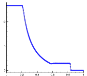
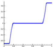
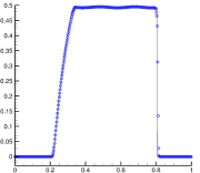
Example 2 (Riemann problem 1)

The initial data of the first 1D Riemann problem are

$$(\rho,u,p)=\begin{cases}(10,~{}0,~{}40/3),&\quad x<0.5,\\ (1,~{}0,~{}10^{-6}),&\quad x>0.5.\end{cases}$$

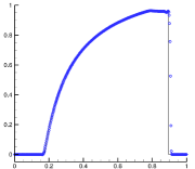
As the time increases, the initial discontinuity will be decomposed into a left-moving rarefaction wave, a contact discontinuity, and a right-moving shock wave. The rest-mass density, the velocity, and the pressure at $t=0.4$ obtained by the entropy stable schemes with $400$ are shown in Figure 1. One can see that the numerical solutions are in good agreement with the exact solutions, and the shock, the rarefaction wave, and the contact discontinuity are well captured without obvious oscillations.

(a) $\rho$

(b) $u$

(c) $p$

Figure 1: Example 2: Circles and the solid lines denote the numerical and exact solutions, respectively. $N=400,~{}t=0.4$.

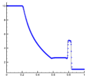
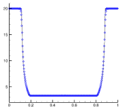
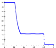
Example 3 (Riemann problem 2)

The initial data of the second 1D Riemann problem are

$$(\rho,u,p)=\begin{cases}(1,~{}0,~{}10^{3}),&\quad x<0.5,\\ (1,~{}0,~{}10^{-2}),&\quad x>0.5.\end{cases}$$ (20)

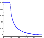
The flow pattern is similar to that of the first Riemann problem, but more extreme and difficult with a heavily curved profile for the rarefaction fan. The region between the contact discontinuity and the right-moving shock wave is very narrow so that resolving those waves is very challenging. The rest-mass density, the velocity, and the pressure at $t=0.4$ obtained by the entropy stable scheme with $400$ are shown in Figure 2. It can be seen that our scheme can still resolve the waves well, especially for the rest-mass density profile, even though small undershoot appears in the narrow region between the contact discontinuity and the right-moving shock wave.

(a) $\rho$

(b) $u$

(c) $p$

Figure 2: Example 3: Circles and the solid lines denote the numerical and exact solutions, respectively. $N=400,~{}t=0.4$.

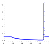
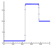
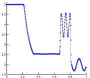
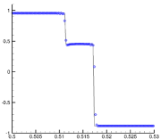
Example 4 (Riemann problem 3)

The initial data of the third 1D Riemann problem are

$$(\rho,u,p)=\begin{cases}(1,~{}0.9,~{}1),&\quad x<0.5,\\ (1,~{}0,~{}10),&\quad x>0.5,\end{cases}$$ (21)

with $\Gamma=4/3$.

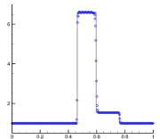
The solutions will contain a slowly left-moving shock wave, a contact discontinuity, and a fast right-moving shock wave, see Figure 3, where numerical solutions at $t=0.4$ are obtained by our entropy stable scheme with $400$ uniform cells. Our numerical solutions are in agreement with the exact solutions, although small oscillations are observed behind the left-moving shock wave like many shock-capturing methods, but they can be improved by using the adaptive moving mesh method, see [17].

(a) $\rho$

(b) $u$

(c) $p$

Figure 3: Example 4: Circles and the solid lines denote the numerical and exact solutions, respectively. $N=400,~{}t=0.4$.

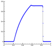
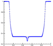
Example 5 (Riemann problem 4)

The initial data of the fourth 1D Riemann problem are

$$(\rho,u,p)=\begin{cases}(1,~{}-0.7,~{}20),&\quad x<0.5,\\ (1,~{}0.7,~{}20),&\quad x>0.5.\end{cases}$$ (22)

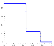
The solution of this Riemann problem consists of a left-moving rarefaction wave, a contact discontinuity, and a right-moving rarefaction wave. The rest-mass density, the velocity, and the pressure at $t=0.4$ obtained by the entropy stable scheme with $400$ are shown in Figure 4. It is seen that our entropy stable scheme can well capture the wave pattern, although in the profile of the rest-mass density, there is undershoot similar to the results in [49].

(a) $\rho$

(b) $u$

(c) $p$

Figure 4: Example 5: Circles and the solid lines denote the numerical and exact solutions, respectively. $N=400,~{}t=0.4$.

Example 6 (Density perturbation problem)

This is a more general Cauchy problem obtained by including a rest-mass density perturbation in the initial data of corresponding Riemann problem in order to test the ability of shock-capturing schemes to resolve small scale flow features, which may give a good indication of the numerical (artificial) viscosity of the scheme. The initial data are given by

$$(\rho,u,p)=\begin{cases}(5,~{}0,~{}50),&\quad x<0.5,\\ (2+0.3\sin(50x),~{}0,~{}5),&\quad x>0.5.\end{cases}$$ (23)

Figure 5 plots the numerical results at $t=0.35$ obtained by using our entropy stable scheme with $400$. The reference solution is obtained by using the first-order local Lax-Friedrichs scheme with $10000$ uniform cells. We can see that the shock wave is moving into a sinusoidal rest-mass density field, and then some smooth but complex structures are generated at the left when the shock wave interacts with the sine wave; and our entropy stable scheme can capture them well.

(a) $\rho$

(b) $u$

(c) $p$

Figure 5: Example 6: Circles and the solid lines denote the numerical and reference solutions, respectively. $N=400,~{}t=0.35$.

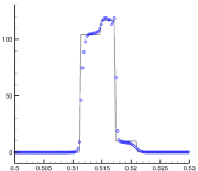
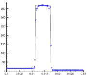
Example 7 (Blast wave interaction)

This test describes the collision of blast waves and is used to evaluate the performance of our entropy stable scheme for the flow with strong discontinuities. The initial condition is

$$(\rho,u,p)=\begin{cases}(1,~{}0,~{}10^{3}),&\quad x<0.1,\\ (1,~{}0,~{}10^{-2}),&\quad 0.1<x<0.9,\\ (1,~{}0,~{}10^{2}),&\quad x>0.9,\end{cases}$$ (24)

with inflow and outflow boundary conditions and $\Gamma=1.4$.

Figure 6 gives close-up of the solutions at $t=0.43$ obtained by using the entropy stable scheme with $4000$ uniform cells. The solutions at this time within the interval $[0.5,0.53]$ consists of two shock waves and two contact discontinuities. It can be seen that our scheme can well resolve those discontinuities and clearly capture the complex relativistic wave configuration, except for slight overshoot and undershoot of the rest-mass density and the pressure near $x=0.517$.

(a) $\rho$

(b) $u$

(c) $p$

Figure 6: Example 7: Circles and the solid lines denote the numerical and exact solutions, respectively. $N=4000,~{}t=0.43$.

4.2 Two-dimensional results

Example 8 (Accuracy test)

It is a 2D relativistic isentropic vortex problem to test the accuracy, whose detailed construction can be found in [23]. The initial rest-mass density and pressure are

$$\rho(x,y)=(1-C_{1}e^{1-r^{2}})^{\frac{1}{\Gamma-1}},\quad p=\rho^{\Gamma},$$

where

$$C_{1}=\dfrac{(\Gamma-1)/\Gamma}{8\pi^{2}}\epsilon^{2},\quad r=\sqrt{x_{0}^{2}+y_{0}^{2}},$$

$$x_{0}=x+\dfrac{\gamma-1}{2}(x+y),\quad y_{0}=y+\dfrac{\gamma-1}{2}(x+y),\quad\gamma=\dfrac{1}{\sqrt{1-w^{2}}},$$

and the initial velocities are

$$u=\dfrac{1}{1-{w(u_{0}+v_{0})}/\sqrt{2}}\left[\dfrac{u_{0}}{\gamma}-\dfrac{w}{\sqrt{2}}+\dfrac{\gamma w^{2}}{2(\gamma+1)}(u_{0}+v_{0})\right],$$

$$v=\dfrac{1}{1-{w(u_{0}+v_{0})}/\sqrt{2}}\left[\dfrac{v_{0}}{\gamma}-\dfrac{w}{\sqrt{2}}+\dfrac{\gamma w^{2}}{2(\gamma+1)}(u_{0}+v_{0})\right],$$

with

$$\quad(u_{0},v_{0})=(-y_{0},x_{0})f,\quad f=\sqrt{\dfrac{C_{2}}{1+C_{2}r^{2}}},\quad C_{2}=\dfrac{2\Gamma C_{1}e^{1-r^{2}}}{2\Gamma-1-\Gamma C_{1}e^{1-r^{2}}}.$$

This test describes a relativistic vortex moves with a constant speed of magnitude $w$ in $(-1,-1)$ direction.

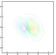
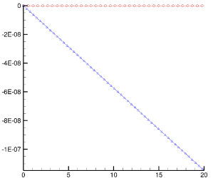
The test is computed in the domain $[-5,5]^{2}$ with $w=0.5\sqrt{2},\epsilon=5$, and periodic boundary conditions. The output time is $t=20$ so that the vortex travels and returns to the original position after a period. Table 2 lists the errors of the rest-mass density and orders of convergence. It can be clearly seen that our entropy stable scheme achieves fifth-order accuracy. Figure 7 plots the contours of the rest-mass density, and the velocities with $30$ equally spaced contour lines. The results show that due to the Lorentz contraction, the vortex becomes elliptic and the velocity in $x$- (resp. $y$-) direction is not symmetric respect to $y=0$ (resp. $x=0$) anymore. Figure 8 presents the change of the total entropy $\sum_{i,j}\eta(\bm{U}_{i,j})\Delta x\Delta y$ with respect to the time obtained by the entropy conservative scheme and the entropy stable scheme with $N_{x}=N_{y}=320$. We can see that for the entropy conservative scheme, the total entropy almost keeps conservative and for the entropy stable scheme, the total entropy decays as expected.

$N$	$\ell^{1}$ error	order	$\ell^{2}$ error	order	$\ell^{\infty}$ error	order
20	1.704e-02	-	4.982e-02	-	4.276e-01	-
40	2.886e-03	2.56	8.947e-03	2.48	7.352e-02	2.54
80	1.781e-04	4.02	6.750e-04	3.73	1.300e-02	2.50
160	4.973e-06	5.16	2.962e-05	4.51	9.425e-04	3.79
320	1.026e-07	5.60	8.240e-07	5.17	3.048e-05	4.95

Table 2: Example 8: Errors and orders of convergence in the rest-mass density at $t=20$.

(a) $\rho$

(b) $u$

(c) $v$

Figure 7: Example 8: $30$ equally spaced contour lines. $N_{x}=N_{y}=320,~{}t=20$.

Figure 8: Example 8: The change of the total entropy with respect to $t$. Circles and deltas denote the results obtained by the entropy conservative scheme and the entropy stable scheme, respectively. $N_{x}=N_{y}=320$.

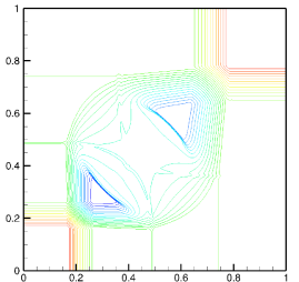
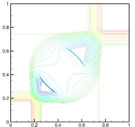
Example 9 (Riemann problem 1)

The initial data are

$$(\rho,u,v,p)=\begin{cases}(0.5,~{}0.5,-0.5,~{}5),&\quad x>0.5,~{}y>0.5,\\ (1,~{}0.5,~{}0.5,~{}5),&\quad x<0.5,~{}y>0.5,\\ (3,-0.5,~{}0.5,~{}5),&\quad x<0.5,~{}y<0.5,\\ (1.5,-0.5,-0.5,~{}5),&\quad x>0.5,~{}y<0.5.\end{cases}$$

It describes the interaction of four contact discontinuities (vortex sheets) with the same sign (the negative sign).

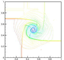
Figure 9 shows the contours of the rest-mass density and pressure logarithms with $30$ equally spaced contour lines. We can see that the four initial vortex sheets interact each other to form a spiral with the low rest-mass density around the center of the domain as time increases, which is the typical cavitation phenomenon in gas dynamics.

Figure 9: Example 9: $N_{x}=N_{y}=400$, left: $\ln\rho$, right: $\ln p$, $30$ equally spaced contour lines.

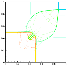
Example 10 (Riemann problem 2)

The initial data are

$$(\rho,u,v,p)=\begin{cases}(1,~{}0,~{}0,~{}1),&\quad x>0.5,~{}y>0.5,\\ (0.5771,-0.3529,~{}0,~{}0.4),&\quad x<0.5,~{}y>0.5,\\ (1,-0.3529,-0.3529,~{}1),&\quad x<0.5,~{}y<0.5,\\ (0.5771,~{}0,-0.3529,~{}0.4),&\quad x>0.5,~{}y<0.5,\end{cases}$$

which is about the interaction of four rarefaction waves.

Figure 10 plots the contours of the rest-mass density and pressure logarithms with $30$ equally spaced contour lines. The results show that those four initial discontinuities first evolve as four rarefaction waves and then interact each other and form two (almost parallel) curved shock waves perpendicular to the line $y=x$ as time increases.

Figure 10: Example 10: $N_{x}=N_{y}=400$, left: $\ln\rho$, right: $\ln p$, $30$ equally spaced contour lines.

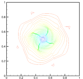
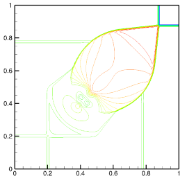
Example 11 (Riemann problem 3)

The initial data are

$$(\rho,u,v,p)=\begin{cases}(0.035145216124503,~{}0,~{}0,~{}0.162931056509027),&\quad x>0.5,~{}y>0.5,\\ (0.1,~{}0.7,~{}0,~{}1),&\quad x<0.5,~{}y>0.5,\\ (0.5,~{}0,~{}0,~{}1),&\quad x<0.5,~{}y<0.5,\\ (0.1,~{}0,~{}0.7,~{}1),&\quad x>0.5,~{}y<0.5,\end{cases}$$

where the left and bottom discontinuities are two contact discontinuities and the top and right are two shock waves.

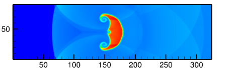
We show the contours of the rest-mass density and pressure logarithms with $30$ equally spaced contour lines in Figure 11. The initial discontinuities interact each other, and form a “mushroom cloud” around the point $(0.5,0.5)$.

Figure 11: Example 11: $N_{x}=N_{y}=400$, left: $\ln\rho$, right: $\ln p$, $30$ equally spaced contour lines.

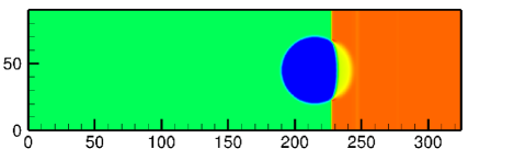
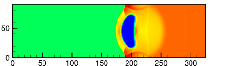
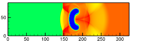
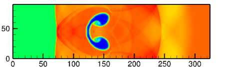
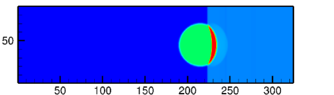
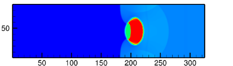
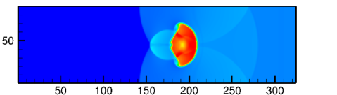
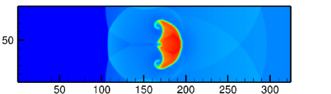
Example 12 (Shock-bubble interaction problems)

This example considers two shock-bubble interaction problems within the computational domain $[0,325]\times[-45,45]$. The detailed setup can be found in [17]. For the first problem, the initial left and right states of the planar shock wave moving left are

$$(\rho,u,v,p)=\begin{cases}(1,~{}0,~{}0,~{}0.05),&\quad x<265,\\ (1.865225080631180,-0.196781107378299,~{}0,~{}0.15),&\quad x<265,\end{cases}$$

and the state of the bubble is

$$(\rho,u,v,p)=(0.1358,~{}0,~{}0,~{}0.05),\quad\sqrt{(x-45)^{2}+(y-45)^{2}}\leq 25.$$

The setup of the second problem is the same except that the initial state of the bubble is replace with $(\rho,u,v,p)=(0.1358,~{}0,~{}0,~{}0.05)$.

Figure 12 shows the schlieren images of the rest-mass density $\rho$ of the first shock-bubble interaction problem at $t=90,180,270,360,450$ (from top to bottom) with $N_{x}=650,~{}N_{y}=180$. Figure 13 gives the schlieren images of the rest-mass density $\rho$ of the second shock-bubble interaction problem at $t=100,200,300,400,500$ (from top to bottom) with $N_{x}=650,~{}N_{y}=180$. Those plots clearly show the dynamics of the interaction between the shock waves and the bubbles, and the discontinuities and some small wave structures are also captured well by our entropy stable scheme.

Figure 12: The first problem of Example 12: the schlieren images of $\rho$ at $t=90,180,270,360,450$ from top to bottom.

Figure 13: The second problem of Example 12: the schlieren images of $\rho$ at $t=100,200,300,400,500$ from top to bottom.

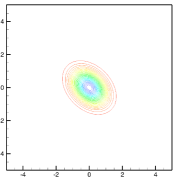
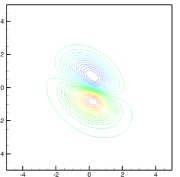
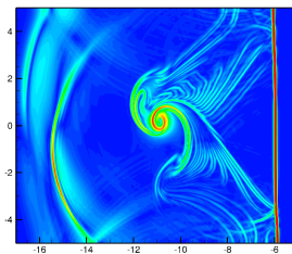
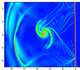
Example 13 (Shock-vortex interaction)

The final example is about the interaction between a shock wave and a vortex. The computational domain is $[-17,3]\times[-5,5]$, with reflective boundary conditions at $y=\pm 5$, inflow and outflow boundary conditions at $x=3$ and $x=-17$, respectively, and the adiabatic index is $\Gamma=1.4$. We put a similar isentropic vortex initially centered at $(0,0)$ as in Example 8, except that the vortex here is moving left with magnitude of $w=0.9$. A planar stationary shock wave with Mach number $M_{s}=1.5$ is placed at $x=-6$, which is initially far away from the vortex, thus the pre-shock state is a const state $(\rho,u,v,p)=(1,-0.9,~{}0,~{}1)$. Then from the jump condition and the Lax shock condition, we can obtain the post-shock state as

$$(\rho,u,v,p)=(4.891497310766981,-0.388882958251919,~{}0,~{}11.894863258311670).$$

Figure 14 plots the contours with $50$ equally spaced contour lines from $0$ to $1$ of $\log_{10}(1+\lvert\nabla{\rho}\rvert)$, obtained with our entropy stable scheme and the fifth-order finite difference WENO scheme with the local Lax-Friedrichs splitting. The computation is performed until $t=19$ with $N_{x}=800,~{}N_{y}=400$. We can see that, after the interaction of the vortex and the shock, the shock wave is still located at $x=-6$, and many linear and non-linear waves, and sound waves generate and propagate in the domain. Our entropy stable scheme can capture the subtle details better than the fifth-order finite difference WENO scheme with the local Lax-Friedrichs splitting.

Figure 14: Example: 13: $50$ equally spaced contours lines from $0$ to $1$ of $\log_{10}(1+\lvert\nabla{\rho}\rvert)$ at $t=19$. $M_{s}=1.5$. $N_{x}=800,~{}N_{y}=400$. Left: entropy stable scheme; right: fifth order WENO-LLF.

5 Conclusion

For the special relativistic hydrodynamic (RHD) equations, the schemes satisfying the discrete entropy condition for a convex entropy function has not been considered before. This paper has presented the high-order accurate entropy stable finite difference schemes for one- and two-dimensional special RHD equations. Those schemes are built on the entropy conservative flux and the weighted essentially non-oscillatory (WENO) technique as well as explicit Runge-Kutta time discretization. The key is to technically construct the affordable entropy conservative flux of the semi-discrete second-order accurate entropy conservative schemes satisfying the semi-discrete entropy equality for the found convex entropy pair. The entropy conservative schemes may become oscillatory near the shock wave, thus as soon as the entropy conservative flux is derived, the dissipation term can be added to give the semi-discrete entropy stable schemes satisfying the semi-discrete entropy inequality with the given convex entropy function. The WENO reconstruction for the scaled entropy variables and the high-order explicit Runge-Kutta time discretization are implemented to obtain the fully-discrete high-order schemes. Several numerical tests are conducted to validate the accuracy and the ability to capture discontinuities of our entropy stable schemes. Especially, the Shock-vortex interaction problem is designed for the first time. The results show that our schemes can achieve designed accuracy, and can well resolve the discontinuities and subtle details. In future, it will be interesting to study the physical-constraint-preserving property of the entropy stable schemes, or extend them to the relativistic magnetohydrodynamic equations.

References

- [1] D. S. Balsara, Riemann solver for relativistic hydrodynamics, J. Comput. Phys., 114 (1994), 284-297.
- [2] T. J. Barth, Numerical methods for gas-dynamics systems on unstructured meshes, in An Introduction to Recent Developments in Theory and Numerics of Conservation Laws, edited by D. Kroner, M. Ohlberger and C. Rohde, Lecture Notes in Comput. Sci. Engrg, volume 5, Berlin: Springer, 1999, 195-285.
- [3] B. Biswas and R. Dubey, Low dissipative entropy stable schemes using third order WENO and TVD reconstructions, Advan. Comput. Math., 44 (2018), 1153-1181.
- [4] T. Chen and C.-W. Shu, Entropy stable high order discontinuous Galerkin methods with suitable quadrature rules for hyperbolic conservation laws, J. Comput. Phys., 345 (2017), 427-461.
- [5] M. G. Crandall and A. Majda, Monotone difference approximations for scalar conservation laws, Math. Comp., 34 (1980), 1-21.
- [6] C. Dafermos, Hyperbolic Conservation Laws in Continuum Physics, Berlin: Springer, 2000.
- [7] W. L. Dai and P. R. Woodward, An iterative Riemann solver for relativistic hydrodynamics, SIAM J. Sci. Stat. Comput., 18 (1997), 982-995.
- [8] A. Dolezal and S. S. M. Wong, Relativistic hydrodynamics and essentially non-oscillatory shock capturing schemes, J. Comput. Phys., 120 (1995), 266-277.
- [9] F. Eulderink and G. Mellema, General relativistic hydrodynamics with a Roe solver, Astron. Astrophys. Suppl. Ser., 110 (1995), 587-623.
- [10] T. C. Fisher and M. H. Carpenter, High-order entropy stable finite difference schemes for nonlinear conservation laws: Finite domains, J. Comput. Phys., 252 (2013), 518-557.
- [11] U. S. Fjordholm, S. Mishra and E. Tadmor, Arbitrarily high-order accurate entropy stable essentially nonoscillatory schemes for systems of conservation laws, SIAM J. Numer. Anal., 50 (2012), 544-573.
- [12] U. S. Fjordholm, S. Mishra and E. Tadmor, Energy preserving and energy stable schemes for the shallow water equations, in Proceedings of Found. of Computational Mathematics, Hong Kong, 2008, edited by F. Cucker, A. Pinkus, and M. Todd, London Math. Soc. Lecture Notes Ser. 363, London: Cambridge University Press, 2009, 93-139.
- [13] U. S. Fjordholm, S. Mishra and E. Tadmor, ENO reconstruction and ENO interpolation are stable, Found. Comput. Math., 13 (2013), 139-159.
- [14] J. A. Font, Numerical hydrodynamics and magnetohydrodynamics in general relativity, Living Rev. Relativ., 11 (2008), 7.
- [15] E. Godlewski and P.-A. Raviart, Numerical Approximation of Hyperbolic Systems of Con- servation Laws, New York: Springer, 1996.
- [16] A. Harten, On a class of high-resolution TVD stable finite difference schemes, SIAM. J. Numer. Anal., 21 (1984), 1-23.
- [17] P. He and H. Z. Tang, An adaptive moving mesh method for two-dimensional relativistic hydrodynamics, Commun. Comput. Phys., 11 (2012), 114-146.
- [18] P. He and H. Z. Tang, An adaptive moving mesh method for two-dimensional relativistic magnetohydrodynamics, Comput. Fluids, 60 (2012), 1-20.
- [19] A. Hiltebrand and S. Mishra, Entropy stable shock capturing space–time discontinuous Galerkin schemes for systems of conservation laws, Numer. Math., 126 (2014), 103-151.
- [20] F. Ismail and P. L. Roe, Affordable, entropy-consistent Euler flux functions II: Entropy production at shocks, J. Comput. Phys., 228 (2009), 5410-5436.
- [21] G.-S. Jiang and C.-W. Shu, Efficient implementation of weighted ENO schemes, J. Comput. Phys., 126 (1996), 202-228.
- [22] P. G. Lefloch, J.-M. Mercier and C. Rohde, Fully discrete, entropy conservative schemes of arbitrary order, SIAM J. Numer. Anal., 40 (2002) 1968-1992.
- [23] D. Ling, J. M. Duan and H. Z. Tang, Physical-constraints-preserving Lagrangian finite volume schemes for one- and two-dimensional special relativistic hydrodynamics, arXiv: 1901.10625.
- [24] Y. Liu, C.-W. Shu and M. Zhang, Entropy stable high order discontinuous Galerkin methods for ideal compressible MHD on structured meshes, J. Comput. Phys., 354 (2018), 163-178.
- [25] J. M. Martí and E. Müller, Extension of the piecewise parabolic method to one-dimensional relativistic hydrodynamics, J. Comput. Phys., 123 (1996), 1-14.
- [26] J. M. Martí and E. Müller, Numerical hydrodynamics in special relativity, Living Rev. Relativ., 6 (2003), 7.
- [27] J. M. Martí and E. Müller, Grid-based methods in relativistic hydrodynamics and magnetohydrodynamics, Living Rev. Comput. Astrophys., 1 (2015), 3.
- [28] M. M. May and R. H. White, Hydrodynamics calculations of general-relativistic collapse, Phys. Rev., 141 (1966), 1232-1241.
- [29] M. M. May and R. H. White, Stellar dynamics and gravitational collapse, in Methods Comput. Phys., Vol. 7, edited by B. Alder, S. Fernbach, and M. Rotenberg, New York: Academic, 1967, 219-258.
- [30] M. L. Merriam, An entropy-based approach to nonlinear stability, NASA-TM-101086, 1989.
- [31] A. Mignone, T. Plewa and G. Bodo, The piecewise parabolic method for multidimensional relativistic fluid dynamics, Astron. Astrophys. Suppl. Ser., 160 (2005), 199-219.
- [32] S. Osher, Riemann solvers, the entropy condition, and difference approximations, SIAM J. Numer. Anal., 21 (1984), 217-235.
- [33] S. Osher and E. Tadmor, On the convergence of difference approximations to scalar conservation laws, Math. Comput., 50 (1988), 19-51.
- [34] T. Qin, C.-W. Shu and Y. Yang, Bound-preserving discontinuous Galerkin methods for relativistic hydrodynamics, J. Comput. Phys., 315 (2016), 323-347.
- [35] H. Ranocha, Comparison of some entropy conservative numerical fluxes for the Euler equations, J. Sci. Comput., 76 (2018), 216-242.
- [36] V. Schneider, U. Katscher, D. H. Rischke, B. Waldhauser, J. A. Maruhn and C. D. Munz, New algorithms for ultra-relativistic numerical hydrodynamics, J. Comput. Phys., 105 (1993), 92-107.
- [37] E. Tadmor, The numerical viscosity of entropy stable schemes for systems of conservation laws, I. Math. Comp., 49 (1987), 91-103.
- [38] E. Tadmor, Entropy stability theory for difference approximations of nonlinear conservation laws and related time-dependent problems, Acta. Numer., (2004), 451-512.
- [39] J. R. Wilson, Numerical study of fluid flow in a Kerr space, Astrophys. J., 173 (1972), 431-438.
- [40] K. L. Wu, Design of provably physical-constraint-preserving methods for general relativistic hydrodynamics, Phys. Rev. D, 95 (2017), 103001.
- [41] K. L. Wu, Positivity-preserving analysis of numerical schemes for ideal magnetohydrodynamics, SIAM J. Numer, Anal., 56 (2018), 2124-2147.
- [42] K. L. Wu and C.-W. Shu, A provably positive discontinuous Galerkin method for multidimensional ideal magnetohydrodynamics, SIAM J. Sci. Comput., 40 (2018), B1302-B1329.
- [43] K. L. Wu and H. Z. Tang, A direct Eulerian GRP scheme for spherically symmetric general relativistic hydrodynamics, SIAM J. Sci. Comput., 38 (2016), B458-B489.
- [44] K. L. Wu and H. Z. Tang, Admissible states and physical constraints preserving numerical schemes for special relativistic magnetohydrodynamics, Math. Mod. Meth. Appl. Sci., 27 (2017), 1871-1928.
- [45] K. L. Wu and H. Z. Tang, High-order accurate physical-constraints-preserving finite difference WENO schemes for special relativistic hydrodynamics, J. Comput. Phys., 298 (2015), 539-564.
- [46] K. L. Wu and H. Z. Tang, On physical-constraints-preserving schemes for special relativistic magnetohydrodynamics with a general equation of state, Z. Angew. Math. Phys., 69 (2018), 84.
- [47] K. L. Wu and H. Z. Tang, Physical-constraints-preserving central discontinuous Galerkin methods for special relativistic hydrodynamics with a general equation of state, Astrophys. J. Suppl. Ser., 228 (2017), 3.
- [48] K. L. Wu, Z. C. Yang and H. Z. Tang, A third-order accurate direct Eulerian GRP scheme for one-dimensional relativistic hydrodynamics, East Asian J. Appl. Math., 4 (2014), 95-131.
- [49] Z. C. Yang, P. He and H. Z. Tang, A direct Eulerian GRP scheme for relativistic hydrodynamics: one-dimensional case, J. Comput. Phys., 230 (2011), 7964-7987.
- [50] Z. C. Yang and H. Z. Tang, A direct Eulerian GRP scheme for relativistic hydrodynamics: two-dimensional case, J. Comput. Phys., 231 (2012), 2116-2139.
- [51] L. D. Zanna and N. Bucciantini, An efficient shock-capturing central-type scheme for multidimensional relativistic flows, I: hydrodynamics, Astron. Astrophys., 390 (2002), 1177-1186.
- [52] W. Q. Zhang and A. I. MacFadyen, RAM: A relativistic adaptive mesh refinement hydrodynamics code, Astrophys. J. Suppl. Ser., 164 (2006), 255-279.
- [53] J. Zhao and H. Z. Tang, Runge-Kutta discontinuous Galerkin methods with WENO limiter for the special relativistic hydrodynamics, J. Comput. Phys., 242 (2013), 138-168.