Star-planet tidal interaction and the limits of gyrochronology

Abstract

Context. Age estimation techniques such as gyrochronology and magnetochronology cannot be applied to stars that have exchanged angular momentum with their close environments. This is especially true for a massive close-in planetary companion (with a period of a few days or less) that could have been strongly impacted by the rotational evolution of the host star, throughout the stellar evolution, through the star-planet tidal interaction.

Aims. In this article, we provide the community with a reliable region in which empirical techniques such as gyrochronology can be used with confidence.

Methods. We combined a stellar angular momentum evolution code with a planetary orbital evolution code to study in detail the impact of star-planet tidal interaction on the evolution of the surface rotation rate of the star.

Results. We show that the interaction of a close-in massive planet with its host star can strongly modify the surface rotation rate of this latter, in most of the cases associated with a planetary engulfment. A modification of the surface rotation period of more than 90% can survive a few hundred Myr after the event and a modification of 10% can last for a few Gyr. In such cases, a gyrochronology analysis of the star would incorrectly make it appear as rejuvenated, thus preventing us from using this method with confidence. To try overcome this issue, we proposed the proof of concept of a new age determination technique that we call the tidal-chronology method, which is based on the observed pair $\rm P_{rot,\star}$-$\rm P_{orb}$ of a given star-planet system, where $\rm P_{rot,\star}$ is the stellar surface rotational period and $\rm P_{orb}$ the planetary orbital period.

Conclusions. The gyrochronology technique can only be applied to isolated stars or star-planet systems outside a specific range of $\rm P_{rot,\star}$-$\rm P_{orb}$. This region tends to expand for increasing stellar and planetary mass. In that forbidden region, or if any planetary engulfment is suspected, gyrochronology should be used with extreme caution, while tidal-chronology could be considered. This technique does not provide a precise age for the system yet; however, it is already an extension of gyrochronology and could be helpful to determine a more precise range of possible ages for planetary systems composed of a star between 0.3 and 1.2 $M_{\odot}$ and a planet more massive than 1 $\rm M_{jup}$ initially located at a few hundredths of au from the host star.

1 Introduction

Determining the age of a star and in substance that of a planetary system is of prime importance as it provides information about the characteristic timescale of planet formation and migration that can strongly constrain ongoing planetary models (Ida & Lin, 2008; Mordasini et al., 2009, 2012; Alibert et al., 2013). It can also be used to constrain the star-planet interaction efficiency (Lanza et al., 2011), the nature of the star (its internal structure and chemical composition) based on stellar models, and the stellar phases the planets were subject to during their evolution (Gallet et al., 2017b).

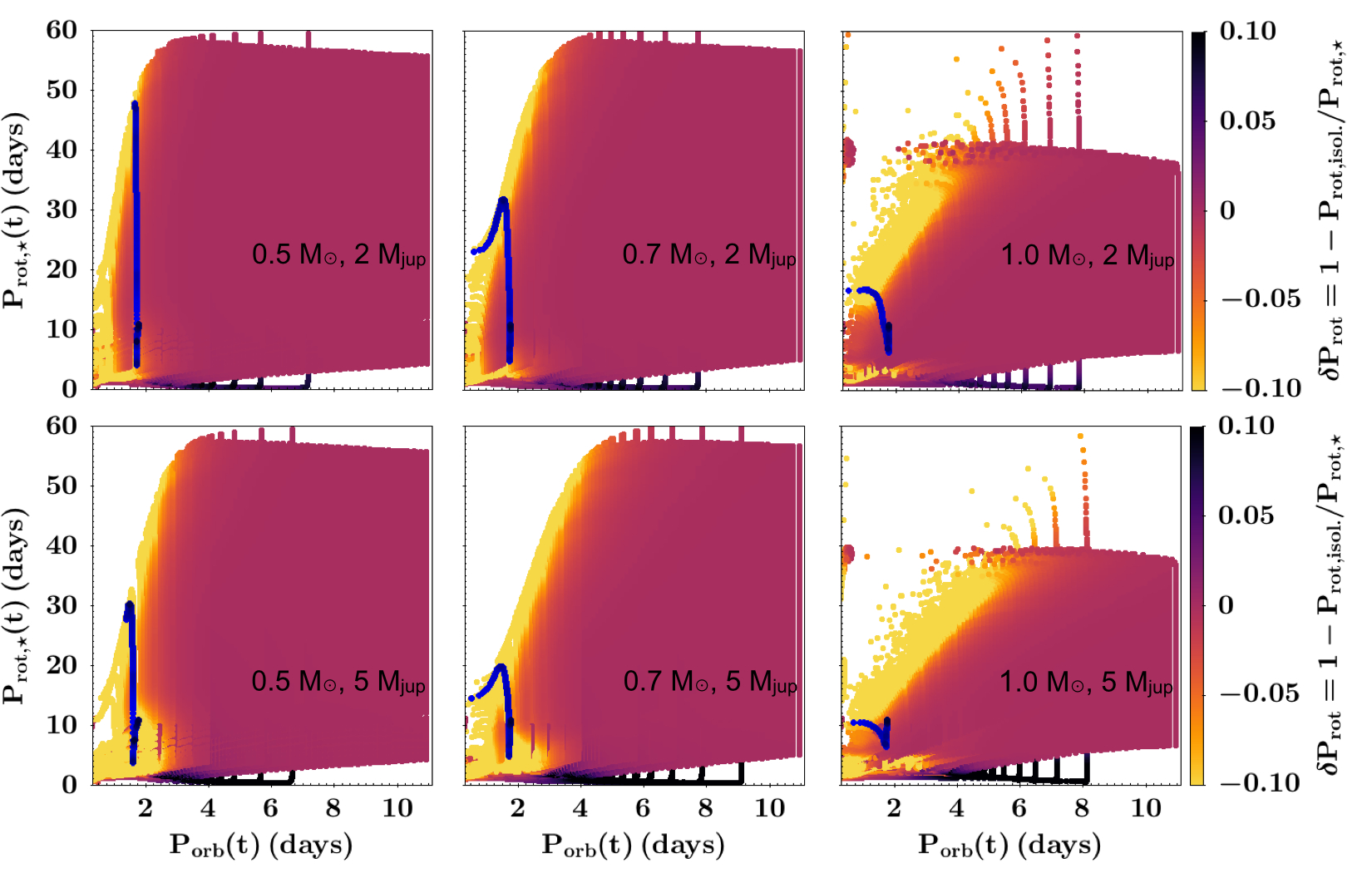
Figure 1: Evolution of $\rm P_{rot,\star}(t)$ as a function of $\rm P_{orb}(t)$ and stellar mass for a 2 $\rm M_{jup}$ (upper panel) and 5 $\rm M_{jup}$ (lower panel) planet. The color gradient corresponds to the relative rotational departure $\rm\delta P_{rot}=1-P_{rot,isol.}/P_{rot,\star}$. Only systems where the planet is still present are plotted. The blue lines (composed of plain circles) depict the evolution of a given star-planet system ($\rm P_{rot,init}=10.8$ days and $\rm SMA_{init}=30\%R_{co}$) in the $\rm P_{rot,\star}(t)-\rm P_{orb}(t)$ plane. The red area shows the domain of applicability of gyrochronology analysis.

There are three categories of age determination technique (see Soderblom 2010; Soderblom et al. 2014 and the review of Jeffries 2014 from the 2013 Evry Schatzman school):

• Semi-fundamental techniques, which rely on age-dependant phenomena that are physically well understood (e.g., nucleocosmochronometry based on the decay of long lived isotope, as is used for the Sun);

• Model-dependant techniques, such as isochrone fitting in the Hertzsprung-Russell diagram (HRD), asteroseismology, and white dwarf cooling, where the physics is mostly understood, but part of it is simplified or described using tuning parameters (e.g., the mixing length theory);

• Empirical techniques, where the understanding of the physics is qualitative and described using free parameters that are constrained using observations. They are based on the calibration of age-dependant phenomena using similar observations of stars of known age, which are then used to estimate the ages of other stars (e.g., the gyrochronology technique, see Barnes, 2007).

In the case of isolated stars (i.e., stars not impacted by interaction with the close environment during their evolution), their ages can be determined by putting them in a color-magnitude diagram (CMD) and fitting the observed sequence with stellar isochrone models. This technique obviously depends upon the stellar model used and can result in discrepancies from one model to another (Lebreton et al., 2014). Many systematics still exist, such as the effect of metallicity, the magnetic field, and the stellar model hypothesis used to produce the isochrones employed for the age determination, which prevent us from providing reliable age estimates. Additionally, to apply this technique, precise distance measurements are required in order to accurately determine the stellar parameters (i.e., luminosity and magnitudes in given bands). The Gaia mission (Gaia Collaboration et al., 2016, 2018) is revolutionizing this field by providing the community with parallax measurements of unprecedented high quality.

Empirical techniques such as gyrochronology (Barnes, 2003) and magnetochronology (Vidotto et al., 2014) also exist. Both are based on the observation that during the main-sequence (MS) phase the evolution of the surface rotation and magnetic field of a star, for a given mass, only depend on age. Provided that the stellar rotation period (respectively magnetic field strength) is measured, gyrochronology (respectively magnetochronology) analysis can be applied. However, as long as the star departs from an isolated state, i.e., if a massive planet ($\rm M_{p}>1\leavevmode\nobreak\ M_{jup}$) orbits at a close separation (less than 0.1 au) around the star, these techniques can no longer be used since star-planet tidal interaction could have modified the evolution of the surface rotation rate along the system’s evolution (Gallet et al., 2018). Consequently, the ages of numerous star-planet systems are currently not known and might appear younger than they really are. In this article we aim to provide the community with a reliable region where these empirical techniques can be used with confidence. We also present the proof of concept of a new age determination technique based on modeling the evolution of the star-planet tidal interaction, and on observation of the surface rotation rate of the host star and current location of the massive planet orbiting it.

2 Star-planet tidal interaction model

In this section we briefly describe the numerical model used in this work as well as the explored grid of initial planetary systems.

2.1 Model

In this work we combined the stellar rotational evolution model described in Gallet & Bouvier (2015) with the modified orbital evolution model used in Bolmont & Mathis (2016) (see Gallet et al., 2018, for details). The link between the two is done through the tidal dissipation induced by the gravitational interaction between the planet and the host star (see Gallet et al., 2017a). The stellar structure is provided by the stellar evolution code STAREVOL (see Amard et al., 2016, and references therein).

The aim of this coupling is to follow the evolution of a given star-planet system, using a realistic approach. This code is specifically designed for stars between 0.3 (fully convective limit) and 1.2 $\rm M_{\odot}$ (almost fully radiative limit), and for planetary systems composed of one close-in planet. The tidal dissipation formalism used in our model is based on the parametrization of Bolmont & Mathis (2016), which follows the simplified model by Ogilvie (2013). In this work, the star is assumed to be composed of a radiative core surrounded by a convective envelope both treated as regions of uniform densities. Moreover, in this work we only consider the frequency-averaged tidal dissipation and neglect the frequency response of the tides. Since these are strong assumptions, the derived frequency-averaged tidal dissipation can be in error by about one or two orders of magnitude compared to the actual tidal dissipation (Ogilvie, 2013). In Appendix C we explore the impact on the results presented in this paper of decreasing or increasing the dissipation by two orders of magnitude. We show that it does not affect our conclusion qualitatively. The model also does not include the dissipation in the planet (which is still hardly theoretically constrained) or the magnetic star-planet interaction (see Strugarek et al., 2017). Moreover, the dissipation inside the radiative core is also currently not physically described and hence not numerically included. However, for hot Jupiters and in the case of circular orbit the typical evolutionary timescale of planetary rotation rate and inclination evolution is so short ($10^{5}$ yr) that it can be safe to neglect the effects of tidal dissipation inside the planet (Leconte et al., 2010; Damiani & Mathis, 2018). Taking into account these extra dissipations could shorten the migration timescale during the MS phase and increase the departure from periods derived from wind-driven angular momentum loss, as supposed in gyrochronology analysis.

Finally, in this work we adopted an updated version of the relations from Gallet et al. (2018) that link the initial stellar conditions to the stellar mass $\rm M_{\star}$ and initial rotational period $\rm P_{rot,init.}$:

$$\tau_{\rm c-e} \approx 8.01\times\rm P_{\rm{rot,init}}^{0.69}\times\left(\displaystyle\frac{M_{\star}}{M_{\odot}}\right)^{-3.83}\rm{Myr},$$ (1)

$$\tau_{\rm disk} \approx 2.24\times\rm P_{\rm{rot,init}}^{0.61}\times\left(\displaystyle\frac{M_{\star}}{M_{\odot}}\right)^{2.24}\rm{Myr},$$ (2)

$$\rm K_{1} \approx 41.2+37.6\left(\rm\displaystyle\frac{M_{\star}}{M_{\odot}}\right)^{2}-77.3\displaystyle\frac{\rm M_{\star}}{\rm M_{\odot}}.$$ (3)

Here $\tau_{\rm c-e}$ is the coupling timescale between the radiative core and the convective envelope, $\tau_{\rm disk}$ the disk lifetime, and $\rm K_{1}$ the efficiency of the extraction of angular momentum by the stellar winds (see Gallet & Bouvier, 2013, 2015; Gallet et al., 2018).

Even if the detailed description of these quantities can be found in Gallet & Bouvier (2015), we recall the meaning of each of them. The coupling timescale $\tau_{\rm c-e}$ controls the characteristic timescale of internal angular momentum transport process. Short timescales correspond to strong coupling. We adjust these values so as to reproduce the rotational distribution of the early MS clusters (e.g., Pleiades, M50, and M35). The disk lifetime $\tau_{\rm disk}$ is the duration during which the surface rotation rate of the star is maintained constant (see Rebull et al., 2004) due to the star-disk magnetic interaction. The disk lifetime is fixed by the observation of the rotational distribution of early pre-main-sequence (PMS) clusters (e.g., Orion, NGC 6530, and NGC 2362). Finally, $\rm K_{1}$ is the wind braking efficiency that was introduced in the Matt et al. (2012) braking law. It controls the amount of angular momentum that is extracted by the stellar wind.

2.2 Grid of initial planetary systems

Using the PROBE code described in Gallet et al. (2018), we computed a grid composed of 0.5, 0.7, and 1.0 $M_{\odot}$ stars with initial rotational periods between 1 and 11 days (with $\Delta\rm P_{rot,init}$ = 0.2 days, and using a parametrization that follows Gallet & Bouvier, 2015; Gallet et al., 2018, see above). We considered 2 $\rm M_{jup}$ and 5 $\rm M_{jup}$ planets initially located at 0.1, 0.3, 0.4, 0.45, 0.5, 0.55, 0.7, 0.8, 0.92, 0.94, 0.96, 0.98, and 1.0 $\rm R_{co}$, with the corotation radius $\rm R_{co}$ given by

$$\rm R_{\rm co}=\left(\displaystyle\frac{\mathcal{G}M_{\star}}{\Omega_{\star}^{2}}\right)^{1/3}=\left(\displaystyle\frac{\mathcal{G}M_{\star}P_{\rm rot,\star}^{2}}{(2\pi)^{2}}\right)^{1/3},$$ (4)

where $\rm P_{\rm rot,\star}$ is the surface rotation period of the host star, $\mathcal{G}$ the gravitational constant, $\rm M_{\star}$ the stellar mass, and $\Omega_{\star}=2\pi/\rm P_{\rm rot,\star}$ the surface angular velocity of the host star.

In our model, we assume as initial conditions the rotation period $\rm P_{init}$ and the semi-major axis (SMA) at the time $\rm t_{0}$. The age $\rm t_{0}$ is the starting age of our simulations, and corresponds to the age at which the disk dynamically and magnetically decouples from the star. It corresponds here to the disk lifetime (i.e., the end of the disk locking phase) that occurs during the early PMS phase.

We also note that we only consider planets initially inside of the co-rotation radius. This is motivated by the fact that it is well documented (Laine et al., 2008; Laine & Lin, 2012; Chang et al., 2012; Bolmont et al., 2012; Bolmont & Mathis, 2016) that planets initially (i.e., at the disk lifetime) outside of the corotation radius tend to migrate outward, while the central star is contracting and thus accelerating toward the zero age main sequence. As a consequence, these planets will move outward, while the corotation radius moves inward. The direct effect of this opposite evolution is to drastically reduce the action of the tides induced by the planet on the stellar surface rotation rate. In this case, the central star will simply follow the same angular velocity evolution as its counterpart without a planet, which allows the use of the surface rotation rate, for example via gyrochronology (see Sect. 3), with fairly high confidence.

3 Gyrochronology and its domain of applicability

By using the numerical model and method presented in the previous section, we investigate the limit of the application of gyrochronology in the case of massive close-in planetary systems.

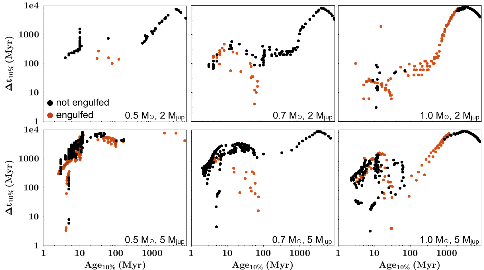
Figure 2: Duration for which the surface rotation rate of a star in a star-planet system departs by more than 10% compared to the same but isolated star (see sect. 3.1 for the definition of the variables). The black dots correspond to planets still orbiting the star, while the red dots are planets that have been engulfed.

3.1 Nomenclature and definition of the variables

Gyrochronology was initially proposed by Barnes (2003) as a technique to estimate the age of isolated stars. It is based on the behavior of the surface rotation rate of the stars between 0.3 and 1.0 $\rm M_{\odot}$ that seems to evolve as $\rm t^{-1/2}$ during the MS phase (see Skumanich, 1972).

In this section, and for the sake of clarity, we provide the definitions of numerous variables that will be used in the following:

• $\rm t_{0}$ is the starting age of our simulations. In our model it corresponds to the end of the star-disk magnetic interaction phase ($\rm\tau_{disk}$) that depends on the initial properties of the star.

• $\rm P_{init}$ is the stellar rotation period at $\rm t_{0}$.

• $\rm SMA_{init}$ is the planetary SMA at $\rm t_{0}$.

• $\rm P_{rot,isol.}$ is the rotation period of a star without a planet.

• $\rm P_{rot,\star}$ is the rotation period of a star with an orbiting planet.

• $\rm\delta P_{rot}=1-P_{rot,isol.}/P_{rot,\star}$ is the relative rotational departure between a star with and without planet.

• $\rm Age_{x\%}$ is the age at which the relative rotational departure $\rm\delta P_{rot}$ becomes greater than $\rm x\%$ (because of a planetary engulfment or strong tidal interactions).

• $\rm P_{rot,x\%}$ is the rotation period of a star at the specific age $\rm Age_{x\%}$.

• $\rm P_{orb,x\%}$ is the orbital period of a planet at the specific age $\rm Age_{x\%}$.

• $\rm P_{rot,isol.,x\%}$ is the rotation period of a star but without a planet at the specific age $\rm Age_{x\%}$. It is used as a comparison value to quantitatively extract the impact of the presence of a massive planet on the surface rotation rate of the stars.

• $\rm\Delta t_{x\%}$ is the time during which the relative rotational departure $\rm\delta P_{rot}\geq x\%$. For example, $\rm\Delta t_{0\%}$ corresponds to the time it takes for a star to return to the rotational behavior of an isolated star.

• $\rm Age_{gyro}$ is the age estimated using a gyrochronology tool and based on $\rm P_{rot,x\%}$. It corresponds to the age estimated using the observed stellar rotation period without information about the rotational history.

• $\rm Age_{gyro,isol.}$ is the “real” age of a star estimated using gyrochronology and based on $\rm P_{rot,isol.,x\%}$. It corresponds to the true gyrochronologic age of a star that has never experienced an impact of a planetary companion.

We note that $\rm Age_{gyro,isol.}$ and $\rm Age_{gyro}$ are semi-synthetic ages since they are estimated using the rotation rate provided by the numerical model and the gyrochronology tools calibrated on the observations. The difference between $\rm Age_{gyro,isol.}$ and $\rm Age_{gyro}$ highlights the possible error on the age estimation that can be introduced by the presence of a massive close-in planet. Moreover, in the case of a perfect age-$\rm P_{rot,\star}$ relationship, $\rm Age_{gyro,isol.}$ and $\rm Age_{x\%}$ should, by definition, be identical. However, since $\rm Age_{x\%}$ is directly obtained from the stellar model STAREVOL, while $\rm Age_{gyro}$ is calibrated using observations, the two ages are different (see Table 1).

In this article we used the gyrochronology calibration described in Delorme et al. (2011) that is slightly different from that proposed in Barnes (2003, 2007, 2010). In Delorme et al. (2011) the calibration of the gyrochronology is done using the SuperWASP cluster data (Pollacco et al., 2006) in addition to the properties of the Hyades cluster

$$\rm Age_{gyro}=Age_{Hyades}*(P_{rot,obs.}/P_{Hyades})^{1/0.56}\leavevmode\nobreak\ Myr,$$ (5)

where the period-color relation in the Hyades is given by

$$\rm P_{Hyades}=10.603+12.314*(J-K_{s}-0.57)\leavevmode\nobreak\ days,$$ (6)

with $\rm Age_{Hyades}=625\leavevmode\nobreak\ Myr$. The (J-$\rm K_{s}$)-mass relation is given by the YREC isochrones extracted at 600 Myr for solar metallicity stars (Z = 0.01757, see An et al., 2007).

Finally, gyrochronology analysis can only be applied to systems whose real age is older than about 100-200 Myr for a 1.0 $\rm M_{\odot}$ star and 500-600 Myr for a 0.6 $\rm M_{\odot}$ star (Barnes, 2010; Delorme et al., 2011).

3.2 Impact of tidal interaction on rotation

Figure 1 shows the evolution of $\rm P_{rot,\star}$(t) as a function of the SMA(t) expressed in orbital period $\rm P_{orb}(t)$, for the three stellar masses (0.5, 0.7, and 1.0 $M_{\odot}$), and the two planetary masses (2 $\rm M_{jup}$ and 5 $\rm M_{jup}$) considered in this work. The relation between SMA and $\rm P_{orb}$ is given by

$$\rm P_{orb}=2\pi\sqrt{\frac{\rm SMA^{3}}{\rm\mathcal{G}(M_{\star}+M_{p})}}.$$ (7)

The color gradient corresponds to the variation in $\delta\rm P_{rot}$ for each pair $[\rm P_{rot,\star}(t)-SMA(t)-M_{\star}-M_{p}]$.

Figure 1 displays the domain of validity of the gyrochronology analysis. In this figure the brightest part corresponds to the region where the star is 10% faster ($|\delta\rm P_{rot}|\geq 10\%$) than an isolated star, which corresponds to an error of about 20% on the age estimation using the gyrochronology analysis ($\rm\Omega_{\star}\propto t^{-\alpha}$, with $\alpha$ around 0.50-0.56, see Barnes, 2007; Mamajek & Hillenbrand, 2008; Delorme et al., 2011; Angus et al., 2015). This region, which depends on the stellar and planetary mass, is located in the left part of each of these plots. For the 1.0 $\rm M_{\odot}$ star, this region is positioned around $\rm P_{orb}(t)<4.2$ days (SMA(t) $\lesssim$ 0.05 au) and $\rm P_{rot}(t)$ between 10 and 50 days. Increasing the planetary mass slightly extends this region toward higher $\rm P_{orb}(t)$ (SMA(t)).

Figure 2 shows the characteristic time during which the impact of the star-planet tidal interaction on the surface rotation rate of the star remains above $\rm\delta P_{rot}$ = 10%, which corresponds to the typical systematical error of the gyrochronology analysis. If the departure $\rm\delta P_{rot}$ is above 10% during the PMS (age $\lesssim$ 100 Myr) then the characteristic timescale $\rm\displaystyle\Delta t_{10\%}$ decreases with increasing stellar mass. For all the stellar masses, the duration $\rm\displaystyle\Delta t_{10\%}$ ranges between a few tens or hundreds of Myr and several Gyr. However, the effect of the impact of the star-planet tidal interaction is visible at longer ages when the planet is engulfed during the MS phase (due to the stable internal structure of the stars during that phase).

If a planet more massive than about 1 $\rm M_{jup}$ and located below 0.1 au is detected orbiting its host star, then applying the gyrochronology would lead to a systematic underestimation of the age of the system by at least 20%. If no planets are detected, but there is a suspicion of planetary engulfment, then the gyrochronology analysis could also lead to significant systematics errors.

In some cases, the gyrochronology cannot be applied even several Gyr after the engulfment (see Fig. 2). The GJ 504 system (Fuhrmann & Chini, 2015; D’Orazi et al., 2017; Bonnefoy et al., 2018) is a striking example of the difficulty of determining the age of a given system even with the use of multiple age estimation techniques. In this case, the available techniques in the literature provide colliding results leading to either a young system (age less than 150 Myr) or an advanced system (age above 2 Gyr).

In the case of GJ 504, the error on the estimation of the age is clearly beyond the 20% error limits that we considered in the previous sections. To investigate whether the presence of a massive planet around a star can produce such a discrepancy in the age estimation, we also considered very strong star-planet interactions with $\rm\delta P_{rot}\geq 0.9$.

Table 1 shows the difference in the age estimation using a gyrochronology tool (as used in Delorme et al., 2011) between an isolated star and the same star but with a massive planet as companion. We extracted the rotation period $\rm P_{rot,90\%}$, the orbital period $\rm P_{orb,90\%}$ (when the planet is still orbiting the star), and the age $\rm Age_{90\%}$ at which the rotation of the star departs by more than 90% compared to the same but isolated star. By using $\rm P_{rot,90\%}$ and $\rm P_{rot,isol.,90\%}$, we estimated the gyrochronology ages ($\rm Age_{gyro}$ and $\rm Age_{gyro,isol.}$) of these systems so as to extract the error on the age estimation imputable to the star-planet interaction. The difference in age can reach several Gyr. While a systematic error of more than 90% on $\rm\delta P_{rot}$ only lasts a few tens or hundreds of Myr (see Table 1, $\rm\Delta t_{90\%}$), in the case of a 10% error $\rm\Delta t_{10\%}$ can reach a few Gyr (see Fig. 2). In Table 1, we list the data for the 2 $\rm M_{jup}$ and 5 $\rm M_{jup}$ planets (for $\rm\delta P_{rot}\geq$ 0.1, 0.25, 0.5, 0.75, see Appendix A).

Recently, Metcalfe & Egeland (2018) investigated the limit of gyrochronology from a more intrinsic point of view. In their paper they highlighted a possible breakdown of the gyrochronology relations for stars in their mid-MS phase due to the shutdown of their dynamo driven spin-down process. They showed that during this advanced phase, chromospheric activity should provide a more reliable age estimation than gyrochonology analysis.

Table 1: Error on the estimation of the age provided by the gyrochronology analysis for stars that have experienced a relative rotational departure greater than $|\rm\delta P|=0.9$. These data are for a 2–5 $\rm M_{jup}$ planet. The long dash “–” means that the planet is already engulfed at $\rm Age_{90\%}$. Only part of the full dataset is shown; the rest is available on demand. See Sect. 3.1 for the definition of each of these quantities. The quantities written in italics indicate ages that are estimated outside of the application range of gyrochronology.

Mass	$\rm P_{init}$	$\rm SMA_{init}$	$\rm Age_{90\%}$	$\Delta t_{90\%}$	$\rm P_{rot,90\%}$	$\rm P_{orb,90\%}$	$\rm P_{rot,isol.,90\%}$	$\rm Age_{gyro}$	$\rm Age_{gyro,isol.}$
($M_{\odot}$)	(days)	(au)	(Myr)	(Myr)	(days)	(days)	(days)	(Myr)	(Myr)
0.5	4.60	0.0236	782/74	100/268	6.40/0.85	–/0.1647	13.24/1.87	159/4	583/18
0.5	5.00	0.0250	722/66	100/296	6.79/0.86	–/0.1641	13.31/2.03	177/4	588/21
0.5	5.40	0.0239	1052/98	150/284	7.81/1.05	–/0.1653	16.13/2.51	227/6	830/30
0.5	6.00	0.0231	2002/102	250/320	11.14/1.19	–/0.1666	22.85/2.78	428/8	1545/36
0.5	8.60	0.0196	6203/10	750/173	14.64/2.80	0.2642/0.1650	41.32/6.31	697/36	4450/155
0.7	5.80	0.0224	763/66	41/78	2.79/2.06	–/0.1610	13.03/4.68	42/24	650/105
0.7	7.40	0.0198	622/7	42/56	2.78/2.90	–/–	12.87/6.08	41/44	636/167
0.7	7.60	0.0202	985/8	70/57	7.45/2.68	–/–	16.07/5.88	239/39	946/157
0.7	7.80	0.0205	1355/11	100/56	8.33/2.32	–/–	18.92/5.38	292/30	1266/134
0.7	8.00	0.0209	1755/21	100/50	9.51/1.48	–/–	21.91/4.03	370/13	1645/80
0.7	8.20	0.0212	2155/165	150/100	11.94/4.80	–/–	24.71/10.41	557/109	2039/435
0.7	8.80	0.0222	3456/946	400/160	16.90/8.09	–/–	33.09/16.37	1034/278	3435/978
0.7	9.00	0.0226	3906/1206	550/200	17.95/8.78	–/–	35.08/18.34	1152/321	3812/1198
0.7	10.00	0.0242	7156/2656	1100/600	18.99/13.37	0.2643/0.1607	47.04/27.76	1274/681	6437/2511
0.7	10.40	0.0248	8707/3407	1500/900	19.48/14.35	0.2642/0.1575	50.55/32.55	1333/773	7319/3335
1.0	4.00	0.0222	491/33	14/16	1.70/1.92	–/–	7.00/3.81	38/48	482/162
1.0	5.00	0.0258	2256/22	100/12	8.26/1.01	–/–	17.78/2.98	647/15	2544/105
1.0	5.00	0.0286	1506/102	50/24	7.28/2.31	–/–	14.08/4.51	516/66	1676/220
1.0	6.00	0.0194	178/14	9/15	1.65/2.19	–/–	5.59/4.26	36/61	322/198
1.0	6.00	0.0323	5407/21	800/12	13.96/0.96	–/–	26.81/3.79	1652/14	5295/161
1.0	7.00	0.0322	6808/4208	1150/1500	15.91/12.37	–/–	30.30/23.79	2085/1330	6588/4275
1.0	7.00	0.0215	706/186	22/22	1.71/0.34	–/–	9.21/6.09	39/2	785/375
1.0	8.00	0.0313	6309/3759	900/1150	15.07/11.56	–/–	28.97/22.27	1892/1179	6078/3800
1.0	8.00	0.0235	1459/569	50/40	6.97/4.15	–/–	13.68/8.67	477/189	1591/705
1.0	9.00	0.0339	7710/5060	1150/1800	17.01/13.47	–/–	32.78/25.74	2348/1550	7580/4922
1.0	9.00	0.0254	2460/1160	150/50	9.38/4.78	–/–	17.93/12.08	812/243	2581/1274
1.0	10.00	0.0363	8811/6261	1300/2200	18.97/14.91	–/–	36.37/28.57	2856/1857	9129/5931
1.0	11.00	0.0290	4912/2662	400/400	12.64/9.34	–/–	24.91/18.37	1383/805	4642/2694

4 Tidal-chronology

Following the work of Gallet et al. (2018) we developed a new age estimation technique based on the measurement of the surface rotation rate of the star and the location of the planet around it. It relies on the fact that the star-planet interaction produces a rotation cycle that can be used to estimate the age of a given close-in system. The four steps of this cycle are as follows:

• 1) The system starts its evolution with an initial condition ($\rm P_{rot,init}$-$\rm SMA_{init}$);

• 2) Given the value of the initial rotation rate of the star and its internal structure at the initial time $t_{0}$, the efficiency ¡$\mathcal{D}$¿_ω of the dissipation of the star is estimated;

• 3) The value ¡$\mathcal{D}$¿_ω of the dissipation determines the orbital evolution of the planetary companion;

• 4) The planetary orbital evolution then modifies the surface rotation rate of the star.

The star-planet system starts again at the first step with a new pair $\rm P_{rot}$-$\rm SMA$.

Since the rate of the evolution of the SMA strongly depends on its value (see Eqs. 3-6 in Gallet et al., 2018), a given observed pair $\rm P_{\rm rot,\star}(\rm t)$-$\rm{SMA(t)}$ is thus only produced for a small range of possible ages and initial conditions, as long as the observed rotational period of the star is longer than 10 days (see Sect. 4.2). As in gyrochronology, for a rotational period below 10 days, which corresponds to a system younger than about 100 Myr, the tidal-chronology technique will provide degenerated solutions.

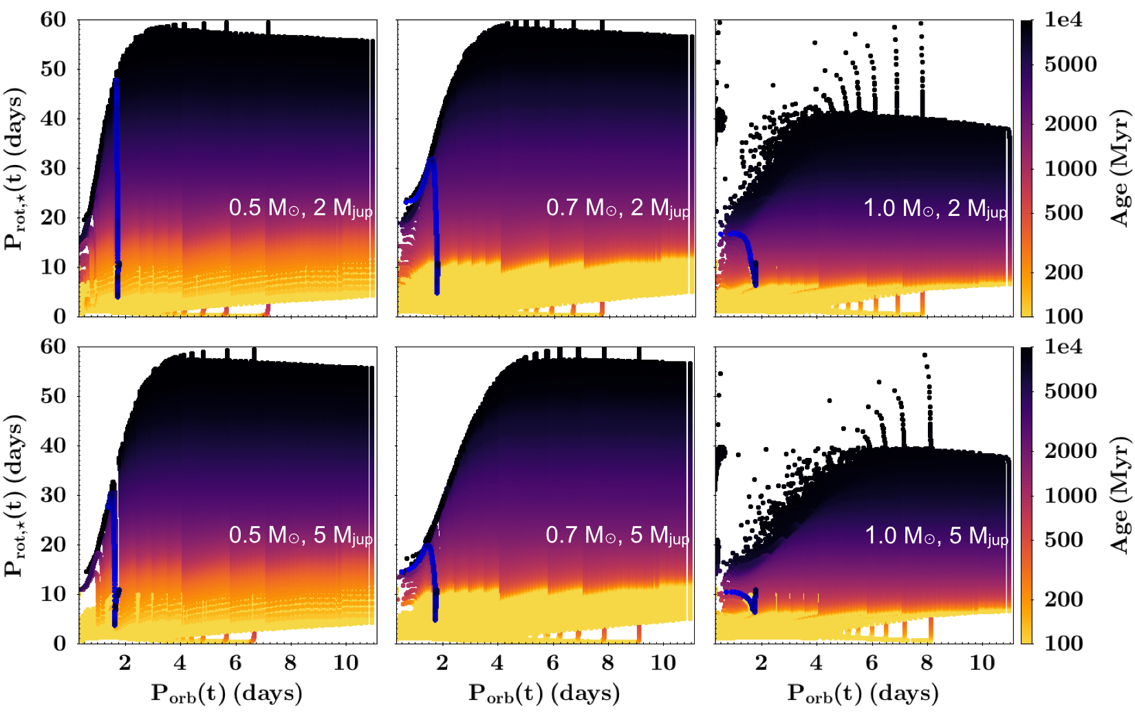
Figure 3: Synthetic $\rm P_{\rm rot,\star}$(t) and $\rm P_{orb}(t)$ estimated for a system composed of a 0.5, 0.7, and 1.0 $M_{\odot}$ star around which orbits a 2 $M_{\rm jup}$ planet (upper panel) and a 5 $M_{\rm jup}$ planet (lower panel). $\rm P_{rot,init}$ = 1-11 days (with $\Delta\rm P_{rot,init}$ = 0.2 days) and $\rm SMA_{init}$ is between 0.1 and 1.0 $\rm R_{co}$ (Gallet et al., 2018). The color gradient indicates the age (in Myr) at which the pair $\rm P_{\rm rot,\star}(t)-P_{orb}(t)$ is extracted. Only planetary systems where the planet is still orbiting the star are plotted. The blue lines (composed of plain circles) depict the evolution of a given star-planet system ($\rm P_{rot,init}=10.8$ days and $\rm SMA_{init}=30\%R_{co}$) in the $\rm P_{rot,\star}(t)-\rm P_{orb}(t)$ plane.

4.1 Description of the tidal-chronology technique

To determine the age of a planetary system we thus computed a grid of star-planet system evolutions composed of a star with $\rm P_{\rm rot,init}$ between 1 and 11 days and a planet’s initial SMA between 0.1 and 1.0 $R_{\rm co}$, for the given stellar and planetary mass that match the observed system’s properties.

We chose to express the initial SMA as a function of $R_{\rm co}$, rather than fixing the range of initial planetary orbits, so as to ensure a good coverage of the initial conditions for which the planet orbits inward ($\rm{SMA}_{\rm init}\leq R_{\rm co}$, $1.8\times 10^{-3}\rm<SMA_{init}(au)<0.09$). In the case of outward migration, the surface rotation rate of the star is less impacted by the star-planet tidal interaction.

We then explored the grid so as to extract age at which the observed pair $\rm P_{\rm rot,obs}$-$\rm SMA_{obs}$ is retrieved. The resulting grid is composed of 714 rotational-orbital evolutions (51 initial rotational periods $\times$ 14 initial SMAs) for each star-planet system. We finally estimate the departure of the observed pair $\rm P_{\rm rot,obs}$-$\rm SMA_{obs}$ to each of the $\rm P_{\rm rot,\star}$-$\rm SMA_{\star}$ pairs from the grid using the expression

$${S^{2}=\frac{(\rm SMA_{\rm\star}-\rm SMA_{\rm obs})^{2}}{\rm\sigma_{\rm SMA_{obs}}^{2}}+\frac{(\rm P_{\rm orb,\star}-\rm P_{\rm orb,obs})^{2}}{\rm\sigma_{\rm P_{orb,obs}}^{2}},}$$ (8)

where $\displaystyle\sigma_{\rm SMA_{obs}}$ and $\displaystyle\sigma_{\rm P_{orb,obs}}$ are the standard deviation of the observed $\rm SMA_{obs}$ and $\rm P_{orb,obs}$.

We also applied a 3D interpolation method using the Python-SciPy griddata routine (to interpolate unstructured 3D data, see Jones et al., 2001).

4.2 Limits, degeneracies, and framework of the tidal-chronology

To investigate the degeneracies of this technique we considered a 0.5, 0.7, and 1.0 $M_{\odot}$ stars and a 2 and 5 $M_{\rm jup}$ planets and computed a grid composed of $\rm P_{rot,init}$= 1-11 days (with $\Delta\rm P_{rot,init}$ = 0.2 days) and $\rm SMA_{init}=$ 0.1, 0.3, 0.4, 0.45, 0.5, 0.55, 0.7, 0.8, 0.92, 0.94, 0.96, 0.98, and 1.0 $\rm R_{co}$ (see Gallet et al., 2018).

Figure 3 shows $\rm P_{\rm rot,\star}$(t) as a function of $\rm P_{orb}$(t), $M_{\star}$, and $\rm M_{p}$, and displays the age as a color gradient. In this figure, $\rm P_{orb}$(t) is between 0.5 and 12 days and $\rm P_{rot,\star}$(t) between 0 and 50 days. It shows that the solutions are indeed degenerated when using only $\rm P_{\rm rot,\star}$ or SMA, but that they are lifted when using both quantities simultaneously. Additionally, the information whether the planet is still orbiting the star adds another criterion and helps remove these degeneracies.

Figure 3 shows that the age linearly increases for increasing $\rm P_{\rm rot,\star}$(t) and highlights that for $\rm P_{\rm rot}(\rm t)\gtrsim 5$ days the degeneracy in the estimation of the age is lifted when using the information about SMA(t). With Fig. 4 we can see that the age dispersion is below 10% for most of the $\rm P_{\rm rot,\star}$-$\rm SMA$ space. The degeneracy of the technique is thus quite low and might be a concern only for young systems with ages less than about 100 Myr (which are also beyond the traditional gyrochronology application range) that globally correspond to systems in which $\rm P_{\rm rot}(\rm t)$ $\lesssim$ 10 days. The degeneracy is mainly due to the high temporal resolution of the models during the PMS that display almost identical pairs $\rm P_{\rm rot}(\rm t)-SMA(t)$ for slightly different ages.

The evolution of the star-planet systems in Fig. 3 starts from the bottom of the $\rm P_{\rm rot,\star}$(t)-$\rm P_{orb}$(t) space, between 1.8$\times 10^{-3}$ au ($\rm P_{\rm rot,init}$ = 1 day, $\rm SMA_{init}$ = 0.1 $\rm R_{co}$) and 0.09 au ($\rm P_{\rm rot,init}$ = 11 days, $\rm SMA_{init}$ = $\rm R_{co}$) and $\rm P_{\rm rot,init}$ = 1-11 days. Without planetary migration, the evolution of a star-planet system is depicted by a straight line transiting from the brightest (age $\approx$ 100 Myr) to the darkest (age ¿ 1 Gyr) parts of the figure. It concerns star-planet systems in which the planet is initially located around $\rm R_{co}$.

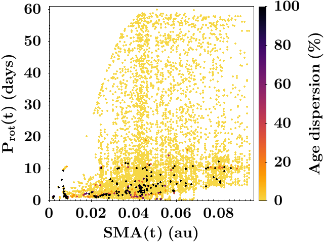
Figure 4: Randomly selected $\rm P_{\rm rot,\star}$(t)-$\rm SMA$(t) pairs (see text) with their associated age dispersion $\rm(t_{max}-t_{min})/t_{min}$.

Figure 4 shows the age dispersion for given $\rm P_{\rm rot,\star}$(t)-$\rm SMA$(t) pairs. It highlights the small degeneracy of the tidal-chronology technique when determining the age of a given planetary system from its observed $\rm P_{\rm rot,\star}$(t)-$\rm SMA$(t) pair. In Appendix B we explore the impact of the precision of $\rm P_{\rm rot,\star}$ on the degeneracy of the technique.

To produce this figure we first bin the $\rm P_{\rm rot,\star}$-$\rm SMA$ space using the classical errors on $\rm P_{\rm rot,\star}$ and $\rm SMA$: $\Delta\rm P_{\rm rot,\star}=0.001$ days (Howell et al., 2014) and $\Delta\rm SMA=0.00018$ au (Hellier et al., 2011). Given the range of $\rm P_{\rm rot,\star}$ and $\rm SMA$ of our models, this binning produced an image composed of 30 million pixels.

To allow a fast exploration of the parameter space, we then randomly selected 10000 pairs and performed a loop over the whole dataset of models so as to look at the age range, i.e., the minimum and maximum age $\rm t_{min}$ and $\rm t_{max}$, associated with each of these random pairs. We finally estimated the age dispersion $(\rm t_{max}-t_{min})/\rm t_{min}$ associated with each of these pairs and plot them in Fig. 4.

In the case of migrating planets, the evolution of star-planet systems in the $\rm P_{\rm rot,\star}$(t)-$\rm P_{orb}$(t) space depends on their initial conditions. As the star evolves, its surface rotation rate is impacted by the inward migration of the planet. The star-planet system thus moves toward smaller SMA ($\rm P_{orb}$) and rotation period (if the acceleration torque produced by the planet is stronger than the braking torque of the stellar winds or the PMS contraction torque, see the blue tracks in Fig. 1).

The hypothesis of this paper implies that the orbit of the planet is initially circular and coplanar, and remain so, with respect to the equator of the star during the whole stellar evolution. The results above and the tidal-chronology technique are hence only valid within this framework. Moreover, since we simply present the proof of concept of such a technique, for now, the tidal-chronology should be used with caution and in addition to other age determination tools. In the future, and with the increase in the completeness and complexity of our tidal dissipation modeling, we hope that this technique will be reliable enough to derive reliable stellar ages by itself.

In this paper, and because of the nature of the tidal dissipation formalism we use, we only consider isolated star-planet systems composed of one planet that orbits one star because the model that we use does not allow us to follow the evolution of multiplanetary systems. Hence, we do not consider Kozai-Lidov resonance (Kozai, 1962; Lidov, 1962), which is present in n-body systems (with n ¿ 3) for a given body with an orbital inclination greater than 39^∘. Finally, we also mention the work of Wu & Lithwick (2011) on secular chaos in the evolution of the properties of almost coplanar multiplanetary systems. They pointed out that strong variations in the orbits of the planets can occur in these kind of system on timescales ranging from a few tens of Myr to a few Gyr.

4.3 Observational case: WASP-43

To extract the order of magnitude of the difference in age estimation between standard gyrochronology and tidal-chronology, we decided to apply and illustrate our technique on a specific planetary system, namely WASP-43, for which the rotation rate of the star is well known, as is the location of the orbiting planet.

WASP-43 is a K7V star (corresponding to 0.717 $\pm$ 0.025 $\rm M_{\odot}$), with $T_{\rm eff}=4520\pm 120$ K and solar metallicity [Fe/H] = 0.01 $\pm$ 0.012. Around this star orbits a 2.052 $\rm M_{\rm jup}$ planet (Hellier et al., 2011). The rotation period of the star is estimated at 15.6 $\pm$ 0.4 days and the planet is observed at a distance of 0.01526 au from the star. The standard deviations for WASP43 are $\displaystyle\sigma_{\rm SMA_{obs}}=0.00018$ au and $\displaystyle\sigma_{\rm P_{orb,obs}}=0.4$ days (Hellier et al., 2011). The system’s eccentricity is very low (0.0035, see also Bonomo et al., 2017, for other estimations of hot-Jupiter system parameters) and the inclination is quite high (82 degree), which allows us to apply, at the first order, the dynamical tides formalism of our numerical code.

It is not certain, however, that the eccentricity was this low during the whole system evolution. The main effect of increasing the eccentricity of the systems on the evolution of the dynamical tide is the excitation of multiple frequencies, which can boost the tidal dissipation and thus the evolution of the SMA. These effects are expected to be the strongest during the PMS phase (Emeline Bolmont, private communication). The same kind of effect can appear for the equilibrium tide. High eccentricity can lead to an increase in the transfer of angular momentum from the planetary orbit to the stellar rotation, which implies a faster rate of acceleration of the central star.

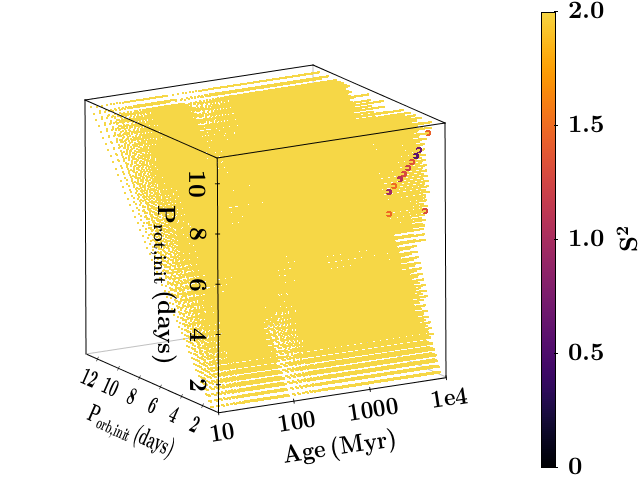
Figure 5: Map of $\rm S^{2}$ for the WASP-43 system as a function of time, $\rm P_{\rm rot,init}$, and $\rm P_{orb,init}$.

Figure 5 shows (as a color gradient) the value of $\rm S^{2}$ as a function of time, $\rm{SMA}_{init}$, and $\rm P_{\rm rot,init}$. Using the gyrochronology technique based on the Barnes (2007) calibration, the age of WASP-43 was estimated at 400 Myr by Hellier et al. (2011). With the more recent calibrations of Barnes (2010) and Delorme et al. (2011), a gyrochronologic age of 0.9-1.0 Gyr can be estimated for WASP43. Using our tidal-chronology technique, the most probable solutions suggest an older system with an age between 2.4 and 9.2 Gyr (see Fig. 5) with a minimum $\rm S^{2}$ of 0.58 at 5.85 Gyr. A 3D linear interpolation of the observed pair leads to an age estimation of 3.5${\pm 1.1}$ Gyr, which is consistent with our $S^{2}$ exploration. The difference between the two estimated ages is also consistent with the global age shift that can be introduced by a massive planet (see Table 1).

4.4 Impact of the high uncertainty on the tidal dissipation intensity factor

Since the efficiency of the tidal dissipation is currently not well constrained in theory, we decided to explore to what extent the tidal-chronology technique depends upon this intensity. In this section, we thus investigate the impact of a 2 $\rm M_{jup}$ planet on the surface rotation rate of a 0.7 $\rm M_{\odot}$ star and consider a tidal dissipation intensity two orders of magnitude higher (¡$\rm{\mathcal{D}}$¿_∗100) or lower (¡$\rm{\mathcal{D}}$¿_/100) than the averaged values (¡$\rm{\mathcal{D}}$¿) from Gallet et al. (2017b).

The results are summarized in Tables 6 and 7. They show that the main effect of increasing (decreasing) the global intensity of the tidal dissipation is to increase (decrease) the migration timescale of the planet. The overall conclusions of the paper, however, are not impacted by this tidal-dissipation efficiency effect. More specifically, the intensity of the effect of a given planet on the surface rotation rate of its central star is not impacted by a change in tidal-dissipation efficiency.

The observed properties of the WASP43 system are retrieved (in the case of a 0.7 $\rm M_{\odot}$ and a 2 $\rm M_{jup}$) at 3.0 Gyr when using the normal tidal dissipation evolution. When using the reduced efficiency, the age estimation increases to 5.3 Gyr, which is expected given that the tidal timescale is increased when the overall dissipation is reduced. Interestingly, with the increased tidal dissipation, the age estimation is not shorter than that estimated using the normal dissipation, and is evaluated at 4.0 Gyr. With this increased dissipation, most of the close-in planets fall earlier into the central star. Since the main property of WASP-43 is that an orbiting planet is observed, these systems (i.e., the ones without a remaining planet) are discarded, and are no longer used for age estimation. As a consequence, the observed properties of the WASP-43 are retrieved at greater age compared to the normal tidal dissipation age.

5 Conclusion

We showed that gyrochronology can be applied, with an error on the age estimation below 20%, to massive close-in planetary systems where the orbital period of the massive planet is greater than $\rm P_{orb}\approx 4$ days (for a 1 $\rm M_{\odot}$ star and a planet less massive than 5 $\rm M_{jup}$). In the range of initial planetary systems’ conditions that we explored in this article, we highlighted that this limit increase with the stellar and planetary mass.

In this work, we determined that in the case of planetary engulfment, the effect of the transfer of angular momentum from the planetary orbit to the stellar rotation could persist on a characteristic timescale of a few hundred Myr to a few Gyr (see Table 1 and Fig. 2). We also investigated more dramatic events where the surface rotation rate of the star departs by more than 90% from the rotation of the same but isolated star. We pointed out that in these scenarios the estimation of the age with the gyrochronology technique can lead to an age that is, in some cases, younger than several Gyr compared to the true age. Such massive departures can survive for tens of Myr to a few hundred Myr after the event, which most of the time is linked to a planetary engulfment, and can cause a more moderate but lasting 10% departure for up to a few Gyr. Provided the star experienced a planetary engulfment in its recent past, this effect could explain the bimodal age estimation of planetary systems such as GJ 504 (Fuhrmann & Chini, 2015; D’Orazi et al., 2017; Bonnefoy et al., 2018) for which two incompatible ages are found, depending on the technique employed.

Gyrochronology, if combined with other techniques, can be a convenient and rapid tool for age determination; however, it should be kept in mind that the evolution of the stellar rotation could have been strongly modified by external torques such as star-planet tidal interaction. To overcome this issue, we proposed a proof of concept of a new age determination technique that can be applied to such close-in planetary systems: tidal-chronology. This technique is based on the uniqueness of the path followed by a planetary system on the $\rm P_{\rm rot,\star}$(t)-$\rm P_{orb}$(t) plane.

However, though an improvement over gyrochronology, the numerical and physical description of the tidal dissipation in stellar and planetary interior is currently not good enough to use this age estimation alone; it should be considered with caution and in combination with other age determination techniques. In this work we do not include the dissipation in the planet (which is still hardly theoretically constrained) nor the magnetic star-planet interaction (see Strugarek et al., 2017). The dissipation inside of the radiative core is also currently not physically described, and hence not numerically included. While the magnetic star-planet interaction torque is only present during the early PMS phase, the extra dissipations (from the planet, from the radiative core, and from taking into account the frequency response of the tidal dissipation) could shorten the migration timescale during the MS phase, and consequently reduce the estimated age of the system. The behavior of these additional mechanisms is unfortunately not yet known, which prevents us from predicting their possible effect and impact on the conclusion reached in Sect. 3. However, while the quantitative results from Sect. 3 might change, we expect its general conclusion to remain the same.

Within these limitations, we developed a promising technique that will benefit the community when all aspects of tidal and magnetic star-planet interactions are included in angular momentum evolution models.

Appendix A Exploration of different $|\rm\delta P|$?

Tables 2, 3, 4, and 5 show the same data as in Table 1, but for different values of $|\rm\delta P|$= 10, 25, 50, and 75 %.

Table 2: Same as Table 1, but for $|\rm\delta P|=0.1$.

Mass	$\rm P_{init}$	$\rm SMA_{init}$	$\rm Age_{10\%}$	$\Delta t_{10\%}$	$\rm P_{rot,10\%}$	$\rm P_{orb,10\%}$	$\rm P_{rot,isol.,10\%}$	$\rm Age_{gyro}$	$\rm Age_{gyro,isol.}$
($M_{\odot}$)	(days)	(au)	(Myr)	(Myr)	(days)	(days)	(days)	(Myr)	(Myr)
0.5	6.00	0.0231	1902/102	2950/3600	13.13/1.19	0.2641/0.1666	22.26/2.78	575/8	1474/36
0.5	8.60	0.0196	6203/10	6000/4693	14.64/2.80	0.2642/0.1650	41.32/6.31	697/36	4450/155
0.7	5.00	0.0229	163/29	180/1724	6.04/1.30	0.2642/0.1581	7.08/1.97	165/11	219/22
0.7	6.00	0.0258	524/38	260/2116	9.03/1.27	0.2643/0.1651	10.99/2.38	338/10	480/31
0.7	7.00	0.0286	4155/35	8050/2770	17.94/1.30	0.2635/0.1630	36.71/2.92	1151/11	4133/45
0.7	8.00	0.0209	1405/14	2300/2991	15.32/3.36	0.2643/0.1621	19.36/4.74	869/58	1318/107
0.7	9.00	0.0226	3856/966	8050/3340	18.46/11.53	0.2639/0.1623	34.86/16.63	1211/523	3770/1006
0.7	10.00	0.0242	7156/2656	5050/7650	18.99/13.37	0.2643/0.1607	47.04/27.76	1274/681	6437/2511
1.0	4.00	0.0222	425/19	100/44	5.77/1.84	–/–	6.49/2.20	341/44	421/61
1.0	5.00	0.0258	1406/22	4250/904	12.22/1.01	–/–	13.57/2.98	1301/15	1570/105
1.0	6.00	0.0291	3957/1757	8250/6850	16.87/11.95	0.2623/0.2104	23.00/15.13	2316/1250	4027/1906
1.0	7.00	0.0322	6058/3708	6150/8500	18.85/13.64	0.2606/0.2857	28.28/22.34	2822/1583	5825/3822
1.0	8.00	0.0352	7459/5459	4750/6750	21.56/14.92	0.2530/0.3451	32.24/26.66	3588/1860	7360/5241
1.0	9.00	0.0339	6710/4560	5500/7650	20.61/14.57	0.2480/0.3128	30.03/24.23	3311/1781	6484/4418
1.0	10.00	0.0363	7711/5861	4500/6350	22.78/15.75	0.2562/0.3668	32.66/27.50	3958/2047	7532/5542
1.0	11.00	0.0290	3312/1162	8900/7450	17.13/11.11	0.2599/–	20.60/12.26	2380/1097	3306/1310

Table 3: Same as Table 1, but for $|\rm\delta P|=0.25$.

Mass	$\rm P_{init}$	$\rm SMA_{init}$	$\rm Age_{25\%}$	$\Delta t_{25\%}$	$\rm P_{rot,25\%}$	$\rm P_{orb,25\%}$	$\rm P_{rot,isol.,25\%}$	$\rm Age_{gyro}$	$\rm Age_{gyro,isol.}$
($M_{\odot}$)	(days)	(au)	(Myr)	(Myr)	(days)	(days)	(days)	(Myr)	(Myr)
0.5	6.00	0.0231	1902/102	800/1150	13.13/1.19	0.2641/0.1666	22.26/2.78	575/8	1474/36
0.5	8.60	0.0196	6203/10	5200/1393	14.64/2.80	0.2642/0.1650	41.32/6.31	697/36	4450/155
0.7	5.00	0.0229	223/29	80/514	5.77/1.30	–/0.1581	7.56/1.97	152/11	246/22
0.7	6.00	0.0258	564/38	160/626	8.87/1.27	–/0.1651	11.33/2.38	327/10	506/31
0.7	7.00	0.0286	4155/35	3550/1020	17.94/1.30	0.2635/0.1630	36.71/2.92	1151/11	4133/45
0.7	8.00	0.0209	1405/14	600/1091	15.32/3.36	0.2643/0.1621	19.36/4.74	869/58	1318/107
0.7	9.00	0.0226	3856/966	3300/1190	18.46/11.53	0.2639/0.1623	34.86/16.63	1211/523	3770/1006
0.7	10.00	0.0242	7156/2656	5050/3450	18.99/13.37	0.2643/0.1607	47.04/27.76	1274/681	6437/2511
1.0	4.00	0.0222	465/21	40/34	5.33/1.62	–/–	6.80/2.15	296/35	457/59
1.0	5.00	0.0258	1806/22	1650/76	12.39/1.01	–/–	15.59/2.98	1335/15	2011/105
1.0	6.00	0.0291	3957/1757	4550/3600	16.87/11.95	0.2623/0.2104	23.00/15.13	2316/1250	4027/1906
1.0	7.00	0.0322	6058/3708	5450/5050	18.85/13.64	0.2606/0.2857	28.28/22.34	2822/1583	5825/3822
1.0	8.00	0.0352	7459/5459	4750/5850	21.56/14.92	0.2530/0.3451	32.24/26.66	3588/1860	7360/5241
1.0	9.00	0.0339	6710/4560	5500/5750	20.61/14.57	0.2480/0.3128	30.03/24.23	3311/1781	6484/4418
1.0	10.00	0.0363	7711/5861	4500/6350	22.78/15.75	0.2562/0.3668	32.66/27.50	3958/2047	7532/5542
1.0	11.00	0.0290	3612/1712	4700/3550	17.04/11.77	–/–	21.46/14.72	2356/1218	3557/1815

Table 4: Same as Table 1, but for $|\rm\delta P|=0.50$.

Mass	$\rm P_{init}$	$\rm SMA_{init}$	$\rm Age_{50\%}$	$\Delta t_{50\%}$	$\rm P_{rot,50\%}$	$\rm P_{orb,50\%}$	$\rm P_{rot,isol.,50\%}$	$\rm Age_{gyro}$	$\rm Age_{gyro,isol.}$
($M_{\odot}$)	(days)	(au)	(Myr)	(Myr)	(days)	(days)	(days)	(Myr)	(Myr)
0.5	5.00	0.0250	682/66	200/516	8.04/0.86	0.2642/0.1641	13.02/2.03	239/4	566/21
0.5	6.00	0.0231	1902/102	500/420	13.13/1.19	0.2641/0.1666	22.26/2.78	575/8	1474/36
0.5	8.60	0.0196	6203/10	1950/293	14.64/2.80	0.2642/0.1650	41.32/6.31	697/36	4450/155
0.7	5.00	0.0229	263/29	40/94	2.55/1.30	–/0.1581	7.88/1.97	35/11	265/22
0.7	6.00	0.0258	624/38	80/86	7.72/1.27	–/0.1651	11.86/2.38	256/10	549/31
0.7	7.00	0.0286	4155/35	1550/110	17.94/1.30	0.2635/0.1630	36.71/2.92	1151/11	4133/45
0.7	8.00	0.0209	1655/17	250/80	13.11/2.82	–/–	21.19/4.38	657/42	1549/93
0.7	10.00	0.0242	7156/2656	2800/1650	18.99/13.37	0.2643/0.1607	47.04/27.76	1274/681	6437/2511
1.0	3.20	0.0234	40/12	4/18	1.54/1.17	–/–	2.78/1.89	32/20	92/46
1.0	4.00	0.0222	485/29	20/22	4.04/1.87	–/–	6.95/2.91	181/46	476/100
1.0	5.00	0.0258	2106/22	400/12	10.82/1.01	–/–	17.01/2.98	1048/15	2348/105
1.0	6.00	0.0291	4307/2207	2250/1750	16.04/11.41	–/–	24.18/17.21	2115/1151	4404/2399
1.0	7.00	0.0322	6058/3708	3150/3050	18.85/13.64	0.2606/0.2857	28.28/22.34	2822/1583	5825/3822
1.0	8.00	0.0352	7509/5459	3400/3650	21.42/14.92	–/0.3451	32.44/26.66	3545/1860	7439/5241
1.0	9.00	0.0339	6910/4560	3300/3550	19.96/14.57	–/0.3128	30.08/24.23	3127/1781	6501/4418
1.0	10.00	0.0363	7961/5861	3550/3900	22.14/15.75	–/0.3668	33.39/27.50	3762/2047	7836/5542
1.0	11.00	0.0290	4362/2262	1900/1450	15.53/11.08	–/–	23.59/17.13	1996/1093	4213/2379

Table 5: Same as Table 1, but for $|\rm\delta P|=0.75$.

Mass	$\rm P_{init}$	$\rm SMA_{init}$	$\rm Age_{75\%}$	$\Delta t_{75\%}$	$\rm P_{rot,75\%}$	$\rm P_{orb,75\%}$	$\rm P_{rot,isol.,75\%}$	$\rm Age_{gyro}$	$\rm Age_{gyro,isol.}$
($M_{\odot}$)	(days)	(au)	(Myr)	(Myr)	(days)	(days)	(days)	(Myr)	(Myr)
0.5	4.40	0.0229	722/46	120/136	6.85/1.03	–/–	12.49/1.81	180/6	526/17
0.5	5.00	0.0250	722/66	120/336	6.79/0.86	–/0.1641	13.31/2.03	177/4	588/21
0.5	6.00	0.0231	1952/102	350/340	12.32/1.19	–/0.1666	22.55/2.78	513/8	1509/36
0.5	8.60	0.0196	6203/10	950/213	14.64/2.80	0.2642/0.1650	41.32/6.31	697/36	4450/155
0.7	5.00	0.0229	263/39	20/46	2.55/0.97	–/–	7.88/1.91	35/6	265/21
0.7	6.00	0.0258	644/38	60/60	6.50/1.27	–/0.1651	12.04/2.38	188/10	564/31
0.7	7.00	0.0286	4155/35	800/68	17.94/1.30	0.2635/0.1630	36.71/2.92	1151/11	4133/45
0.7	8.00	0.0209	1705/21	150/54	11.84/1.48	–/–	21.55/4.03	548/13	1597/80
0.7	9.00	0.0226	3856/1156	650/250	18.46/9.75	0.2639/–	34.86/18.00	1211/387	3770/1158
0.7	10.00	0.0242	7156/2656	1550/800	18.99/13.37	0.2643/0.1607	47.04/27.76	1274/681	6437/2511
1.0	4.00	0.0222	491/31	14/20	1.70/1.99	–/–	7.00/3.50	38/51	482/139
1.0	5.00	0.0258	2206/22	150/12	9.52/1.01	–/–	17.37/2.98	833/15	2438/105
1.0	6.00	0.0291	4757/2507	1050/950	14.07/10.34	–/–	25.13/18.49	1675/966	4718/2726
1.0	7.00	0.0322	6608/4008	1700/1950	17.00/12.96	–/–	30.07/23.05	2346/1446	6498/4044
1.0	8.00	0.0352	8109/5459	1850/2700	19.18/14.92	–/0.3451	34.00/26.66	2912/1860	8091/5241
1.0	9.00	0.0339	7460/4810	1800/2400	18.32/14.07	–/–	32.12/24.84	2683/1674	7309/4618
1.0	10.00	0.0363	8561/5911	1850/2900	20.26/15.64	–/–	35.68/27.52	3210/2023	8818/5547
1.0	11.00	0.0290	4762/2512	650/550	13.72/10.12	–/–	24.46/17.91	1600/929	4493/2576

Appendix B Precision on $\rm P_{\rm rot,\star}$ and tidal-chronology degeneracy

In this section we investigate the sensitivity of the degeneracies on the value of the error used for the $\rm P_{\rm rot,\star}$ measurements. In Figs. 6 and 7, we used $\Delta\rm P_{\rm rot,\star}=0.1$ and $\Delta\rm P_{\rm rot,\star}=0.01$ , respectively. Naturally, we can see that the degeneracy increases when the precision on $\rm P_{\rm rot,\star}$ decreases. However, the degeneracy is still quite good even for the poorly constrained $\Delta\rm P_{\rm rot,\star}=0.1$ case.

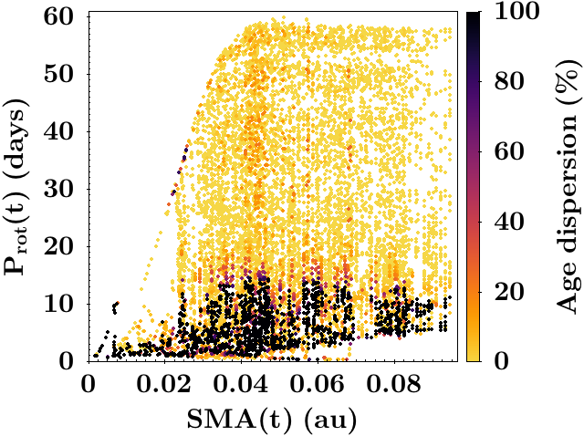
Figure 6: Same as Fig. 4, but for $\Delta\rm P_{\rm rot,\star}=0.1$ days.

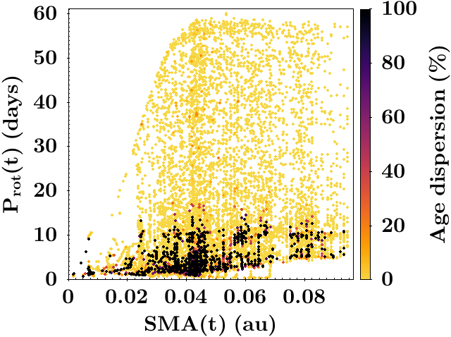
Figure 7: Same as Fig. 4, but for $\Delta\rm P_{\rm rot,\star}=0.01$ days.

Appendix C Tidal dissipation intensity and age estimation?

Table 6: Error on the estimation of the age provided by the gyrochronology analysis in the case of $|\rm\delta P|=0.5$. Here we consider a 0.7 $\rm M_{\odot}$ star around which orbits a 2 $\rm M_{jup}$ planet and for ¡$\mathcal{D}$¿= ¡$\mathcal{D}$¿_∗100.

Mass	$\rm P_{init}$	$\rm SMA_{init}$	$\rm Age_{50\%}$	$\Delta t_{50\%}$	$\rm P_{rot,50\%}$	$\rm P_{orb,50\%}$	$\rm P_{rot,isol.,50\%}$	$\rm Age_{gyro}$	$\rm Age_{gyro,isol.}$
($M_{\odot}$)	(days)	(au)	(Myr)	(Myr)	(days)	(days)	(days)	(Myr)	(Myr)
0.7	6.00	0.0258	164/624	40/80	4.16/7.72	–/–	8.25/11.86	84/256	288/549
0.7	7.00	0.0286	965/4155	140/1550	10.05/17.94	–/0.2630	15.59/36.71	409/1151	895/4133
0.7	8.00	0.0209	1655/1655	250/250	13.11/13.11	–/–	21.19/21.19	657/657	1549/1549
0.7	9.00	0.0226	3856/3856	1350/1350	18.46/18.46	0.2639/0.2633	34.86/34.86	1211/1211	3770/3770
0.7	10.40	0.0248	8707/8707	3400/3400	19.48/19.48	0.2642/0.2637	50.55/50.55	1333/1333	7319/7319

• We adopted a dissipation that is two orders of magnitude higher ¡$\mathcal{D}$¿_∗100 than the frequency-averaged tidal dissipation used in this article. The listed data are for ¡$\mathcal{D}$¿_∗100 (left) and ¡$\mathcal{D}$¿ (right) and in the case of $|\rm\delta P|=0.50$. We only show data that are in common between the two datasets.

Table 7: Same as Table 6, but for a dissipation two orders of magnitude lower ¡$\mathcal{D}$¿_/100.

Mass	$\rm P_{init}$	$\rm SMA_{init}$	$\rm Age_{50\%}$	$\Delta t_{50\%}$	$\rm P_{rot,50\%}$	$\rm P_{orb,50\%}$	$\rm P_{rot,isol.,50\%}$	$\rm Age_{gyro}$	$\rm Age_{gyro,isol.}$
($M_{\odot}$)	(days)	(au)	(Myr)	(Myr)	(days)	(days)	(days)	(Myr)	(Myr)
0.7	5.00	0.0229	3253/263	400/20	16.81/2.55	0.2644/–	32.98/7.88	1025/35	3414/265
0.7	6.00	0.0230	3854/884	550/40	17.57/4.97	0.2641/–	35.69/14.30	1109/116	3931/767
0.7	7.20	0.0194	225/225	20/20	2.87/2.87	–/–	9.87/9.87	44/44	396/396
0.7	8.00	0.0209	1755/1755	100/100	9.51/9.51	–/–	21.91/21.91	370/370	1645/1645
0.7	9.00	0.0226	3906/3906	550/550	17.95/17.95	–/–	35.08/35.08	1152/1152	3812/3812
0.7	10.40	0.0248	8707/8707	1500/1500	19.48/19.48	0.2642/0.2637	50.55/50.55	1333/1333	7319/7319

• The listed data are for ¡$\mathcal{D}$¿_/100 (left) and ¡$\mathcal{D}$¿ (right).

Tables 6 and 7 show that when the efficiency of the tidal dissipation is globally reduced (increased) by a factor of 100, the star-planet tidal interaction timescale globally decreases (increases) compared to the normal tidal dissipation efficiency.