Kramers-Kronig relations
beyond the optical approximation

Abstract

Kramers-Kronig relations are extended to dielectric functions $\varepsilon(q,\omega)$ that depend not only on the angular frequency $\omega$ but on the wave number $q$ as well. This implies extending the notion of causality commonly used in the theory of Kramers-Kronig relations to include the fact that signals cannot propagate faster than light in vacuo.
The results derived here also apply to general theories of isotropic linear response in which the response function depends on both the wave number and the frequency.

1 Introduction

The optical properties of materials, in other words, the response to spatially homogeneous electromagnetic fields, are usually described by the optical dielectric function (ODF), $\varepsilon(\omega)$, a complex function of the angular frequency $\omega$ of the Fourier components of the field [1], [2]. The refractive index, $n(\omega)$, and the extinction coefficient, $\kappa(\omega)$, are, respectively, the real and imaginary parts of the complex refractive index,

$$N(\omega)=\varepsilon^{1/2}(\omega)=n(\omega)+{\rm i}\kappa(\omega).$$ (1)

In principle, the optical functions $n(\omega)$ and $\kappa(\omega)$ can be measured by a combination of experimental techniques that operate over different frequency ranges. To assemble a consistent description of the optical functions of a material, covering the entire range of frequencies, results from various techniques have to be combined. The consistency of the resulting empirical functions can be examined by using Kramers-Kronig analysis [3].

The response of the material to spatially inhomogeneous electromagnetic fields is characterized by the dielectric function (DF), $\varepsilon({\bf q},\omega)$, a function of the wave vector ${\bf q}$ and the angular frequency. Knowledge of the DF allows the calculation of the stopping power of fast charged particles as the result of the force on the projectile acted by the electric field induced within the material by the projectile charge itself. In most practical cases the material is assumed to be homogeneous and isotropic, for which the dielectric function $\varepsilon(q,\omega)$ depends on only the wavenumber $q$. For such materials, a classical calculation [4] gives the stopping power as

$$S=\frac{(Z_{0}e)^{2}}{\pi v^{2}}\;{\rm Im}\int_{0}^{\infty}\omega\,{\rm d}\omega\int_{(\omega/v)^{2}}^{\infty}\frac{{\rm d}(q^{2})}{q^{2}}\left[\frac{-1}{\varepsilon^{\rm(L)}(q,\omega)}+\frac{c^{2}\beta^{2}q^{2}-\omega^{2}}{c^{2}q^{2}-\omega^{2}\,\varepsilon^{\rm(T)}(q,\omega)}\right].$$ (2)

where $\varepsilon^{\rm(L)}$ and $\varepsilon^{\rm(T)}$ are the longitudinal and transverse DFs, respectively. In the limit ${\bf q}\rightarrow 0$, both DFs reduce to the ODF,

$$\lim_{{\bf q}\rightarrow 0}\varepsilon^{\rm(L)}({\bf q},\omega)=\lim_{{\bf q}\rightarrow 0}\varepsilon^{\rm(T)}({\bf q},\omega)=\varepsilon(\omega).$$ (3)

Practical calculations of inelastic collisions of charged particles in materials are frequently based on optical-data models [5] that combine an empirical ODF with suitable extension algorithms to produce a model of the full DF, i. e. of the function $\varepsilon(q,\omega)$ for $q>0$. The most elaborate extension algorithms rely on the DFs of the electron gas derived by Lindhard [4] and Mermin [6]. Optical-data models have often been employed in calculations of inelastic mean free paths and stopping powers of electrons in solids (see e. g. [7], [8], [9] and [10]). The quality of an optical-data model is determined by the consistency of the adopted ODF and by the adequacy of the extension algorithms.

Kramers-Kronig relations are restrictions [1], [2] that apply to the optical dielectric function $\varepsilon(\omega)$ —or to the electric susceptibility $\chi(\omega)\,$— of a linear material medium in the optical approximation, when the dependence on the wave vector $\mathbf{q}$ is neglected. Such relations follow from two rather general assumptions, namely (1) causality in time and (2) a certain behaviour of the ODF at high-$\omega$. In other words, the derivation assumes that the applied fields do not vary appreciably in space.

The interest of Kramers-Kronig relations is twofold: first, they provide a useful tool to analyze the consistency of empirical ODFs and, second, they are also a quality test that has to be passed by any acceptable expression of $\varepsilon(\omega)$ derived from whichever microscopic model [4].

To study the implications of causality for fields varying in both time and space it is necessary to account for the effect of retardation, i. e. for the finite velocity of propagation of the fields. The goal of the present work is to derive a generalization of the Kramers-Kronig relations for the entire DF, that is, for $q\neq 0$. Aside from its fundamental interest, this generalization can be employed to exhibit the consistency, or the lack of it, of extension algorithms adopted in optical-data models.

The assumption of causality means that

The polarization vector $\mathbf{P}(\mathbf{x},t)$ only depends on the values of the electric field $\mathbf{E}(\mathbf{x},t^{\prime})$ at the same place and at previous times, $t^{\prime}\leq t$.

If a linear isotropic medium responds to an applied harmonic, or monochromatic, electric field $\mathbf{E}(\mathbf{x},\omega)\,e^{-i\omega t}$ by adquiring a polarization $\mathbf{P}(\mathbf{x},\omega)\,e^{-i\omega t}$, both magnitudes are proportional

$$\mathbf{P}(\mathbf{x},\omega)=\chi(\omega)\,\mathbf{E}(\mathbf{x},\omega)$$ (4)

with the susceptibility $\chi(\omega)$ depending on the frequency. Linearity also implies that the response to a superposition of harmonic fields $\quad\displaystyle{\mathbf{E}(\mathbf{x},t)=\frac{1}{\sqrt{2\pi}}\,\int_{\mathbb{R}}{\rm d}\omega\,e^{-i\omega t}\,\mathbf{E}(\mathbf{x},\omega)}\,$ is the superposition of responses

$$\mathbf{P}(\mathbf{x},t)=\frac{1}{\sqrt{2\pi}}\,\int_{\mathbb{R}}{\rm d}\omega\,e^{-i\omega t}\,\chi(\omega)\,\mathbf{E}(\mathbf{x},\omega)$$

and, by the convolution theorem [11],

$$\mathbf{P}(\mathbf{x},t)=\frac{1}{\sqrt{2\pi}}\,\int_{\mathbf{R}}{\rm d}t^{\prime}\,\tilde{\chi}(t-t^{\prime})\,\mathbf{E}(\mathbf{x},t^{\prime})\,,\qquad{\rm with}\quad\tilde{\chi}(t)=\frac{1}{\sqrt{2\pi}}\,\int_{\mathbb{R}}{\rm d}\omega\,e^{-i\omega t}\,\chi(\omega)$$ (5)

Causality means that the effect $\mathbf{P}(\mathbf{x},t)$ cannot depend on the causes $\mathbf{E}(\mathbf{x},t^{\prime})$ at later times, which implies that

$$\tilde{\chi}(t-t^{\prime})=0\qquad{\rm for}\qquad t^{\prime}>t$$

We shall refer to this as local causality (L-causality), to distinguish it from other causality conditions that we shall introduce below.

Often the optical approximation does not suffice to account for the experimental results. The present view of a material medium as linearly reacting to the excitation produced by the electromagnetic field is a macroscopic description which can be modeled as the linear approximation to the collective response of the elementary charges contained in the medium. The different microscopic models [4] basically consist of analyzing the electromagnetic forces exerted by the field on the elementary charges or, equivalently, the energy and momentum exchange among field and charges. For a plane electromagnetic wave, energy and momentum are exchanged in multiples of $\hbar\omega$ and $\hbar\mathbf{q}$, respectively. In some instances —for “small” $|\mathbf{q}|$— the optical approximation $\varepsilon(\omega)$ yields a fairly good description of experimental results, but for higher values of $|\mathbf{q}|$, the effect of momentum exchange becomes important and it is necessary to consider the dependence of the dielectric function on the wave vector as well.

If we go beyond the optical approximation, the dielectric function $\varepsilon(\mathbf{q},\omega)$ depends on the frequency and on the wave vector of the electric field and the same holds for electrical susceptibility,

$$\chi(\mathbf{q},\omega)=\frac{\varepsilon(\mathbf{q},\omega)-1}{4\pi}\,.$$

In this case the causality condition will be more complex than for L-causality. Indeed, an analogous to the expression (4) for the polarization obtained as a linear isotropic response to a plane monochromatic wave is

$$\mathbf{P}(\mathbf{q},\omega)\,e^{i(\mathbf{q}\cdot\mathbf{x}-\omega t)}=\chi(\mathbf{q},\omega)\,\mathbf{E}(\mathbf{q},\omega)\,e^{i(\mathbf{q}\cdot\mathbf{x}-\omega t)}$$ (6)

As before, linearity implies that the response to a superposition of plane monochromatic electromagnetic waves,

$$\,\mathbf{E}(\mathbf{x},t)=\frac{1}{(2\pi)^{2}}\,\int_{\mathbb{R}^{4}}{\rm d}\mathbf{q}\,{\rm d}\omega\,\mathbf{E}(\mathbf{q},\omega)\,e^{i(\mathbf{q}\cdot\mathbf{x}-\omega t)}\,,$$

is given by

$$\,\mathbf{P}(\mathbf{x},t)=\frac{1}{(2\pi)^{2}}\,\int_{\mathbb{R}^{4}}{\rm d}\mathbf{q}\,{\rm d}\omega\,\chi(\mathbf{q},\omega)\mathbf{E}(\mathbf{q},\omega)\,e^{i(\mathbf{q}\cdot\mathbf{x}-\omega t)}$$

and, by the convolution theorem for Fourier transforms [11],

$$\mathbf{P}(\mathbf{x},t)=(2\pi)^{-2}\,\int_{\mathbf{R}^{4}}{\rm d}\mathbf{y}\,{\rm d}t^{\prime}\,\tilde{\chi}(\mathbf{x}-\mathbf{y},t-t^{\prime})\,\mathbf{E}(\mathbf{y},t^{\prime})\,,$$ (7)

where

$$\tilde{\chi}(\mathbf{x},t)=(2\pi)^{-2}\,\int_{\mathbb{R}^{4}}{\rm d}\mathbf{q}\,{\rm d}\omega\,\chi(\mathbf{q},\omega)\,e^{i(\mathbf{q}\cdot\mathbf{x}-\omega t)}$$ (8)

is the susceptibility function in spacetime variables. In what follows we shall use the same letter to indicate a physical magnitude, either as a function in wave vector-frequency variables $(\mathbf{q},\omega)$ or in spacetime variables $(\mathbf{x},t)$. In this second case the symbol is indicated with the diacritic “$\;\tilde{}\;$”.

Notice that equation (7) is invariant under spacetime translations, i. e. replacing the electric field by $\mathbf{E}^{\prime}(\mathbf{y},t^{\prime})=\mathbf{E}(\mathbf{y}-\mathbf{x}_{0},t^{\prime}-t_{0})\,$ results in a new polarization $\mathbf{P}^{\prime}(\mathbf{y},t^{\prime})=\mathbf{P}(\mathbf{y}-\mathbf{x}_{0},t^{\prime}-t_{0})\,$. Thus the convolution relation (7) implies that the material medium is homogeneous in space and time, whence it follows that assuming the relation (6) actually amounts to assuming homogeneity.

In turn the susceptibility in wave vector-frequency space is the inverse Fourier transform

$$\chi(\mathbf{q},\omega)=(2\pi)^{-2}\,\int_{\mathbb{R}^{4}}{\rm d}\mathbf{x}\,{\rm d}t\,\tilde{\chi}(\mathbf{x},t)\,e^{i(\omega t-\mathbf{q}\cdot\mathbf{x})}$$ (9)

In the present work we shall restrict ourselves to isotropic media, i. e. such that $\,\tilde{\chi}(\mathbf{x},t)\ =\tilde{\chi}(r,t)\,$ only depends on the distance $\,r=|\mathbf{x}|\,$ and not on the direction of $\,\mathbf{x}\,$, and therefore $\,\chi(\mathbf{q},\omega)\ =\chi(q,\omega)\,$.

The expression (7) means that the polarization at point $\mathbf{x}$ at instant $t$ is the “effect” of infinitely many “causes”, namely the values of the electric field at every place $\mathbf{y}$ and every instant $t^{\prime}$. We then expect that the influence of $\mathbf{E}(\mathbf{y},t^{\prime})$ on $\mathbf{P}(\mathbf{x},t)$ does not travel faster than light $c$ in vacuum. Expressed in terms of spacetime variables this causality condition reads

The polarization $\mathbf{P}(\mathbf{x},t)$ only depends on the values of the electric field $\mathbf{E}(\mathbf{y},t^{\prime})$ in the absolute past

$$0\leq|\mathbf{x}-\mathbf{y}|\leq(t-t^{\prime})c\,,$$ (10)

i. e. the event $(\mathbf{y},t^{\prime})$ is in the past light cone with vertex $(\mathbf{x},t)$.

Hence, the signals connecting the causes $\mathbf{E}(\mathbf{y},t^{\prime})$ with the effect $\mathbf{P}(\mathbf{x},t)$ may not travel faster than light in vacuum. We shall thus refer to the above condition as finite speed causality (FS-causality) to distinguish it from the standard Newtonian causality (N-causality), which might involve signals propagating as fast as necessary so as to permit an event at $t$ to be influenced by any event at $t^{\prime}\leq t$ no matter what the distance separating both.

Notice that FS-causality includes L-causality as a particular case. In light of equation (10), FS-causality amounts to the following constraint on the response function

$$c(t-t^{\prime})<|\mathbf{x}-\mathbf{y}|\qquad\Rightarrow\qquad\tilde{\chi}(\mathbf{x}-\mathbf{y},t-t^{\prime})=0\,.$$ (11)

and therefore $\qquad t<0\quad\Rightarrow\quad tc<|\mathbf{x}|\quad\Rightarrow\quad\tilde{\chi}(t)=\tilde{\chi}(\mathbf{x},t)=0\,$. This is due to the fact that in the optical approximation the convolution formula (5) involves only one space point, hence it does not imply the propagation at a distance of any signal.

In the same way as the Kramers-Kronig relations, our approach can be also applied in the context of any theory of linear response [12] based on a triple, Input-Output-Response function (I-O-RF), that are connected by a relation of the sort (7) or (6), where the triple is Electric field-Polarization-Susceptibility. A similar connection is found in scattering processes, e. g. [13] and [14], where the triple consists of Incoming wave, Scattered wave, and $S$-matrix.

The condition that we have called FS-causality has been also explicitly invoked elsewhere, see refs. [15] to [22] to quote a few but, curiously, Toll’s paper [15] obviates the spatially dispersive case, in which the response function should also depend on the wave vector $\mathbf{q}\,$.

Leontovich’s work [16] is the most accomplished previous attempt to extend the Kramers-Kronig relations to media with spatial dispersion. He considers the connection of electric field (I) and current density (O) through conductivity $\sigma(q,\omega)$ (RF) and assumes that the latter is the same in all inertial reference frames. Yet his reasoning seems restricted to fields that depend only on one space coordinate. Moreover, the assumption that $\sigma$ is a Lorentz scalar is questioned by some authors, [17] to [20], who obtain exactly the same generalization of Kramers-Kronig relations. This suggests that Lorentz invariance or covariance is not essential for Leontovich’s generalization and we shall here derive it on the basis of relativistic causality (FS-causality), which is a more generic assumption.

In what follows we shall find out the implications of FS-causality on the dielectric function $\varepsilon(q,\omega)$ —or alternatively, the electric susceptibility $\chi(q,\omega)\,$— and we will restrict our considerations to isotropic media. We shall proceed in much the same way as standard textbooks [1] derive Kramers-Kronig relations. In Section 2 we prove that FS-causality implies that susceptibility is a doubly analytic function in some region in $\mathbb{C}^{2}$, the complex planes spanned by complex $q$ and $\omega$. In Section 3 we derive a generalization of Kramers-Kronig relations suitable for FS-causality and compare it with previous results [16]. Finally in Section 4 several dielectric functions commonly used in the literature are examined to check whether they satisfy the FS-causality condition. Although most results in the present paper are stated for the electric susceptibility $\chi$, they also hold for the dielectric function.

2 Consequences of finite speed causality on the susceptibility function

As mentioned above, FS-causality amounts to equation (11), that is

$$\tilde{\chi}(\mathbf{x},t)\propto\Theta(ct-r)\,,$$ (12)

where $r=|\mathbf{x}|$ and $\Theta\,$ is the Heaviside unit step function. This implies that the susceptibility function in the wave vector-frequency space is

$$\chi(\mathbf{q},\omega)=\frac{i}{2\pi\,q}\,\int_{0}^{\infty}{\rm d}t\,\int_{-ct}^{ct}{\rm d}r\,r\,\tilde{\chi}(r,t)\,e^{i(\omega t-qr)}\,,$$

where we have integrated over the angular spherical coordinates and have introduced

$$\tilde{\chi}(-r,t)=\tilde{\chi}(r,t)\,,\qquad\qquad r>0$$ (13)

as an extension of the susceptibility to negative values of $\,r\,$ —moreover, we restrict to the isotropic case. Thus $\,\chi(\mathbf{q},\omega)\,$ depends only on $\,\omega\,$ and $\,q=|\mathbf{q}|\,$ as expected and, writing $\,\chi(q,\omega)\,$ to stress this fact, we have that

$$q\,\chi(q,\omega)=\frac{i}{2\pi}\,\int_{0}^{\infty}{\rm d}t\,\int_{-ct}^{ct}{\rm d}r\,e^{i(\omega t-qr)}\,r\,\tilde{\chi}(r,t)\,.$$ (14)

It can be easily shown that $\,\chi(q,\omega)\,$ is an even function of $\,q\,$.

We now introduce the “light-cone” coordinates and frequencies

$$u^{\pm}=\frac{1}{2}\,(ct\mp r)\,,\qquad\qquad k_{\pm}=\frac{\omega}{c}\pm q$$ (15)

and the inverse relations

$$ct=u^{+}+u^{-}\,,\qquad r=u^{-}-u^{+}\,,\qquad\frac{\omega}{c}=\frac{k_{+}+k_{-}}{2}\,,\qquad q=\frac{k_{+}-k_{-}}{2}\,.$$ (16)

In turn the “volume elements” transform as $\;c\,{\rm d}t\,{\rm d}r=2\,{\rm d}u^{+}\,{\rm d}u^{-}\,$, and $\;2\,{\rm d}q\,{\rm d}\omega=c\,{\rm d}k_{+}\,{\rm d}k_{-}$ and the integration domain $\,\mathcal{D}=\left\{(r,t)\,,\;|r|\leq ct\right\}\,$ becomes the first quadrant $\,\mathcal{D}^{\prime}=[0,\infty)\times[0,\infty)\,$. Using this and the fact that $\,\omega t-qr=k_{+}u^{+}+k_{-}u^{-}\,$, the relation (14) can be written as

$$(k_{+}-k_{-})\,\xi(k_{+},k_{-})=-\frac{2\,i}{\pi c}\,\int_{0}^{\infty}{\rm d}u^{+}\,e^{-(0-ik_{+})u^{+}}\,\int_{0}^{\infty}{\rm d}u^{-}\,e^{-(0-ik_{-})u^{-}}\,(u^{+}-u^{-})\,\tilde{\xi}(u^{+},u^{-})\,,$$ (17)

where, for the sake of future clarity, we write

$$\xi(k_{+},k_{-}):=\chi(q,\omega)\qquad{\rm and}\qquad\tilde{\xi}(u^{+},u^{-}):=\tilde{\chi}(r,t)\,,$$ (18)

that is we use a different symbol for the susceptibility depending on whether the independent variables are $(q,\omega)$ or $(k_{+},k_{-})\,$. The expressions $\,0-i\,k_{\pm}\,$ in the exponents mean that the integrals are to be calculated for $\,\delta-i\,k_{\pm}\,$ and then take the limit for $\delta\rightarrow 0^{+}\,$.

The above relations can be read as a double Laplace transform. Indeed, defining

$$G(u^{+},u^{-}):=-\frac{2\,i}{\pi c}\,(u^{+}-u^{-})\,\tilde{\xi}(u^{+},u^{-})\,,\qquad\qquad h(k_{+},k_{-}):=(k_{+}-k_{-})\,\xi(k_{+},k_{-})\,,$$ (19)

and introducing

$$g(s_{+},s_{-})=\int_{\mathbb{R}^{+\,2}}{\rm d}u^{+}\,{\rm d}u^{-}\,G(u^{+},u^{-})\,e^{-s_{+}u^{+}-s_{-}u^{-}}\,,$$ (20)

we have that

$$h(k_{+},k_{-})=g(0-ik_{+},0-ik_{-})$$ (21)

Invoking now a well known property of the Laplace transform [11], it results that, if

$$\int_{\mathbb{R}^{+\,2}}{\rm d}u^{+}\,{\rm d}u^{-}\,G(u^{+},u^{-})\,e^{-a_{+}u^{+}-a_{-}u^{-}}<\infty\,$$ (22)

for some real numbers $\,a_{\pm}\,$, then $\,g(s_{+},s_{-})\,$ is analytic in the product of half-planes $\,{\mathbb{R}}{\rm e}\,\left(s_{\pm}\right)>a_{\pm}\,$ which, recalling (21), means that

$$h(k_{+},k_{-})\quad\mbox{is doubly analytic if}\quad{\mathbb{I}}{\rm m}\,\left(k_{+}\right)>a_{+}\quad{\rm and}\quad{\mathbb{I}}{\rm m}\,\left(k_{-}\right)>a_{-}$$ (23)

We shall refer to the variables $k_{\pm}$ as light cone frequencies because, similarly as $\mathbf{q}$ and $\omega$ are the Fourier conjugates of $\mathbf{r}$ and $t$, $\,k_{\pm}\,$ are the Fourier conjugates of the light cone variables $\,u^{\pm}\,$. Now we need to make a detour to establish some preliminary results that will be helpful in proving the existence of the double Laplace transform $\,g(s_{+},s_{-})\,$ for ${\mathbb{R}}{\rm e}\,(s_{\pm})>0\,$.

2.1 Symmetries

The functions $\,\tilde{\xi}(u^{+},u^{-})\,$ and $\,\xi(k_{+},k_{-})\,$ present some obvious symmetries. In terms of the light cone variables variables (15), the extension (13) introduced above implies that

$$\tilde{\xi}(u^{+},u^{-})=\tilde{\xi}(u^{-},u^{+})\,,$$ (24)

therefore $\tilde{\xi}(u^{+},u^{-})\,$ is invariant if we swap the variables. Using light cone variables, the FS-causality condition (12) reads $\,\tilde{\xi}(u^{+},u^{-})\propto\Theta(u^{+})\,$ which, combined with (24) implies that

$$\tilde{\xi}(u^{+},u^{-})\propto\Theta(u^{+})\,\Theta(u^{-})$$ (25)

and therefore $\,\tilde{\xi}(u^{+},u^{-})\,$ vanishes outside the first quadrant, $\,[0,\infty)\times[0,\infty)\,$.

By direct inspection of equation (17), we easily see that the symmetry (24) also holds for the Fourier transform

$$\xi(k_{+},k_{-})=\xi(k_{-},k_{+})$$ (26)

Furthermore, since $\,\tilde{\xi}(u^{+},u^{-})\,$ must be real for real $u^{\pm}\,$, the complex conjugate of the relation (17) leads to

$$\xi(-k_{+},-k_{-})=\xi^{\ast}(k_{+},k_{-})\,,$$ (27)

for real $\,k_{\pm}\,$, where the superscript ${\,}^{\ast}\,$ means “complex conjugate”. In terms of $\,h(k_{+},k_{-})\,$ the relations (26) and (27) become

$$h(k_{-},k_{+})=-h(k_{+},k_{-})\qquad{\rm and}\qquad h(-k_{+},-k_{-})=-h^{\ast}(k_{+},k_{-})$$ (28)

(the second relation is meant for real values of the variables).

2.2 The function $h(k_{+},k_{-})\,$ at high frequencies

In order to determine the asymptotic behavior of $g(s_{+},s_{-})$ for large values of $\,s_{\pm}\,$ we use the following theorem which is proved in the Appendix.

Theorem 1

Let $\,g(s_{+},s_{-})\,$ be the double Laplace integral (20), assume that $\,G(u^{+},u^{-})\,$ has continuous partial derivatives $\,G^{(l,j)}(u^{+},u^{-})=\partial_{+}^{l}\partial_{-}^{j}G(u^{+},u^{-})\,$ up to the $N$-th order (i. e. $l+j\leq N$) and that there exist $\,a_{\pm}\in\mathbb{R}\,$ such that

$$\,\int_{\mathbb{R}^{+2}}{\rm d}u^{+}\,{\rm d}u^{-}\,G^{(l,j)}(u^{+},u^{-})e^{-a_{+}u^{+}-a_{-}u^{-}}<\infty\,,\qquad\quad l+j\leq N\,,$$

then

$$g(\lambda s_{+},\lambda s_{-})=\sum_{0\leq l+j\leq N-1}\frac{G^{(l,j)}(0^{+},0^{+})}{\lambda^{l+j+2}s_{+}^{l+1}s_{-}^{j+1}}+o(\lambda^{-N-1})\,,\qquad\qquad\forall\lambda\in\mathbb{R}^{+}\,.$$

We then say that the asymptotic behavior of $g(s_{+},s_{-})$ up to order $N-1$ is

$$g(s_{+},s_{-})\sim\sum_{l+j=0}^{N-1}\,\frac{G^{(l,j)}(0^{+},0^{+})}{s_{+}^{l+1}\,s_{-}^{j+1}}\qquad{\rm when}\qquad s_{\pm}\rightarrow\infty\,,\qquad\left|{\rm arg}(s_{\pm}-a_{\pm})\right|<\frac{\pi}{2}$$ (29)

where $\,G^{(l,j)}(0^{+},0^{+})\,$ are the lateral partial derivatives of $G$.

In order to derive the coefficients of the asymptotic expansion we differentiate (19) and, on iterating the Leibniz rule, we obtain that

$$G^{(0,0)}(0^{+},0^{+})=0\,,\qquad\qquad G^{(1,0)}(0^{+},0^{+})=-G^{(0,1)}(0^{+},0^{+})=-\frac{2\,i}{\pi c}\,\tilde{\xi}(0^{+},0^{+})\qquad{\rm and}$$

$$G^{(l,j)}(0^{+},0^{+})=-\frac{2i}{\pi c}\,\left[l\,\tilde{\xi}^{(l-1,j)}(0^{+},0^{+})-j\,\tilde{\xi}^{(l,j-1)}(0^{+},0^{+})\right]$$ (30)

Thus the lowest order in the asymptotic expansion (29) corresponds to $N=2$ and yields

$$g(s_{+},s_{-})\sim\frac{2\,i\,\tilde{\xi}(0^{+},0^{+})}{\pi c}\,\frac{s_{+}-s_{-}}{s_{+}^{2}\,s_{-}^{2}}$$

and, using (19) and (21), we have that

$$h(k_{+},k_{-})\sim\frac{2\,\tilde{\xi}(0^{+},0^{+})}{\pi c}\,\frac{k_{+}-k_{-}}{k_{+}^{2}\,k_{-}^{2}}\qquad{\rm or}\qquad\chi(q,\omega)\sim\frac{2c^{3}\,\tilde{\chi}(0,0^{+})}{\pi(c^{2}q^{2}-\omega^{2})^{2}}\,,$$ (31)

provided that the partial derivatives $\,G^{(l,j)}(u^{+},u^{-})=\partial_{+}^{l}\partial_{-}^{j}G(u^{+},u^{-})\,$ are continuous for $l,\,j\leq 2\,$ and $u^{\pm}>0\,$, which amounts to the continuity of $\tilde{\chi}^{(l,j)}(r,t)$ for $l,\,j\leq 2\,$in the region $ct>|r|\,$.

$\tilde{\xi}(u^{+},u^{-})\,$ vanishes when either $u^{+}$ or $u^{-}$ are negative and one might require that it does not start abruptly, in other words, the function is continuous at the boundary

$$\tilde{\xi}(u^{+},0)=\tilde{\xi}(0,u^{-})=0\,.$$

Therefore $\quad\tilde{\xi}^{(l,0)}(0,0)=\tilde{\xi}^{(0,j)}(0,0)=0\,$ which, substituted in (30) implies that

$$G^{(l,0)}(0,0)=G^{(0,j)}(0,0)=0$$ (32)

and also

$$G^{(l,1)}(0^{+},0^{+})=-i\,\frac{2l}{\pi c}\,\tilde{\xi}^{(l-1,1)}(0^{+},0^{+})\,,\qquad G^{(1,j)}(0^{+},0^{+})=i\frac{2j}{\pi c}\,\tilde{\xi}^{(1,j-1)}(0^{+},0^{+})$$ (33)

Hence the lowest non-vanishing coefficients in the expansion (29) are

$$G^{(2,1)}(0^{+},0^{+})=-G^{(1,2)}(0^{+},0^{+})=-i\,\frac{4}{\pi c}\,\tilde{\xi}^{(1,1)}(0^{+},0^{+})$$

Including these, the lowest order in the asymptotic expansion (29) is

$$g(s_{+},s_{-})\sim-i\frac{4}{\pi c}\,\tilde{\xi}^{(1,1)}(0^{+},0^{+})\,\frac{s_{-}-s_{+}}{s_{+}^{3}s^{3}_{-}}$$

Then, including (21), we have that

$$h(k_{+},k_{-})\sim-\frac{4\,(k_{+}-k_{-})}{\pi\,c\,k_{+}^{3}k_{-}^{3}}\,\tilde{\xi}^{(1,1)}(0^{+},0^{+})$$ (34)

and therefore

$$\xi(k_{+},k_{-})\sim-\frac{4}{\pi\,c\,k_{+}^{3}k_{-}^{3}}\,\tilde{\xi}^{(1,1)}(0^{+},0^{+})\qquad{\rm or}\qquad\chi(q,\omega)\sim-\frac{4c^{3}}{\pi\,(\omega^{2}-c^{2}q^{2})^{3}}\,\left(\partial_{t}^{2}\tilde{\chi}-c^{2}\partial_{r}^{2}\tilde{\chi}\right)_{(0^{+},0)}$$ (35)

where $\,(0^{+},0)\,$ means the limit for $t\rightarrow 0^{+}\,$, when $\,|r|<ct\,$.

2.3 The existence of the Laplace transform $g(s_{+},s_{-})$

For a non-conductor it is expected that a constant uniform electric field produces a finite polarization. If we now put $\mathbf{E}(\mathbf{x},t)=\mathbf{E}\,$, a constant, in equation (7), we have that the polarization is constant

$$\mathbf{P}=\frac{1}{\pi}\,\mathbf{E}\,\int_{0}^{\infty}{\rm d}t\,\int_{0<r<ct}{\rm d}r\,r^{2}\tilde{\chi}(t,r)=\frac{1}{\pi c}\,\mathbf{E}\,\int_{\mathbf{R}^{+}}{\rm d}u^{+}\,\int_{\mathbf{R}^{+}}{\rm d}u^{-}\,(u^{+}-u^{-})^{2}\,\tilde{\xi}(u^{+},u^{-})\,,$$

which is finite if, and only if,

$$\int_{\mathbf{R}^{+\,2}}{\rm d}u^{+}\,{\rm d}u^{-}\,\tilde{\xi}(u^{+},u^{-})\,(u^{+}-u^{-})^{2}<\infty$$ (36)

where the definition (18) has been included.

Thus the function

$$F(u^{+},u^{-})=\tilde{\xi}(u^{+},u^{-})\,(u^{+}-u^{-})^{2}=G(u^{+},u^{-})\,(u^{+}-u^{-})$$ (37)

must be summable in $\mathbb{R}^{+\,2}$, which implies both the existence of the double Laplace transform,

$$\,f(s_{+},s_{-})=\int_{\mathbf{R}^{+\,2}}{\rm d}u^{+}\,{\rm d}u^{-}\,F(u^{+},u^{-})\,e^{-(s_{+}u^{+}+s_{-}u^{-})}\,$$

and its analyticity in the product of complex half-planes ${\mathbb{R}}{\rm e}\,(s_{\pm})>0$.

Reasoning similarly as in section 2.2, we arrive at the asymptotic expansion

$$f(s_{+},s_{-})\sim\sum_{l,j}F^{(l,j)}(0^{+},0^{+})\,\frac{1}{s_{+}^{l+1}\,s_{-}^{j+1}}\,,\qquad\mbox{for large }\,s_{\pm}$$

and, applying a similar reasoning as there to the function $\,F(u^{+},u^{-})\,$ instead of $\,G(u^{+},u^{-})\,$, we have that

$$F^{(l,j)}(0^{+},0^{+})=-\frac{2i}{\pi c}\,\left[l(l-1)\,\tilde{\xi}^{(l-2,j)}(0^{+},0^{+})+j(j-1)\,\tilde{\xi}^{(l,j-2)}(0^{+},0^{+})-2\,j\,l\,\tilde{\xi}^{(l-1,j-1)}(0^{+},0^{+})\right]$$

and the lowest non-vanishing derivative is

$$F^{(1,1)}(0^{+},0^{+})=\frac{4i}{\pi c}\,\tilde{\xi}(0^{+},0^{+})$$

Then the asymptotic expansion at the lowest order reads

$$f(s_{+},s_{-})\sim\,\frac{4i}{\pi\,c\,s_{+}^{2}s_{-}^{2}}\,\tilde{\xi}(0^{+},0^{+})$$ (38)

and $\,f(s_{+},s_{-})\rightarrow 0\,$ for large $\,s_{+},\,s_{-}\,$.

On the other hand the Laplace transform of the relation (37) implies that

$$f(s_{+},s_{-})=-\left(\partial_{+}-\partial_{-}\right)\,g(s_{+},s_{-})\,$$ (39)

(here $\partial_{\pm}$ means the partial derivative with respect to $s_{\pm}\,$) which on integration yields

$$g(s_{+},s_{-})=i\,\int_{0}^{\infty}{\rm d}\sigma\,f(s_{+}+i\sigma,s_{-}-i\sigma)$$ (40)

where the asymptotic behaviour of $\,f(s_{+},s_{-})\,$ has been used. Indeed,

$$\left(\partial_{+}-\partial_{-}\right)\,g(s_{+},s_{-})=i\,\int_{0}^{\infty}{\rm d}\sigma\,\left[\partial_{+}f(s_{+}+i\sigma,s_{-}-i\sigma)-\partial_{-}f(s_{+}+i\sigma,s_{-}-i\sigma)\right]$$

$$\qquad=\int_{0}^{\infty}{\rm d}\sigma\,\partial_{\sigma}f(s_{+}+i\sigma,s_{-}-i\sigma)=\left[f(s_{+}+i\sigma,s_{-}-i\sigma)\right]_{0}^{\infty}=-f(s_{+},s_{-})$$

Whenever $\,{\mathbb{R}}{\rm e}\,(s_{\pm})>0\,$ the value $\,f(s_{+}+i\sigma,s_{-}-i\sigma)\,$ is well defined and, due to its asymptotic behaviour, the integral in (40) converges. Therefore $\,g(s_{+},s_{-})\,$ exists and is doubly analytic in the region $\,{\mathbb{R}}{\rm e}\,(s_{\pm})>0\,$.

As a consequence the function $h(k_{+},k_{-})=g(0-ik_{+},0-ik_{-})$ is analytic in the region $\,{\mathbb{I}}{\rm m}\,(k_{\pm})>0\,$ which in terms of the frequency $\omega$ and wave vector $q$ implies that

$$q\,\chi(q,\omega)\quad\mbox{is doubly analytic in}\quad c\,\left|{\mathbb{I}}{\rm m}\,(q)\right|<{\mathbb{I}}{\rm m}\,(\omega)$$ (41)

or, equivalently,

$$\mbox{all singularities of}\quad q\,\chi(q,\omega)\quad\mbox{lie in the region}\quad{\mathbb{I}}{\rm m}\,(\omega)\leq c\,\left|{\mathbb{I}}{\rm m}\,(q)\right|$$ (42)

These two equivalent statements are the consequence of FS-causality for a non-conductor.

2.4 The absence of spatial dispersion.

If there is no spatial dispersion, the susceptibility function and its Fourier transform are

$$\chi(q,\omega)=\chi(\omega)\qquad\qquad{\rm and}\qquad\qquad\tilde{\chi}(\mathbf{x},t)=\tilde{\chi}(t)\,\delta(\mathbf{x})$$ (43)

respectively. When $\tilde{\chi}(\mathbf{x},t)$ factorizes like this, the L-causality and FS-causality conditions are equivalent. Indeed, in terms of spacetime variables:

L-causality $\Rightarrow$ FS-causality:

If $t<|\mathbf{x}|/c\,$, then either $|\mathbf{x}|\neq 0\,$ and $\tilde{\chi}(\mathbf{x},t)=0$ due to the $\delta$-function, or $|\mathbf{x}|=0\,$ and $\tilde{\chi}(t)=0$ too, due to to L-causality. Then in any case $\,\tilde{\chi}(\mathbf{x},t)=0\,$.

FS-causality $\Rightarrow$ L-causality:

If $t<0$, then $t<|\mathbf{x}|/c\,$, for any $\mathbf{x}\,$ and FS-causality implies that $\,\tilde{\chi}(\mathbf{x},t)=0\,$ for any $\mathbf{x}$  which, including (43), amounts to $\tilde{\chi}(t)=0$.

We might similarly reason in terms of the Fourier space frequencies as well:

• L-causality means that all singularities of the dielectric function $\chi(q,\omega)=\chi(\omega)$ lie in the region ${\mathbb{I}}{\rm m}\,(\omega)\leq 0$, that is ${\mathbb{I}}{\rm m}\,(\omega)\leq c\,|{\mathbb{I}}{\rm m}\,(q)|\,$, for all $q$, which amount to FS-causality, and conversely

• FS-causality implies that all singularities of $\chi(q,\omega)$ lie in the region ${\mathbb{I}}{\rm m}\,(\omega)\leq c\,|{\mathbb{I}}{\rm m}\,(q)|\,$ and, in particular, as $\chi(\omega)=\chi(q=0,\omega)$, all singularities of $\chi(\omega)$ lie in ${\mathbb{I}}{\rm m}\,(\omega)\leq 0\,$, which amounts to L-causality.

As for the asymtotic behavior, substituting (43) in (19), we have that

$$G(u^{+},u^{-})=-\frac{4\,i}{c\,\sqrt{2\pi}}\,\tilde{\chi}\left(\frac{u^{+}+u^{-}}{c}\right)\,\delta^{\prime}(u^{-}-u^{+})\,.$$

As it contains the derivative of a $\delta$-function, it is not a continuous function at the points $\,u^{+}=u^{-}\,$ in the quadrant $\mathbb{R}^{+}\times\mathbb{R}^{+}\,$, Theorem 1 does not apply and therefore $\chi(\omega)$ may not present the asymptotic behavior (35).

3 A generalization of Kramers-Kronig relations

In the optical approximation Kramers-Kronig relations connect the real and imaginary parts of electric susceptibility $\tilde{\chi}(\omega)$ in such a way that knowledge of one for all real values of $\omega$ determines the other: they are Hilbert transforms of each other [24]. These relations follow from: (i) the analyticity of $\chi(\omega)$ in the upper complex half-plane ${\mathbb{I}}{\rm m}\,(\omega)>0\,$ combined with (ii) a suitable asymptotic behavior for large $|\omega|\,$.

Beyond the optical approximation and assuming FS-causality we have that $h(k_{+},k_{-})=2q\,\chi(q,\omega)\,$ is analytic in the product of half-planes $\,{\mathbb{I}}{\rm m}\,(k_{\pm})>0\,$. We shall now proceed similarly as in the derivation of Kramers-Kronig relations [1] and consider the path $\mathcal{C}$ in the $\,k_{+}\,$ complex plane as depicted in Figure 1.

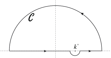
Figure 1: The integration path in the complex plane $k_{+}$

If $\,{\mathbb{I}}{\rm m}\,(k_{-})>0\,$, $h(k_{+},k_{-})$ is analytic in the half-plane ${\mathbb{I}}{\rm m}\,(k_{+})>0\,$ and Cauchy’s theorem [25] implies that

$$h(k_{+},k_{-})=\frac{1}{2\pi i}\,\oint_{\mathcal{C}}{\rm d}k^{\prime}\,\frac{h(k^{\prime},k_{-})}{k^{\prime}-k_{+}}\,,\qquad\forall k_{+}\in\mathbb{R}\,,\quad{\mathbb{I}}{\rm m}\,(k_{-})>0\,.$$ (44)

This equation can be simplifyed provided that $\,h(k_{+},k_{-})\,$ behaves properly for large $k_{+}$. Let us assume that

$$h(k_{+},k_{-})=H(k_{-})+O\left(\frac{1}{k_{+}}\right)\,,\qquad\quad|k_{+}|\gg 1\,.$$

Then the integral over the half-circle at infinity yields $\,i\,\pi\,H(k_{-})\,$ and, encircling the pole $k_{+}\in\mathbb{R}$ along the lower small half-circle, we obtain

$$h(k_{+},k_{-})=H(k_{-})+\frac{1}{i\pi}\,\mathcal{P}\int_{\mathbb{R}}{\rm d}k^{\prime}\,\frac{h(k^{\prime},k_{-})}{k^{\prime}-k_{+}}\,,$$ (45)

where $\mathcal{P}$ means the principal value. Using (20), this relation can be written in terms of the susceptibility $\,\xi(k_{+},k_{-})\,$ and it yields

$$\xi(k_{+},k_{-})=\frac{H(k_{-})}{k_{+}-k_{-}}+\frac{1}{i\pi(k_{+}-k_{-})}\,\mathcal{P}\int_{\mathbb{R}}{\rm d}k^{\prime}\,\xi(k^{\prime},k_{-})+\frac{1}{i\pi}\,\mathcal{P}\int_{\mathbb{R}}{\rm d}k^{\prime}\,\frac{\xi(k^{\prime},k_{-})}{k^{\prime}-k_{+}}\,.$$ (46)

The first term on the right hand side is

$$\frac{1}{i\pi}\,\mathcal{P}\int_{\mathbb{R}}{\rm d}k^{\prime}\,\xi(k^{\prime},k_{-})=\frac{1}{i\pi}\,\mathcal{P}\int_{\mathbb{R}}{\rm d}k^{\prime}\,\frac{h(k^{\prime},k_{-})}{k^{\prime}-k_{-}}=h(k_{-},k_{-})-H(k_{-})=-H(k_{-})\,,$$

where we have used (45) and the first symmetry relation (28). Then, substituting this into (46), we finally obtain

$$\xi(k_{+},k_{-})=\frac{1}{i\pi}\,\mathcal{P}\int_{\mathbb{R}}{\rm d}k^{\prime}\,\frac{\xi(k^{\prime},k_{-})}{k^{\prime}-k_{+}}\,,\qquad\forall k_{+}\in\mathbb{R}\,,\quad{\mathbb{I}}{\rm m}\,(k_{-})>0\,.$$ (47)

We can proceed similarly with the variable $k_{-}$ to obtain

$$\xi(k_{+},k_{-})=\frac{1}{i\pi}\,\mathcal{P}\int_{\mathbb{R}}{\rm d}k^{\prime}\,\frac{\xi(k_{+},k^{\prime})}{k^{\prime}-k_{-}}\,,\qquad\forall k_{-}\in\mathbb{R}\,,\quad{\mathbb{I}}{\rm m}\,(k_{+})>0\,,$$ (48)

which follows immediately from combining (47) and the symmetry relation (26).

In terms of the susceptibility (18), the relation (47) reads

$$\chi(q,\omega)=\frac{1}{i\pi}\,\mathcal{P}\int_{\mathbb{R}}\frac{{\rm d}k^{\prime}}{k^{\prime}-k_{+}}\,\chi\left(\frac{k^{\prime}-k_{-}}{2},\frac{c[k^{\prime}+k_{-}]}{2}\right)\,,\qquad\forall k_{+}\in\mathbb{R}\,,\quad{\mathbb{I}}{\rm m}\,(k_{-})>0\,.$$ (49)

which, taking $\,\displaystyle{\zeta=\frac{c(k^{\prime}-k_{+})}{2}}\,$ and using (16), becomes

$$\chi(q,\omega)=\frac{1}{i\pi}\,\mathcal{P}\int_{\mathbb{R}}\frac{{\rm d}\zeta}{\zeta}\,\chi\left(q+\frac{\zeta}{c},\omega+\zeta\right)\,,\qquad{\mathbb{I}}{\rm m}\,(q)<0\qquad{\rm and}\qquad{\mathbb{I}}{\rm m}\,(\omega)=c\,|{\mathbb{I}}{\rm m}\,(q)|\,,$$ (50)

where the dependence on both, the frequency and wave vector, has been made explicit.

If we now write $\,\chi=\chi_{1}+i\,\chi_{2}\,$ the relation (50) can be splitted in its real and imaginary parts

$$\chi_{1}(q,\omega) = \frac{1}{\pi}\,\mathcal{P}\int_{\mathbb{R}}\frac{{\rm d}\zeta}{\zeta}\,\chi_{2}\left(q+\frac{\zeta}{c},\omega+\zeta\right)\quad\qquad{\rm and}$$ (51)

$$\chi_{2}(q,\omega) = -\frac{1}{\pi}\,\mathcal{P}\int_{\mathbb{R}}\frac{{\rm d}\zeta}{\zeta}\,\chi_{1}\left(q+\frac{\zeta}{c},\omega+\zeta\right)\,,$$ (52)

hence the real part is determined by the imaginary part and conversely.

For real $q$ and $\omega$, the change of integration variable $\,\zeta=\tau-\omega\,$ transforms equation (50) into

$$\chi(q,\omega)=\frac{1}{i\pi}\,\mathcal{P}\int_{\mathbb{R}}\frac{{\rm d}\tau}{\tau-\omega}\,\chi\left(q+\frac{\tau-\omega}{c},\tau\right)\,,$$

which is the same relation that was obtained by Leontovitch [16] for the conductivity $\,\sigma(q,\omega)\,$. He derived it as a generalization of Kramers-Kronig relations on the basis that: (a) the current density, the electric field and the conductivity are connected by a convolution similar to our equation (4), (b) $\,\sigma\,$ is Lorentz invariant and (c) it must fulfill Kramers-Kronig relations for fixed $\,q\,$ in any Lorentzian frame. Our derivation is more general in that: (1) it is based based on less restrictive assumptions —$\chi$ needs not to be Lorentz invariant but only relativistically causal— and (2) our relation (50) is more compelling than Leontovich’s because it is not restricted to real values of $q$ and $\omega$.

In the split form (51-52) we have two relations connecting the real and imaginary parts of $\chi(q,\omega)\,$ —or $\,\sigma(q,\omega)\,$ in the context of ref. [16]. Leontovich then goes a little further and states, without a proof, that “In contrast to [the standard Kramers-Kronig relations], condition (10) [the relativistic relations he had derived] not only relates the real and imaginary parts of $\,\sigma(q,\omega)\,$, but also imposes restrictions on each of them separately”.

Apparently this assertion relies on the fact that (51) does not look like a Hilbert transform [24]. However, introducing the variables

$$\lambda=q+\frac{\omega}{c}+\frac{2\zeta}{c}\,,\qquad\frac{\omega}{c}\pm q\qquad\mbox{and the function}\qquad\xi\left(\frac{\omega}{c}+q,\frac{\omega}{c}-q\right)=\chi(q,\omega)\,,$$

we can write (51-52) as

$$\xi_{1}\left(\frac{\omega}{c}+q,\frac{\omega}{c}-q\right) = \frac{1}{\pi}\,\mathcal{P}\int_{\mathbb{R}}\frac{{\rm d}\lambda}{\lambda-\left(\frac{\omega}{c}+q\right)}\,\,\xi_{2}\left(\lambda,\frac{\omega}{c}-q\right)$$

$$\xi_{2}\left(\frac{\omega}{c}+q,\frac{\omega}{c}-q\right) = \frac{1}{\pi}\,\mathcal{P}\int_{\mathbb{R}}\frac{{\rm d}\lambda}{\lambda-\left(\frac{\omega}{c}+q\right)}\,\,\xi_{1}\left(\lambda,\frac{\omega}{c}-q\right)$$

The first equation means that $\,\displaystyle{\xi_{1}\left(\frac{\omega}{c}+q,\frac{\omega}{c}-q\right)}\,$ is the Hilbert transform of $\,\displaystyle{\xi_{2}\left(\frac{\omega}{c}+q,\frac{\omega}{c}-q\right)}\,$. Although this fact is concealed in the expressions (51), the use of the right variables has made it apparent. As a consequence, both relations (51-52) are the inverse of each other, similarly to what happens with the standard Kramers-Kronig relations. Therefore, they are equivalent and no supplementary restriction arises.

3.1 Kramers-Kronig relations

If we restrict to real values of $q$, the susceptibility function $\chi(q,\omega)\,$ fulfills the standard Kramers-Kronig relations. Indeed, as ${\mathbb{I}}{\rm m}\,(q)=0\,$, the property (41) implies that $\chi(q,\omega)\,$ has no singularities in the upper half-plane ${\mathbb{I}}{\rm m}\,(\omega)>0\,$ and, provided that the necessary asymptotic condicions are granted, the standard Kramers-Kronig relations follow [1]:

$$\chi(q,\omega)=\frac{1}{i\pi}\,\mathcal{P}\int_{-\infty}^{\infty}\frac{{\rm d}\omega^{\prime}}{\omega^{\prime}-\omega}\,\chi\left(q,\omega^{\prime}\right)\,.$$

Notice that this relation is different and does not follow from the generalised relation (50), which has been derived differently, namely by an integral over the path in the complex plane $\,\displaystyle{k^{+}=\frac{\omega}{c}+q}\,$ (see Figure 1) for a fixed $\,\displaystyle{k^{-}=\frac{\omega}{c}-q}\,$, in any case for real $q$ and ${\mathbb{I}}{\rm m}\,(\omega)>0\,$. Instead the standard K-K relation is derived using an integral over a path on the $\omega^{\prime}$ plane with fixed real $q$. The variable which is fixed is different in each case.

3.2 The significance and usefulness of the generalised K-K relation (50)

The FS-causality condition (42) together with the appropriate asymptotic behavior for large $\,\omega\pm qc\,$ imply the integral relation (50) —and its equivalent split form (51-52). The converse is not true. Condition (42) might fail and equality (50) would hold instead, e. g. if $h(k_{+},k_{-})$ had a pole of second order for some point in ${\mathbb{I}}{\rm m}\,(k_{\pm})>0\,$ which would not contribute the integral over $\mathcal{C}\,$. Consequently, the relation (50) is a necessary, but not sufficient, condition for FS-causality.

Notice that the integral relation (50) holds for complex $q$ and $\omega$, subject to the constraints on the imaginary parts of the variables. This is a novelty in relation to the standard Kramers-Kronig and Leontovich relations, that were proved for real values of the variables. Those relations are often checked by numerical integration for empirical dielectric functions which are only known, as a database, for real values of the variables.

The usefulness an applicability of relation (50) depends on the shape of the susceptibility function we have:

1. If we know $\chi(q,\omega)$ in closed form and its singular points can be found by algebra, as it happens for susceptibility functions derived from a microscopic model, the most workable is to check that these singular points lie in the region (42). This provides us with a complete test for FS-causality.

2. If we know $\chi(q,\omega)$ in closed form but it is not possible to determine its singular points by algebra (e.g. [6]), we can check (50) by numerical methods. This is only a numerical test (for complex values of the variables) of a necessary, but not sufficient condition for FS-causality.

3. If we have $\chi(q,\omega)$ only in empirical form and we know it for real $q$ and $\omega$ only, then we can only check the necessary condition (50) for $\,{\mathbb{I}}{\rm m}\,(\omega)={\mathbb{I}}{\rm m}\,(q)=0\,$, that is at the boundary of the region on which the condition applies.

4 Application to some dielectric functions

Next we examine some dielectric functions that frequently arise in the literature to check whether they satisfy the FS-causality conditions (41). We concentrate mostly on the dielectric functions derived in Lindhard’s article [4].

4.1 Degenerate electron gas. Semiclassical model

The first model presented by Lindhard consists of a Fermi electron gas at zero temperature and the longitudinal and transverse susceptibility functions are respectively —see equations (2.4) and (2.3) in ref. [4]—

$$\chi^{L}(q,\omega)=\frac{3\omega_{\rm p}^{2}m}{4\pi v_{0}p_{0}\,q^{2}}\,\left[1+\frac{\omega+i/\tau}{2v_{0}q}\,\log\psi\right]$$ (53)

and

$$\chi^{T}(q,\omega)=\frac{3\omega_{\rm p}^{2}m}{16\pi p_{0}\>\omega\>q}\,\left(-2\,\frac{\omega+i/\tau}{v_{0}q}+\left[1-\left(\frac{\omega+i/\tau}{v_{0}q}\right)^{2}\right]\,\log\psi\right)\,,$$ (54)

where

$$\psi=\frac{\omega+i/\tau-v_{0}q}{\omega+i/\tau+v_{0}q}\,,\qquad\qquad\omega_{\rm p}=\sqrt{\displaystyle{\frac{4\pi e^{2}n}{m}}}$$

is the plasma frequency, $n$ is the electron density, $\,\displaystyle{p_{0}=h\,\left(\frac{3\,n}{4\pi}\right)^{1/3}}\,$ is the Fermi momentum and $\,v_{0}\,$ is the corresponding speed.

They apply in both the relativistic and the non-relativistic domains, which are determined by the choice of the velocity-momentum relation. In the relativistic domain $\displaystyle{v_{0}=\frac{p_{0}c}{\sqrt{m^{2}c^{2}+p_{0}^{2}}}<c}\,$, whereas in the non-relativistic domain $\,\displaystyle{v_{0}=\frac{p_{0}}{m}}\,$ is unbounded from above.

The singularities of the electrical susceptibilities are

(i)

branch points at $\omega+i/\tau\pm v_{0}q=0\,$, which means that

$$\omega_{2}=-\frac{1}{\tau}\pm v_{0}\,q_{2}\,,\qquad{\rm with}\qquad\omega_{2}={\mathbb{I}}{\rm m}\,(\omega)\,,\qquad q_{2}={\mathbb{I}}{\rm m}\,(q)\,.$$

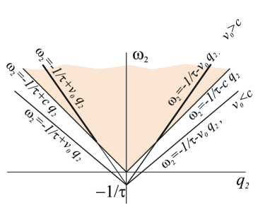
Figure 2: The branch points are arranged on the lines $\omega_{2}=-1/\tau\pm v_{0}\,q_{2}$ which intersect the forbidden region (41), i. e. $\omega_{2}>c\,|q_{2}|$, if and only if $v_{0}>c$.

If $p_{0}$, $m$ and $v_{0}$ are connected by the relativistic relation, then $v_{0}<c\,$ and a simple inspection of Figure 2 reveals that the branch points lie outside the region (41). However, if the non-relativistic relation $v_{0}=p_{0}/m\,$ is taken, then $v_{0}\,$ is not bounded and, provided that the electron density is high enough (large $p_{0}$), $v_{0}>c$, the region ${\mathbb{I}}{\rm m}\,(\omega)>|{\mathbb{I}}{\rm m}\,(q)|$ contains an infinite number of branch points —as it is illustrated in Figure 2— and the FS-causality condition is violated,

(ii)

both functions seem to have a pole at $q=0$ but this is a false singularity in both cases. Indeed, as $\omega+i/\tau\neq 0\,$, we can substitute the Taylor expansion of the logarithm around $q=0$ in equations (53-54) to obtain neat Taylor series

$$\chi^{L}(q,\omega)=-\frac{\omega_{\rm p}^{2}mv_{0}}{4\pi p_{0}\,\left(\omega+i/\tau\right)^{2}}+O(q^{2})\qquad{\rm and}\qquad\chi^{T}(q,\omega)=-\frac{\omega_{\rm p}^{2}mv_{0}}{4\pi p_{0}\,\omega\left(\omega+i/\tau\right)}+O(q^{2})\,,$$

and finally

(iii)

the transverse function presents a pole at $\omega=0\,$ which lies inside the allowed region (42).

If $q=0$, both susceptibilities present a pole at $\omega=-i/\tau\,$ but, if $\tau\neq\infty\,$, $\;\displaystyle{{\mathbb{I}}{\rm m}\,(\omega)=-\frac{1}{\tau}\leq 0=c\,|{\mathbb{I}}{\rm m}\,(q)|\,}$, which lies inside the allowed region (42).

The right asymptotic behavior of $q\,\chi(q,\omega)=h(k_{+},k_{-})\,$ for large $k_{\pm}\,$ is crucial to derive the integral relation (50) from the fact that $q\,\chi(q,\omega)$ has no singularities in the region (41), as it happens when $v_{0}<c$. Substituting

$$\omega=\frac{c(k_{+}+k_{-})}{2}\,,\qquad q=\frac{k_{+}-k_{-}}{2}$$

into equations (53-54) in the non-relativistic regime ($v_{0}\ll c$), this leads to the asymptotic expansion $\,h^{A}(k_{+},k_{-})=q\,\chi^{A}(q,\omega)=O(k_{+}^{-1})\,,\quad A=L,\,T\,$, which is sufficient to derive the integral expression (45).

In the present case a straight evaluation, which involves Spence dilogarithm functions, shows that both $\chi^{L}$ and $\chi^{T}$ satisfy the integral relation (45).

It is worth noticing that the functions (53-54) do not meet the asymptotic behavior (31). This is because the hypothesis of Theorem 1 is not met. Indeed, the latter includes the vanishing of $G(u^{+},u^{-})$ when any of the two variables is negative, i. e. FS-causality, and its continuity in this domain. Restricting to the FS-causal case, with damping time $\tau=\infty$ and $\,v_{0}<c\,$, the inversion of the Fourier transform (14) for the longitudinal function is a short calculation that yields

$$\tilde{\chi}^{L}(r,t)=\frac{\pi}{|r|}\,\delta(t)+\frac{\pi}{v_{0}t^{2}}\,\Theta(v_{0}t-|r|)$$

and none of both terms is a continuous function in the region $ct\geq|r|\,$, i. e. $u^{\pm}\geq 0\,$. Moreover, in the case $v_{0}=c\,$, the second term is a continuous function for $t>|r|/v_{0}\,$ but it starts abruptly in the boundary.

4.2 Non-relativistic quantum degenerate electron gas (random phase approximation)

Lindhard [4] also derives both the longitudinal and transverse dielectric functions for the non-relativistic quantum model of a Fermi electron gas at zero temperature. The susceptibilities are

$$\chi^{L}(q,\omega)=\frac{3\omega_{\rm p}^{2}}{8\pi\,q^{2}v_{0}^{2}}\,f^{L}(z,u)\qquad{\rm and}\qquad\chi^{T}(q,\omega)=-\frac{3\omega_{\rm p}^{2}}{32\pi\,\omega^{2}}\,f^{T}(z,u)$$ (55)

with

$$f^{L}(z,u)=1+\frac{1-(z-u)^{2}}{4z}\,\log\frac{z-u+1}{z-u-1}+\frac{1-(z+u)^{2}}{4z}\,\log\frac{z+u+1}{z+u-1}$$ (56)

and

$$f^{T}(z,u)=1+3u^{2}+z^{2}-\frac{\left[1-(z-u)^{2}\right]^{2}}{4z}\,\log\frac{z-u+1}{z-u-1}-\frac{\left[1-(z+u)^{2}\right]^{2}}{4z}\,\log\frac{z+u+1}{z+u-1}$$ (57)

where the dimensionless variables

$$z=\frac{q}{2q_{0}}\,,\qquad u=\frac{\omega^{\prime}}{q\,v_{0}}\,,\qquad\omega^{\prime}=\omega+i\frac{\gamma}{\hbar}\,,$$ (58)

have been used and $v_{0}$ and $\hbar q_{0}\,$ are the values of the velocity and momentum at the Fermi surface.

As for the singularities of $\chi(q,\omega)\,$ we find that:

$q=0$,

or $z=0\,$, is only an apparent singularity of $\chi^{L}\,$. Indeed, puting $u=y/z\,$, with $\,\displaystyle{y=\frac{\omega^{\prime}}{2\,q_{0}\,v_{0}}}\,$, writing the logarithm terms as

$$\log\left(1\mp\displaystyle{\frac{z^{2}+z}{y}}\right)-\log\left(1\mp\displaystyle{\frac{z^{2}-z}{y}}\right)$$

and taking the Taylor expansion $\log(1+x)=x-x^{2}/2+O(x^{3})\,$, we easily arrive at $\,f^{L}(z,u)=-{z^{2}}/{y^{2}}+O(z^{3})\,$ and, including (55), we see that $\,\displaystyle{\chi^{L}(q,\omega)=-\frac{3\omega_{\rm p}^{2}}{8\pi\omega^{\prime\,2}}+O(q)}\,$, which has no singularity at $\,q=0\,$.

$\omega=0$,

is a pole of $\chi^{T}(q,\omega)\,$, but it is outside the region $\,{\mathbb{I}}{\rm m}\,(\omega)>c\,|{\mathbb{I}}{\rm m}\,(q)|\,$.

Branch points

at $\,z+\sigma\,u+\lambda=0\,$, with $\,\sigma,\lambda=\pm 1\,$ which, including (58), amounts to

$$\left(q+\lambda q_{0}\right)^{2}-q_{0}^{2}+\frac{2\sigma m\omega^{\prime}}{\hbar}=0$$

or, separating the real and imaginary parts, $\,q=q_{1}+i\,q_{2}$ and $\,\omega=\omega_{1}+i\,\omega_{2}\,$, we have that

$$\omega_{2}=-\sigma s_{1}s_{2}\,\frac{\hbar}{m}\,\left(|q_{1}|+\lambda s_{1}q_{0}\right)\,|q_{2}|-\frac{\gamma}{\hbar}\,,$$ (59)

where $\,s_{j}={\rm sign}\,q_{j}\,$. In the forbidden region $\,\omega_{2}>c\,|q_{2}|\,$ this equation amounts to

$$-\sigma s_{1}s_{2}\,\frac{\hbar}{m}\,\left(|q_{1}|+\lambda s_{1}q_{0}\right)>1+\frac{\gamma}{\hbar|q_{2}|c}$$

which admits the solution

$$s_{2}=-\sigma s_{1}\qquad{\rm and}\qquad|q_{1}|+\lambda s_{1}q_{0}>\frac{m}{\hbar}\,\left(1+\frac{\gamma}{\hbar|q_{2}|c}\right)\,$$

if, and only if, $\,q_{2}\neq 0\,$. Hence both $\chi^{L}$ and $\chi^{T}$ present branch points in the region (41) and therefore Lindhard dielectric functions (55) violate the FS-causality condition, regardless of the magnitude of the Fermi momentum.

Notice that the latter is consistent with the fact that Lindhard dielectric functions fulfill the Kramers-Kronig relations for real $\,\omega\,$ and $\,q\,$, because in this case $\,q_{2}=0\,$ and $\omega_{2}<0\,$, which falls outside the domain (41).

4.3 Valence electrons in semiconductors and insulators

Levine and Louie [27] derived a model dielectric function by adding a lowest excitation frequency (or “gap”) into the Lindhard dielectric function $\,\varepsilon^{L}(q,\omega)\,$. They first modified the imaginary part of the function and used the standard Kramers-Kronig relations to derive the real part and the result is an expression for $\,\varepsilon^{L}(q,\omega)\,$ for real values of $q$ and $\omega\,$. A closed expression for complex valued $q$ and $\omega$ can be obtained by replacing $\omega$ with $\,\sqrt{\omega^{2}-\omega_{g}^{2}}\,$ in the expressions (55-58). The resulting dielectric function presents the same false pole at $q=0$, two extra branch points at $\pm\omega_{g}\,$ which is real and other branch points at

$$\left(q+\lambda q_{0}\right)^{2}-q_{0}^{2}=-\frac{2\sigma m}{\hbar}\,\sqrt{\omega^{2}-\omega_{g}^{2}}\,,\qquad\quad\lambda,\,\sigma=\pm 1$$

For real values of $q$, the right hand side is real, which implies that $\omega$ is real as well. For $q=q_{1}+iq_{2}\,,\quad q_{2}\neq 0\,$, examining the imaginary part of the square of the above equation we easily obtain

$$\frac{\omega_{2}}{q_{2}}=\frac{\hbar^{2}(q_{1}+\lambda q_{0})}{m^{2}\omega_{1}}\,\left[(q_{1}+\lambda q_{0})^{2}-q_{0}^{2}-q_{2}^{2}\right]\,,$$

whence it follows that there are branch points in the forbidden region (41) and therefore the dielectric function of Levine and Louie violates FS-causality.

4.4 Relativistic quantum degenerate electron gas

The dielectric functions $\varepsilon^{L}(q,\omega)$ and $\varepsilon^{T}(q,\omega)$ of an electron gas within a quantum electrodynamics framework (for real positive values of $q$ and $\omega$) were derived by Jancovici [28]. He gave both the real and imaginary parts, respectively equations (A.1) and (A.1’) in [28], for the longitudinal dielectric function, and (A.4) and (A.4’) for the transverse function.

We shall here analyze the longitudinal dielectric function whose analytic extension to complex $q$ and $\omega$ is (in natural units, $\hbar=c=1$)

$$\varepsilon^{L}=\varepsilon^{\prime}_{0}+\frac{2e^{2}}{3\pi}\left(\frac{4q_{0}^{2}\beta_{0}^{-1}}{q^{2}}-\log\frac{1+\beta_{0}^{-1}}{\mu_{0}}\right)+A\,\log\frac{Q_{+}}{Q_{-}}+B\,\log\frac{N_{+}}{N_{-}}+C\,\log\frac{P_{+}}{P_{-}}$$

where $q_{0}$ is the Fermi momentum, $\beta_{0}$ is the Fermi velocity,

$$\beta_{0}^{-1}=\sqrt{1+\mu_{0}^{2}}\,,\qquad\qquad\mu_{0}=mc/q_{0}=\gamma_{0}^{-1}\,\beta_{0}^{-1}\qquad$$

$$A = \frac{e^{2}(q^{2}c^{2}-\omega^{2}-2m^{2}c^{4})}{6\pi(q^{2}c^{2}-\omega^{2})}\sqrt{\frac{q^{2}c^{2}-\omega^{2}+4m^{2}c^{4}}{q^{2}c^{2}-\omega^{2}}}$$

$$Q_{\lambda} = \left[(q^{2}c^{2}-\omega^{2})q_{0}\beta_{0}^{-1}+\lambda q_{0}\sqrt{(q^{2}c^{2}-\omega^{2})(q^{2}c^{2}-\omega^{2}+4m^{2}c^{4})}\right]^{2}-4m^{4}\omega^{2}c^{6}\,,\qquad\lambda=\pm 1$$

$$B = \frac{e^{2}\,\omega}{\pi cq^{3}}\,\left(\frac{q^{2}}{4}-\frac{\omega^{2}}{12c^{2}}-q_{0}^{2}\beta_{0}^{-2}\right)\,,\qquad\qquad\quad N_{\lambda}=4q_{0}^{2}c^{2}(qc+\lambda\omega\beta_{0}^{-2})-(q^{2}c^{2}-\omega^{2})^{2}$$

$$C = \frac{e^{2}\,q_{0}\beta_{0}^{-1}}{\pi c^{2}q^{3}}\,\left[\frac{2}{3}q_{0}^{2}\beta_{0}^{-2}c^{2}-\frac{1}{2}(q^{2}c^{2}-\omega^{2})\right]\,,\qquad\quad P_{\lambda}=\left[2qq_{0}c^{2}+\lambda(q^{2}c^{2}-\omega^{2})\right]^{2}-4\omega^{2}q_{0}^{2}\beta_{0}^{-2}c^{2}$$

and

$$\varepsilon^{\prime}_{0} = 1+\frac{e^{2}}{3\pi}\,\left(\frac{5}{3}-\frac{4q_{0}^{2}\mu_{0}^{2}c^{2}}{q^{2}c^{2}-\omega^{2}}\right)-4\,A\,\ln\left(\sqrt{\frac{q^{2}c^{2}-\omega^{2}}{4m^{2}c^{4}}}+\sqrt{\frac{q^{2}c^{2}-\omega^{2}+4m^{2}c^{4}}{4m^{2}c^{4}}}\right)$$

For the sake of convenience, we translate these expressions into the dimensionless variables

$$z=\frac{q}{2q_{0}}\,,\qquad u^{\prime}=\frac{\omega}{2\,c\,q_{0}}\,\qquad{\rm and}\qquad\zeta=\gamma_{0}\,\beta_{0}\,\sqrt{z^{2}-u^{\prime 2}}$$ (60)

and, after some manipulation, we obtain

$$\varepsilon^{L}=\varepsilon^{\prime}_{0}+\frac{2e^{2}}{3\pi}\left(\frac{\beta_{0}^{-1}}{z^{2}}-\frac{1}{2}\,\log\frac{1-\beta}{1+\beta}\right)+A\,\log\frac{m_{++}m_{+-}}{m_{-+}m_{--}}+\sum_{\lambda=\pm}B_{\lambda}\,\log\frac{n_{\lambda+}}{n_{\lambda-}}$$ (61)

with

$$A = \frac{e^{2}}{6\pi}\,\left(1-\frac{1}{2\,\zeta^{2}}\right)\,\sqrt{1+\frac{1}{\zeta^{2}}}$$ (62)

$$m_{\tau\nu} = \nu z+\zeta^{2}+\tau\,\beta_{0}^{-1}\,\zeta\,\sqrt{1+\zeta^{2}}\,,\qquad\tau\,,\;\nu=\pm 1$$ (63)

$$B_{\lambda} = \frac{e^{2}(\beta_{0}^{-1}+\lambda u^{\prime})}{12\pi z^{3}}\,\left[(\beta_{0}^{-1}+\lambda u^{\prime})^{2}-3z^{2}\right]$$ (64)

$$n_{\lambda\sigma} = u^{\prime}(u^{\prime}+\lambda\beta_{0}^{-1})-z(z+\sigma)\,,\qquad\qquad\lambda,\,\sigma=\pm 1$$ (65)

and

$$\varepsilon^{\prime}_{0}=1+\frac{e^{2}}{3\pi}\,\left(\frac{5}{3}-\frac{1}{\zeta^{2}}\right)-4\,A\,\ln\left(\zeta+\sqrt{1+\zeta^{2}}\right)$$ (66)

Consider now (61) as a function of the complex variables $z$ and $u^{\prime}$. The possible singularities are

a pole

at $z=0$, which is a false singularity as is revealed by the Taylor expansion (Mathematica)

$$\varepsilon^{L} = 1+\frac{5e^{2}}{9\pi}+\frac{e^{2}\,(\mu_{0}-\beta_{0}^{-1})}{3\pi\,u^{\prime\,2}}-\frac{2e^{2}}{3\pi}\,\ln\frac{1+\beta_{0}^{-1}}{\mu_{0}}+\frac{e^{2}\,(\mu_{0}^{2}+2u^{\prime\,2})\sqrt{u^{\prime\,2}-\mu_{0}^{2}}}{6\pi\,u^{\prime\,3}}\,\times$$

$$\left[-2\,\ln\frac{\sqrt{-u^{\prime\,2}}+\sqrt{-u^{\prime\,2}+\mu_{0}^{2}}}{\mu_{0}}+\ln\frac{\beta_{0}u^{\prime}-\sqrt{u^{\prime\,2}-\mu_{0}^{2}}}{\beta_{0}u^{\prime}+\sqrt{u^{\prime\,2}-\mu_{0}^{2}}}\right]+O(z^{2})$$

This has a singularity at $u^{\prime}=0$ but, as $z=0$, this implies that there is a singularity at $u^{\prime}=z=0$ or, in terms of the light cone frequencies (15), $k_{+}=k_{-}=0\,$, which is outside the region $\,{\mathbb{I}}{\rm m}\,(k_{\pm})>0\,$. Recall that this is the region $\,{\mathbb{I}}{\rm m}\,(\omega)>c\,|{\mathbb{I}}{\rm m}\,(q)|\,$ —see Section 2.3, eq. (41).

a pole (or branch point)

at $\,\displaystyle{\zeta^{2}=-\frac{k_{+}k_{-}}{4m^{2}c^{2}}=0}\,$, which is outside the region $\,{\mathbb{I}}{\rm m}\,(k_{\pm})>0\,$.

branch points

at $\,n_{\lambda\sigma}=0$. In terms of the light cone frequencies (65) becomes

$$n_{\lambda\sigma}\equiv\left[k_{+}+(\lambda\beta^{-1}_{0}+\sigma)q_{0}\right]\,\left[k_{-}+(\lambda\beta^{-1}_{0}-\sigma)q_{0}\right]-m^{2}c^{2}=0\,.$$

Putting

$$k_{+}+(\lambda\beta^{-1}_{0}+\sigma)q_{0}=x+iy\qquad{\rm and}\qquad k_{-}+(\lambda\beta^{-1}_{0}-\sigma)q_{0}=z+it\,,$$

where ${\mathbb{I}}{\rm m}\,(k_{+})=y>0\,$ and ${\mathbb{I}}{\rm m}\,(k_{-})=t>0\,$, we have that

$$xz-yt=m^{2}c^{2}\,,\qquad\qquad xt+yz=0\,.$$

This implies that $\displaystyle{-\frac{y}{t}\,(z^{2}+t^{2})=m^{2}c^{2}}\,,$ which is impossible in the region ${\mathbb{I}}{\rm m}\,(k_{+})=y>0\,$, ${\mathbb{I}}{\rm m}\,(k_{-})=t>0\,$, i. e. the forbidden region (41).

branch points at $\,m_{\tau\nu}=0\,$.

Each of these coincides with a $n_{\lambda\sigma}=0$ for some $\lambda$ and $\sigma$. Indeed, it can be easily checked that $\,\displaystyle{\prod_{\tau,\nu=\pm}m_{\tau,\nu}=\mu_{0}^{4}\,\prod_{\lambda,\sigma=\pm}n_{\lambda\sigma}}\,$, whence it follows that one of the $m$’s vanishes if and only if one of the $n$’s does.

branch points

at $\,\zeta^{2}+1=0\,$, which amounts to $\,z^{2}+\mu_{0}^{2}-u^{2}=0\,$ or $\,k_{+}k_{-}=4m^{2}c^{2}\,$, which has no roots in the region $\,{\mathbb{I}}{\rm m}\,(k_{\pm})>0\,$.

As for the asymptotic behavior of $\varepsilon^{L}$ at large $\displaystyle{k_{\pm}=\frac{\omega}{c}\pm q}\,$, it is dominated by the logarithmic term in (66) and

$$\varepsilon_{0}^{L}\sim-\frac{e^{2}}{3\pi}\,\log(k_{+}k_{-})$$

which disagrees with the asymptotic behavior (31). This is probably due to a breakdown of the hypothesis in Theorem 1, in that the derivatives of the function $G(u^{+},u^{-})$ fail to be continuous (for $N=2$).

5 Conclusion

We have studied the consequences of the condition of causality on the general form of the susceptibility function $\chi(q,\omega)$ of an isotropic medium described within the linear response approximation (or, alternatively, the dielectric function). Due to the fact that we are beyond the optical approximation —$\varepsilon$ depends both on wave vector and frequency— the electric polarization, the effect, at one point $\mathbf{x}$ and a given instant of time $t$ depends on the values of the electric field, the causes, at space points other than $\mathbf{x}$. Hence the response of the medium involves signals propagating from the causes to the effect and causality requires that these signals do not travel faster than light in vacuum.

On the basis of merely this causality condition and the requirement that a constant finite electric field must produce a finite polarization we have proved that the extension of the dielectric function to complex values of the variables $q$ and $\omega$ must be double analytic in the region $\,c\,\left|{\mathbb{I}}{\rm m}\,(q)\right|<{\mathbb{I}}{\rm m}\,(\omega)\,$.

Furthermore, by applying asymptotic theorems for Laplace integrals, we have studied the behavior of $\,\chi\,$ for large values of $\,q\pm\omega\,$. This has required the additional assumption that the influence of the electric field at $(\mathbf{r}^{\prime},t^{\prime})$ on the polarization at $(\mathbf{r},t)$ does not start abruptly at the boundary $\,t-t^{\prime}=|\mathbf{r}-\mathbf{r}^{\prime}|/c\,$.

We have then applied the Cauchy integral formula to derive the extension of Kramers-Kronig relations to this kind of causality at a distance. This requires, as in the standard case, to assume that $\,q\,\chi(q,\omega)\,$ decays fast enough for large values of $\,|\omega\pm cq|\,$. We have recovered a generalization of Kramers-Kronig relations first obtained by Leontovich [16] for conductivity on the basis of Lorentz invariance. As a matter of fact we improve Leontovich result in that: (a) our derivation is based on more general assumptions, (b) we realize that, contrarily to Leontovich’s conjecture [16], no extra conditions apply and (c) our relations (50) must hold on the domain made explicit in that equation, which is wider than merely for real values of $q$ and $\omega$.

The analyticity conditions here obtained are to be taken as a quality test to be passed by any proposal of dielectric function, either empirical or derived from a microscopic model, in order to become acceptable on the basis of causality. Other results, e. g. the asymptotic behavior of $\,\chi(q,\omega)\,$ are less robust since their derivation is based on additional less general assumptions, e. g. the non-abrupt switch on at the boundary $\,ct\pm r=0\,$.

Often, beyond the optical approximation and to study the causal behavior of a dielectric function $\varepsilon(q,\omega)$, Kramers-Kronig relations have been checked for $q$ real and constant, whereas $\omega$ is a real variable. In that case, as ${\mathbb{I}}{\rm m}\,(q)=0\,$, our condition (42) implies that $\varepsilon(q,\omega)$ is analytic for $\,{\mathbb{I}}{\rm m}\,(\omega)>0\,$. Together with a convenient behavior at $|\omega|\rightarrow\infty\,$, the latter implies that Kramers-Kronig relations are fulfilled. However the converse is not true: the compliance with Kramers-Kronig conditions for real values of $q$ does not imply the FS-causality condition (42).

As an application we have tested several dielectric functions that are found in the literature for different microscopic models of a degenerate electron gas, whether relativistic or not. Whereas the relativistic models have already a built in FS-causality and they have succesfully passed the analyticity test, in the non-relativistic cases the success depends on the parameters of the model, e. g. if the Fermi momentum exceeds the electron mass, then the susceptibility function does not pass the FS-causality test.

Our reasoning here is based on the assumption of causality in the relations (4) and (6), which connect an input and an oputput through a response function. Relations of this kind are the basis of linear response theory. Therefore the results here derived also hold for any homogeneous, isotropic response function in the framework of any linear response theory.

Appendix

To determine the asymptotic behavior of the double Laplace integral

$$g(s_{+},s_{-})=\int_{\mathbb{R}^{+2}}{\rm d}u^{+}\,{\rm d}u^{-}\,G(u^{+},u^{-})e^{-s_{+}u^{+}-s_{-}u^{-}}$$

for large values of $\,s_{\pm}\,$ we shall prove

Theorem 1

Let $\,g(s_{+},s_{-})\,$ be the double Laplace integral (20), assume that $\,G(u^{+},u^{-})\,$ has continuous partial derivatives $\,G^{(l,j)}(u^{+},u^{-})=\partial_{+}^{l}\partial_{-}^{j}G(u^{+},u^{-})\,$ up to the $N$-th order (i. e. $l+j\leq N$) and that there exist $\,a_{\pm}\in\mathbb{R}\,$ such that

$$\,\int_{\mathbb{R}^{+2}}{\rm d}u^{+}\,{\rm d}u^{-}\,G^{(l,j)}(u^{+},u^{-})e^{-a_{+}u^{+}-a_{-}u^{-}}<\infty\,,\qquad\quad l+j\leq N\,,$$

then

$$g(\lambda s_{+},\lambda s_{-})=\sum_{0\leq l+j\leq N-1}\frac{G^{(l,j)}(0^{+},0^{+})}{\lambda^{l+j+2}s_{+}^{l+1}s_{-}^{j+1}}+o(\lambda^{-N-1})\,,\qquad\qquad\forall\lambda\in\mathbb{R}^{+}\,.$$

Consider $\,\mathcal{D}_{U,V}=[0,U]\times[0,V]\,$ and define

$$g(U,V,\mathbf{s})=\int_{\mathcal{D}_{U,V}}{\rm d}\mathbf{u}\,e^{-\mathbf{s}\cdot\mathbf{u}}\,G(\mathbf{u})=\int_{0}^{U}{\rm d}u^{+}\,e^{-s_{+}u^{+}}\,\int_{0}^{V}{\rm d}u^{-}\,e^{-s_{-}u^{-}}\,G(u^{+},u^{-})$$ (67)

It is obvious that $\,\displaystyle{g(s_{+},s_{-})=\lim_{U,V\rightarrow\infty}g(U,V,s_{+},s_{-})}\,$.

An integration by parts with respect to $u^{-}$ yields

$$g(U,V,\mathbf{s})=\frac{1}{s_{-}}\,\int_{0}^{U}{\rm d}t\,e^{-s_{+}t}\,G(t,0^{+})-\frac{e^{-s_{-}V}}{s_{-}}\,\int_{0}^{U}{\rm d}t\,e^{-s_{+}t}\,G(t,V)+\frac{1}{s_{-}}\,\int_{\mathcal{D}_{U,V}}{\rm d}\mathbf{u}\,e^{-\mathbf{s}\cdot\mathbf{u}}\,G^{(0,1)}(\mathbf{u})$$

By the hypothesis of Theorem 1, the integral in the second term on the r.h.s. is bounded if $\,{\mathbb{R}}{\rm e}\,(s_{\pm})>a_{\pm}\,$, hence the limit for $U,V\rightarrow\infty$ yields

$$g(\mathbf{s})=\frac{1}{s_{-}}\,\int_{0}^{\infty}{\rm d}t\,e^{-s_{+}t}\,G(t,0^{+})+\frac{1}{s_{-}}\,\int_{\mathbb{R}^{+2}}{\rm d}\mathbf{u}\,e^{-\mathbf{s}\cdot\mathbf{u}}\,G^{(0,1)}(\mathbf{u})$$ (68)

and, by iterating (68) as many times as permitted by the differentiability of $G$, we prove the following

Lemma 1

Assuming the hypothesis of Theorem 1,

$$g(\mathbf{s})=\sum_{k=0}^{N-1}\,\int_{0}^{\infty}{\rm d}t\,e^{-s_{+}t}\,\frac{G^{(0,k)}(t,0^{+})}{s_{-}^{k+1}}+g_{N}(\mathbf{s})$$ (69)

with $\,{\mathbb{R}}{\rm e}\,(s_{\pm})>a_{\pm}\,$ and

$$g_{N}(\mathbf{s})=\frac{1}{s_{-}^{N}}\,\int_{\mathbb{R}^{+2}}{\rm d}\mathbf{u}\,e^{-\mathbf{s}\cdot\mathbf{u}}\,G^{(0,N)}(\mathbf{u})$$

Notice also that for $j+l\leq N\,$ the hypothesis of Theorem 1 implies that it exists $\,M_{jl}\,$ such that $\left|G^{(j,l)}(\mathbf{u})e^{-a_{-}u^{-}-a_{+}u^{+}}\right|<M_{jl}\,$, and therefore

$$\left|\int_{\mathbb{R}^{+2}}G^{(j,l)}(\mathbf{u})e^{-\mathbf{a}\cdot\mathbf{u}}\,{\rm d}\mathbf{u}\right|<\int_{\mathbb{R}^{+2}}M_{jl}\,\left|e^{-(\mathbf{s}-\mathbf{a})\cdot\mathbf{u}}\right|\,{\rm d}\mathbf{u}=\frac{M_{jl}}{(\rho_{+}-a_{+})(\rho_{-}-a_{-})}$$

where $\,\rho_{\pm}={\mathbb{R}}{\rm e}\,(s_{\pm})>a_{\pm}$. In particular, for $j=0$ and $l=N$, we have that

$$\left|g_{N}(\lambda\mathbf{s})\right|<\frac{M_{0N}}{\lambda^{N}|s_{-}|^{N}(\lambda\rho_{+}-a_{+})(\lambda\rho_{-}-a_{-})}$$

whence it follows that $\,g_{N}(\lambda\mathbf{s})=o(\lambda^{-N-1})\,$, that is $\,\displaystyle{\lim_{\lambda\rightarrow\infty}g_{N}(\lambda\mathbf{s})\,\lambda^{N+1}=0}\,$.

To complete the proof of Theorem 1 we must evaluate each term in the sum on the r.h.s. of equation (69). By a result in ref. [26] we have that, under the conditions of the hypothesis,

$$\int_{0}^{\infty}{\rm d}t\,e^{-s_{+}t}\,G^{(0,k)}(t,0^{+})=\sum_{l=0}^{N-k}\frac{G^{(l,k)}(0^{+},0^{+})}{s_{+}^{l+1}}+o\left(\frac{1}{s_{+}^{N-k}}\right)$$

which, substituted into (69) leads to the sought for result

$$g(\lambda s_{+},\lambda s_{-})=\sum_{k=0}^{N-1}\sum_{l=0}^{N-k}\frac{G^{(l,k)}(0^{+},0^{+})}{\lambda^{l+k+2}s_{+}^{l+1}s_{-}^{k+1}}+o(\lambda^{-N-1})\,,\qquad\qquad\forall\lambda\in\mathbb{R}^{+}$$

References

- [1] Jackson J D, Classical Electrodynamics, John Wiley 1999
- [2] Zangwill A, Modern Electrodynamics, Chapter 18, Cambridge University Press (2012)
- [3] see, e. g., Shiles E, Sasaki T, Inokuti M and Smith D Y, Phys Rev B 22 (1980) 1612
- [4] Lindhard J, Dan Mat Fys Medd 28 (1954) 1
- [5] Penn D R, Phys Rev B 35 (1987) 482
- [6] Mermin N D, Phys Rev B 1 (1970) 2362
- [7] Tanuma S, Powell C J and Penn D R (2004), Calculations of electron inelastic mean free paths. VIII. Data for 15 elemental solids over the 50–2000 eV range, Surface and Interface Analysis 36 (2004) 1
- [8] Fernández-Varea J M, Salvat F, Dingfelder M and Liljequist D, Nucl Instrum Meth B 229 (2005) 187
- [9] Sorini A P, Kas J J, Rehr J J, Prange M P and Levine Z H, Phys Rev B74 (2006) 165111
- [10] Da B, Shinotsuka H, Yoshikawa H, Ding Z and Tanuma S, Phys Rev Lett 113 (2014) 063201
- [11] Vladimirov V S, Equations of Mathematical Physics, Mir Publishers 1984
- [12] Nussenzveig H M, Causality and dispersion relations, Academic Press (1972)
- [13] Schützer W and Tiomno J, Phys Rev 83 (1951) 249
- [14] van Kampen N G, Phys Rev 89 (1953) 1072
- [15] Toll J S, Phys Rev 104 (1956) 1760
- [16] Leontovich M, Sov Phys JETP 13(1961) 634
- [17] Melrose D B and Stoneham R J, J Phys A: Math Gen, 10 (1977) L17
- [18] Sun J G and Puri A, Optics Communications, 70 (1989) 33
- [19] Thoma M H, Eur Phys J C , 16 (2000) 513
- [20] Shokri B and Rukhadze A A, Electrodynamics of Conducting Dispersive Media, Springer Series on Atomic, Optical, and Plasma Physics, vol 111, Springer (Cham, 2019)
- [21] Rozanov N N, Optics and Spectrosopy, 97 (2004) 280
- [22] Kirzhnits D A, Pis’ma Zh Eksp Teor Fiz, 46 (1987) 244
- [23] Jackson J D, Op. cit., §7.10.C
- [24] Titchmarsh E C, Introduction to the theory of Fourier integrals, Chap 5, Clarendon Press 1948
- [25] Detman J W, Applied Complex Variables, Chap 3, Dover 1984
- [26] Erdélyi A, Asymptotic expansions, sect. §2.2, Dover 1956
- [27] Levine Z H and Louie S G, Phys Rev B25 (1982) 6310
- [28] Jancovici B, Nuovo Cimento 25 (1962) 428