Reduced qKZ equation: general case
Abstract.
We use the quantum group approach for the investigation of correlation functions of integrable vertex models and spin chains. For the inhomogeneous reduced density matrix in case of an arbitrary simple Lie algebra we find functional equations of the form of the reduced quantum Knizhnik-Zamolodchikov equation. This equation is the starting point for the investigation of correlation functions at arbitrary temperature and notably for the ground state.
1. Introduction
In this paper we derive a difference-type functional equation, called the discrete reduced quantum Knizhnik–Zamolodchikov equation, for the density operator of a quantum integrable vertex model related to an arbitrary complex simple Lie algebra. Our setting allows for the study of correlation functions at finite and zero temperature in the thermodynamic limit, or alternatively of ground-state correlators on finite ring shaped and infinite chains. Throughout this paper we use methods based on the notion of a quantum group introduced by Drinfeld [1] and Jimbo [2]. To be precise, we consider quantum integrable systems related to a special class of quantum groups, namely the quantum loop algebras, see section 2.2 for the definition.
Our work aims at extending the previous work, see [3, 4] and later developments, related to systems based on the quantum loop algebra which enjoys a simple crossing symmetry due to the equivalence of any representation with its dual. Some explorative investigations for a system based on the first fundamental representation of allowed for the computation of nearest and next-nearest neighbour correlators for the associated quantum spin chain of XXX-type in the ground-state [5, 6]. In these works the necessity of dealing simultaneously with at least two different representations of the same quantum group became obvious. Furthermore, unitarity conditions involving different representations, and crossing relations for representations dual to each other appeared. Here we put such constructions on solid systematic grounds valid for arbitrary representations of any quantum group. Our constructions will allow for a uniformized investigation of correlation functions making ad-hoc constructions obsolete.
The central object of the quantum group approach is the universal -matrix being an element of the tensor product of two copies of the quantum loop algebra. The integrability objects are constructed by choosing representations for the factors of that tensor product.111For the corresponding terminology we refer to our paper [7]. The consistent application of the method for constructing integrability objects and proving their properties was initiated by Bazhanov, Lukyanov and Zamolodchikov [8, 9, 10]. They studied the quantum version of KdV theory. Later on the method proved to be efficient for studying other quantum integrable models. Accordingly, within the framework of this approach, -operators [11, 12, 13, 14, 15, 16, 17], monodromy operators and -operators were constructed [18, 16, 17, 19, 20, 7]. The corresponding sets of functional relations were found and proved [21, 22, 18, 7, 23, 24].
To derive the reduced qKZ equation one needs some special properties of the integrability object related to the quantum loop algebra under consideration. Namely, one uses the unitarity relations, crossing relations and the so-called initial condition. It appears that these relations, apart from the initial condition, follow from the properties of the universal -matrix. The detailed discussion can be found in paper [25], see also paper [26].
The plan of the paper is as follows. In section 2 we introduce a quantum loop algebra, its universal -matrix, and define the basic integrability objects called -operators. Then we describe the properties of -operators, such as the unitarity and crossing relations, necessary for the subsequent derivation of the reduced qKZ equation. This section is concluded by the definition of monodromy and transfer operators.
In section 3 we discuss the construction of the Hamiltonian of the system as a member of the system of commuting quantities. The aforementioned initial condition is also given here. We introduce a convenient normalization of the -operators which leads to a simple form of the crossing and unitarity relations. Also the initial condition becomes simple. Then we remind of the definition of the density operator and represent it as the Trotter limit of some sequence of operators. Such a representation allows us to relate the density operator to the partition sum of some square lattice vertex model with the free horizontal boundaries.
A graphical derivation of the reduced qKZ equation is described in section 4, and the corresponding pictures with appropriate comments are placed in the appendix.
2. Quantum loop algebras and integrability objects
2.1. Preliminaries on Lie algebras
Let be a complex finite dimensional simple Lie algebra of rank [27, 28], a Cartan subalgebra of , and the root system of relative to . Fix a system of simple roots , . It is known that the corresponding coroots form a basis of , so that
The Cartan matrix of is defined by the equation
Denote by the highest root of [27, 28]. We have
for some positive integers and with . These integers, together with
are the Kac labels and the dual Kac labels of the Dynkin diagram associated with the extended Cartan matrix . Recall that the sums
are called the Coxeter number and the dual Coxeter number of .
Denote by the Cartan subalgebra of extended by a one dimensional center . We consider the simple roots , , as elements of assuming that
Introduce an additional ‘root’
and an additional ‘coroot’
After that for the entries of the extended Cartan matrix of we have the expression
2.2. Quantum loop algebras
Let be a nonzero complex number such that is not a root of unity. We assume that
for any . As usually, we define the -deformation of a number as
Note that the extended Cartan matrix is symmetrizable. It means that there exists a diagonal matrix , where , , are positive integers, such that the matrix is symmetric. Such a matrix is defined up to a nonzero scalar factor. We fix the integers assuming that they are relatively prime and denote
The quantum loop algebra is a unital associative -algebra generated by the elements
satisfying the relations
| (2.1) | |||
| (2.2) | |||
| (2.3) | |||
| (2.4) |
Here, relations (2.2) and (2.3) are valid for all . The last line of the relations is valid for all distinct .
The quantum loop algebra is a Hopf algebra. Here the multiplication mapping is defined as
and for the unit mapping we have
The comultiplication , the antipode , and the counit are given by the relations
| (2.5) | |||
| (2.6) | |||
| (2.7) |
For the inverse of the antipode one has
| (2.8) |
2.3. Universal -matrix
Let be the automorphism of the tensor square of the algebra defined by the equation
It is known that the mapping
is a comultiplication in called the opposite comultiplication.
Let be a quantum loop algebra. There exists a unique element of the tensor product of connecting the two comultiplications as
for any , and satisfying in the equations
The meaning of the superscripts in the above relations is explained in any textbook on quantum groups, see also the appendix of paper [25]. The element is called the universal -matrix. One can show that it satisfies the universal Yang-Baxter equation
in .
There are two main approaches to the construction of the universal -matrix for a quantum loop algebra. One of them was proposed by Khoroshkin and Tolstoy [29, 11, 30, 31], and another one is related to the names of Beck and Damiani [32, 33]. It should be noted that we define the quantum loop algebra as a -algebra. It can be also defined as a -algebra, where is considered as an indeterminate. In this case one really has the universal -matrix. In our case, the universal -matrix exists only in some restricted sense, see, for example, paper [34], and the corresponding discussion in paper [25] for the case of .
As for any Hopf algebra, starting from two representations of , say and , we construct a new representation of by the relation
The corresponding -module is denoted by , where and are the modules corresponding to the representations and .
2.4. Spectral parameter
In applications to the theory of quantum integrable systems, one usually considers families of representations of a quantum loop algebra parametrized by a complex parameter called a spectral parameter. We introduce a spectral parameter in the following way. Assume that the quantum loop algebra is -graded,
so that any element can be uniquely represented as
Given , we define the grading automorphism by the equation
It is worth noting that
| (2.9) |
for any . Now, for any representation of we define the corresponding family of representations as
If is the -module corresponding to the representation , we denote by the -module corresponding to the representation .
The common way to endow by a -gradation is to assume that
where are arbitrary integers. It is clear that for such a -gradation one has
We denote
where, as above, are the Kac labels of the Dynkin diagram associated with the extended Cartan matrix of .
2.5. -operators
Now recall the definition of an -operator. Let and be -modules and and the corresponding representations of .222In this paper we assume that all -modules under consideration are finite dimensional. The -operator is defined as
Here and are spectral parameters, and the normalization factor.
Using (2.9) and (2.10), one can demonstrate that
for any . Therefore, under an appropriate choice of the normalization factor, depends only on the combination and one can use -operators depending on only one spectral parameter. Below we always use this choice of the normalization, however, for our purposes it is more convenient to consider -operators as depending on two spectral parameters.
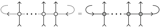
We use for the matrix elements of the depiction which can be seen in figure 2.2.
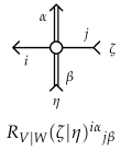
Here we associate with and a single and a double lines respectively. It is worth to note that the indices in the graphical image go clockwise.
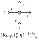
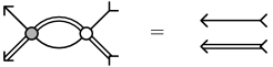
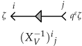
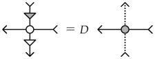
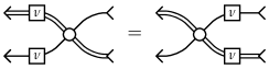
For the matrix elements of the inverse of the -operator we use the depiction given in figure 2.2. Here we use a grayed circle for the operator and the counter-clockwise order for the indices. This allows one to have a natural graphical form of the equation
see figure 2.3.
2.6. Unitarity relations
Let the -modules and are such that the module is simple for general values of the spectral parameters and . In this case the following unitarity relation
is valid. Here and in similar cases below we use the notations
with and being the permutation operators on the corresponding tensor products.
2.7. Crossing relations
For any finite dimensional -module one has two dual modules. One dual module is denoted by and is defined with the help of the antipode , another one is denoted by and is defined with the help of the inverse of the antipode .
By a crossing relation we mean any relation connecting an -operator with an -operator for which one of the modules and (or both) is (are) replaced by a dual module. In this paper we will use the following three crossing relations. The first one is
| (2.11) |
and the second one is
| (2.12) |
The double dual representation is isomorphic to up to a redefinition of the spectral parameter. This leads to the third crossing relation. To describe it, we introduce the following element
of , see [25]. Here are the matrix elements of the matrix inverse to the Cartan matrix of the Lie algebra , and denotes invariant nondegenerate symmetric bilinear form on normalized by the equation
Now one can demonstrate that
| (2.13) |
where
This is the third crossing relation we need. More crossing relations and the corresponding proofs can be found in paper [25].
2.8. Monodromy and transfer operators
In the theory of quantum integrable statistical systems the matrix elements of an -operator are treated as weights of the vertices of a square lattice. To find the corresponding partition function one introduces monodromy operators and the corresponding transfer operators. To define a monodromy operator we use instead of the -module , used in the definition of the -operators, the -module
| (2.14) |
and define the monodromy operator as
Using properties of the universal -matrix one can see that
| (2.15) |
Here the meaning of the superscripts can be found again in any textbook on quantum groups. The factors of the tensor product (2.14) are numbered from left to right. The graphical representation of the matrix elements of the monodromy operator for the case can be found in figure 2.4.
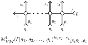
The modification needed for the general case is evident.
The transfer operator corresponding to the monodromy operator (2.15) is defined by the equation
| (2.16) |
with the depiction for the case given in figure 2.5.
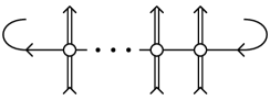
Here means the partial trace with respect to the space , see, for example, the appendix of paper [25], and hooks at the ends of the line mean that it is closed in an evident way. The most important property of transfer operators is their commutativity
| (2.17) |
It is the source of commuting quantities of quantum integrable systems.
3. Density operator
3.1. Commuting quantities and Hamiltonian
The transfer operator (2.16) acts on the -module . As a vector space it is just . We assume that and construct commuting quantities on as follows. First of all we denote
It follows from (2.17) that the quantities
commute,
| (3.1) |
In fact we have one more operator which commutes with all .
The usual choice for the Hamiltonian is
Assume that the initial condition
| (3.2) |
is valid for some nonzero constant . Here, as above, is the permutation operator on . One can demonstrate that in this case
| (3.3) |
where we assume that
Thus, we have a local Hamiltonian. For the well known simple graphical derivation of relation (3.3) we refer to paper [25].
3.2. Normalization
In this paper we work with a fixed -module and its dual . We choose the normalization of , and assuming that
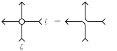
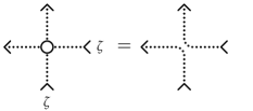
In this case the crossing relation (2.11) implies

The graphical image of these relations can be found in figures 3.2 and 3.2. Here and below, for the representation we use the dotted variant of the line used for the representation .
It is clear that the crossing relation (2.12) takes the form
| (3.4) |
and has the graphical image given in figure 3.3.
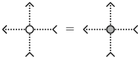
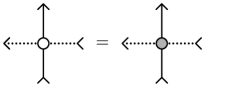
Starting from the crossing relation (2.13), we obtain in the case under consideration two equations
| (3.5) | |||
| (3.6) |
where
| (3.7) |
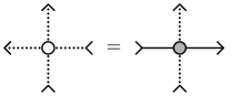
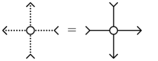
To give a graphical interpretation of these equations, we use for the matrix elements of the operator and its inverse the depiction given in figures 3.5 and 3.5.
It can be demonstrated now that figures 3.7 and 3.7 represent the crossing relations (3.5) and (3.6).

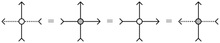
We choose the normalization factor so that the matrix elements of are rational functions of the spectral parameters, and satisfies the unitarity relation
| (3.8) |
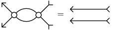
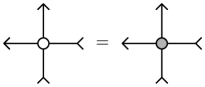
see [35, Propositions 9.5.3 and 9.5.5]. We give the graphical form of this relation and the equivalent one in figures 3.9 and 3.9.
The crossing relation (3.4) and the unitarity relation (3.8) lead to the unitarity relations in figures 3.11 and 3.11.

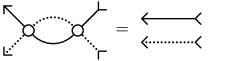
Using the equations depicted in figures 3.2, 3.9 and 3.3, 3.2 we come to the chain of equalities given in figure 3.12.
We see that the -operators and satisfy the unitarity relation given in figure 3.14, or the equivalent relation in figure 3.14.
Finally we assume that the initial condition (3.2) is satisfied. It follows from the unitarity relation (3.8) that in our case
Possibly changing the sign of , without destroying the form of the unitarity and crossing relations, we make equal to . The resulting initial condition is depicted in figure 3.16.
3.3. Density operator
The density operator of a quantum statistical system with the Hamiltonian is given by the equation
where is the partition function of the system defined as
The expectation value of an arbitrary observable is
Let us exploit the relation of the Hamiltonian with the transfer operator . To this end we introduce the ‘additive’ spectral parameter related to the ‘multiplicative’ spectral parameter by the relation
Slightly abusing notation, we denote by the transfer operator expressed as a function of . Now we have
and it is not difficult to see that
We consider one more transfer operator related to the module and defined as
It generates one more set of commuting quantities
In fact, in addition to (3.1), we have
The operators and commute with all and all . In fact, is the left shift and is the right shift, and we have
In terms of the additive spectral parameter we have
Starting from this equation, we determine that
For any positive integer we can write
These equations give
and we see that
Denote
where
Finally, using the multiplicative spectral parameter, we obtain
| (3.10) |
It is clear that
3.4. Density operator as the partition function of a vertex model
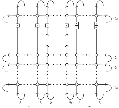
It follows from (3.10) that the matrix elements of the operator can be represented as the partition function of a vertex model on a square lattice, see figure 3.18.
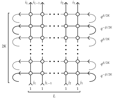
Here we have the periodic boundary conditions in the horizontal direction and open top and bottom boundaries. The thermodynamic limit would be obtained when . However, the existence of the limit over is quite problematic. Therefore, we proceed to the density operator which allows to find expectation values only for local observables. To this end we assume that , where and are positive integers. We consider as fixed and take the trace of over the first and the last spaces associated with vertical directions of the lattice. We denote the corresponding ‘density operator’ as and the corresponding ‘partition function’ as . The density operator of interest is certainly the limit as and . We assume that these limits commute, see a discussion in paper [36], so that
To go further we generalize the objects under consideration in the following way.
We have horizontal transfer operators and vertical monodromy and transfer operators defined in an evident way. We supply a horizontal transfer operator with the spectral parameters or in dependence on whether it is the operator or the operator , see figure 3.19.
The vertical monodromy operators are endowed with the spectral parameters . Thus, we consider the generalized density operator
Below, if it does not lead to misunderstanding, we omit the explicit designation of dependence on and .
After all we introduce some twisting for the vertical transfer and monodromy operators. In the framework of the quantum group approach a twisting is defined by a choice of a group-like element. Remember that an element of a Hopf algebra is called group-like if
It is clear that in our case an element
is group-like for any complex number . We denote
and use for the matrix elements of the operator and its inverse the depiction given in figures 3.21 and 3.21.


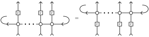
It follows from the definition of a group-like element that the operator satisfies a useful equation whose graphical image is represented by figure 3.25.

It is also clear that
This relation leads to a modified version of the graphical equation 3.25 which can be seen in figure 3.25. We also need the commutativity equation given in figure 3.26.
We introduce disorder parameters , , and twist the first vertical transfer operators. The introduction of disorder parameters regularizes the problem in the case of [37, 38]. Further, we introduce parameters , , and twist all vertical transfer and monodromy operators, see figure 3.19. This can be interpreted as turning on a ‘magnetic field’. It should be noted that all equally twisted transfer operators commute.
Denote by the horizontal space,
We use for a vertical monodromy operator, twisted with the parameters , , the notation . It acts on the space . In fact, we have
It is useful to represent a vertical monodromy operator as
where are unit operators on associated with the used basis, and the operators act on . The vertical transfer operator is defined as
It acts on the vertical space . We extend to the vertical monodromy and transfer operators the convention to omit the explicit designation of dependence on and .
Generalizing the conjecture made in [39], we assume that the transfer operators and are diagonalizable. Due to the commutativity of the vertical transfer operators with different spectral parameters , their eigenvectors can be chosen independently of . Let the eigenvectors of form a basis of the vertical space. We have
where are the corresponding eigenvalues. Denote by the vectors forming the dual basis, so that
Now we have
where instead of we write just . In a similar way we obtain
Following again paper [39], we assume that the eigenvalues and of and with the maximal absolute value are non-degenerate. In this case in the limit we get
Here we assume also that
4. Reduced qKZ equation
In this section we describe a graphical derivation of the discrete reduced qKZ equation for an arbitrary quantum loop algebra and consider the zero temperature limit. For the case of this was done in the thesis [40], see also [41]. The case of was treated in [5] and, using an alternative approach, in [6]. It appears that in the general case it is convenient to split the equation into two equations and consider them separately.
4.1. First equation
The graphical derivation of the first equation is given in figures A.2-A.8 with appropriate comments. The sought equation arises from comparison of figures A.2 and A.8. Looking at figure A.8, we see that it is constructive to generalize the concept of density operator. Namely, new operators are also described by the picture similar to 3.19. However, some vertical cut lines can be associated with the dual representation , which is reflected by using a dotted line. We denote the corresponding monodromy and transfer operators as and . To be more precise, we illustrate our definition by the following analytical expression
Here we use for the corresponding spectral parameter the notation , having in mind that it is actually but associated with the dual representation. Using the commutativity of the vertical transfer matrices and , we assume that are also eigenvectors of and mark the corresponding eigenvalues by an asterisk, so that
If we take the operator graphically described by figure A.2, divide it by the scalar , put and take the limit , we obtain the action of some linear operator on the operator . Applying this procedure to the operator given in figure A.8, we come to the expression
It is worth to remind here that .
Consider now the product . It is represented by the left picture in figure 4.1.
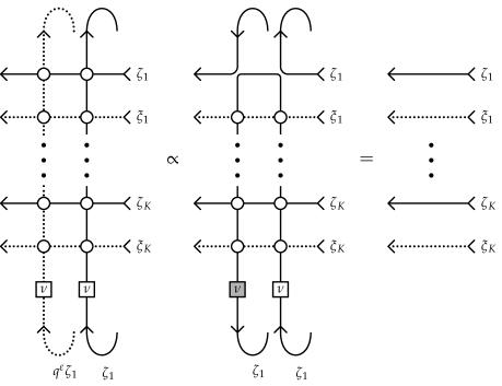
Successively applying the crossing relations 3.7, 3.7 and 3.23, the unitarity relations 3.9 and 3.14, the commutativity of the operators and , and the initial condition 3.16, we come to the middle picture. Here we acquire the scalar factor . Finally, using the unitarity relations 3.9 and 3.14, we get the right picture. Thus, we have the equation
| (4.1) |
or in terms of eigenvalues
Remembering now about the factor we acquired in transition from figure A.2 to figure A.8, we conclude that the comparison of these figures gives the equation
| (4.2) |
This equation, together with (4.2), can be used, in particular, for investigation of the correlation functions at finite non-zero temperature. However, the necessity to fix some spectral parameters leads to some problems and the additional work is required. Here we consider the zero temperature limit which is obtained as follows. We put and and take the limit , , keeping the ratio fixed and equal to . The resulting equation is
| (4.3) |
where
Certainly, in the case , , we have .
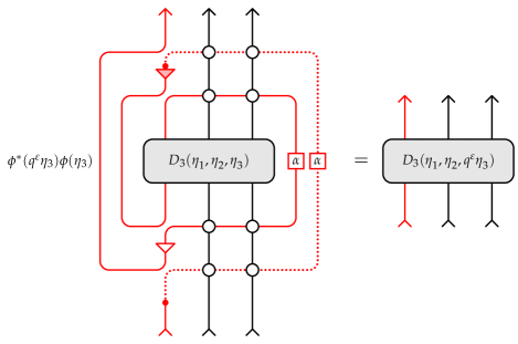
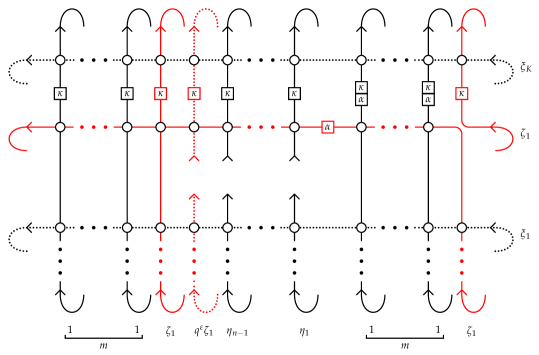
It is constructive to give the graphical image of equation (4.3). Below, using pictures, we assume that . It is enough to understand the general situation. It is clear that figure 4.2 depicts equation (4.3).
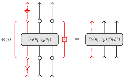
Fat dots in the picture means changing the interpretation of the type of line. Namely, an input line corresponding to a representation is treated as the output line corresponding to the dual representation and so on. Note that the order of the vector spaces is from the right to the left. Cut the red line above the box with the label in the left hand side of this equation and slightly deform the picture to obtain figure 4.4.
Remember that if is finite dimensional, the space of linear operators on can be identified with the space . To this end one defines the mapping by the equation
One can show that it is a bijective mapping. Using it, one defines the mapping from to which sends an operator to the operator
We numerate the vector spaces as . Now we can write the analytical expression for the figure 4.4. It is not difficult to generalize it to the case of an arbitrary . Now, taking the trace over the additional space, we come to the following analytical expression for the first equation
| (4.4) |
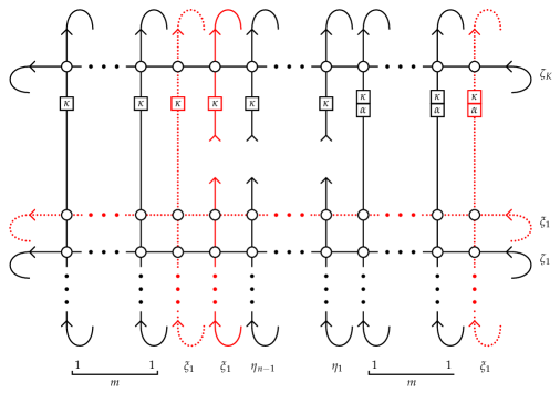
4.2. Second equation
The graphical proof of the second equation is very similar to the proof of the first one. The initial and the final points can be found in figures A.10 and A.10. If we take the operator depicted in figure A.10, divide it by , put and take the limit , we obtain the action of some linear operator on the operator . Applying this procedure to the operator of figure A.10, we come to the expression
In a similar way as for equation (4.1) we obtain
or in terms of eigenvalues
Using this relation, we see that the comparison of figures A.10 and A.10 leads to the equation
| (4.5) |
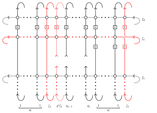
The zero temperature limit is obtained as follows. We put and and take the limit , , keeping the ratio fixed and equal to . The resulting equation is
| (4.6) |
where
In the case , , we have .
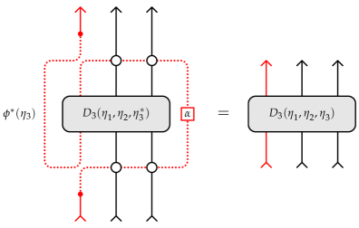
Cut the dotted red line in the left hand side of this equation above the box with the label and slightly deform the picture to obtain figure 4.4. Writing the analytical expression for the figure 4.4, generalizing to the case of an arbitrary , and taking the trace over the additional space, come to the following analytical expression for the second equation
| (4.7) |
4.3. Full rqKZ equation
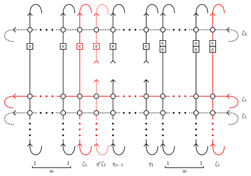
Combining equations (4.3) and (4.6), we come to the final reduced qKZ equation
The graphical image of this equation can be obtained by combining the graphical equations given in figures 4.2 and 4.5, see figure 4.6.
Now we have two additional spaces, and , and numerate the spaces as . Combining equations (4.4) and (4.7), we obtain the following full reduced qKZ equation
This is the main result of the present paper. In fact, we have the equation satisfied by the zero temperature correlation functions of the chain associated with the loop Lie algebra . To investigate correlation function at arbitrary temperature one should return to equations (4.2) and (4.5).
5. Conclusions
We have derived the reduced qKZ equation for the quantum integrable system related to an arbitrary quantum loop algebra. The main feature of the general case compared to the simplest -case is that the first fundamental representation does not coincide with its dual, and so, to obtain a closed form of the reduced qKZ equation, two successive steps are needed. We have demonstrated that all necessary unitarity and crossing relations follow from the properties of the algebra. The status of the initial condition is not completely clear. From one side, we do not see how it can be obtained from the properties of the algebra. From the other side, as we know, all -operators found in the framework of the quantum group approach satisfy this condition.
Our result refers to the zero temperature case. In fact, intermediate equations (4.2) and (4.5) can be used as a starting point to investigate the nonzero temperature case. The corresponding consideration for the quantum loop algebra can be found in paper [41]. It should be noted that in the general case some additional problems arise. We hope to return to this later.
Acknowledgments
We thank our colleagues and coauthors H. Boos and F. Göhmann for numerous fruitful discussions. KhSN was supported in part by the DFG grant # BO3401/31 and by the Russian Academic Excellence Project ‘5-100’. AVR thanks the Max Plank Institute for Mathematics in Bonn for the warm hospitality extended to him during the work on this paper. This work was also supported in part by the RFBR grant # 20-51-12005.
Appendix: Graphical derivation of rqKZ equation
A.1. First equation
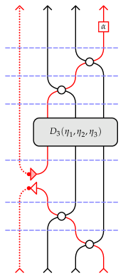
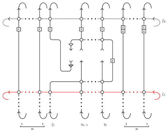
The initial configuration for the graphical derivation of the first part of the reduced qKZ equation is given in figure A.2. The figure represents the action of an operator, which we denote by , on . We mark by red the lines with the spectral parameter . The triangle and the filled triangle corresponding to the operator and its inverse are introduced to use further the crossing relations depicted in figures 3.7 and 3.7. We put , use the initial condition 3.16 and proceed to figure A.2.
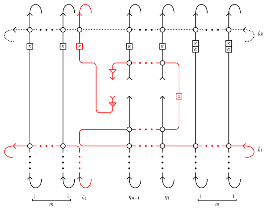
We pull off the emerging loop and raise the arising corner of the red line to the free corner above. This leads us to figure A.4.
We move the ‘swing seat’ down, then back up and front down again. To pass through horizontal lines we use the unitarity relations 3.9 and 3.14. After that we insert the product into the ‘swing seat’ and go to figure A.4.
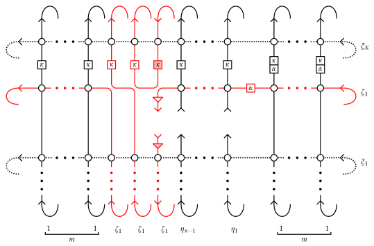
Now we restore all split vertices and, using the equations represented by figures 3.7, 3.7 and 3.23, and the unitarity relations given in figures 3.14 and 3.11, reverse the direction of the red vertical line which goes from top to bottom. The commutativity of the operators and is also used. We acquire the overall factor , where and is defined by equation (3.7). We keep this factor in mind. It is clear that the arising red dotted line is associated with the spectral parameter . After all that we come to figure A.6.
We move the leftmost red line behind the scene to the rightmost position, use the initial condition 3.16 and obtain the configuration given in figure A.6.
The next task is to find the right place for the red box with the label . We use iteratively the graphical equation given in figure 3.25 and proceed to the next figure.
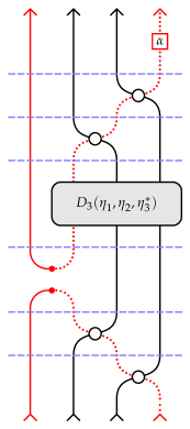
A.2. Second equation
The initial point of the graphical derivation of the second part of the reduced qKZ equation is given in figure A.10. Note that to apply the corresponding initial condition we make some rearrangement of the horizontal transfer operators using their commutativity. The figure represents the action of an operator, which we denote by , on the operator . Now we mark by red the lines with the spectral parameter . We put and perform transformations similar to those which we made in the derivation of the first part.
The final point of the graphical derivation of the second part of the reduced qKZ equation can be seen in figure A.10.


References
- [1] V. G. Drinfeld, Quantum groups, Proceedings of the International Congress of Mathematicians, Berkeley, 1986 (A. E. Gleason, ed.), vol. 1, American Mathematical Society, Providence, 1987, pp. 798–820.
- [2] M. Jimbo, A -difference analogue of and the Yang-Baxter equation, Lett. Math. Phys. 10 (1985), 63–69.
- [3] M. Jimbo, K. Miki, T. Miwa, and A. Nakayashiki, Correlation functions of the XXZ model for , Phys. Lett. A 168 (1992), 256.
- [4] M. Jimbo and T. Miwa, Quantum KZ equation with and correlation functions of the XXZ model in the gapless regime, J. Phys. A 29 (1996), 2923.
- [5] H. Boos, A. Hutsalyuk, and Kh. S. Nirov, On the calculation of the correlation functions of the -model by means of the reduced qKZ equation, J. Phys. A: Math. Theor. 51 (2018), 445202 (29pp), arXiv:1804.09756 [hep-th].
- [6] G. A. P. Ribeiro and A. Klümper, Correlation functions of the integrable spin chain, J. Stat. Mech.: Theor. Exp. (2019), 013103 (31pp), arXiv:1804.10169 [math-ph].
- [7] H. Boos, F. Göhmann, A. Klümper, Kh. S. Nirov, and A. V. Razumov, Universal -matrix and functional relations, Rev. Math. Phys. 26 (2014), 1430005 (66pp), arXiv:1205.1631 [math-ph].
- [8] V. V. Bazhanov, S. L. Lukyanov, and A. B. Zamolodchikov, Integrable structure of conformal field theory, quantum KdV theory and thermodynamic Bethe ansatz, Commun. Math. Phys. 177 (1996), 381–398, arXiv:hep-th/9412229.
- [9] V. V. Bazhanov, S. L. Lukyanov, and A. B. Zamolodchikov, Integrable structure of conformal field theory II. Q-operator and DDV equation, Commun. Math. Phys. 190 (1997), 247–278, arXiv:hep-th/9604044.
- [10] V. V. Bazhanov, S. L. Lukyanov, and A. B. Zamolodchikov, Integrable structure of conformal field theory III. The Yang–Baxter relation, Commun. Math. Phys. 200 (1999), 297–324, arXiv:hep-th/9805008.
- [11] S. M. Khoroshkin and V. N. Tolstoy, The uniqueness theorem for the universal -matrix, Lett. Math. Phys. 24 (1992), 231–244.
- [12] S. Levenderovskiĭ, Ya. Soibelman, and V. Stukopin, The quantum Weyl group and the universal quantum -matrix for affine Lie algebra , Lett. Math. Phys. 27 (1993), 253–264.
- [13] Y.-Z. Zhang and M. D. Gould, Quantum affine algebras and universal -matrix with spectral parameter, Lett. Math. Phys. 31 (1994), 101–110, arXiv:hep-th/9307007.
- [14] A. J. Bracken, M. D. Gould, Y.-Z. Zhang, and G. W. Delius, Infinite families of gauge-equivalent -matrices and gradations of quantized affine algebras, Int. J. Mod. Phys. B 8 (1994), 3679–3691, arXiv:hep-th/9310183.
- [15] A. J. Bracken, M. D. Gould, and Y.-Z. Zhang, Quantised affine algebras and parameter-dependent -matrices, Bull. Austral. Math. Soc. 51 (1995), 177–194.
- [16] H. Boos, F. Göhmann, A. Klümper, Kh. S. Nirov, and A. V. Razumov, Exercises with the universal -matrix, J. Phys. A: Math. Theor. 43 (2010), 415208 (35pp), arXiv:1004.5342 [math-ph].
- [17] H. Boos, F. Göhmann, A. Klümper, Kh. S. Nirov, and A. V. Razumov, On the universal -matrix for the Izergin–Korepin model, J. Phys. A: Math. Theor. 44 (2011), 355202 (25pp), arXiv:1104.5696 [math-ph].
- [18] V. V. Bazhanov and Z. Tsuboi, Baxter’s Q-operators for supersymmetric spin chains, Nucl. Phys. B 805 (2008), 451–516, arXiv:0805.4274 [hep-th].
- [19] H. Boos, F. Göhmann, A. Klümper, Kh. S. Nirov, and A. V. Razumov, Universal integrability objects, Theor. Math. Phys. 174 (2013), 21–39, arXiv:1205.4399 [math-ph].
- [20] A. V. Razumov, Monodromy operators for higher rank, J. Phys. A: Math. Theor. 46 (2013), 385201 (24pp), arXiv:1211.3590 [math.QA].
- [21] V. V. Bazhanov, A. N. Hibberd, and S. M. Khoroshkin, Integrable structure of conformal field theory, quantum Boussinesq theory and boundary affine Toda theory, Nucl. Phys. B 622 (2002), 475–574, arXiv:hep-th/0105177.
- [22] T. Kojima, Baxter’s -operator for the -algebra , J. Phys. A: Math. Theor 41 (2008), 355206 (16pp), arXiv:0803.3505 [nlin.SI].
- [23] H. Boos, F. Göhmann, A. Klümper, Kh. S. Nirov, and A. V. Razumov, Quantum groups and functional relations for higher rank, J. Phys. A: Math. Theor. 47 (2014), 275201 (47pp), arXiv:1312.2484 [math-ph].
- [24] Kh. S. Nirov and A. V. Razumov, Quantum groups and functional relations for lower rank, arXiv:1412.7342 [math-ph].
- [25] Kh. S. Nirov and A. V. Razumov, Vertex models and spin chains in formulas and pictures, arXiv:1811.09401 [math-ph].
- [26] I. B. Frenkel and N. Yu. Reshetikhin, Quantum affine algebras and holonomic difference equations, Commun. Math. Phys. 146 (1992), 1–60.
- [27] J.-P. Serre, Complex semisimple Lie algebras, Springer Monographs in Mathematics, Springer, Berlin, 2001.
- [28] J. E. Humphreys, Introduction to Lie algebras and representation theory, Springer, New York, 1980.
- [29] V. N. Tolstoy and S. M. Khoroshkin, The universal -matrix for quantum utwisted affine Lie algebras, Funct. Anal. Appl. 26 (1992), 69–71.
- [30] S. M. Khoroshkin and V. N. Tolstoy, On Drinfeld’s realization of quantum affine algebras, J. Geom. Phys. 11 (1993), 445–452.
- [31] S. Khoroshkin and V. N. Tolstoy, Twisting of quantum (super)algebras. Connection of Drinfeld’s and Cartan-Weyl realizations for quantum affine algebras, arXiv:hep-th/9404036.
- [32] J. Beck, Convex bases of PBW type for quantum affine algebras, Commun. Math. Phys. 165 (1994), 193–199, arXiv:hep-th/9407003.
- [33] I. Damiani, La -matrice pour les algèbres quantiques de type affine non tordu, Ann. Sci. École Norm. Sup. 31 (1998), 493–523.
- [34] T. Tanisaki, Killing forms, Harish-Chandra homomorphisms and universal -matrices for quantum algebras, Infinite Analysis (A. Tsuchiya, T. Eguchi, and M. Jimbo, eds.), Advanced Series in Mathematical Physics, vol. 16, World Scientific, Singapore, 1992, pp. 941–962.
- [35] P. Etingof, B. Frenkel, and A. A. Kirillov, Lectures on representation theory and Knizhnik–Zamolodchikov equations, Mathematical Surveys and Monographs, vol. 58, American Mathematical Society, Providence, 1998.
- [36] M. Suzuki, Transfer-matrix method and Monte Carlo simulation in quantum spin systems, Phys. Rev. B 31 (1985), 2957.
- [37] H. Boos, M. Jimbo, T. Miwa, F. Smirnov, and Y. Takeyama, Hidden Grassmann structure in the XXZ model, Commun. Math. Phys. 272 (2007), 263–281, arXiv:hep-th/0606280.
- [38] H. Boos, M. Jimbo, T. Miwa, F. Smirnov, and Y. Takeyama, Hidden Grassmann structure in the XXZ model II: Creation operators, Commun. Math. Phys. 286 (2009), 875–932, arXiv:0801.1176 [hep-th].
- [39] M. Jimbo, T.Miwa, and F. Smirnov, Hidden Grassmann structure in the XXZ model III: Introducing the Matsubara direction, J. Phys. A: Math. Theor. 42 (2009), 304018 (31pp), arXiv:0811.0439 [math-ph].
- [40] B. Aufgebauer, Berechnung der Korrelationsfunktionen des Heisenberg-Modells bei endlicher Temperatur mittels Funktionalgleichungen, Ph.D. thesis, Bergische Universität Wuppertal, 2011.
- [41] B. Aufgebauer and A. Klümper, Finite temperature correlation functions from discrete functional equations, J. Phys. A: Math. Theor. 45 (2012), 345203 (20pp), arXiv:1205.5702 [cond-math.stat-mech].