Geometric Algorithm of Schrödinger Flow on a Sphere

Abstract

We construct the solution to the periodic Cauchy problem of the Schrödinger flow on the sphere. Such construction of solutions is formulated explicitly and therefore a geometric algorithm of solving this periodic Cauchy problem follows. Theoretical and experimental results will be discussed.

14H70, 17B80, 53-04, 68U20

1 Introduction

The Schrödinger flow on the unit sphere $\mathbb{S}^{2}$ is given by

(1) $$\gamma_{t}=\gamma\times\gamma_{xx},$$

where $\gamma(x,t)$ is a real-valued vector function of $\mathbb{S}^{2}$ on $(x,t)\in{\mathbb{R}}\times[0,\infty)$, and $\times$ is the cross product in ${\mathbb{R}}^{3}$. We call $\gamma(x,t)$ satisfying (1) a Schrödinger curve. This curve evolution (1) corresponds to the non-linear Schrödinger equation (NLS)

(2) $$q_{t}=i(q_{xx}+2|q|^{2}q).$$

Takhtajan [9] first applied the inverse scattering method to describe its solution scheme. Tjon and Wright in [14] studied solitons of (1) in one dimension for the isotropic and anisotropic cases. The relation between (1) and (2) has been discussed by Terng and Uhlenbeck in [13], and by Zakharov and Takhtadzhyan in [15], where (1) is known as the isotropic Heisenberg ferromagnet.

It is well-known that (2) is relevant to the vortex filament equation (VFE) in ${\mathbb{R}}^{3}$ defined by

(3) $$\alpha_{t}=\alpha_{x}\times\alpha_{xx}.$$

This was first discovered by Da Rios in 1906 to model the movement of a thin vortex in a viscous fluid. In particular, (3) preserves the arc length parameter. So we may assume $||\alpha_{x}(x,t)||=1$ for all $t$, i.e., $\alpha(\cdot,t)$ is parametrized by its arc-length. Given a solution $\alpha(x,t)$ of VFE, Hasimoto ([3] ) relates (3) to (2) via the following transform

(4) $$q(x,t)=k(x,t)e^{i(\theta(t)+\int_{0}^{x}\tau(s,t)ds)},$$

where $k(\cdot,t),\tau(\cdot,t)$ are the curvature and torsion for $\alpha(\cdot,t)$, respectively, and $x$ is the arc-length parameter. Moreover, $q(x,t)$ is a solution of NLS. For example, a solution of the VFE $\alpha(x,t)=(\cos x,\sin x,t)$ with $k(x,t)=1,$ $\tau(x,t)=0$ corresponds to a solution of NLS $q(x,t)=e^{2it}$.

Numerical solutions of VFE have been studied for years. In 1998, Hou, Klapper, and Si provided a formulation in [4] for calculating solutions of VFE numerically. This method is a generalization of their 2-D work [5], in which they use the tangent angle ($\theta$) and arc length ($L$) method for planar curves. This $\theta-L$ formulation has none of high order time step stability constraints. Hou et al. then proposed to use the normal principal curvatures $k_{1},k_{2}$ as new variables to compute the motion of the curve in space.

If one differentiates a solution $\alpha(x,t)$ of (3) with respect to $x$, a Schrödinger curve is given by $\alpha_{x}$. In general, numerical solution of (1) can be obtained this way. Using geometry, Terng and Uhlenbeck in [10, 13] formulate the correspondences between NLS, VFE and Schrödinger flow on $\mathbb{S}^{2}$. In fact, they systematically construct solutions of such curve flows by making use of Lax pairs of NLS and Lie theory.

This construction of solutions to a geometric curve flow, if found, leads to a geometric algorithm to obtain numerical solutions to a curve flow. Namely, this approach gives rise to both analytic and numerical solutions of Schrödinger flow directly. One advantage of this geometric method is that we reduce curve PDEs, which are highly nonlinear, to integrable partial differential equations and ODE systems. As one of the most famous integrable PDEs, the NLS can be solved and computed numerically using various methods (for example, the pseudo spectral method, which provides a good accuracy for periodic solutions). There are several schemes that solve ODE systems well, such as ode solvers in Matlab and Runge-Kutta method.

Another advantage is that there are conservation properties since NLS is solitary. For instance, suppose $\gamma$ is a solution to (1). We now consider the energy structure. Let $\mathcal{E}(\gamma(t))=||\gamma_{x}(t)||^{2}_{L^{2}}$ be the energy function. Then the energy is conserved:

(5) $$\mathcal{E}(\gamma(t))=\mathcal{E}(\gamma(0)),$$

for any $t>0$. Besides, there are infinitely many conservation laws for NLS. Hence, one can verify the accuracy of the algorithm by analyzing these conserved quantities. Finally, this geometric algorithm can be implemented easily, even for beginners in programming.

The paper is organized as follows.

In Section 2, we recall the equivalence relations from results of Terng, Uhlenbeck and Thorbergsson. Proofs are given since they give rise to initial data in implementing. The essential idea works for both the Schrödinger flow and the VFE, although their constructions of formulations for curve solutions are different. We will focus on the Schrödinger flow on the unit sphere in the present article. In Section 3, we formulate the solution of the periodic Cauchy problem of (1) with an initial closed curve given. In Section 4, we give steps of our geometric algorithm, issues coming from implementing, error estimates for a stationary solution, and exhibit two explicit examples of periodic solutions with the viviani’s curve and spherical sinusoid as initial curves. In the end of this section, we also give one example of VFE that features the motion of smoke rings. The discussions about error estimates are in Section 5, and the conclusions follow in Section 6.

2 Equivalence of the Schrödinger flow on Hermitian symmetric spaces and the NLS

Suppose $(M,J,g,w)$ is a compact Kähler manifold with a complex structure $J$, the Riemannian metric $g$, and a symplectic form $w$ on $M$ satisfying $w(X,Y)=g(JX,Y)$. The Schrödinger flow on $M$ (cf. [11]) is the evolution equation on $C^{\infty}({\mathbb{R}},M)$:

(6) $$\gamma_{t}=J_{\gamma}(\nabla_{\gamma_{x}}\gamma_{x}),$$

where $\nabla$ is the Levi-Civita connection of the metric $g$. When $M={\mathbb{C}}^{n}$, (6) is the linear Schrödinger equation $\gamma_{t}=i\gamma_{xx}$. When $M=\mathbb{S}^{2}$, (6) gives us the Heisenberg ferromagnetic model for $\gamma:{\mathbb{R}}^{2}\rightarrow\mathbb{S}^{2}$. Indeed, the complex structure of $\mathbb{S}^{2}$ at $\gamma$ sends $v$ to $\gamma\times v$ on $T\mathbb{S}^{2}_{\gamma}$, where $\times$ is the cross product in ${\mathbb{R}}^{3}$. Then

(7) $$\gamma\times\nabla_{\gamma_{x}}\gamma_{x}=\gamma\times\gamma_{xx}^{T}=\gamma\times(\gamma_{xx}-(\gamma_{xx},\gamma)\gamma)=\gamma\times\gamma_{xx},$$

which obviously is the evolution (1) on $\mathbb{S}^{2}$.

The Schrödinger flow (6) is a Hamiltonian equation for the energy functional on $C^{\infty}(\mathbb{S}^{1},M)$ with respect to an induced symplectic form by $\omega$ on $C^{\infty}(\mathbb{S}^{1},M)$ ([11]). Note that the critical points of the energy functional are geodesics of $(M,g)$, so the stationary solutions of the Schrödinger flow on $M$ are closed geodesics of $M$. Furthermore, if $M$ is a Hermitian symmetric space, then (6) can be written in terms of the Lie bracket.

To be more precise, let $G$ be a simple complex Lie group, and $\tau$ the involution that gives the maximal compact subgroup $U$. It is known that there exists $a\in{\mathcal{U}}$ such that ${\rm ad}(a)^{2}|_{{\mathcal{P}}}=-{\rm Id\/}_{{\mathcal{P}}}$ and ${\mathcal{U}}={\mathcal{K}}\oplus{\mathcal{P}}$, where ${\mathcal{K}}$ is the centralizer of $a$ in ${\mathcal{U}}$ and ${\mathcal{P}}$ is the orthogonal complement of ${\mathcal{K}}$. Then the Adjoint $U$-orbit at $a$ in ${\mathcal{U}}$ is diffeomorphic to $U$ and is a compact irreducible Hermitian $\frac{U}{K}$ symmetric space.

We briefly review some results on the Schrödinger flow proved by Terng and Uhlenbeck in [13] for $\frac{U}{K}={\rm Gr}(k,{\mathbb{C}}^{n})$ and by Terng and Thorbergsson in [11] for the other three classical Hermitian symmetric spaces.

Proposition 2.1 ([11],[13]).

Under the embedding of the Hermitian symmetric space $\frac{U}{K}$ as the Adjoint orbit $U\cdot a$ in ${\mathcal{U}}$, the Schrödinger flow on $\frac{U}{K}$ is

(8) $$\gamma_{t}=[\gamma,\gamma_{xx}].$$

A Lax pair for (8) is also derived and proved to be gauge equivalent to a Lax pair of NLS by Terng and Uhlenbeck [13]. Proposition 2.1 implies that if $M$ is a Hermitian symmetric space, then two evolutions, (6) and (8) are equivalent. In particular, we have $\gamma_{t}=[\gamma,\gamma_{xx}]=\gamma\times\gamma_{xx}$ for $M=\mathbb{S}^{2}$.

Theorem 2.2 and Theorem 2.4 show the construction of NLS solutions from solutions of the Schrödinger flow and vice versa. We give a proof since the approach will be used later in coding.

Theorem 2.2 ([11],[12]).

Let $\gamma:{\mathbb{R}}^{2}\to\frac{U}{K}$ be a solution of the Schrödinger flow on the Hermitian symmetric space $\frac{U}{K}=U\cdot a\subset{\mathcal{U}}$. Then there exists $g:{\mathbb{R}}^{2}\to U$ satisfying

1. $\gamma=gag^{-1}$,

2. $u=g^{-1}g_{x}:{\mathbb{R}}^{2}\to{\mathcal{U}}_{a}^{\bot}$ satisfies the $\frac{U}{K}$-NLS equation:

   (9) $$u_{t}=[a,u_{xx}]-\frac{1}{2}[u,[u,[a,u]]],$$

3. $g^{-1}g_{t}=[a,u_{x}]-\frac{1}{2}[u,[a,u]]$.

Moreover, $\tilde{g}$ satisfies (i) and (ii) if and only if there is a constant $C\in U_{a}$ such that $\tilde{g}=gC.$

Proof 2.3.

We recall that $K=U_{a},P=U_{a}^{\bot}$ and ${\mathcal{U}}={\mathcal{K}}\oplus{\mathcal{P}}$. Suppose $\gamma(x,t)$ is a solution of (8). Then there exists $h:{\mathbb{R}}^{2}\to U$ such that $\gamma(x,t)=h(x,t)ah(x,t)^{-1}$. Let $\pi_{0},\pi_{1}$ be orthogonal projections of ${\mathcal{U}}$ onto ${\mathcal{K}},{\mathcal{P}}$, respectively. We choose $k:{\mathbb{R}}^{2}\to K$ such that $k_{x}k^{-1}=-\pi_{0}(h^{-1}h_{x})$. Set $f(x,t)=h(x,t)k(x,t)$, then $\gamma=faf^{-1}$. Moreover,

(10) $$f^{-1}f_{x}=(hk)^{-1}(hk)_{x}=k^{-1}\pi_{1}(h^{-1}h_{x})k\in{\mathcal{P}}.$$

A direct computation shows that

$$\gamma_{x}=f[f^{-1}f_{x},a]f^{-1}=f[u,a]f^{-1}\mbox{ and }[\gamma,\gamma_{x}]=fuf^{-1}.$$

Since $\tau_{\lambda}=\gamma\lambda dx+(\gamma\lambda^{2}+[\gamma,\gamma_{x}]\lambda)dt$ is flat for all $\lambda\in{\mathbb{C}}$, $f*\tau_{\lambda}$ is flat, i.e. the following connection is flat for all $\lambda\in{\mathbb{C}}$:

(11) $$f^{-1}\tau_{\lambda}f+f^{-1}df=(a\lambda+u)dx+(a\lambda^{2}+u\lambda+f^{-1}f_{t})dt.$$

Therefore, $(a\lambda^{2}+u\lambda+f^{-1}f_{t})_{x}-(a\lambda+u)_{t}+[a\lambda+u,f^{-1}f_{t}]=0$.

(12) $$u_{x}+[a,f^{-1}f_{t}]=0$$

(13) $$(f^{-1}f_{t})_{x}-u_{t}+[u,f^{-1}f_{t}]=0.$$

Write

$$f^{-1}f_{t}=P+T,$$

where $P\in{\mathcal{P}}$ and $T\in{\mathcal{K}}$, respectively. From (12), we have

(14) $$P=[a,u_{x}],~{}T_{x}=-\frac{1}{2}[u,[a,u]]_{x}.$$

So, $T=-\frac{1}{2}[u,[a,u]]+c(t)$ for some function $c(t)$.

Define $g=fy(t)$, where $y(t)\in{\mathcal{K}}$ such that $y_{t}y^{-1}=-c(t).$

Next, we will show that $g$ defined above satisfies the conditions $(i)-(iii)$. Since $y(t)$ and $a$ commute, it is easy to see that $gag^{-1}=\gamma$. In particular,

(15) $$g^{-1}g_{x}=y^{-1}f^{-1}f_{x}y=y^{-1}uy\in{\mathcal{P}},$$

(16) $$g^{-1}g_{t}=y^{-1}(f^{-1}f_{t}+y_{t}y^{-1})y=-\frac{1}{2}[y^{-1}uy,[a,y^{-1}uy]],$$

which means $y^{-1}uy$ is a solution of (9).

For the uniqueness, suppose $\tilde{g}$ satisfies $(1)-(2)$, and set $C=g^{-1}\tilde{g}$. Then

(17) $$\tilde{g}^{-1}\tilde{g}_{x}=C^{-1}g^{-1}g_{x}C+C^{-1}C_{x}.$$

Since $\tilde{g}^{-1}\tilde{g}_{x}$ and $C^{-1}g^{-1}g_{x}C$ are in ${\mathcal{P}}$ while $C^{-1}C_{x}\in{\mathcal{K}}$,

(18) $$C^{-1}C_{x}=0.$$

Similarly, $C^{-1}C_{t}=0$. So $C$ is constant.

The converse is also true.

Theorem 2.4 ([11], [12]).

Let $u:{\mathbb{R}}^{2}\to{\mathcal{U}}_{a}^{\bot}$ be a smooth solution of (9). Then given any $c_{0}\in U$, the following linear system for $g:{\mathbb{R}}^{2}\to U$,

(19) $$\begin{cases}g^{-1}g_{x}=u,\\ g^{-1}g_{t}=[a,u_{x}]-\frac{1}{2}[u,[a,u]],\\ g(0,0)=c_{0}\end{cases}$$

has a unique smooth solution $g:{\mathbb{R}}^{2}\to U$. Moreover, $\gamma(x,t)=g(x,t)ag(x,t)^{-1}$ is a solution of the Schrödinger flow (8) on $\frac{U}{K}$.

In fact, when $\lambda=\lambda_{0}$ is any arbitrary real number, a shift of $\gamma=gag^{-1}$ by $2\lambda_{0}$ is also a solution of (8).

Proposition 2.5.

Let $u:{\mathbb{R}}^{2}\to{\mathcal{U}}_{a}^{\bot}$ be a solution of (9) and $E$ satisfy

(20) $$\begin{cases}E^{-1}E_{x}=a\lambda+u,\\ E^{-1}E_{t}=a\lambda^{2}+u\lambda+[a,u_{x}]-\frac{1}{2}[u,[a,u]].\end{cases}$$

If $\lambda_{0}\in{\mathbb{R}}$ and $g(x,t)=E(x,t,\lambda_{0})$, then $\gamma=gag^{-1}(x-2\lambda_{0}t,t)$ is a solution of (8).

Proof 2.6.

Let $\eta(x,t)=gag^{-1}(x,t)$ and denote $Q_{-1}=[a,u_{x}]-\frac{1}{2}[u,[a,u]]$. It can be checked that

(21) $$\begin{array}[]{l}\eta_{x}=g[u,a]g^{-1},\\ \eta_{t}=g[u\lambda_{0}+Q_{-1},a]g^{-1}.\end{array}$$

Direct computations show that

(22) $$\gamma_{xx}=g[a\lambda_{0}+u,[u,a]]g^{-1}+g[u_{x},a]g^{-1},$$

and therefore we obtain

(23) $$\gamma\times\gamma_{xx}=g[a,u\lambda_{0}]g^{-1}+gu_{x}g^{-1}.$$

We see that $\gamma_{t}=-2\lambda_{0}\eta_{x}+\eta_{t}$, which gives

(24) $$g[-u\lambda_{0},a]g^{-1}+g[Q_{-1},a]g^{-1}.$$

Here, since $[Q_{-1},a]=u_{x}$, $\gamma_{t}=[\gamma,\gamma_{xx}].$

We say $E$ is a frame of solution $u$ if $E$ is a solution of the ODE system (20).

Remark 2.7.

Consider $\gamma(x,t)$ to be a great circle on the unit sphere, i.e., $\gamma(x,t)=(\cos x,\sin x,0)$. It is obviously a solution to (8). Following from the proof of Theorem 2.2, one local invariant $q(x,t)$ is given by

(25) $$q(x,t)=\frac{i}{2}e^{\frac{i}{2}t},$$

that of course can be checked to solve the NLS.

Soliton solutions of the Schrödinger equation have been widely studied in history. One can compute soliton solutions using explicit formulations that are known. In fact, Bäcklund transformation gives $N$-soliton solutions for integrable systems, especially for the NLS. For example, [7] says the following:

Theorem 2.8.

(Bäcklund transformation) Let $E(x,t,\lambda)$ be a frame of a solution $u$ of the NLS (2), $\alpha\in{\mathbb{C}}\setminus{\mathbb{R}}$, and $\pi$ a Hermitian projection of ${\mathbb{C}}^{2}$ onto $V$. Define

(26) $$k_{\alpha,\pi}(\lambda)={\rm I\/}_{n}+\frac{\alpha-\bar{\alpha}}{\lambda-\alpha}\pi^{\perp}.$$

Let $\tilde{\pi}(x,t)$ be the Hermitian projection of ${\mathbb{C}}^{2}$ onto $\tilde{V}(x,t)=E(x,t,\alpha)^{-1}V$. Then we have

(27) $$\tilde{u}=u+(\alpha-\bar{\alpha})[a,\tilde{\pi}]$$

is a solution of the NLS and

(28) $$\tilde{E}(x,t,\lambda)=k_{\alpha,\pi}(\lambda)E(x,t,\lambda)k^{-1}_{\alpha,\tilde{\pi}(x,t)}$$

is a frame of $\tilde{u}$.

3 Main results

The correspondence discussed in Theorem 2.2 and Theorem 2.4 gives a systematic way to construct solution of the Schrödinger flow, and hence the initial value problem of the Schrödinger flow can be solved. In this section, we focus on the sphere case, in particular, we consider the periodic Cauchy problem. Namely, given a closed curve $\gamma_{0}(x)$ on a unit sphere, we show the existence of a $L$-periodic curve that evolves according to the Schrödinger flow Eq. 1 and write down the algebraic solution formula explicitly. Without loss of generality, we assume the period $L$ is $2\pi$ for the rest of article. The main theorem is the following.

Theorem 3.1.

Given a smooth closed curve $\gamma_{0}(x):[0,2\pi]\rightarrow\mathbb{S}^{2}$ with period $2\pi$. Then there exists a unique $x$-periodic $\gamma(x,t)$ with period $2\pi$ satisfying

(29) $$\left\{\begin{array}[]{rcl}\gamma_{t}&=&\gamma\times\gamma_{xx}\\ \gamma(x,0)&=&\gamma_{0}(x)\end{array}\right..$$

We first note that Theorem 3.1 is a special case of the following Theorems 2.2 and 2.4. Theroem 2.2 shows that, for any arbitrary $\gamma_{0}(x):[0,2\pi]\to\mathbb{S}^{2}$ given, there is a frame $f:{\mathbb{R}}\to SU(2)$ such that $\gamma_{0}=faf^{-1}$, where $a={\rm diag}(\frac{i}{2},-\frac{i}{2})$, satisfying $f(0)=I_{2}$ and $f^{-1}f_{x}=u_{0}$, where $u_{0}$ is of the form

(30) $$u_{0}=\left(\begin{array}[]{cc}0&q_{0}\\ -\bar{q_{0}}&0\end{array}\right).$$

We notice that $f(x)$ found may not be periodic, so the essential idea is to find a periodic one. Below we show how to construct a periodic frame of $\gamma_{0}$.

Since $\gamma_{0}$ is periodic, $\gamma_{0}(2\pi)=\gamma_{0}(0)$. It yields that $f(2\pi)a=af(2\pi).$ That is, $f(2\pi)$ lies in the centralizer $SU(2)_{a}=\{{\rm diag}(e^{{\rm i\,}\theta},e^{-{\rm i\,}\theta})\ |\ \theta\in[0,2\pi)\}$ and hence we may write

(31) $$f(2\pi)=e^{2\pi c_{0}a},$$

for some constant $c_{0}$. A direct computation gives the following proposition.

Proposition 3.2.

Define

(32) $$\tilde{f}(x)=f(x)e^{-c_{0}ax}.$$

Then $\tilde{f}(x)$ has the following properties:

1. $\gamma_{0}=\tilde{f}a\tilde{f}^{-1}$

2. $\tilde{f}(x)$ is periodic in $x$

3. $\tilde{f}^{-1}\tilde{f}_{x}=\left(\begin{array}[]{cc}-\frac{i}{2}c_{0}&\tilde{q_{0}}\\ -\bar{\tilde{q_{0}}}&\frac{i}{2}c_{0}\end{array}\right)$, where $\tilde{q_{0}}(x)=q_{0}(x)e^{ic_{0}x}.$

4. $\tilde{q_{0}}$ is periodic.

Proposition 3.2 gives us a way to decompose the periodic curve $\gamma_{0}$ in terms of a periodic frame $\tilde{f}(x)$ and a local invariant $\tilde{q}_{0}(x)$. Here, we call $c_{0}$ the normal holonormy. Next, we evolve the curve according to the partial differential equation

(33) $$\gamma_{t}=\gamma\times\gamma_{xx}.$$

Proposition 3.3.

Suppose $\gamma(x,t):[0,2\pi]\to\mathbb{S}^{2}$ solves (33) and is periodic in $x$ with periodic $2\pi$. By Theorem 2.2, there exists $f:{\mathbb{R}}^{2}\to SU(2)$ such that $\gamma=faf^{-1}$, $f^{-1}f_{x}=u$, and $f^{-1}f_{t}=Q_{-1}$, where

(34) $$a={\rm diag}(\frac{i}{2},-\frac{i}{2}),\quad u=\begin{pmatrix}0&q\\ -\bar{q}&0\end{pmatrix},\quad Q_{-1}=\frac{i}{2}\begin{pmatrix}-|q|^{2}&q_{x}\\ \bar{q}_{x}&|q|^{2}\end{pmatrix}.$$

Define $c_{0}(t)$ to be a function of $t$ satisfying

(35) $$f^{-1}(0,t)f(2\pi,t)=e^{2\pi c_{0}(t)a}.$$

Then $c_{0}(t)$ is independent of $t$.

Proof 3.4.

Taking $t$-derivative of (35) gives

$$e^{2\pi c_{0}(t)a}2\pi c_{0}^{\prime}(t)a =-f^{-1}(0,t)f_{t}(0,t)f(2\pi,t)+f^{-1}(0,t)f_{t}(2\pi,t)$$

$$=e^{2\pi c_{0}(t)a}Q_{-1}(2\pi,t)-Q_{-1}(0,t)e^{2\pi c_{0}(t)a}.$$

It is easy to see that

(36) $$2\pi c_{0}^{\prime}(t)a=Q_{-1}(2\pi,t)-e^{-2\pi c_{0}(t)a}Q_{-1}(0,t)e^{2\pi c_{0}(t)a}.$$

A direct computation shows

(37) $$e^{-2\pi c_{0}(t)a}Q_{-1}(0,t)e^{2\pi c_{0}(t)a}=\frac{i}{2}\begin{pmatrix}-|q|^{2}&q_{x}e^{-4\pi ic_{0}(t)}\\ \bar{q}_{x}e^{4\pi ic_{0}(t)}&|q|^{2}\end{pmatrix}.$$

Note that $Q_{-1}(0,t)=Q_{-1}(2\pi,t)$. So, $c_{0}^{\prime}(t)=0,$ as desired.

Next, we consider the periodic Cauchy problem for NLS. Suppose that $q:{\mathbb{R}}^{2}\to{\mathbb{C}}$ is a solution of

(38) $$\left\{\begin{array}[]{ccl}q_{t}&=&i(q_{xx}+2|q|^{2}q)\\ q(x,0)&=&\tilde{q_{0}}(x).\end{array}\right.,$$

Let $E$ satisfy

(39) $$\begin{cases}E^{-1}E_{x}=\begin{pmatrix}\frac{i}{2}\lambda&q\\ -\bar{q}&-\frac{i}{2}\lambda\end{pmatrix},\\ E^{-1}E_{t}=\begin{pmatrix}\frac{i}{2}\lambda^{2}-i|q|^{2}&q\lambda+iq_{x}\\ -\bar{q}\lambda+i\bar{q}_{x}&-\frac{i}{2}\lambda^{2}+i|q|^{2}\end{pmatrix},\\ E(0,0,\bar{\lambda})^{*}=E(0,0,\lambda)^{-1}.\end{cases}$$

Then it turns out that there is a periodic frame for a solution $q$ of NLS periodic in $x$ in the following proof.

Proof 3.5 (Proof of Theorem 3.1).

Without loss of generality, we assume $\gamma_{0}(0)=a$. We know that there is $f\in SU(2)$ such that $\gamma_{0}=faf^{-1}$ and

(40) $$f^{-1}f_{x}=\begin{pmatrix}0&q_{0}\\ -\bar{q}_{0}&0\end{pmatrix}.$$

Since $\gamma_{0}$ is periodic, $f(2\pi)$ commutes with $a$. So $f(2\pi)=e^{2\pi c_{0}a}$ for some $c_{0}\in{\mathbb{R}}.$ Define

(41) $$\tilde{f}(x)=f(x)e^{-c_{0}ax}.$$

By Proposition 3.2, $\tilde{f}$ is periodic and $\gamma_{0}=\tilde{f}a\tilde{f}^{-1}$. In particular,

(42) $$\tilde{f}^{-1}\tilde{f}_{x}=\begin{pmatrix}-\frac{i}{2}c_{0}&q_{0}(x)e^{ic_{0}x}\\ -\bar{q}_{0}(x)e^{-ic_{0}x}&\frac{i}{2}c_{0}\end{pmatrix}.$$

Let $q(x,t)$ be the solution of

(43) $$\left\{\begin{array}[]{ccl}q_{t}&=&i(q_{xx}+2|q|^{2}q)\\ q(x,0)&=&q_{0}(x)e^{ic_{0}x}\end{array}\right.,$$

periodic in $x$, and $E(x,t,\lambda)$ the extended frame for $q$ satisfying

(44) $$\begin{cases}E^{-1}E_{x}=a(-c_{0})+u,\\ E^{-1}E_{t}=ac_{0}^{2}+u(-c_{0})+Q_{-1}(u),\\ E(0,0,-c_{0})=\tilde{f}(0).\end{cases}$$

We claim that $g(x,t)=E(x,t,-c_{0})$ is periodic in $x$ with period $2\pi$. Let $y(t)=g(2\pi,t)-g(0,t)$. We know $g^{-1}g_{t}=c_{0}^{2}a-c_{0}u+Q_{-1}(u)$ and $u=\begin{pmatrix}0&q\\ -\bar{q}&0\end{pmatrix}$ is periodic. Then

$$y^{\prime}(t) =g(2\pi,t)(c_{0}^{2}a-c_{0}u+Q_{-1}(u))|_{x=2\pi}-g(0,t)(c_{0}^{2}a-c_{0}u+Q_{-1}(u))|_{x=0}$$

$$=(g(2\pi,t)-g(0,t))(c_{0}^{2}a-c_{0}u+Q_{-1}(u))|_{x=0}$$

$$=y(t)A(t),$$

where $A(t)=(c_{0}^{2}a-c_{0}u+Q_{-1}(u))|_{x=0}.$

Since $y(0)=0$ solves the ODE $y^{\prime}(t)=y(t)A(t)$, the uniqueness theorem of ODE shows that $y(t)\equiv 0$. The claim follows. Let $\eta=gag^{-1}$. Then $\gamma(x,t)=\eta(x+2c_{0}t,t)$ is a solution of $\gamma_{t}=\gamma\times\gamma_{xx}$ by Proposition 2.5.

It remains to verify the initial condition. Note that Proposition 3.2 implies

(45) $$\gamma(x,0)=\eta(x,0)=\tilde{f}(x)a\tilde{f}^{-1}(x)=\gamma_{0}(x).$$

In particular, that $\gamma$ is periodic in $x$ follows from the periodicity of $E(x,t,-c_{0})$. Finally, the uniqueness of $\gamma$ follows from the uniqueness of $E(x,t,-c_{0})$.

4 Algorithm and Experimental results

Our analysis leads to the following algorithm to solve numerically the periodic Cauchy problem (3.1) with initial data $\gamma_{0}(x):[0,2\pi]\to\mathbb{S}^{2}$ being a closed initial curve on $\mathbb{S}^{2}$. In summary, the programming steps are as follows.

1. We first write $\gamma_{0}$ as an element in $\mathfrak{su}(2)$ and diagonalize $\gamma_{0}$ to find $f\in SU(2)$ such that $\gamma_{0}=faf^{-1}$ and

   $$f^{-1}f_{x}=\begin{pmatrix}0&q_{0}\\ -\bar{q}_{0}&0\end{pmatrix}.$$

2. Then compute $c_{0}$ by solving $f^{-1}(0)f(2\pi)=e^{2\pi c_{0}a}$.

3. We use the WGMS method in [8] (implicit spectral method) to solve the periodic Cauchy problem of NLS (38) with the initial data $q_{0}(x)e^{ic_{0}x}.$

4. compute $E$ by solving the ODE system (44) with the right hand side given by solutions $q$ of (38) and the initial data $fe^{-c_{0}ax}$.

5. calculate $\gamma=EaE^{-1}$ in terms of elements in $\mathfrak{su}(2)$ and then we map them back to ${\mathbb{R}}^{3}$, which is the numerical solution to (3.1).

Next, we compute the normal holonormy $c_{0}$, which gives the initial periodic data $q_{0}(x)e^{ic_{0}x}$ for the periodic Cauchy problem of NLS. The pseudo-spectral method [8] provides the numerical periodic solution to NLS with great accuracy.

With such numerical local invariant $q$ fitting in the right hand side of (39), we solve (39) using the Runge-Kutta method. Once $E$ is obtained, we calculate $\gamma=EaE^{-1}$ in terms of elements in $\mathfrak{su}(2)$ and then we map them back to ${\mathbb{R}}^{3}$. By Proposition 2.5 and the interpolation, the numerical solution to (3.1) is derived.

4.1 Experimental issues

The first step can be done simply by diagonalizing $f$. One can easily check that the diagonal entries are $0.5i$ and $-0.5i$, however, the function eig$(\cdot)$ in Matlab does not work well here. On one hand, the analytic $f$ in Step $1$ is a function that satisfies $\gamma_{0}(x)=f(x)af(x)^{-1}$ at each point $x$. On the other hand, we plug grid points $x_{i}$’s into $\gamma_{0}(x)$ before applying the eig in Matlab. This makes the eig function treat $\gamma_{0}(x_{i})$’s as individual scalar matrices, and then returns eigenvectors of $\gamma_{0}(x_{i})$ that don’t obey the same function since matrices formed by eigenvectors are not unique. For this reason, we need another way to figure out the $f$.

Identifying ${\mathbb{R}}^{3}$ with the skew-Hermitian matrices $\mathfrak{su}(2)$, we see that $\mathfrak{su}(2)$ has a standard basis consisting of the four elements

(46) $$a=\begin{pmatrix}\frac{i}{2}&0\\ 0&-\frac{i}{2}\end{pmatrix},b=\begin{pmatrix}0&\frac{1}{2}\\ -\frac{1}{2}&0\end{pmatrix},\mbox{ and }c=\begin{pmatrix}0&\frac{i}{2}\\ \frac{i}{2}&0\end{pmatrix},$$

and the map between elements in $\mathfrak{su}(2)$ and vectors $\gamma_{0}=(r_{1},r_{2},r_{3})$ on the sphere is

(47) $$\gamma_{0}=(r_{1},r_{2},r_{3})\mapsto r_{1}a+r_{2}b+r_{3}c=\begin{pmatrix}\frac{i}{2}r_{1}&\frac{1}{2}r_{2}+\frac{i}{2}r_{3}\\ -\frac{1}{2}r_{2}+\frac{i}{2}r_{3}&-\frac{i}{2}r_{1}\end{pmatrix},$$

denoted by $\Gamma_{0}$. A standard calculation of eigenvectors for $\Gamma_{0}$ shows

(48) $$F=\begin{pmatrix}\sqrt{\frac{1+r_{1}}{2}}&\frac{i}{\sqrt{2}}\frac{r_{2}+ir_{3}}{\sqrt{1+r_{1}}}\\ \frac{i}{\sqrt{2}}\frac{r_{2}-ir_{3}}{\sqrt{1+r_{1}}}&\sqrt{\frac{1+r_{1}}{2}}\end{pmatrix}$$

It can be checked that $F\in SU(2)$ and such $F$ is not unique. We make such choice of $F$ for the following reasons. When $r_{1}=1$, $r_{2}$ and $r_{3}$ are obviously zero, i.e., $\Gamma_{0}(1)=a$. This immediately implies the matrix of eigenvectors is the $2\times 2$ identity matrix, which agrees with our formulation of $F$. However, when $r_{1}=-1$, $\Gamma_{0}(-1)=-a$. The eigenvectors are

(49) $$\begin{pmatrix}0&i\\ i&0\end{pmatrix}.$$

Besides, let $r_{1}\rightarrow-1$, we have

(50) $$\frac{r_{2}+ir_{3}}{\sqrt{1+r_{1}}}\rightarrow\sqrt{2}e^{i\theta},\quad\theta=\tan\frac{r_{3}}{r_{2}}.$$

The limit of $F$ does not exist as $r_{1}\rightarrow-1$, and hence, this formulation is not continuous at $r_{1}=-1$. Without loss of generality, let $\gamma_{0}$ not pass through the point $(-1,0,0)$.

We also notice that $F^{-1}F_{x}$ might not be off-diagonal matrix. In order to make this happen, we follow Theorem Theorem 2.2 to rotate $F$ by a matrix $K$ where $-K_{x}K^{-1}$ is equal to the diagonal terms of $F^{-1}F_{x}$. For instance, consider $\gamma_{0}(x)=(0,\cos x,\sin x)$, then

(51) $$F(x)=\begin{pmatrix}\frac{1}{\sqrt{2}}e^{\frac{i}{2}x}&\frac{i}{\sqrt{2}}e^{\frac{i}{2}x}\\ \frac{i}{\sqrt{2}}e^{-\frac{i}{2}x}&\frac{1}{\sqrt{2}}e^{-\frac{i}{2}x}\end{pmatrix},\quad F^{-1}F_{x}=\begin{pmatrix}0&-\frac{1}{2}\\ \frac{1}{2}&0\end{pmatrix}.$$

4.2 Experimental errors

While actually implementing, the errors are provided to verify the accuracy of this geometric scheme. We would also like to see if numerical solutions obtained from our geometric algorithm preserve these relevant quantities. A fixed point $\gamma=a$ is the trivial solution of (1) with the local invariant $q=0$. Our implement immediately shows a fixed point on the sphere if we start with $\gamma_{0}(x)=(1,0,0)$. Given the initial curve to be a circle, then the exact solution is stationary, i.e.,

(52) $$\gamma(x,t)=(0,\cos x,\sin x).$$

The corresponding invariant is $q(x,t)=-\frac{1}{2}e^{\frac{i}{2}t}$, a solution of NLS. The following errors are estimated between the numerical solution $\gamma_{num}(x,t)$ and $\gamma(x,t)$ by the $L^{2}$-norm at each time $t$:

(53) $$E_{N}(t)=\left(\int_{0}^{2\pi}|\gamma_{num}(x,t)-\gamma(x,t)|^{2}~{}dx\right)^{\frac{1}{2}},$$

where $N$ indicates the number of $x$ partitions.

Table 1: $\triangle t=0.001$

$t$
steps	$E_{64}(t)$	$E_{128}(t)$	$E_{256}(t)$	$E_{512}(t)$
10	1.0851962E-02	2.722708E-03	6.84783037E-04	1.72447709E-04
20	1.0257888E-02	2.582122E-03	6.51822917E-04	1.58102531E-04
30	9.711601E-03	2.454641E-03	6.14796552E-04	1.34178170E-04
40	9.220668E-03	2.338847E-03	5.70308441E-04	1.19274466E-04
50	8.79326E-03	2.234083E-03	5.19933864E-04	1.16633012E-04
60	8.43756E-03	2.140637E-03	4.72659359E-04	1.19427212E-04
70	8.160922E-03	2.059924E-03	4.47994913E-04	1.44297698E-04
80	7.968884E-03	1.994621E-03	4.59273153E-04	1.93683390E-04
90	7.864274E-03	1.94872E-03	4.94939577E-04	2.49089493E-04
100	7.846684E-03	1.9274E-03	5.43976410E-04	3.11981115E-04

We also consider the maximal difference between $\gamma_{num}(x,t)$ and $\gamma(x,t)$ at each time $t$ given by

(54) $$E_{N}^{sup}(t)=max_{x\in I}\left(\|\gamma_{num}(x,t)-\gamma(x,t)\|\right),$$

where $I=\{j\frac{2\pi}{N}|j=0,1,2,\cdots,N-1\}.$

Table 2: $\triangle t=0.001$

$t$
steps	$E^{sup}_{64}(t)$	$E^{sup}_{128}(t)$	$E^{sup}_{256}(t)$	$E^{sup}_{512}(t)$
10	2.50304072E-04	8.83938616E-05	3.87637202E-05	1.59494744E-05
20	4.10069784E-04	1.60699569E-04	6.49229140E-05	1.97234863E-05
30	5.69783116E-04	2.22613774E-04	7.95435964E-05	1.68690680E-05
40	7.26480096E-04	2.74553194E-04	8.42922932E-05	2.76624306E-05
50	8.79882976E-04	3.17302096E-04	8.29884807E-05	4.21233398E-05
60	1.03000937E-03	3.51880564E-04	8.41160665E-05	5.42705369E-05
70	1.17668715E-03	3.79578845E-04	1.00586167E-04	7.04118124E-05
80	1.31944921E-03	4.02029934E-04	1.32082869E-04	9.19189874E-05
90	1.45756158E-03	4.21296895E-04	1.64970296E-04	1.13954497E-04
100	1.59011707E-03	4.39944903E-04	1.95175345E-04	1.37739549E-04

It is obvious that at a fixed time, the errors $E_{N}(t)$ and $E_{N}^{sup}(t)$ are decreasing when $N$ becomes bigger. Similarly, it is natural for us to consider how $E_{N}(t)$ behaves in time when $N$ is fixed. In Table 3, we demonstrate the global errors for different sizes of time steps. Namely,

(55) $$G_{N}^{sup}=max_{0\leq t_{n}\leq T}\left(E_{N}^{sup}(t_{n})\right),$$

where $T$ is the total time period.

Table 3: The error $G_{N}^{sup}$ computed for different $\triangle t$ with $T=1$

$N$	$\triangle t=\frac{1}{200}$	$\triangle t=\frac{1}{400}$	$\triangle t=\frac{1}{800}$	$\triangle t=\frac{1}{1600}$
64	2.43337736E-03	1.94066115E-03	1.76206517E-03	1.63673643E-03
128	1.45758341E-03	8.77318416E-04	5.73463467E-04	4.49949019E-04
256	1.27041144E-03	6.73414782E-04	3.71644911E-04	2.23587772E-04
512	1.22892162E-03	6.29339213E-04	3.25308022E-04	1.69441660E-04
1024	1.21935787E-03	6.19703034E-04	3.15140360E-04	1.59348657E-04

Figure 1: Numerical energy $\mathcal{E}(\gamma_{num}(t))$ at each time $t$ versus the initial energy $6.277$ at $t=0$ with $\triangle t=10^{-4}$ and total time $0.5$.

As we can see in Fig. 1, the numerical energy at each time is approximately equal to the initial energy. The difference of energy at each time is less than $0.0005$ according to Fig. 1. However, the real energy in this case is $2\pi$, which is differed from the numerical energy within $0.01$. The error occurs due to accumulation error of trapezoidal integration of numerical solutions $\gamma_{num}(x,t)$ and machine error. The experimental results do give us a numerical energy closer to $2\pi$ if $\triangle t,\triangle x$ become smaller.

It is well-known that the NLS has infinitely many conserved quantities. The first four conserved quantities for NLS are:

(56) $$H_{1}=\oint|q|^{2}~{}dx,\quad H_{2}=\oint\bar{q}q_{x}~{}dx,$$

(57) $$H_{3}=\oint|q_{x}|^{2}-|q|^{4}~{}dx,\quad H_{4}=\oint q\bar{q}_{x}-\bar{q}q_{x}~{}dx.$$

Although one can compute the errors for the conserved quantities, it is expected that the inaccuracy will raise while calculating the integral using the trapezoidal method and the derivatives of $q$.

Viviani’s curve

If we start with

$$\gamma_{0}(x)=(\sin x\cos x,\sin x,\cos^{2}x),$$

which has the figure eight shape. It is also considered to be the intersection of a sphere centered at the origin with a cylinder tangent to the sphere and passes through the origin. If one projects such curve stereographically from the point diametrically opposite the double point, then the lemniscate of Bernoulli is obtained. Fig. 2 gives the motion of Schrödinger curve from $t=0$ to $t=2$ with time step $0.001$ and $N=2^{10}$. The right column in Fig. 2 consists of the behavior of corresponding local invariant $q$.

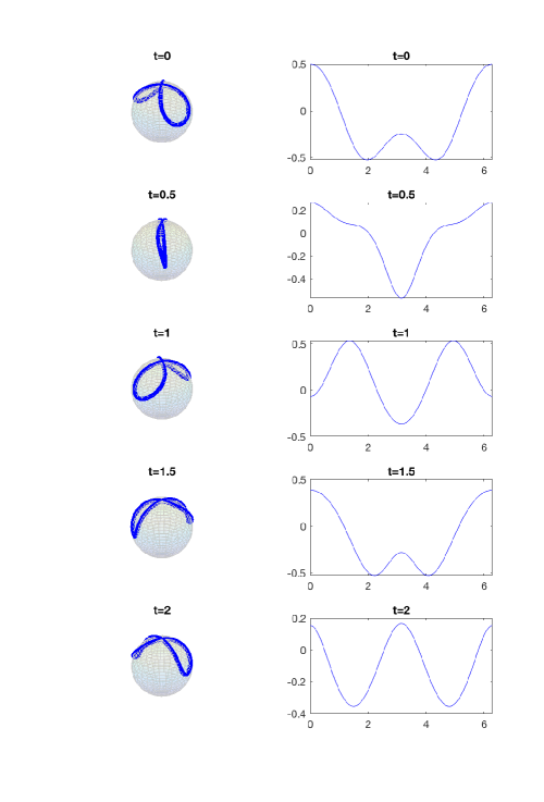
Figure 2: Numerical solution $\gamma_{num}$ versus the real part of the corresponding local invariant $q$ at $t=0,0.5,1,1.5,2$, respectively with $\triangle t=0.001$.

Spherical Sinusoid

Next example is to begin with

$$\gamma_{0}(x)=(\frac{\cos x}{\sqrt{1+\cos^{2}2x}},\frac{\sin x}{\sqrt{1+\cos^{2}2x}},\frac{\cos 2x}{\sqrt{1+\cos^{2}2x}}).$$

Fig. 3 shows the numerical results. The left column consists of Schrödinger curves obtained from the initial curve $\gamma_{0}(x)$ with $N=2^{10}$ and the time step $0.01$ at different time, paired with those curves from overhead viewpoint. At $t=3$ and $t=4$, the curves seem to have cusps only because of different perspectives. They are actually smooth. In Fig. 4, the drop-down parts of curve stretches. So we see that the drop-down parts slightly move to other places at each time in the right column of Fig. 4.

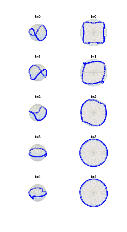
Figure 3: Numerical solution $\gamma_{num}$ (left) versus the projection of the $\gamma_{num}$ onto $xy$ plane (right) at $t=0,1,2,3,4$, respectively with $\triangle t=0.01$.

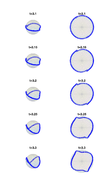
Figure 4: Numerical solution $\gamma_{num}$ (left) versus the projection of the $\gamma_{num}$ onto $xy$ plane (right) at $t=3.1,3.15,3.2,3,25,3.3$, respectively with $\triangle t=0.01$.

Schrödinger curve with $1$-soliton $q$

Based on our geometric scheme, we are able to obtain the first periodic solution $q$ of the NLS. Applying Bäcklund transformation to $q$ will give us one-soliton $\tilde{q}$. Proposition 2.5 and Theorem 2.8 imply that the new $\tilde{E}(x,t,\lambda)$ will give rise to a new solution of (1). As an example, we apply BT on the stationary solution, i.e., a great circle. Fig. 5 shows a numerical result with $\alpha=1-i,V={\mathbb{C}}\left(\begin{array}[]{c}1\\ i\end{array}\right)$.

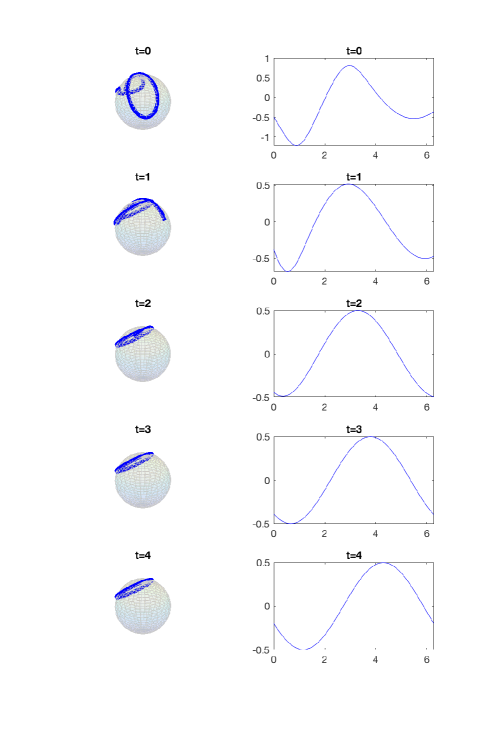
Figure 5: $\tilde{\gamma}_{num}$ constructed from applying BT on the circle versus the real part of the corresponding local invariant $q$ at $t=0,1,2,3,4$, respectively with $\triangle t=0.01$.

Figure 6: The real part of $1$-soliton solution $q_{1}$ corresponding $\tilde{\gamma}_{num}$ constructed from the circle with $q$ at $t=0,1,2,3,4,5$, respectively with $\triangle t=0.01$.

Remark 4.1.

The first picture in Fig. 5 indicates that the solution we get by applying the Bäcklund transformation might not be periodic. At $t=1$, two endpoints are approaching to each other. From the experimental outcomes, such curve remains the same circle as that on the last picture in Fig. 5 until $t=10$.

4.3 Vortex filament equation

Assume $\gamma(x,t)$ is a solution of the Schrödinger flow (1). Let

(58) $$\alpha(x,t)=\int_{0}^{x}\gamma(s,t)~{}ds+c(t),$$

where $c(t)$ is independent of $x$. It implies

$$\alpha_{t} =\int_{0}^{x}\gamma_{t}(s,t)~{}ds+c^{\prime}(t)$$

$$=\int_{0}^{x}\gamma\times\gamma_{xx}(s,t)~{}ds+c^{\prime}(t).$$

Note that the integrand is a total derivative, i.e.,

(59) $$\gamma\times\gamma_{xx}=(\gamma\times\gamma_{x})_{x},$$

so the above equation turns out to be

(60) $$\alpha_{t}=\gamma\times\gamma_{x}(x,t)-\gamma\times\gamma_{x}(0,t)+c^{\prime}(t).$$

It says from (60) that $\alpha(x,t)$ is a solution of (3) if and only if

(61) $$c^{\prime}(t)=\gamma\times\gamma_{x}(0,t).$$

Moreover, what we can say for periodicity is the following:

Proposition 4.2.

$\alpha(x,t)$ defined as (58) is periodic in $x$ with period $2\pi$ if a solution of the Schrödinger flow $\gamma(x,t)$ has the same $x$-period.

Proof 4.3.

Let

(62) $$y(t)=\alpha(2\pi,t)-\alpha(0,t).$$

Direct computation shows that

(63) $$y^{\prime}(t)=\gamma\times\gamma_{x}(2\pi,t)-\gamma\times\gamma_{x}(0,t).$$

Since $\gamma(x,t)$ is periodic in $x$ with period $2\pi$, so is $\gamma_{x}(x,t)$. It is clearly that $y^{\prime}(t)=0$, namely, $y(t)$ is a constant. As $y(0)=0$, we obtain $y(t)=0$ for all $t$. The assertion is proved.

An immediate example is when a great circle $\gamma(x,t)=(0,\cos x,\sin x)$ solves the Schrödinger flow, one can verify that $\alpha(x,t)=(t,\sin x,-\cos x)$ gives a solution of the vortex filament equation. Together with our geometric scheme mentioned in previous sections, a numerical solution of the vortex filament equation (3) has been provided.

On the other hand, an algebraic construction of periodic solution for the vortex filament equation

(64) $$\begin{cases}\alpha_{t}=\alpha_{x}\times\alpha_{xx}\\ \alpha(x,0)=\alpha_{0}\end{cases},$$

has been given by Terng where $\alpha_{0}:[0,2\pi]\to{\mathbb{R}}^{3}$ is a smooth arc-length parametrized curve periodic in $x$ with period $2\pi$. Equivalently, a geometric scheme follows from such construction in [10]. We summarize her ideas without proof.

Theorem 4.4.

Let $\alpha(x,t)$ be a solution of the VFE (3) that is periodic in $x$ with period $2\pi$ and $\,\|\,\alpha_{x}\,\|\,=1$. Suppose $(e_{0},\vec{n}_{1},\vec{n}_{2})$ is orthonormal along $\alpha$ such that $e_{0}=\alpha_{x}.$ Let $\omega=(\vec{n}_{1})_{x}\cdot\vec{n}_{2}$. Then

(65) $$c_{0}=\frac{1}{2\pi}\int_{0}^{2\pi}\omega(x,t)~{}dx$$

is constant for all $t$, and there is $g=(u_{0},u_{1},u_{2})(x,t)$ such that

1. $g(\cdot,t)$ is a periodic h-frame along $\alpha(\cdot,t)$,

2. $g^{-1}g_{x}=\left(\begin{array}[]{ccc}0&-\zeta_{1}&-\zeta_{2}\\ \zeta_{1}&0&-2c_{0}\\ \zeta_{2}&2c_{0}&0\end{array}\right)$,

3. $q=\frac{1}{2}(\zeta_{1}+i\zeta_{2})$ solves the nonlinear Schrödinger equation

   (66) $$q_{t}=\frac{i}{2}(q_{xx}+2|q|^{2}q).$$

Proposition 4.5.

Let $q$ be a solution of (66) periodic in $x$ with period $2\pi$, $\lambda_{0}\in{\mathbb{R}}$, and $E(x,t,\lambda)$ the extended frame of $q$. If $E(x,0,\lambda_{0})$ is periodic in $x$ with period $2\pi$, then so is $E(x,t,\lambda_{0})$.

Proposition 4.6.

Suppose $\alpha_{0}(x):{\mathbb{R}}^{2}\to{\mathbb{R}}^{3}$ is a periodic curve parametrized by arc-length with period $2\pi$. Let $(u_{0}^{0},u_{1}^{0},u_{2}^{0})$ be a $h$-frame $2q_{1}^{0},2q_{2}^{0}$ and $\phi\in SU(2)$ such that

(67) $$(u^{0}_{0},u^{0}_{1},u^{0}_{2})=(\phi a\phi^{-1},\phi b\phi^{-1},\phi c\phi^{-1}).$$

Suppose $q:{\mathbb{R}}^{2}\to{\mathbb{C}}$ is a periodic solution of

(68) $$\begin{cases}q_{t}=\frac{i}{2}(q_{xx}+2|q|^{2}q),\\ q(x,0)=q_{1}^{0}+iq_{2}^{0}.\end{cases}$$

Let $E$ be the extended frame with initial data $E(0,0,c_{0})=\phi,\eta=E_{\lambda}E^{-1}\ |\ _{\lambda=c_{0}},$ and $\alpha(x,t)=\eta(x-2c_{0}t,t)$. Then $\tilde{\alpha}(x,t)=\alpha(x,t)-\eta(0,0)+\alpha_{0}(0)$ solves (64) and is periodic in $x$ with period $2\pi$.

The geometric algorithm to solve (64) follows from the above discussion, we demonstrate experimental results here.

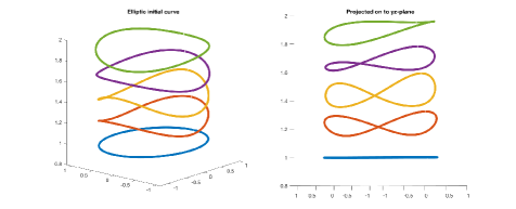
Figure 7: Curve motion starting with the bottom curve $\alpha_{0}(x)=(\cos x,\sin x,\cos x)$.

Starting with the bottom curve $\alpha_{0}(x)=(\cos x,\sin x,\cos x)$ (left), this curve slowly floats up as time goes by. Such simulation shows that it captures the smoke ring feature for the vortex filament equation.

5 Discussion of error estimates

At a fixed time, Table 1 shows that the $L^{2}$-error $E_{N}(t)$ decreases when the number of grid points $N$ is increase. Indeed, from the experimental results, we see that $\frac{E_{2N}(t)}{E_{N}(t)}$ is approximately located in between $\frac{1}{4}$ and $\frac{1}{2}$.

We also notice that if $N$ is fixed, the error $E_{N}(t)$ accumulates at each time step in Table 1. For the total time $T=1$, we see the errors $G_{N}^{sup}$ in Table 3. As for the data demonstrated, the error becomes half of itself when we reduce time step by a half, provided $N$ is fixed. The error estimates shown are not so impressed in a sense of numerics. One reason why this error is not ”so small” is that we use the WGMS method to approximate the solution $q$ to the NLS. Several types of numerical errors come from the WGMS algorithm, including the obvious error in approximating the integral and a truncation error when the fixed point iteration was stopped after a finite number of steps.

Another reason is that we simply use finite difference method to obtain numerical results for the frame $E$ in (44) with the right hand side filled out with the estimated $q$. This of course increases errors. It also indicates the numerical scheme can be improved by choosing other more accurate ODE solvers.

6 Conclusions

Although the accuracy provided is not relatively impressed, this geometric algorithm shows that using simple solvers for each piece in the implement can help to get numerical solutions ”good enough” to the nonlinear curve PDE (1). The advantage of this method is transform the nonlinearity of curve motion to solving the ODE system (44). Each step can be solved numerically by built-in functions in MatLab, therefore our scheme is easier for beginners to do programming. The price to pay from the experimental results is obviously some accuracy. However, it is expected that experts in coding can have better approximations if they work more on each step of the implement.

References

• [1] J. Bourgain, Fourier transform restriction phenomena for certain lattice subsets and applications to nonlinear evolution equations. i. schrdinger equations, Geom. Funct. Anal., 3 (1993), pp. 107–156.
• [2] J. Bourgain, Periodic nonlinear schrödinger equation and invariant measures, in Commun. Math. Phys. 166, 1-26, 1994.
• [3] H. Hasimoto, Motion of a vortex filament and its relation to elastic, in J. Phys. Soc. Jap. 31, 293-295, 1971.
• [4] T. Y. Hou, I. Klapper, and H. Si, Removing the stiffness of curvature in computing 3-d filaments, in J. Comput. Phys. 143, 628-664, 1998.
• [5] T. Y. Hou, J. S. Lowengrub, and M. J. Shelley, Removing the stiffness from interfacial flows with surfce tension, in J. Comput. Phys. 114, 312-338, 1994.
• [6] A. R. Its, Inversion of hyperelliptic integrals, and integration of nonlinear differential equations, (Russian. English summary) Vestnik Leningrad. Univ. 1976, no. 7 Mat. Meh. Astronom., 2 (1976), pp. 39–46.
• [7] T. C.-L. Liu, H.-F. and Z. Wu, Darboux-bäcklund transformations for nls-systems, (2018).
• [8] R. S. Palais, The initial value problem for weakly nonlinear pde, in Journal of Fixed Point Theory and Applications 16(1-2), 2015.
• [9] L. A. Takhtajan, Integration of the continuous heisenberg spin chain through the inverse scattering method, Physics Letters, 64A (1977), pp. 235–237.
• [10] C. Terng, Dispersive geometric curve flows, in Surv. Differ. Geom., 19, Int. Press, Somerville, MA, 2015.
• [11] C. Terng and G. Thorbergsson, Completely integrable curve flows on adjoint orbits, in Dedicated to Shiing-Shen Chern on his 90th birthday, Results Math. 40, pp. 286–309, 2001.
• [12] C. Terng and K. Uhlenbeck, Bäcklund transformations and loop group actions, in Comm. Pure. Appl. Math. 53, 1-75, 2000.
• [13] C. Terng and K. Uhlenbeck, Schrödinger flows on grassmannians, in Integrable systems, Geometry, and Topology, AMS/IP Stud. Adv. Math. 36, 235-256, 2006.
• [14] J. Tjon and J. Wright, Solitons in the continuous heisenberg spin chain, Physical Review B, 15 (1977), pp. 17–23, https://doi.org/10.1103/PhysRevB.15.3470.
• [15] V. Zakharov and L. Takhtadzhyan, Equivalence of the nonlinear schrödinger equation and the equation of a heisenberg ferromagnet, Theoretical and Mathematical Physics(Russian Federation), 38 (1979), pp. 17–23, https://doi.org/10.1007/BF01030253.