Kepler Planet Occurrence Rates for Mid-Type M Dwarfs as a Function of Spectral Type

Abstract

Previous studies of planet occurrence rates largely relied on photometric stellar characterizations. In this paper, we present planet occurrence rates for mid-type M dwarfs using spectroscopy, parallaxes, and photometry to determine stellar characteristics. Our spectroscopic observations have allowed us to constrain spectral type, temperatures, and in some cases metallicities for 337 out of 561 probable mid-type M dwarfs in the primary Kepler field. We use a random forest classifier to assign a spectral type to the remaining 224 stars. Combining our data with Gaia parallaxes, we compute precise ($\sim$3%) stellar radii and masses, which we use to update planet parameters and planet occurrence rates for Kepler mid-type M dwarfs. Within the Kepler field, there are seven M3 V to M5 V stars which host 13 confirmed planets between 0.5 and 2.5 Earth radii and at orbital periods between 0.5 and 10 days. For this population, we compute a planet occurrence rate of $1.19^{+0.70}_{-0.49}$ planets per star. For M3 V, M4 V, and M5 V, we compute planet occurrence rates of $0.86^{+1.32}_{-0.68}$, $1.36^{+2.30}_{-1.02}$, and $3.07^{+5.49}_{-2.49}$ planets per star, respectively.

1 Introduction

The NASA Kepler mission (Borucki et al., 2010) revolutionized astrophysics and planetary science. Kepler has enabled the discovery of 2,342 new exoplanets and an additional 2,421 planet candidates. Four years of data from the original Kepler mission have provided light curves for nearly 200,000 stars (Mathur et al., 2017) from which we can estimate the statistical distribution of planet properties within our Galaxy.

Kepler was designed to detect Earth-sized planets in the habitable zones of Sun-like (F, G, and K) stars. M dwarfs ($2,300\,\mathrm{K}\lesssim T_{\mathrm{eff}}\lesssim 3,900\,\mathrm{K}$, $0.1\,R_{\odot}\lesssim R_{\star}\lesssim 0.6\,R_{\odot}$, $0.07\,M_{\odot}\lesssim M_{\star}\lesssim 0.6\,M_{\odot}$) comprise about $70\%$ of the nearby stellar population, by number (Henry et al., 2006; Bochanski et al., 2010), though they only constitute about 2.5% of the targets Kepler observed (Dressing & Charbonneau, 2015, hereafter DC15). The smaller size of these stars makes it easier to detect the presence of smaller transiting planets. For example, the transit depth for an Earth-radius planet transiting a solar metallicity M0 V star would be 3 times deeper than the same planet transiting a G2 V Sun-like star, and nearly 70 times deeper for an M7 V star. Fortuitously, the low luminosity of M dwarfs means the habitable zone is closer to the star, thus increasing the chance of detecting a transiting planet in the habitable zone over a finite observing period (Nutzman & Charbonneau, 2008). For example, an Earth-sized planet in the habitable zone of an M4 V star orbits once every two weeks as opposed to once a year for a Sun-like G star.

Planet occurrence rates increase toward later spectral types within the Kepler field. Using the first three quarters of Kepler data, Howard et al. (2012) measured the planet occurrence rate for M0 to F2 dwarfs for planets with radii between 2 and $4\,R_{\oplus}$ and found that these small planets are seven times more abundant around cool stars (3,600 to $4,100\,\mathrm{K}$) than hot stars (6,600 to $7,100\,\mathrm{K}$). More recent work by Mulders et al. (2015a) found the occurrence rate of planets with radii between 1 and $4\,R_{\oplus}$ around M dwarfs to be two times higher than for G stars, and three times higher than for F stars. Dressing & Charbonneau (2013, hereafter DC13) focused specifically on stars with temperatures below $4,000\,\mathrm{K}$ in Q1 to Q6 of Kepler data and found the occurrence rate of 0.5 to $4\,R_{\oplus}$ planets with orbital periods shorter than 50 days to be $0.90^{+0.04}_{-0.03}$ planets per star. Separating these stars into warmer ($T_{\mathrm{eff}}>3,400\,\mathrm{K}$) and cooler ($T_{\mathrm{eff}}<3,400\,\mathrm{K}$) groups, they find the occurrence rate of Earth-sized planets (0.5 to $1.4\,R_{\oplus}$) to be consistent at around 0.5 planets per star, but the rate of larger planets (1.4 to $4.0\,R_{\oplus}$) is three times higher for the warmer stars, $0.61^{+0.08}_{-0.06}$ compared to $0.19^{+0.07}_{-0.05}$. Using the full Kepler data set, DC15 updated their M dwarf planet occurrence rate for 1 to $4\,R_{\oplus}$ planets with orbital periods shorter than 200 days to be $2.5\pm 0.2$ planets per star, but they do not make a distinction between early and mid-type M dwarfs. Gaidos et al. (2016b) computed an overall Kepler M dwarf planet occurrence rate of $2.2\pm 0.3$ for orbital periods shorter than 180 days, consistent with DC15. Focusing specifically on mid-type M dwarfs, Muirhead et al. (2015) calculated a compact multiple occurrence rate of $21^{+7}_{-5}\%$, assuming a radius of $0.2\,R_{\odot}$ for all mid-type M dwarfs.

Computing planet occurrence rates requires measurements of stellar radii ($R_{\star}$) for all stars in the sample population. In the absence of direct measurements, $R_{\star}$ for the M dwarfs in the Kepler Input Catalog (KIC) was derived from optical and infrared photometry (Batalha et al., 2010; Brown et al., 2011). Brown et al. (2011) noted that stellar parameters in the KIC are unreliable at $T_{\mathrm{eff}}<3,750\,\mathrm{K}$ because the models they use are calibrated to work best for Sun-like stars. DC13, Gaidos (2013), and Huber et al. (2014) addressed this issue by using stellar models more suited to later type stars (e.g., Dartmouth Stellar Evolution Database; Dotter et al., 2008) to reclassify the set of cooler stars in the KIC. These updated measurements of $R_{\star}$, based on photometry, still have a wide range of uncertainties with an average around 30% (Mathur et al., 2017). An uncertainty this large can mean the difference between several spectral sub-types, and for a transiting planet this propagates to a 30 to 40% planet radius uncertainty.

Combining long-baseline optical interferometry with trigonometric parallax measurements yields direct measurements of stellar radii with uncertainties between 1% and 5%; however, this method is currently limited to bright ($V\lesssim 11$), nearby stars (e.g., Ségransan et al., 2003; Boyajian et al., 2012; von Braun et al., 2014). These precise radius measurements can, however, be used to calibrate empirical relationships between radius and other measurable parameters (e.g., Boyajian et al., 2012; Mann et al., 2015). For example, Mann et al. (2015, hereafter M15) derive $M_{K_{s}}$ vs. $R_{\star}$ and $T_{\mathrm{eff}}$ vs. $R_{\star}$ relationships for K7 through M7 dwarfs, which constrain stellar radii to $\sim$3% and $\sim$15%, respectively. Gaidos et al. (2016b) used these relationships to update the stellar properties of over 4,000 Kepler M dwarfs based on temperatures, metallicities, and distances derived from photometry and proper motions. These measurements constrain stellar radii to $\sim$15%.

With moderate resolution spectra, we can precisely determine spectral type and measure stellar properties such as temperature and metallicity. Having accurate spectral types for a specific population (e.g., mid-type M dwarfs) allows us to assess trends in planet occurrence rates for that population as a function of spectral type, like the assessment of F, G, K, and early M dwarf planet occurrence rates by Howard et al. (2012). In large stellar catalogs, such as the KIC, it is difficult to obtain a spectrum of each star, so photometric selection criteria are typically used to identify specific stellar populations (e.g., Brown et al., 2011; Dressing & Charbonneau, 2013; Gaidos, 2013; Huber et al., 2014; Gaidos et al., 2016b). Efforts to spectroscopically classify nearly 5,000 photometrically-identified late-type K and M dwarfs in the Kepler field by Mann et al. (2012), Muirhead et al. (2012), Mann et al. (2013b), and Martín et al. (2013) have yielded spectra for only $2\%$ of the sample (DC15). While selection criteria aim to minimize stellar outliers, they are not impervious to contamination. Spectra allow us to identify any interlopers (such as giant stars) that selection criteria might not cull.

In this paper we present spectroscopic observations of 333 M dwarfs and 4 M giants in the Kepler field, from which we derive spectral types, effective temperatures, and metallicities. Thanks to the European Space Agency’s Gaia mission (Gaia Collaboration et al., 2016), nearly all the stars in the Kepler field now have trigonometric parallax measurements (Berger et al., 2018). Over $90\%$ of our targets have Gaia parallax measurements, which we use to compute $M_{K_{s}}$. We apply the empirical relationships of M15 and Mann et al. (2019) to measure radii and masses for our stars. With these updated stellar properties, we refine the properties for the 13 confirmed planets around mid-type M dwarfs. We then compute the total planet occurrence rate for mid-type M dwarfs, individual occurrence rates for M3 V, M4 V, and M5 V stars, and compact multiple occurrence rates.

Figure 1: Magnitude distributions in (a) $r$-band and (b) $K_{s}$-band of Kepler targets for this survey. The orange solid line histograms represent all targets, the blue dashed line histograms are the targets for which we have an optical spectrum, and the red dashed dotted line histograms show targets for which we have an infrared spectrum. The optical spectra distribution closely follows the distribution of all targets in the sample. Targets were selected to optimize observation efficiency with WIYN by maximizing the number of targets observed per field configuration. Several fainter targets were also observed with the Discovery Channel Telescope. This strategy allowed us to effectively observe a random sample representing the total target set. Almost all stars with infrared spectra have $K_{s}<13$, since fainter targets necessitate much longer integration times to obtain sufficient S/N to measure stellar properties.

In Section 2 we describe our target selection, spectroscopic observations, and Gaia data. We explain our methods for determining stellar properties in Section 3, and refine our sample to reject giant stars and close binaries in Section 4. In Section 5 we identify the planets around mid-type M dwarfs in the Kepler field, which we use for our planet occurrence rate calculations in Section 6. We conclude with a discussion in Section 7.

2 Target Selection, Observations, and Data Reduction

Using revised KIC temperature estimates, DC13 identified 202 stars with $T_{\rm{eff}}\lesssim 3,300\,\mathrm{K}$. Muirhead et al. (2015) identified 509 probable mid-type M dwarfs from KIC photometry using the following color selection criteria: $r-J>3.2$ to identify red objects, and $J-K<0.0555\times(r-J)+0.7622$ to remove giant stars. The union between these samples produces 561 probable mid-type M dwarfs which we targeted in this study. In total, we observed 337 of the 561 targets (60%), obtaining optical spectra of 327 stars and near-infrared spectra of 82 stars. We have both optical and infrared spectra for 72 targets. Magnitude distributions of our targets in $r$-band and $K_{s}$-band are shown in Figure 1, including the distributions of targets we observed.

2.1 WIYN

In observing semester 2015B, NASA and NSF implemented Stage 1 of the Exoplanet Observational Research (NN-EXPLORE) program, enabling community access to about 100 nights per year on the 3.5-meter WIYN telescope on Kitt Peak at least through commissioning of the extreme precision Doppler spectrometer NEID (Schwab et al., 2016). We have made use of the fiber-fed multi-object spectrograph Hydra (Barden et al., 1994) on WIYN for this project. The Kepler field spans a 12 degree diameter, making the one degree diameter field-of-view of Hydra advantageous. We collected spectra over five observing semesters beginning in September 2015 (NOAO Program IDs 2015B-0280, 2016A-0328, 2016B-0111, 2017A-0185, 2017B-0095; PI: K. Hardegree-Ullman). In total, we observed 287 targets with WIYN.

Each Hydra field configuration contained an average of five mid-type M dwarf targets with $V<18.5$. We used the bench spectrograph camera and the red optimized fiber cable containing 90 fibers. The 316 lines mm^-1 grating and the G5 filter were used to obtain spectra spanning 5,000 to 10,000 Å with an average resolving power $R=\lambda/\Delta\lambda\approx 1,420$. Most fields were observed in three consecutive 1,200 second exposures to mitigate the effect of cosmic rays and to yield a signal-to-noise (S/N) of at least 30 per resolution element for targets with $V<18.5$. At the beginning and end of each night we obtained bias, dome flat field, and copper-argon wavelength calibration frames. After each field observation, we obtained a spectrum of a nearby bright G0 star at a similar airmass to be used for telluric correction. At least once each night we observed a spectrophotometric standard star for relative flux calibration.

The data were reduced using IRAF and custom IDL routines. Each image was first corrected for readout bias using the overscan strip, then trimmed to remove this region. An average bias was then created and subtracted from the rest of the images. The dohydra IRAF routine was used for aperture extraction, flat fielding, dispersion correction, and sky subtraction. Sky spectra were created from 5 to 10 sky fibers placed in random positions distributed throughout each field. Sky subtraction removed OH atmospheric emission, which is problematic at wavelengths redder than 6,000 Å. Individual exposures were then combined, and a relative flux calibration was performed on all targets using a spectrophotometric standard star. We developed a custom IDL script to interpolate across a G0 star spectrum where there is known atmospheric absorption, and divide these regions out of our M dwarf spectra to remove terrestrial atmospheric absorption features. We shift each spectrum in wavelength to the source star’s rest frame by cross-correlation with the closest matching M dwarf template from Bochanski et al. (2007). We find the closest matching M dwarf template from a by-eye comparison of each spectrum to each template, normalized to 8,350 Å.

2.2 Discovery Channel Telescope

About 90 of our targets have $V$-band magnitudes fainter than 18.5, which would require integration times longer than one hour using WIYN to achieve a S/N of 30. We therefore used the DeVeny spectrograph on the 4.3-meter Discovery Channel Telescope (DCT) to observe some of these fainter targets over four observing runs, collecting spectra of 49 stars. We observed 17 of these stars with WIYN because they were within one of the observed WIYN fields. These targets are used to check for consistency between the two telescopes, though the DCT data are higher resolution.

The DeVeny spectrograph is a single-slit instrument with a deep depletion e2v CCD. The 400 grooves mm^-1 grating and OG570 filter were used to obtain spectra spanning 6,300 to 9,700 Å with $R\approx 2,850$. Total integration times varied in order to achieve a S/N similar to WIYN targets, and at least three consecutive exposures were taken of each target to mitigate cosmic rays in the data reduction. Calibrations were the same as for WIYN, except for the neon-argon lamps used for wavelength calibration. Data reduction was again performed in IRAF using the same steps as for WIYN data, but with single slit routines instead of dohydra.

2.3 IRTF

We used the SpeX spectrograph (Rayner et al., 2003) on the NASA Infrared Telescope Facility (IRTF) on Maunakea to observe 82 targets over 12 partial nights (Program IDs 2016A-981, 2017A-106, 2017B-021; PI: K. Hardegree-Ullman). We used SpeX in SXD mode with a $0\farcs 3\times 15\arcsec$ slit to obtain 0.8 to $2.4\,\mu$m spectra at $R\approx 2,000$. We observed using the ABBA nod pattern with at least three exposures for each target. Exposure times were shorter than 120 seconds to minimize effects from atmospheric OH line variability. For most targets we achieved a S/N of at least 50 per resolution element. An A0 V star was observed within 0.1 airmasses of each target to be used for telluric correction and flux calibration. Flat field and thorium-argon lamp calibrations were taken after each A0 V star observation.

Spectra were reduced using Spextool (v. 4.2; Cushing et al., 2004), which performs flat fielding, wavelength calibration, sky subtraction, and spectrum extraction. We used the xtellcor IDL package (Vacca et al., 2003) for telluric correction. As with each optical spectrum, we shift each infrared spectrum in wavelength to the source star’s rest frame by cross-correlating with a spectrum of corresponding spectral type from the IRTF spectral library (Cushing et al., 2005; Rayner et al., 2009).

2.4 LAMOST

The Large Sky Area Multi-Object Fiber Spectroscopic Telescope (LAMOST; Cui et al., 2012) is a 4-meter class telescope designed to survey stars and galaxies in the northern hemisphere. Its 4,000 fiber multi-object spectrograph has a wavelength range of 3,690 to 9,100 Å at $R\approx 1,800$. As of data release 4, over 7.6 million spectra have been gathered in total. There are LAMOST spectra for 17 of our Kepler targets, including 8 targets we did not observe with WIYN or the DCT. This brings our total optical spectra count to 327 targets.

2.5 Gaia

The Gaia mission has provided parallax measurements for over 1.3 billion sources in second data release (Gaia Collaboration et al., 2018). Bailer-Jones (2015) and Bailer-Jones et al. (2018) note that simply inverting the parallax does not always produce reliable distances. Instead, distances must be inferred via probabilistic analysis, which Bailer-Jones et al. (2018) performed on all targets in the second Gaia data release, providing distance measurements and uncertainties. We use the Gaia/Kepler cross-match database to obtain the Bailer-Jones et al. (2018) Gaia distances to our Kepler stars. In total, 532 of our targets cross-match with a Gaia target within 4″, the Kepler pixel size. We also check the difference between the Gaia $G$-band ($\gtrsim 20\%$ transmission between 4,000 and 9,000 Å; Evans et al., 2018) and Kepler $Kp$-band ($\gtrsim 20\%$ transmission between 4,300 and 8,900 Å) magnitudes. For any target with an absolute $G-Kp$ magnitude difference greater than 2, we discard the parallax measurement in our analysis, which applies to KIC 02164791, KIC 03330684, KIC 07729309, and KIC 10665619.

3 Stellar Properties

We seek to determine planet occurrence rates for mid-type M dwarfs using revised stellar radius measurements derived from spectra, photometry, and parallaxes. About 95% of our targets have parallax measurements, which allows us to compute absolute magnitudes in the $r$, $J$, and $K_{s}$-bands for use in computing stellar properties (Section 3.1). For the 337 targets with spectra, we do a by-eye comparison to spectral templates to determine spectral types. There are 224 targets for which we do not have spectra, so we use a machine learning technique to identify spectral type from photometry (Section 3.2). Using a spectral type vs. temperature relationship, we derive stellar temperatures (Section 3.3). For targets with infrared spectra, we determine metallicity (Section 3.4). We apply the $M_{K_{s}}$ vs. radius and $M_{K_{s}}$ vs. mass relationships of M15 and Mann et al. (2019) to derive stellar radii and masses for targets with parallax measurements. For the remaining targets, we derive radii from a temperature vs. radius relationship (Section 3.5) and masses from a radius vs. mass relationship (Section 3.6). With our updated spectral types, we isolate mid-type M dwarfs, and compute planet occurrence rates for spectral types M3 V to M5 V using our new stellar properties (Section 6). We present all derived stellar parameters in Tables 3 and 4.

3.1 Absolute Magnitudes

For targets with Gaia parallax measurements, we compute absolute magnitudes $M$ for Sloan Digital Sky Survey (SDSS; York et al., 2000) $r$-band and Two Micron All-Sky Survey (2MASS; Skrutskie et al., 2006) $J$ and $K_{S}$-bands using

$$M=m-5[\log_{10}(d)-1]-A,$$ (1)

where $m$ is the apparent magnitude for a photometric band, $d$ is the distance in parsecs, and $A$ is the extinction for that photometric band. We compute reddening vectors using the 3D dust maps of Green et al. (2018) with the Python package dustmaps. We find extinction for each band by multiplying the reddening vectors by the extinction coefficients $R$ from Green et al. (2018), which are 2.483, 0.650, and 0.161 for $r$, $J$, and $K_{s}$ bands, respectively. We calculate absolute magnitudes and their associated uncertainties for each band using the following Monte Carlo (MC) analysis. For each measured parameter we generate $10^{4}$ random samples from a Gaussian distribution and combine these distributions for each calculation. The uncertainties for each quantity are symmetric or nearly symmetric within a few percent, so we use the mean of any asymmetric uncertainty to draw our Gaussian distribution. The absolute magnitude is then the median value of the posterior distribution, and we adopt the 16^th and 84^th percentiles as the uncertainties.

3.2 Spectral Type

We determine optical spectral types by comparing our spectra to the SDSS M dwarf spectral templates of Bochanski et al. (2007), following the methods of Kirkpatrick et al. (1991). The template spectra span a wavelength range of 3,800 to 9,200 Å with $R\approx 1,800$. Target spectra are normalized to the same wavelength as the template spectra (8,350 Å) and we do a by-eye comparison to find the closest matching spectrum to the nearest half spectral type. Ten of our targets were only observed with IRTF. For these targets, we determine spectral type in the same manner as our optical spectra, except we use M dwarfs in the IRTF Spectral Library for comparison (Cushing et al., 2005; Rayner et al., 2009).

It is always best to determine spectral type from a spectrum rather than photometry, however, this is not always economical with a large target sample and limited resources. For the 224 stars in our sample that lack a spectrum, we use the RandomForestClassifier routine from the scikit-learn (Pedregosa et al., 2011) Python package to classify these targets with $r$, $J$, and $K_{s}$-band photometry. For our training sample, we use the extinction corrected photometry and spectral types from West et al. (2011), who visually inspected over 70,000 M dwarf spectra from SDSS. We truncate this data set to include spectral types M0 to M8, and use the color cut $J-K_{s}<0.0555\times(r-J)+0.7622$ to reflect the targets in our sample. From these 48,978 targets, we randomly select 1,500 from each spectral type to minimize sample bias, reducing our input sample to 13,500 targets. Using the $r-J$ and $J-K_{s}$ colors along with spectral type, we train the random forest classifier on a random subset of 75% of the total input sample. The remaining 25% of the input sample is used to determine how well the classifier performs. Figure 2 compares the observed spectral type from spectra to the predicted spectral type from the classifier. Over 90% of the predicted classifications are within one spectral type of the observed spectral type, so we adopt an uncertainty of $\pm 1$ spectral type for our photometric classifications.

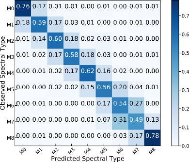
Figure 2: Comparison of the fraction of predicted classifications in each spectral type bin versus observed spectral type from a random forest classification using photometry from the West et al. (2011) M dwarf sample. Over 90% of the predicted classifications are within one spectral type of the observed spectral type.

We run the trained classifier on the photometry for both our spectroscopically observed and unobserved targets. In the case of the 530 targets for which we have Gaia parallax measurements, we use extinction corrected absolute magnitudes to compute $r-J$ and $J-K_{s}$ colors. The average difference between the colors computed from absolute magnitudes versus apparent magnitudes is about 0.03 for each color, which is the small effect of the reddening correction. For the remaining 31 targets without parallax measurements, we use apparent magnitudes to compute colors. The classifier predicts 86% of the spectral types of our spectroscopically observed sample to within one spectral type, however, it over-predicts M3 V by a factor of 2, and significantly under-predicts M2 V and M7 V, as shown in Figure 3 a. For the photometric sample, the distribution of spectral types roughly follows the same distribution as the spectroscopic sample. We also show the spectral type distribution for the entire sample in Figure 3 b. Since we effectively observed a random subset of mid-type M dwarfs in the Kepler field, we expect the photometrically classified targets to follow a similar spectral type distribution to the spectroscopically classified targets, and thus we are confident in the results from the photometric classification.

Figure 3: (a) Comparison of observed (solid orange) versus predicted (dashed blue) spectral type distributions using the random forest classifier on the Kepler targets we have spectroscopically classified. (b) The spectral type distribution for our entire Kepler sample using results from spectra for observed targets (solid green), and the classifier (dashed magenta) on stars without spectra. The photometric histogram is stacked on top of the spectroscopic histogram. For these histograms, stars with half spectral types are rounded up to the nearest integer type.

3.3 Effective Temperature

Direct measurement of effective temperatures requires both bolometric flux and interferometric angular diameter measurements. Due to the distance and faintness of these stars, interferometric observations are not currently possible. Using the spectral types and effective temperatures of the 183 stars in Table 5 of M15, we determine a linear spectral type vs. effective temperature relationship:

$$T_{\mathrm{eff}}=-168.37\times SpT+3914.65,$$ (2)

where $SpT$ is the spectral type between $-1$ for K7 V and 7 for M7 V. We adopt this as a uniform temperature scale across our spectroscopic and photometric sample. The residual 1-$\sigma$ scatter of our fit to the M15 spectral types and temperatures is $64\,\mathrm{K}$, which we add in quadrature to the typical $60\,\mathrm{K}$ spectroscopic measurement uncertainties. This yields $88\,\mathrm{K}$, which we adopt as our temperature uncertainty.

Pecaut & Mamajek (2013) determine effective temperatures for each sub-type of main sequence stars by taking the median values of published effective temperatures in the literature. As a consistency check to our M15 fit, we take the most recent list of all reported values used to compute the median effective temperature for each sub-type between K7 V and M9 V (280 stars) and fit a linear relationship. This results in $T_{\mathrm{eff}}=-166.96\times SpT+3868.39$, with a $107\,\mathrm{K}$ 1-$\sigma$ scatter. This relationship gives temperatures on average $40\,\mathrm{K}$ cooler than our temperatures. We also compare our temperatures to the M dwarf temperature scale of Rajpurohit et al. (2013), which are on average $76\,\mathrm{K}$ cooler than our temperatures. All three methods yield temperatures which are consistent within the measurement uncertainties.

3.4 Metallicity

We computed metallicities (specifically, iron abundance, [Fe/H]) for 82 targets we observed with SpeX on IRTF. Mann et al. (2013a, 2014) determined metallicity of M dwarfs in wide binary systems with an F, G, or K primary star, and computed empirical relationships between metallicity and equivalent widths of Na I and Ca I using infrared spectra from SpeX. Our metallicity measurements using these relationships are listed in Table 3. We did not obtain infrared spectra of any of the mid-type M dwarf planet hosts (Table 2), however, we adopt the metallicity measurements of Kepler-42, Kepler-445, and Kepler-1650 from Mann et al. (2017), Kepler-446 and Kepler-1582 from Muirhead et al. (2014), and Kepler-1649 from Angelo et al. (2017). All of these metallicity measurements were made using the same relationships from Mann et al. (2013a). The only planet host for which we do not have a metallicity measurement is Kepler-1646.

Figure 4: (a) Comparison of our radius measurements of Kepler M dwarfs to radii from the Kepler Stellar Catalog (Mathur et al., 2017). We do not include 17 targets from the Kepler Stellar Catalog with $R_{\star}>1\ R_{\odot}$. The 1:1 reference line is plotted in red, and median uncertainties are shown in the upper left corner. The histograms show the radius measurement distributions. (b) Comparison of our radius measurements to those from DC13 for the 213 targets found in both samples. (c) Comparison of our radius measurements to those from Gaidos et al. (2016b) for the 399 targets found in both samples. Our radii are generally larger than previous measurements.

3.5 Radius

For the 95% of targets with distance measurements, we apply the $M_{K_{s}}$ vs. $R_{\star}$ and $M_{K_{s}}$ vs. [Fe/H] vs. $R_{\star}$ relationships of M15 to compute stellar radii, which have model fit uncertainties of 2.89% and 2.70%, respectively. We employ the same MC analysis from Section 3.1 to assess parameter uncertainties, and add them to the model uncertainties in quadrature, which yields a median 3.13% and 2.85% radius uncertainty, respectively.

Not all of our targets have distance measurements, so we rely on the M15 $T_{\mathrm{eff}}$ vs. $R_{\star}$ and $T_{\mathrm{eff}}$ vs. [Fe/H] vs. $R_{\star}$ relationships to get the remaining stellar radii. Adding in quadrature the 13.4% ($T_{\mathrm{eff}}$ vs. $R_{\star}$) and 9.3% ($T_{\mathrm{eff}}$ vs. [Fe/H] vs. $R_{\star}$) uncertainties to values from the MC analysis, we yield median uncertainties of 20.6% and 18.6%, respectively, for these targets.

In Figure 4 we compare our new stellar radius measurements to those reported in the Kepler Stellar Catalog (Mathur et al., 2017), 213 of our targets also found in DC13, and 399 stars in Gaidos et al. (2016b). Both the Kepler Stellar Catalog and DC13 show a similar radius distribution for most targets, with a peak near $0.2\,R_{\odot}$, whereas our measurements are generally larger by $\sim$58%. Our radii are more consistent with those reported in Gaidos et al. (2016b), but our use of distances from Gaia yield more precise values of $M_{K_{s}}$, resulting in $\sim$20% larger radii.

3.6 Mass

We apply the $M_{K_{s}}$ vs. $M_{\star}$ relationship of Mann et al. (2019) to compute stellar masses of targets with distance measurements using the Python code provided with that paper. This yields median uncertainties of 2.59% and 2.64% for targets with and without metallicity measurements, respectively. For the 28 targets without $M_{K_{s}}$ measurements we need another method to compute mass. We fit the mass and radius measurements for 183 M dwarfs in M15 with a third degree polynomial using the polyfit routine in the numpy (Oliphant, 2015) Python package and find:

$$M_{\star}=-0.01+0.63R_{\star}+1.34R_{\star}^{2}-0.99R_{\star}^{3}.$$ (3)

The root-mean square scatter of this fit is 3.75%. We apply Equation 3 to the targets for which we do not have distance measurements in the same manner as our previous model fits and yield a median 33.2% mass uncertainty for these targets.

4 Refining the Sample

Our target selection criteria were chosen to isolate M dwarfs, but that does not preclude a few giant or binary interlopers. From our spectra, we identify four giants (Section 4.1), two eclipsing binaries, four potential white dwarf-M dwarf binaries (Section 4.2), and 15 probable binaries from the Gaia data (Section 4.3).

4.1 Giants

Spectroscopic indicators of M giants include weak Na D, K I, and Na I absorption, significant Ca II absorption, and differing shapes in the CaH2 index compared to M dwarfs (Reid et al., 1995; Mann et al., 2012). The four giants we identify from spectra are KIC 08628971, KIC 10548114, KIC 11495654, and KIC 11913210 (Figure 5). KIC 11913210 is CH Cygni, an S-type symbiotic star system consisting of at least two giant stars (Skopal, 2005). We discard these sources in our occurrence rate analysis, reducing our sample to 557 stars.

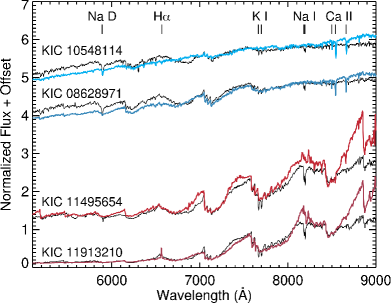
Figure 5: Four giant stars identified in our data (in color), corresponding to two early and two late-type M giants. We plot an M dwarf of similar spectral class (black) to show differences in spectral features. Prominent spectral lines used to delineate dwarf and giant spectra are identified at the top of the plot.

4.2 Binaries

Within the Kepler data, 2,909 eclipsing binaries have been identified, which is $\sim$1.5% of the nearly 200,000 Kepler stars observed (Kirk et al., 2016; Abdul-Masih et al., 2016). Two of our targets are eclipsing binaries, KIC 07174349 and KIC 10002261, which we spectral type as M4 V and M3.5 V, respectively.

Our spectra are not high enough resolution to be able to detect single- and double-lined spectroscopic binaries, however, we identify four targets which are potential white dwarf-M dwarf binaries. The spectra of KIC 07983929, KIC 09713959, KIC 09772829, and KIC 10064337 have excess flux toward blue wavelengths (Figure 6), which we attribute to a companion. Additionally, these spectra have similar spectral shapes to red-optical spectra of white dwarf–M dwarf binaries in the literature (e.g., Ren et al., 2014; Skinner et al., 2017). It is possible that the excess blue flux could be due to either improper flux calibration, slit losses, or atmospheric dispersion. Since all these binary candidates were observed using Hydra, we checked the spectra of other M dwarfs observed at the same time in the same field configuration and find no excess blue flux in these targets. Additionally, none of these targets were observed with the same fiber, and other targets observed with the same fiber in a different fiber configuration do not exhibit excess blue flux. We recommend additional spectroscopic observations of these targets at red and blue wavelengths to check that these effects are not from instrument systematics, and to confirm our assessment that these systems are likely white dwarf-M dwarf binaries. Wang et al. (2014) and Kraus et al. (2016) find that close binary companions appear to suppress planet formation, and hence decrease planet occurrence rates for these systems. As such, we remove the eclipsing and candidate white dwarf-M dwarf binaries from our analysis of planet occurrence rates, reducing our sample to 551 stars.

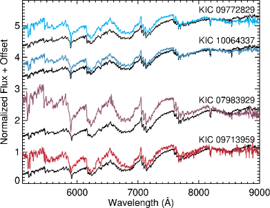
Figure 6: Four potential white dwarf-M dwarf binaries. KIC 09772829 and KIC 100064337 are compared an M2 V spectrum, and KIC 07983929 and KIC 09713959 are compared to an M3 V spectrum (black). Spectra are normalized to 8,350 Å.

4.3 Gaia Color Cuts and Binaries

We identify 61 targets with more than one source within 4″ of the KIC coordinates, in which case we choose the target with the smallest difference in $G-Kp$ magnitudes. We also check if the $M_{K_{s}}$ magnitudes (Section 3.1) are in the range we expect for an M dwarf ($4.6\lesssim M_{K_{s}}\lesssim 9.8$; M15). Four targets for which we do not have spectra (KIC 10711066, KIC 10473048, KIC 06757650, and KIC 06029053) have Gaia coordinates $<0\farcs 4$ from the KIC coordinates, but have $M_{K_{s}}$ magnitudes of 2.0, -1.6, -3.7, and 3.2, respectively. We discard these four sources from our analysis as they are likely non-M dwarfs, reducing our sample to 547 stars. Two spectroscopically observed targets, KIC 04545041 (M3.5 V) and KIC 03631048 (M4 V) have $M_{K_{s}}$ of 4.06 and 4.45, respectively. Additionally, two photometrically classified targets, KIC 11196417 (M5 V) and KIC 10991155 (M4 V), have $M_{K_{s}}$ of 4.53 and 4.56, respectively. For these four targets, we use their effective temperatures to determine radius since the $M_{K_{s}}$ vs. $R_{\star}$ relationships do not extend to $M_{K_{s}}<4.6$.

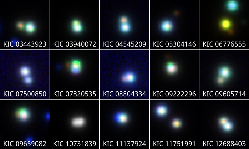
Figure 7: Probable binary stars sharing common proper motions and distances in the Gaia data. These 10″ cutouts are stacked $g$, $i$, and $y$-band images from Pan-STARRS and are centered on the target coordinates from the NASA Exoplanet Archive. The image for KIC 10731839 is only $g$-band since it is saturated in the other filters.

Within the Gaia data, 15 targets have a nearby star with a similar distance and common proper motion, which we identify as probable binaries. In Figure 7 we show 10″ cutout images of these 15 targets from the Panoramic Survey Telescope and Rapid Response System survey (Pan-STARRS, Chambers et al., 2016). We do not discard these stars in our analysis, since we use the $G-Kp$ color selection to identify our primary targets. In total, we have identified 21 binaries and binary candidates, which is 3.65% of our total sample. Duchêne & Kraus (2013) report a decreasing stellar multiplicity frequency with decreasing stellar mass, and estimate that $26\pm 3\%$ of M dwarfs are in multiple systems. Winters et al. (2019) find an M dwarf multiplicity of $26.8\pm 1.4\%$, and also note that lower mass M dwarfs have fewer companions than higher mass M dwarfs. We recognize that there are likely more unresolved binaries in our sample since we detect a $\sim$4% binary fraction, much lower than the expected $\sim$27%, however, the assessment of the effect of binaries on planet occurrence rates is beyond the scope of this paper.

5 Mid-Type M Dwarf Planets

With our updated stellar properties in hand, we now turn to planets around mid-type M dwarfs. In our Kepler star sample, there are six planet systems containing 12 confirmed planets. We also include Kepler-1650 b, for which the host star has an $r-J$ color of 3.167, just missing our color cut. Muirhead et al. (2014) identify Kepler-1650 as an M3 V star from $H$ and $K$-band spectra. Our optical spectrum of this target gives us a classification of M3.5 V. Spectra for all planet host stars are shown in Figure 8.

Additionally, there are four Kepler Objects of Interest (KOI) within our sample: KOI-959, KOI-5237, KOI-6705, and KOI-8012. Based on our spectra, KOI-959 (KIC 10002261), KOI-5327 (KIC 06776555), KOI-8012 (KIC 10452252) have spectral types of M3.5 V, M4 V, and M5 V, respectively. Using the spectral index typing system of Lépine et al. (2013), Gaidos et al. (2016a) report KOI-6705 (KIC 06423922) to be an M3.4 V star from a SNIFS optical spectrum.

Figure 8: (a) Planet host spectra for Kepler mid-type M dwarfs, ordered by spectral type from M3 V (top) to M5 V (bottom). These are the first published optical spectra for Kepler-1646 (M4 Ve) and Kepler-1582 (M5 V). (b) Orbital period versus planet radius for Kepler mid-type M dwarfs. The planet radii have been updated using our new stellar radius measurements. The radii of Earth and Mars are shown for reference.

Slawson et al. (2011) identify KOI-959 to be an eclipsing binary, which makes this planet candidate an astrophysical false positive. Additionally, Furlan et al. (2017) and Ziegler et al. (2018) find a nearby companion to KOI-959 at a separation of $\sim$0$\farcs 77$ using adaptive optics imaging. KOI-5327 is associated with three nearby companions at separations of $1\farcs 88$, $3\farcs 63$, and $3\farcs 96$ (Ziegler et al., 2017; Furlan et al., 2017). The Kepler pipeline data validation report for this system shows an out-of-transit centroid offset of $2\farcs 09$ (6.3$\sigma$), which might be due to the closest companion star. It is unclear which star the planet orbits, so we do not include this system in our analysis. Gaidos et al. (2016a) identify KOI-6705.01 as a likely false positive due to charge transfer inefficiency in a detector column on which a nearby eclipsing binary falls. Thompson et al. (2018) identify KOI-8012.01 as a Mercury-sized planet candidate in the habitable zone of its host star. Our reassessment of the radius of KOI-8012 places it at $0.43\,R_{\odot}$, which in turn increases the planet candidate radius to $0.83\,R_{\oplus}$. We do not include this planet candidate in our analysis since the system parameters (e.g., period, semi-major axis) do not have reported uncertainties, which makes accurate analysis of this system difficult. Additionally, the Kepler light curve for KOI-8012 shows significant variability and extreme flare activity, which suggests that any planet candidates around this star could be astrophysical false positives.

Table 2 and Figure 8 show the confirmed planets around mid-type M dwarfs in the Kepler field. We note that all these planets are smaller than Neptune ($3.865\,R_{\oplus}$) and have orbital periods shorter than 10 days. We update the planet parameters for all these systems based on our stellar radius and mass measurements, and compute insolation flux $S_{p}$ using:

$$\Bigg{(}\frac{S_{p}}{S_{\oplus}}\Bigg{)}=\Bigg{(}\frac{L_{\star}}{L_{\odot}}\Bigg{)}\Bigg{(}\frac{AU}{a}\Bigg{)}^{2},$$ (4)

where $(L_{\star}/L_{\odot})=(R_{\star}/R_{\odot})^{2}(T_{\mathrm{eff}}/T_{\odot})^{4}$ is the stellar luminosity, and $a$ is the semi-major axis in AU, computed from Kepler’s third law using planet orbital period from the literature and our stellar masses. The planet with the lowest stellar irradiance in our sample is Kepler-1649 b, an Earth-sized planet ($R_{p}=0.985\pm 0.054\,R_{\oplus}$) receiving nearly twice the stellar irradiation as Earth. The habitable zone definitions of Kopparapu et al. (2013) place this planet above the maximum greenhouse stellar irradiance limit.

6 Planet Occurrence Rate

With our updated stellar properties of 547 stars and a population of 13 planets around mid-type M dwarfs, we now have the critical pieces necessary to compute planet occurrence rates. We adopt the grid-based method (e.g, Howard et al., 2012; Dressing & Charbonneau, 2013; Petigura et al., 2013) to compute planet occurrence rates, $f(R_{p},P)$, which is the fraction of stars in a population (e.g., mid-type M dwarfs) that have planets with specific radii $R_{p}$ and orbital periods $P$. Using the population of known planets around Kepler mid-type M dwarfs, we count the number of Kepler mid-type M dwarfs $N_{\star,i}$ around which the $i^{th}$ known planet could have been detected with sufficient photometric precision if it was at a transiting orbital inclination:

$$f(R_{p},P)=\sum_{i=1}^{N_{p}}\frac{1/p_{i}}{N_{\star,i}},$$ (5)

where the sum is over the number of known planets $N_{p}$ from the Kepler data within the specified planet radius and orbital period range. The probability $p$ that planet $i$ is in a transiting geometry, is defined as:

$$p_{i}=\Bigg{(}\frac{R_{\star,i}+R_{p}}{a_{i}}\Bigg{)}\Bigg{(}\frac{1+e_{i}\sin\omega_{i}}{1-e_{i}^{2}}\Bigg{)},$$ (6)

where $a_{i}$ is the semi-major axis of planet $i$, $e_{i}$ is the eccentricity, and $\omega_{i}$ is the longitude of periastron (Winn, 2010; Stevens & Gaudi, 2013). Typically, $R_{p}\ll R_{\star}$ and small planets on close-in orbits are nearly circular, which makes $p_{i}\approx R_{\star,i}/a_{i}$. However, an Earth-sized planet around a mid-type M dwarf is between 2.5 and 7.5% of its host star diameter, which can have a small effect on the transit probability. Assuming circular orbits, we use:

$$p_{i}=\Bigg{(}\frac{R_{\star,i}+R_{p}}{a_{i}}\Bigg{)}.$$ (7)

We compute $N_{\star,i}$ from the number of stars for which the S/N from the Kepler photometry is high enough that a known planet could be detected. The S/N is calculated by:

$$\text{S/N}=\frac{R^{2}_{\text{p}}/R^{2}_{\star}}{\text{CDPP}_{\text{eff}}}\sqrt{\frac{t_{\text{obs}}}{P}},$$ (8)

where $\text{CDPP}_{\text{eff}}$ is the Combined Differential Photometric Precision over the duration of the transit, $t_{\text{obs}}$ is the total time spent observing the star with Kepler, and $P$ is the known planet orbital period (Muirhead et al., 2015). $\text{CDPP}_{\text{eff}}$, more precisely, is an estimate of white noise during a specific transit duration (Christiansen et al., 2012). For each star, we fit a power law to the CDPP values versus time for transits between 1.5 and 15 hours, and use this fit to determine $\text{CDPP}_{\text{eff}}$ for each planet transit duration, $t_{\mathrm{dur}}$. We compute $t_{\mathrm{dur}}$ for known planets using:

$$t_{\mathrm{dur}}=\frac{P}{\pi}\sin^{-1}\Bigg{(}\frac{\sqrt{(R_{\star}+R_{p})^{2}-(bR_{\star})^{2}}}{a}\Bigg{)},$$ (9)

where $b=a\cos\theta/R_{\star}$ is the impact parameter with orbital inclination angle $\theta$.

We use the linear ramp detection efficiency model from Mulders et al. (2015a), which was adapted from Fressin et al. (2013), where detection efficiency $f_{\mathrm{eff}}=0$ for S/N $\leq$ 6, $f_{\mathrm{eff}}=1$ for S/N $>$ 12, and $f_{\mathrm{eff}}=(\mathrm{S/N}-6)/6$ for 6 $<$ S/N $\leq$ 12. The sum of the detection efficiencies, rounded to the nearest integer, then becomes $N_{\star,i}$.

Our stellar selection criteria were chosen to isolate stars with a spectral type of M3 V and beyond, though we observed 40 stars with earlier spectral types. In our planet sample, we have identified the Kepler planets around M3 V to M5 V stars. For our planet occurrence rate calculations, we only consider the stars in this spectral type range.

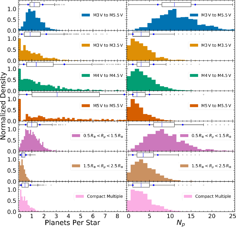
Figure 9: (Left) Planet occurrence rate distributions from our Monte Carlo analysis for different spectral type bins, planet radius bins, and for compact multiple systems. Above each distribution we give the corresponding box-and-whisker plot, which show the quartiles of each distribution. The 16^th and 84^th percentiles are shown as blue circles, and any outliers beyond $Q3+1.5\times IQR$ are shown as open circles. The M5 V upper whisker extends to $\sim$15, however, we restrict the horizontal range to just beyond the 84^th percentile of the M5 V distribution for clarity in the other plots. All of these plots are normalized such that the peak of each distribution is equal to one. (Right) Planet detection distributions from the planet occurrence rate Monte Carlo analysis and corresponding box-and-whisker plots.

6.1 Monte Carlo Analysis

The measured star and planet parameters found in Equations 7, 8, and 9 have uncertainties which contribute to the total uncertainty of the planet occurrence rate calculation. There is also spectral type uncertainty, which can move stars, including planet hosts, into or out of a spectral type bin. Additionally, due to our small planet sample size, we need to account for counting errors. In order to address these uncertainties we perform the following MC analysis. First, we address the $\pm 1$ spectral type uncertainty by drawing a random number from a uniform distribution between -1 and 1 for each star in our sample and add those numbers to each spectral type. Second, we draw a number of planet detections $N_{p}$ from a Poisson distribution with an expectation value ($\lambda$) equal to the detected planet sample size, similar to the method used in Silburt et al. (2015) and Gaidos et al. (2016b). For example, our total Kepler mid-type M dwarf planet sample size is 13, so we randomly draw a number from a Poisson distribution with $\lambda=13$, then sample with replacement that number of planets from our mid-type M dwarf planet catalog to run the occurrence rate calculations. Next, for each parameter with an uncertainty measurement in Equations 7, 8, and 9, we generate $10^{4}$ random samples from a Gaussian distribution and perform each calculation with these distributions. We also account for the effect of transit duration on S/N by assigning a random inclination angle to compute the impact parameter in Equation 9. We then run the results through Equation 5, and repeat this procedure $10^{3}$ times for seven different bins: all mid-type M dwarfs (M3 V to M5.5 V), individual spectral types (M3 V to M3.5 V, M4 V to M4.5 V, and M5 V to M5.5 V), Earth-sized planets ($0.5\,R_{\oplus}<R_{p}<1.5\,R_{\oplus}$), super-Earths ($1.5\,R_{\oplus}<R_{p}<2.5\,R_{\oplus}$), and compact multiples.

The resulting planet occurrence rates and planet detection distributions are shown in Figure 9. The occurrence rate distributions all exhibit positive skew, highlighted by the box-and-whisker plots above each distribution. Due to our random selection of $N_{p}$ from a Poisson distribution, an outcome of zero planets is possible, which results in a planet occurrence rate of zero. For our seven different bins, those with a smaller initial sample of planets are more likely to randomly draw zero planets. This effect is most prominent for the individual spectral type bins, which have prominent peaks at zero for the planet occurrence rate. Even though the $N_{p}$ distributions have a non-zero median, drawing zero planets will always result in an occurrence rate of zero, whereas drawing one or more planets can result in a different planet occurrence rate depending on the transit probability of the randomly selected planets and number of stars from the MC calculation, effectively smoothing out other peaks. We report the results from the planet occurrence rate calculation in Table 1.

Table 1: Planet occurrence rates per spectral type, planet radius, and compact multiples for mid-type M dwarfs.

Range	Planets per star	$N_{p}$	$N_{\star,i}$
M3 V to M5.5 V	$1.19^{+0.70}_{-0.49}$	$11^{+5}_{-4}$	$412^{+8}_{-8}$
M3 V to M3.5 V	$0.86^{+1.32}_{-0.68}$	$3^{+3}_{-2}$	$95^{+8}_{-8}$
M4 V to M4.5 V	$1.36^{+2.30}_{-1.02}$	$3^{+3}_{-2}$	$92^{+9}_{-8}$
M5 V to M5.5 V	$3.07^{+5.49}_{-2.49}$	$2^{+3}_{-1}$	$37^{+5}_{-6}$
$0.5\,R_{\oplus}<R_{p}<1.5\,R_{\oplus}$	$0.99^{+0.66}_{-0.50}$	$8^{+5}_{-3}$	$412^{+8}_{-9}$
$1.5\,R_{\oplus}<R_{p}<2.5\,R_{\oplus}$	$0.27^{+0.25}_{-0.18}$	$4^{+3}_{-3}$	$412^{+7}_{-9}$
Compact Multiple	$0.44^{+0.45}_{-0.33}$	$3^{+3}_{-2}$	$411^{+8}_{-8}$

Note. — We report the median, 16^th, and 84^th percentiles of each distribution from $10^{3}$ Monte Carlo trials.

7 Discussion

For early-type M dwarfs with orbital periods between 0.5 and 10 days and planets with $0.5\,R_{\oplus}<R_{p}<2.5\,R_{\oplus}$, DC15 derive a planet occurrence rate of $0.63^{+0.08}_{-0.06}$ planets per star. Similarly, Mulders et al. (2015b) compute a planet occurrence rate for M dwarfs in this range to be 0.53 planets per star. Our total occurrence rate for mid-type M dwarfs is approximately double that of DC15 and Mulders et al. (2015b) for early-type M dwarfs. We show a comparison of occurrence rates from our MC analysis to values from DC15 and Mulders et al. (2015b) in Figure 10. We also include in this figure the planet occurrence rates for stars of each spectral type F, G, and K from Mulders et al. (2015b). There is a clear trend of increasing planet occurrence toward later spectral types. If we take the median values of planet occurrence rates from our MC analysis, this suggests an increasing trend of small planets at short orbital periods toward later-type M dwarfs. We also find that a typical mid-type M dwarf will host a short period Earth-sized planet ($0.5\,R_{\oplus}<R_{p}<1.5\,R_{\oplus}$), and larger planets are about four times less common.

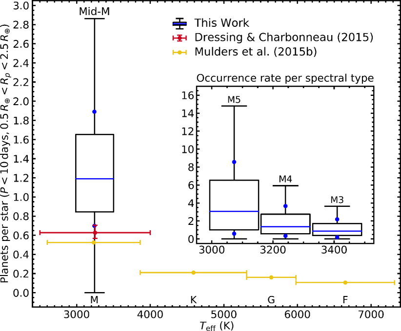
Figure 10: Planet occurrence rate as a function of stellar effective temperature for planets with orbital periods shorter than 10 days and radii between 0.5 and $2.5\,R_{\oplus}$. The measurements from our Monte Carlo analysis are shown as box-and-whisker plots (see Figure 9), where the blue line indicates the median value, the blue dots are the 16^th and 84^th percentiles of the distributions, and the box width corresponds to the temperature uncertainty. The inset plot shows the planet occurrence rates for M3 V, M4 V, and M5 V, which show evidence for an increase of planet occurrence toward later M dwarfs.

We revise the planet occurrence rate for compact multiples around mid-type M dwarfs to be $0.44^{+0.45}_{-0.33}$. This value is computed following the same MC procedure, but only considers the detectability of the outermost planet in the multi-planet system. Our occurrence rate for compact multiples is consistent within $1\sigma$ to $0.21^{+0.07}_{-0.05}$ reported by Muirhead et al. (2015), though our median value is higher due to our revised stellar radii. Muirhead et al. (2015) assumed a uniform stellar radius of 0.2 $R_{\odot}$, the peak of the radius distribution for these stars in the Kepler Stellar Catalog. For low mass stars, Boyajian et al. (2012) found that evolutionary models, which were largely used to determine radii in the Kepler Stellar Catalog, under predict stellar radii. Our radius measurements have a median value of $0.33\,R_{\odot}$, 58% larger than the median $0.21\,R_{\odot}$ from the Kepler Stellar Catalog. The stellar radii reported in Gaidos et al. (2016b) were a significant improvement over those derived from evolutionary models, but they are still $\sim$20% smaller than our measurements (Figure 4).

Ballard & Johnson (2016) assessed planet multiplicity among Kepler M dwarfs, and found that half of these systems contain five or more co-planar planets, while the other half are either single or multiple planet systems with large mutual planet inclinations. Of the seven confirmed Kepler mid-type M dwarf planet systems, three of them contain at least three planets, whereas the other four systems contain at least one planet. It is possible that all of these systems could contain additional non-transiting planets or planets that fall below the detection threshold of Kepler. The discovery of seven Earth-sized planets around the M8 V star TRAPPIST-1 shows that planet formation occurs through the end of the main sequence (Gillon et al., 2017), and supports both the increase in planet occurrence rates toward later spectral types and the large planet multiplicity from Ballard & Johnson (2016).

Thompson et al. (2018) note that pipeline detection efficiency, astrophysical reliability, and imperfect stellar information must all be taken into account for planet occurrence rate calculations. Pipeline detection efficiency has been computed for Kepler F, G, and K stars using pixel-level and flux-level transit injection (Christiansen et al., 2016; Christiansen, 2017; Burke & Catanzarite, 2017). DC15 performed their own pipeline detection efficiency for Kepler M dwarfs by injecting transit signals into light curves for all their target stars. For planets between $1\,R_{\oplus}$ and $3\,R_{\oplus}$ at orbital periods less than 10 days, their pipeline was able to recover between 80 and 90% of the injected transit signals. For planets below $1\,R_{\oplus}$, recovery averaged 58%. Astrophysical reliability tests are used to determine whether or not an observed event is due to instrumental or stellar noise or other astrophysical events. Certain signals can mimic a planet transit (e.g., eclipsing binaries, background eclipsing binaries), so tools have been developed to automatically vet planet candidates (e.g., Robovetter, Thompson et al., 2018) and statistically validate planet candidates (e.g., vespa, Morton et al., 2016). Our work has addressed the third issue of imperfect stellar information, though we do take into account a simple linear ramp model of detection efficiency in our calculations. We also note that Silburt et al. (2015) and Gaidos et al. (2016b) caution placing planets into discrete radius and period bins because it ignores information about the underlying planet distribution and will underestimate the planet occurrence rate. With a sample of only 13 planets, however, it is difficult to determine a practical planet distribution without making some assumptions. Additionally, accounting for small planet sample size dominates the error budget for our occurrence rate calculations.

From our Kepler planet occurrence rates, we can predict the number of planets in orbital periods less than 10 days around mid-type M dwarfs in the local neighborhood. Stelzer et al. (2013) conducted a survey of UV and X-ray activity of M dwarfs within 10 parsecs of the Sun, in which they observed 159 M0 V through M8 V stars, and estimated that their volume-limited M dwarf sample was 90% complete. This sample includes 101 stars with spectral types between M3 V and M5.5 V, which means there are potentially $120^{+71}_{-49}$ small, short period planets around these nearby stars. So far, there have been 20 planets found around 9 of these nearby mid-type M dwarfs, all discovered via the radial velocity technique. Of those 20 planets, 10 have orbital periods shorter than 10 days. The faintest mid-type M dwarf around which a planet has been detected using the radial velocity technique has a $V$-band magnitude of 12.22 (GJ 3323), and the smallest radial velocity amplitude for a planet detected around these stars is $1.06\pm 0.15\,\mathrm{m\,s}^{-1}$ (GJ 273 c, Astudillo-Defru et al., 2017). There are 51 nearby mid-type M dwarfs with $V$-band magnitudes less than 12.22. Our planet occurrence rates suggest there are $61^{+35}_{-25}$ small, short period planets around these stars. Since 10 of these planets have already been found, there may be around 50 additional planets orbiting nearby mid-type M dwarfs which could be detected with current radial velocity instruments (e.g., HARPS, Pepe et al., 2011), assuming the planets are massive enough to induce a $1\,\mathrm{m\,s}^{-1}$ signal. NEID and EXPRES aim to achieve even greater precision below $30\,\mathrm{cm\,s}^{-1}$ at optical wavelengths (Halverson et al., 2016; Jurgenson et al., 2016). The Habitable Zone Planet Finder (HPF; Mahadevan et al., 2012) will specifically target mid- to late-type M dwarfs at near-infrared wavelengths, with a goal of $1\,\mathrm{m\,s}^{-1}$ precision. Recent commissioning observations with HPF have already achieved $1.3\,\mathrm{m\,s}^{-1}$ precision on Barnard’s Star (Mahadevan et al., 2018).

Since the original Kepler mission was designed to detect Earth-like planets around Sun-like stars, less emphasis was placed on low-mass stars. The K2 mission (Howell et al., 2014), however, was well suited for detecting planets around the latest type stars along the ecliptic plane, and has already produced dozens of confirmed and candidate planets around M dwarfs, opening up another rich data set to expand this planet occurrence rate study. The K2 M Dwarf Project (PIs Schleider, J.; Crossfield, I.; Dressing, C.) alone has over 25,000 targets in K2 Campaigns 4 through 19, about five times larger than the number of M dwarfs observed with Kepler. The ground based survey MEarth (Nutzman & Charbonneau, 2008) is surveying M dwarfs for planets, and the Search for habitable Planets EClipsing ULtra-cOOl Stars (SPECULOOS; Burdanov et al., 2017) is starting to search for planets around 1,000 late-type M dwarfs and brown dwarfs. Since small, short period planets are more prevalent around smaller stars, these surveys should be fruitful. The recently launched TESS mission is also expected to find 500 to 1,000 planets around bright M dwarfs across the entire night sky (Barclay et al., 2018; Ballard, 2018). Barclay et al. (2018) predicted that 54 planets will be found with orbital periods less than 10 days around bright ($K_{S}<10$) mid-type M dwarfs, assuming the occurrence rates of DC15. Based on our occurrence rates, we expect a more optimistic TESS yield of $\sim$100 planets around bright mid-type M dwarfs.

8 Acknowledgements

We would like to thank WIYN observing assistants Amy Robertson, Anthony Paat, Christian Soto, Dave Summers, Doug Williams, Karen Butler, and Malanka Riabokin, DCT telescope operators Andrew Hayslip, Heidi Larson, Jason Sanborn, and Teznie Pugh, and IRTF telescope operators Brian Cabreira, Dave Griep, Eric Volquardsen, Greg Osterman, and Tony Matulonis. We would also like to thank NOAO observing support scientists Daryl Willmarth, Dianne Harmer, Mark Everett, and Susan Ridgway. K. Hardegree-Ullman would like to thank Adam Schneider and Wayne Oswald for conducting some of the observations herein at the DCT and WIYN, and Courtney Dressing, Gijs Mulders, and Jon Zink for informative discussions regarding planet occurrence rates and statistics.

Data presented herein were obtained at the WIYN Observatory from telescope time allocated to NN-EXPLORE through the scientific partnership of the National Aeronautics and Space Administration, the National Science Foundation, and the National Optical Astronomy Observatory. This work was supported by a NASA WIYN PI Data Award, administered by the NASA Exoplanet Science Institute.

These results made use of the Discovery Channel Telescope at Lowell Observatory. Lowell is a private, non-profit institution dedicated to astrophysical research and public appreciation of astronomy and operates the DCT in partnership with Boston University, the University of Maryland, the University of Toledo, Northern Arizona University and Yale University. The upgrade of the DeVeny optical spectrograph has been funded by a generous grant from John and Ginger Giovale.

Guoshoujing Telescope (the Large Sky Area Multi-Object Fiber Spectroscopic Telescope LAMOST) is a National Major Scientific Project built by the Chinese Academy of Sciences. Funding for the project has been provided by the National Development and Reform Commission. LAMOST is operated and managed by the National Astronomical Observatories, Chinese Academy of Sciences.

This research has made use of the NASA Exoplanet Archive, which is operated by the California Institute of Technology, under contract with the National Aeronautics and Space Administration under the Exoplanet Exploration Program.

This work has made use of data from the European Space Agency (ESA) mission Gaia (https://www.cosmos.esa.int/gaia), processed by the Gaia Data Processing and Analysis Consortium (DPAC, https://www.cosmos.esa.int/web/gaia/dpac/consortium). Funding for the DPAC has been provided by national institutions, in particular the institutions participating in the Gaia Multilateral Agreement.

This work made use of the gaia-kepler.fun crossmatch database created by Megan Bedell.

The Pan-STARRS1 Surveys (PS1) and the PS1 public science archive have been made possible through contributions by the Institute for Astronomy, the University of Hawaii, the Pan-STARRS Project Office, the Max-Planck Society and its participating institutes, the Max Planck Institute for Astronomy, Heidelberg and the Max Planck Institute for Extraterrestrial Physics, Garching, The Johns Hopkins University, Durham University, the University of Edinburgh, the Queen’s University Belfast, the Harvard-Smithsonian Center for Astrophysics, the Las Cumbres Observatory Global Telescope Network Incorporated, the National Central University of Taiwan, the Space Telescope Science Institute, the National Aeronautics and Space Administration under Grant No. NNX08AR22G issued through the Planetary Science Division of the NASA Science Mission Directorate, the National Science Foundation Grant No. AST-1238877, the University of Maryland, Eotvos Lorand University (ELTE), the Los Alamos National Laboratory, and the Gordon and Betty Moore Foundation.

The authors wish to recognize and acknowledge the very significant cultural role and reverence that the summit of Maunakea has always had within the indigenous Hawaiian community. We are most fortunate to have the opportunity to conduct observations from this mountain.

=2in

Table 2: Kepler Mid-Type M Dwarf Planets

Planet Name	Host Type	$R_{\star}$	$R_{p}$	$a/R_{\star}$	Period	$t_{\mathrm{dur}}$	Transit	$S_{p}$	References
	(This Work)	($R_{\odot}$)	($R_{\oplus}$)		(days)	(hours)	Probability	($S_{\oplus}$)
Kepler-42 b	M3 V	$0.174\pm 0.005$	$0.757\pm 0.025$	$14.46^{+0.43}_{-0.40}$	$1.2137706\pm 2.4$$\times$$10^{-7}$	$0.57\pm 0.04$	$0.0719\pm 0.0021$	$26.86^{+3.31}_{-3.08}$	2
Kepler-42 c			$0.727\pm 0.023$	$7.49^{+0.23}_{-0.21}$	$0.45328731\pm 5.0$$\times$$10^{-8}$	$0.44\pm 0.03$	$0.1385\pm 0.0041$	$99.78^{+12.16}_{-11.26}$	2
Kepler-42 d			$0.662\pm 0.032$	$19.26^{+0.59}_{-0.54}$	$1.86511236\pm 7.3$$\times$$10^{-7}$	$0.56\pm 0.09$	$0.0537\pm 0.0016$	$15.13^{+1.88}_{-1.75}$	2
Kepler-1650 b	M3.5 V	$0.364\pm 0.010$	$1.044\pm 0.042$	$10.88^{+0.34}_{-0.31}$	$1.53818001\pm 1.5$$\times$$10^{-6}$	$1.05\pm 0.11$	$0.0942\pm 0.0028$	$42.67^{+5.59}_{-4.88}$	2
Kepler-1646 b	M4 Ve	$0.374\pm 0.011$	$1.809\pm 0.129$	$21.86^{+0.71}_{-0.65}$	$4.48558383\pm 1.1$$\times$$10^{-5}$	$1.53\pm 0.07$	$0.0478\pm 0.0015$	$9.57^{+1.29}_{-1.11}$	3
Kepler-446 b	M4 V	$0.217\pm 0.006$	$1.357\pm 0.073$	$14.94^{+0.46}_{-0.44}$	$1.565409\pm 3.3$$\times$$10^{-6}$	$0.67\pm 0.09$	$0.0708\pm 0.0022$	$20.62^{+2.62}_{-2.50}$	4
Kepler-446 c			$1.003\pm 0.051$	$23.23^{+0.71}_{-0.68}$	$3.036179\pm 5.5$$\times$$10^{-6}$	$0.96\pm 0.10$	$0.0449\pm 0.0014$	$8.47^{+1.11}_{-1.00}$	4
Kepler-446 d			$1.227\pm 0.063$	$33.02^{+1.03}_{-0.95}$	$5.148921\pm 2.2$$\times$$10^{-5}$	$0.93\pm 0.13$	$0.0318\pm 0.0010$	$4.18^{+0.56}_{-0.49}$	4
Kepler-445 b	M4.5 V	$0.305\pm 0.009$	$1.519\pm 0.079$	$18.63^{+0.59}_{-0.57}$	$2.9841664\pm 9.1$$\times$$10^{-6}$	$1.27\pm 0.04$	$0.0561\pm 0.0018$	$11.87^{+1.62}_{-1.43}$	2, 4
Kepler-445 c			$2.390\pm 0.092$	$25.82^{+0.83}_{-0.79}$	$4.87122714\pm 6.3$$\times$$10^{-6}$	$1.54\pm 0.05$	$0.0415\pm 0.0013$	$6.17^{+0.83}_{-0.73}$	2, 4
Kepler-445 d			$1.167\pm 0.098$	$36.38^{+1.17}_{-1.10}$	$8.15272856\pm 6.7$$\times$$10^{-5}$	$1.75\pm 0.06$	$0.0284\pm 0.0009$	$3.11^{+0.42}_{-0.38}$	2, 4
Kepler-1649 b	M5 V	$0.231\pm 0.007$	$0.985\pm 0.054$	$45.02^{+1.42}_{-1.36}$	$8.68909\pm 2.4$$\times$$10^{-5}$	$1.38\pm 0.27$	$0.0231\pm 0.0007$	$1.82^{+0.25}_{-0.23}$	1
Kepler-1582 b	M5 V	$0.217\pm 0.006$	$1.060\pm 0.071$	$31.41^{+0.96}_{-0.94}$	$4.838177\pm 8.8$$\times$$10^{-5}$	$1.23\pm 0.04$	$0.0333\pm 0.0010$	$3.75^{+0.50}_{-0.46}$	3

Note. — References: (1) Angelo et al. (2017), (2) Mann et al. (2017), (3) Morton et al. (2016), (4) Muirhead et al. (2015)

Table 3: Stellar parameters for spectroscopically classified targets.

KIC ID	Distance	$M_{K_{S}}$	Telescopea	Spec. Typeb	$T_{\mathrm{eff}}$c	[Fe/H]	$R_{\star}$	$M_{\star}$
	(pc)	(mag)			(K)	(dex)	($R_{\odot}$)	($M_{\odot}$)
01995305	$139.882\pm 1.253$	$6.784\pm 0.039$	W/I	M3.5 V	3325	$-0.426\pm 0.100$	$0.331\pm 0.010$	$0.320\pm 0.010$
02164791	$\cdots$	$\cdots$	D/I	M4.5 Ve	3157	$-0.166\pm 0.099$	$0.218\pm 0.044$	$0.182\pm 0.064$
02283749	$291.795\pm 6.182$	$5.546\pm 0.053$	W	M4 Ve	3241	$\cdots$	$0.516\pm 0.017$	$0.518\pm 0.015$
02693779	$176.658\pm 1.632$	$6.308\pm 0.038$	W	M4 V	3241	$\cdots$	$0.399\pm 0.013$	$0.394\pm 0.011$
02832720	$106.036\pm 5.989$	$6.352\pm 0.125$	W/I	M4 Ve	3241	$0.284\pm 0.152$	$0.398\pm 0.020$	$0.386\pm 0.022$
02834637	$125.012\pm 0.700$	$6.406\pm 0.023$	W/I	M4 Ve	3241	$0.063\pm 0.073$	$0.387\pm 0.011$	$0.378\pm 0.009$
03219046	$63.177\pm 0.308$	$8.621\pm 0.026$	W	M5 Ve	3073	$\cdots$	$0.166\pm 0.005$	$0.134\pm 0.003$
03232191	$\cdots$	$\cdots$	W	M4 V	3241	$\cdots$	$0.258\pm 0.053$	$0.226\pm 0.075$
03330684	$\cdots$	$\cdots$	W	M7 V	2736	$\cdots$	$0.126\pm 0.018$	$0.091\pm 0.018$
03340246	$112.936\pm 0.784$	$7.414\pm 0.027$	W	M4 V	3241	$\cdots$	$0.265\pm 0.008$	$0.236\pm 0.006$
03453233	$193.017\pm 4.811$	$7.819\pm 0.094$	D	M4 V	3241	$\cdots$	$0.226\pm 0.011$	$0.194\pm 0.010$
03561148	$59.378\pm 0.128$	$6.319\pm 0.015$	L	M4 V	3241	$\cdots$	$0.398\pm 0.012$	$0.392\pm 0.009$
03629595	$116.233\pm 0.590$	$7.001\pm 0.027$	W/I	M4 V	3241	$-0.070\pm 0.101$	$0.310\pm 0.009$	$0.289\pm 0.007$
03631048	$351.484\pm 4.550$	$4.449\pm 0.033$	W/I	M4 Ve	3241	$0.118\pm 0.059$	$0.286\pm 0.054$	$0.260\pm 0.082$
03642851	$200.723\pm 2.401$	$6.322\pm 0.038$	W	M4 V	3241	$\cdots$	$0.398\pm 0.013$	$0.391\pm 0.011$
03654827	$94.367\pm 0.753$	$6.884\pm 0.027$	W	M6 V	2904	$\cdots$	$0.325\pm 0.010$	$0.305\pm 0.008$
03731321	$86.438\pm 0.375$	$7.493\pm 0.022$	I	M3.5 V	3325	$0.044\pm 0.091$	$0.259\pm 0.007$	$0.227\pm 0.006$
03940072	$107.897\pm 5.365$	$5.541\pm 0.110$	W/I	M5 V	3073	$-0.066\pm 0.097$	$0.514\pm 0.023$	$0.519\pm 0.021$
03941669	$117.196\pm 0.621$	$6.969\pm 0.026$	W/I	M4.5 V	3157	$0.132\pm 0.075$	$0.317\pm 0.009$	$0.293\pm 0.008$
03954332	$150.850\pm 2.368$	$7.894\pm 0.065$	D	M5 V	3073	$\cdots$	$0.220\pm 0.008$	$0.187\pm 0.007$
04078409	$76.338\pm 0.596$	$8.739\pm 0.037$	D	M6 V	2904	$\cdots$	$0.158\pm 0.005$	$0.128\pm 0.003$
04248433	$36.985\pm 0.072$	$7.593\pm 0.018$	W/I	M5.5 Ve	2989	$0.296\pm 0.075$	$0.252\pm 0.007$	$0.216\pm 0.006$
04270856	$151.141\pm 2.118$	$6.432\pm 0.042$	W	M2.5 V	3494	$\cdots$	$0.382\pm 0.012$	$0.374\pm 0.011$
04448009	$239.205\pm 4.375$	$6.246\pm 0.050$	W	M4 V	3241	$\cdots$	$0.409\pm 0.014$	$0.404\pm 0.012$
04470937	$17.448\pm 0.033$	$6.131\pm 0.017$	W	M2 V	3578	$\cdots$	$0.425\pm 0.013$	$0.423\pm 0.010$
04545041	$410.440\pm 23.898$	$4.064\pm 0.130$	W/I	M3.5 Ve	3325	$0.424\pm 0.110$	$0.357\pm 0.069$	$0.364\pm 0.108$
04545209	$175.733\pm 2.422$	$6.146\pm 0.039$	W	M4 V	3241	$\cdots$	$0.423\pm 0.013$	$0.420\pm 0.011$
04568065	$82.102\pm 0.425$	$6.941\pm 0.023$	W	M5 V	3073	$\cdots$	$0.318\pm 0.010$	$0.297\pm 0.007$
04726552	$157.506\pm 1.591$	$7.180\pm 0.039$	W	M4 V	3241	$\cdots$	$0.290\pm 0.009$	$0.265\pm 0.008$
04730040	$227.179\pm 4.623$	$7.371\pm 0.068$	D	M4 V	3241	$\cdots$	$0.270\pm 0.010$	$0.241\pm 0.010$
04741907	$119.957\pm 1.334$	$7.656\pm 0.037$	W	M5 V	3073	$\cdots$	$0.241\pm 0.008$	$0.210\pm 0.006$
04815654	$64.279\pm 0.356$	$8.931\pm 0.030$	D/W	M6 V	2904	$\cdots$	$0.148\pm 0.005$	$0.118\pm 0.003$
04856658	$119.571\pm 1.044$	$7.346\pm 0.032$	W	M3 V	3410	$\cdots$	$0.272\pm 0.009$	$0.244\pm 0.007$
04913121	$66.698\pm 0.471$	$8.960\pm 0.038$	D/W	M6 Ve	2904	$\cdots$	$0.146\pm 0.005$	$0.117\pm 0.003$
04917182	$91.451\pm 0.495$	$7.119\pm 0.023$	W	M5.5 V	2989	$\cdots$	$0.297\pm 0.009$	$0.273\pm 0.007$
04946433	$117.314\pm 3.026$	$4.866\pm 0.060$	W	M3.5 V	3325	$\cdots$	$0.636\pm 0.022$	$0.621\pm 0.017$
05002836	$28.142\pm 0.020$	$6.916\pm 0.017$	W/I	M4 V	3241	$-0.183\pm 0.086$	$0.319\pm 0.009$	$0.301\pm 0.007$
05079348	$76.937\pm 0.199$	$6.614\pm 0.020$	W	M3.5 V	3325	$\cdots$	$0.358\pm 0.011$	$0.345\pm 0.008$
05122206	$45.857\pm 0.080$	$6.689\pm 0.020$	W	M4.5 V	3157	$\cdots$	$0.349\pm 0.010$	$0.334\pm 0.008$
05126248	$122.180\pm 1.109$	$6.441\pm 0.028$	W	M5 V	3073	$\cdots$	$0.381\pm 0.012$	$0.372\pm 0.009$
05175854	$67.247\pm 0.371$	$8.789\pm 0.033$	D/W	M7 Ve	2736	$\cdots$	$0.156\pm 0.005$	$0.125\pm 0.003$
05181762	$206.139\pm 2.134$	$5.703\pm 0.030$	W	M4 V	3241	$\cdots$	$0.491\pm 0.015$	$0.493\pm 0.012$
05256590	$129.297\pm 1.581$	$8.145\pm 0.051$	D	M5 V	3073	$\cdots$	$0.199\pm 0.007$	$0.166\pm 0.005$
05304146	$77.219\pm 0.772$	$6.464\pm 0.030$	W	M6.5 Ve	2820	$\cdots$	$0.378\pm 0.012$	$0.369\pm 0.009$
05341486	$229.710\pm 23.293$	$5.717\pm 0.226$	W	M5.5 Ve	2989	$\cdots$	$0.488\pm 0.038$	$0.489\pm 0.038$
05353762	$54.996\pm 0.374$	$9.361\pm 0.036$	W	M7 V	2736	$\cdots$	$0.129\pm 0.004$	$0.102\pm 0.003$
05354341	$66.588\pm 0.183$	$7.420\pm 0.021$	W	M4 Ve	3241	$\cdots$	$0.265\pm 0.008$	$0.236\pm 0.006$
05438886	$157.235\pm 1.454$	$6.946\pm 0.033$	W	M4 V	3241	$\cdots$	$0.317\pm 0.010$	$0.296\pm 0.008$
05513232	$239.522\pm 3.730$	$5.296\pm 0.042$	W	M4.5 Ve	3157	$\cdots$	$0.558\pm 0.018$	$0.557\pm 0.015$
05513833	$107.660\pm 1.513$	$6.412\pm 0.037$	W	M4 V	3241	$\cdots$	$0.385\pm 0.012$	$0.377\pm 0.010$
05515259	$107.679\pm 0.724$	$7.660\pm 0.029$	W	M3 Ve	3410	$\cdots$	$0.241\pm 0.007$	$0.209\pm 0.005$
05602310	$148.886\pm 2.970$	$5.862\pm 0.047$	W/I	M4 V	3241	$-0.054\pm 0.333$	$0.463\pm 0.014$	$0.467\pm 0.013$
05603484	$108.713\pm 0.447$	$6.629\pm 0.022$	W	M4 V	3241	$\cdots$	$0.356\pm 0.011$	$0.343\pm 0.008$
05603847	$80.025\pm 0.487$	$8.491\pm 0.030$	W	M5 V	3073	$\cdots$	$0.174\pm 0.005$	$0.142\pm 0.004$
05649085	$124.787\pm 0.831$	$6.833\pm 0.029$	W	M3 Ve	3410	$\cdots$	$0.331\pm 0.010$	$0.313\pm 0.008$
05791720	$70.692\pm 0.185$	$6.185\pm 0.019$	L	M3.5 Ve	3325	$\cdots$	$0.417\pm 0.012$	$0.414\pm 0.010$
05818116	$123.847\pm 0.573$	$6.428\pm 0.025$	W	M2 V	3578	$\cdots$	$0.383\pm 0.012$	$0.374\pm 0.009$
05859112	$95.371\pm 0.430$	$7.075\pm 0.025$	W/I	M4.5 V	3157	$0.572\pm 0.101$	$0.310\pm 0.009$	$0.278\pm 0.008$
05859124	$154.233\pm 1.347$	$6.853\pm 0.033$	W	M3.5 V	3325	$\cdots$	$0.328\pm 0.010$	$0.310\pm 0.008$
05868793d	$78.891\pm 0.440$	$7.949\pm 0.026$	W	M5 V	3073	$0.120\pm 0.200$	$0.217\pm 0.006$	$0.182\pm 0.005$
05868814	$263.882\pm 5.816$	$6.214\pm 0.060$	W	M3.5 V	3325	$\cdots$	$0.413\pm 0.015$	$0.409\pm 0.013$
05943385	$42.711\pm 0.089$	$7.360\pm 0.018$	W/I	M4.5 V	3157	$0.364\pm 0.172$	$0.276\pm 0.008$	$0.242\pm 0.006$
05944764	$159.531\pm 1.214$	$6.400\pm 0.027$	W	M3.5 V	3325	$\cdots$	$0.387\pm 0.012$	$0.379\pm 0.009$
05953947	$111.177\pm 0.590$	$6.918\pm 0.025$	W/I	M4 V	3241	$-0.296\pm 0.112$	$0.317\pm 0.009$	$0.301\pm 0.008$
06037009	$133.160\pm 0.735$	$6.735\pm 0.027$	W/I	M4 Ve	3241	$-0.178\pm 0.140$	$0.340\pm 0.010$	$0.327\pm 0.009$
06102091	$136.951\pm 1.412$	$7.243\pm 0.042$	W	M4 Ve	3241	$\cdots$	$0.283\pm 0.009$	$0.257\pm 0.008$
06102845	$125.299\pm 1.256$	$7.562\pm 0.045$	W	M4 V	3241	$\cdots$	$0.251\pm 0.008$	$0.220\pm 0.007$
06117602	$20.941\pm 0.027$	$8.769\pm 0.018$	I	M5 V	3073	$-0.035\pm 0.075$	$0.157\pm 0.004$	$0.126\pm 0.003$
06183400	$74.079\pm 0.279$	$7.498\pm 0.023$	W/I	M4 V	3241	$-0.277\pm 0.098$	$0.254\pm 0.007$	$0.227\pm 0.006$
06183736	$140.704\pm 1.436$	$6.808\pm 0.040$	W/I	M4 Ve	3241	$0.180\pm 0.095$	$0.337\pm 0.010$	$0.316\pm 0.009$
06187812	$269.005\pm 3.559$	$5.038\pm 0.035$	W/I	M3 Ve	3410	$0.174\pm 0.195$	$0.607\pm 0.018$	$0.596\pm 0.016$
06214037	$218.767\pm 5.960$	$7.682\pm 0.103$	D	M4 V	3241	$\cdots$	$0.239\pm 0.012$	$0.207\pm 0.011$
06233711	$57.618\pm 0.142$	$7.717\pm 0.022$	D	M5 Ve	3073	$\cdots$	$0.236\pm 0.007$	$0.204\pm 0.005$
06264426	$150.494\pm 1.242$	$6.621\pm 0.037$	W/I	M3 V	3410	$-0.148\pm 0.067$	$0.355\pm 0.011$	$0.344\pm 0.010$
06268411	$95.286\pm 0.476$	$7.374\pm 0.023$	W/I	M2.5 V	3494	$-0.133\pm 0.105$	$0.269\pm 0.008$	$0.241\pm 0.006$
06424725	$154.652\pm 2.072$	$6.764\pm 0.038$	W	M4 V	3241	$\cdots$	$0.339\pm 0.011$	$0.323\pm 0.009$
06444896e	$92.191\pm 0.546$	$7.764\pm 0.029$	W	M5 V	3073	$-0.150\pm 0.110$	$0.231\pm 0.007$	$0.199\pm 0.005$
06471285	$\cdots$	$\cdots$	D	M5 V	3073	$\cdots$	$0.190\pm 0.040$	$0.153\pm 0.052$
06605595	$85.366\pm 0.301$	$6.337\pm 0.018$	W/I	M4 V	3241	$0.291\pm 0.083$	$0.401\pm 0.011$	$0.389\pm 0.010$
06665209	$164.525\pm 3.590$	$8.293\pm 0.082$	W	M5 V	3073	$\cdots$	$0.188\pm 0.008$	$0.155\pm 0.007$
06672297	$75.366\pm 0.294$	$7.468\pm 0.021$	W	M4 V	3241	$\cdots$	$0.260\pm 0.008$	$0.230\pm 0.006$
06676217	$149.317\pm 1.230$	$7.113\pm 0.033$	W	M4 V	3241	$\cdots$	$0.298\pm 0.009$	$0.274\pm 0.007$
06693042	$130.426\pm 1.071$	$5.818\pm 0.026$	W/I	M4 V	3241	$-0.299\pm 0.096$	$0.465\pm 0.013$	$0.474\pm 0.012$
06752213	$163.992\pm 1.565$	$7.100\pm 0.037$	W	M4 V	3241	$\cdots$	$0.299\pm 0.010$	$0.275\pm 0.008$
06761765	$142.006\pm 1.282$	$7.162\pm 0.031$	W	M4 V	3241	$\cdots$	$0.292\pm 0.009$	$0.267\pm 0.007$
06768613	$185.719\pm 3.521$	$7.525\pm 0.060$	W	M4 V	3241	$\cdots$	$0.254\pm 0.009$	$0.224\pm 0.008$
06776555	$108.690\pm 0.481$	$7.053\pm 0.031$	W/I	M4 V	3241	$-0.117\pm 0.096$	$0.304\pm 0.009$	$0.282\pm 0.008$
06783223	$89.125\pm 0.913$	$8.602\pm 0.042$	D	M7 Ve	2736	$\cdots$	$0.167\pm 0.006$	$0.135\pm 0.004$
06784339	$114.392\pm 1.100$	$8.140\pm 0.043$	D/I	M6 V	2904	$-0.074\pm 0.142$	$0.200\pm 0.006$	$0.166\pm 0.005$
06805049	$224.585\pm 3.035$	$6.025\pm 0.039$	D	M4 V	3241	$\cdots$	$0.440\pm 0.014$	$0.440\pm 0.012$
06837702	$250.199\pm 17.033$	$5.324\pm 0.148$	W	M4 Ve	3241	$\cdots$	$0.554\pm 0.030$	$0.552\pm 0.027$
06847171	$170.189\pm 1.015$	$5.795\pm 0.023$	W/I	M4 V	3241	$0.568\pm 0.087$	$0.487\pm 0.014$	$0.477\pm 0.013$
07008143	$47.933\pm 0.095$	$7.405\pm 0.012$	W	M5 V	3073	$\cdots$	$0.266\pm 0.008$	$0.237\pm 0.005$
07022137	$114.244\pm 0.582$	$6.353\pm 0.019$	W	M4 V	3241	$\cdots$	$0.393\pm 0.012$	$0.386\pm 0.009$
07091150	$124.185\pm 1.338$	$7.806\pm 0.038$	W	M4.5 V	3157	$\cdots$	$0.227\pm 0.007$	$0.195\pm 0.006$
07102366	$200.921\pm 1.978$	$6.434\pm 0.035$	W	M4 V	3241	$\cdots$	$0.382\pm 0.012$	$0.373\pm 0.010$
07102500	$152.605\pm 0.969$	$5.361\pm 0.022$	W/I	M4 Ve	3241	$0.185\pm 0.123$	$0.550\pm 0.015$	$0.547\pm 0.014$
07177371	$195.153\pm 2.322$	$6.110\pm 0.036$	W/I	M5 V	3073	$0.226\pm 0.071$	$0.432\pm 0.013$	$0.425\pm 0.012$
07185487	$245.782\pm 3.523$	$5.928\pm 0.039$	W	M4 V	3241	$\cdots$	$0.455\pm 0.014$	$0.456\pm 0.012$
07185789	$110.923\pm 0.646$	$7.008\pm 0.023$	W/I	M4 V	3241	$0.011\pm 0.070$	$0.311\pm 0.009$	$0.288\pm 0.007$
07272205	$166.472\pm 1.413$	$6.157\pm 0.026$	W	M3.5 V	3325	$\cdots$	$0.421\pm 0.013$	$0.418\pm 0.010$
07304449f	$134.397\pm 0.721$	$6.555\pm 0.024$	W	M3.5 V	3325	$-0.110\pm 0.090$	$0.364\pm 0.010$	$0.355\pm 0.009$
07341653	$19.169\pm 0.017$	$7.509\pm 0.016$	L	M5 Ve	3073	$\cdots$	$0.256\pm 0.008$	$0.226\pm 0.005$
07350067g	$127.591\pm 0.617$	$6.498\pm 0.018$	W	M4 Ve	3241	$\cdots$	$0.374\pm 0.011$	$0.363\pm 0.009$
07352892	$90.769\pm 0.461$	$7.235\pm 0.017$	W	M4.5 V	3157	$\cdots$	$0.284\pm 0.008$	$0.258\pm 0.006$
07500850	$399.363\pm 12.883$	$4.935\pm 0.074$	W	M4 Ve	3241	$\cdots$	$0.623\pm 0.023$	$0.611\pm 0.018$
07505473	$42.926\pm 0.759$	$7.737\pm 0.042$	W/I	M5 Ve	3073	$0.009\pm 0.095$	$0.235\pm 0.007$	$0.202\pm 0.006$
07505644	$293.822\pm 4.143$	$5.111\pm 0.039$	W/I	M3 Ve	3410	$0.179\pm 0.094$	$0.594\pm 0.018$	$0.585\pm 0.016$
07517730	$33.970\pm 0.078$	$8.889\pm 0.014$	W	M6 V	2904	$\cdots$	$0.150\pm 0.004$	$0.120\pm 0.003$
07582793	$189.719\pm 2.246$	$7.172\pm 0.044$	D/W	M3.5 V	3325	$\cdots$	$0.291\pm 0.010$	$0.266\pm 0.008$
07596910	$78.058\pm 0.347$	$5.968\pm 0.015$	W	M4.5 V	3157	$\cdots$	$0.449\pm 0.013$	$0.449\pm 0.010$
07659103	$93.778\pm 0.371$	$6.971\pm 0.016$	W/I	M4 V	3241	$-0.266\pm 0.094$	$0.311\pm 0.009$	$0.293\pm 0.007$
07661403	$154.592\pm 1.384$	$6.472\pm 0.023$	W	M4 Ve	3241	$\cdots$	$0.377\pm 0.011$	$0.367\pm 0.009$
07729309	$\cdots$	$\cdots$	D/I	M2 V	3578	$-0.204\pm 0.093$	$0.410\pm 0.060$	$0.405\pm 0.094$
07734382	$155.505\pm 2.173$	$7.255\pm 0.048$	W	M4 Ve	3241	$\cdots$	$0.282\pm 0.010$	$0.255\pm 0.008$
07799514	$\cdots$	$\cdots$	W	M4 V	3241	$\cdots$	$0.258\pm 0.053$	$0.226\pm 0.075$
07799844	$103.436\pm 1.095$	$8.559\pm 0.041$	D	M6 V	2904	$\cdots$	$0.169\pm 0.006$	$0.138\pm 0.004$
07809767	$204.264\pm 6.670$	$7.960\pm 0.109$	D	M5 V	3073	$\cdots$	$0.214\pm 0.011$	$0.181\pm 0.010$
07849191	$57.455\pm 0.165$	$8.308\pm 0.023$	W	M4 V	3241	$\cdots$	$0.187\pm 0.006$	$0.154\pm 0.004$
07903237	$439.487\pm 34.408$	$6.587\pm 0.173$	D	M4 Ve	3241	$\cdots$	$0.362\pm 0.025$	$0.349\pm 0.028$
07938787	$154.623\pm 1.454$	$5.562\pm 0.023$	W	M4 V	3241	$\cdots$	$0.513\pm 0.015$	$0.515\pm 0.012$
07939565	$65.472\pm 0.154$	$6.628\pm 0.012$	W	M2.5 Ve	3494	$\cdots$	$0.357\pm 0.010$	$0.343\pm 0.008$
08036551	$93.164\pm 1.147$	$8.725\pm 0.047$	D	M6 V	2904	$\cdots$	$0.159\pm 0.005$	$0.128\pm 0.004$
08040522	$253.639\pm 8.224$	$7.293\pm 0.097$	D	M4 V	3241	$\cdots$	$0.278\pm 0.013$	$0.251\pm 0.013$
08076831	$48.598\pm 0.090$	$6.944\pm 0.012$	W	M2.5 V	3494	$\cdots$	$0.317\pm 0.009$	$0.297\pm 0.007$
08082302	$157.362\pm 1.149$	$6.546\pm 0.029$	W	M4 V	3241	$\cdots$	$0.367\pm 0.011$	$0.356\pm 0.009$
08095972	$114.779\pm 0.547$	$6.773\pm 0.020$	W/I	M2 V	3578	$-0.143\pm 0.093$	$0.336\pm 0.009$	$0.321\pm 0.008$
08167877	$323.982\pm 11.181$	$6.646\pm 0.112$	W	M3 V	3410	$\cdots$	$0.354\pm 0.018$	$0.340\pm 0.019$
08190958	$47.983\pm 0.090$	$6.501\pm 0.020$	W	M3.5 V	3325	$\cdots$	$0.373\pm 0.011$	$0.363\pm 0.009$
08197652	$\cdots$	$\cdots$	W	M4 Ve	3241	$\cdots$	$0.258\pm 0.053$	$0.226\pm 0.075$
08213019	$220.989\pm 2.549$	$5.429\pm 0.029$	W	M4 V	3241	$\cdots$	$0.536\pm 0.016$	$0.537\pm 0.013$
08233951	$102.901\pm 0.504$	$6.994\pm 0.025$	W/I	M4 V	3241	$-0.332\pm 0.097$	$0.307\pm 0.009$	$0.290\pm 0.008$
08236114	$140.875\pm 1.895$	$8.403\pm 0.082$	D/W	M4 V	3241	$\cdots$	$0.180\pm 0.008$	$0.147\pm 0.006$
08278279	$183.522\pm 3.684$	$6.100\pm 0.047$	W/I	M6 Ve	2904	$0.530\pm 0.062$	$0.439\pm 0.014$	$0.427\pm 0.013$
08284382	$136.937\pm 1.112$	$7.118\pm 0.034$	W	M3.5 V	3325	$\cdots$	$0.297\pm 0.009$	$0.273\pm 0.008$
08302467	$181.216\pm 1.335$	$5.938\pm 0.028$	W	M4 Ve	3241	$\cdots$	$0.454\pm 0.014$	$0.454\pm 0.011$
08331947	$137.376\pm 1.105$	$7.199\pm 0.032$	W	M4 V	3241	$\cdots$	$0.288\pm 0.009$	$0.262\pm 0.007$
08332355	$52.667\pm 0.134$	$7.398\pm 0.019$	W	M5 Ve	3073	$\cdots$	$0.267\pm 0.008$	$0.238\pm 0.006$
08344757	$126.858\pm 0.928$	$7.617\pm 0.031$	W	M4 V	3241	$\cdots$	$0.245\pm 0.008$	$0.214\pm 0.006$
08387281	$54.841\pm 0.123$	$6.469\pm 0.016$	W/I	M3 Ve	3410	$-0.026\pm 0.125$	$0.377\pm 0.010$	$0.368\pm 0.009$
08416220	$\cdots$	$\cdots$	W	M4 Ve	3241	$\cdots$	$0.258\pm 0.053$	$0.226\pm 0.075$
08423202	$83.111\pm 0.762$	$8.728\pm 0.040$	D	M6 Ve	2904	$\cdots$	$0.159\pm 0.005$	$0.128\pm 0.004$
08428178	$185.033\pm 7.618$	$6.056\pm 0.092$	W/I	M2.5 V	3494	$-0.163\pm 0.084$	$0.432\pm 0.018$	$0.435\pm 0.018$
08431077	$\cdots$	$\cdots$	W	M4 V	3241	$\cdots$	$0.258\pm 0.053$	$0.226\pm 0.075$
08451881	$4.661\pm 0.002$	$9.044\pm 0.018$	W/D	M7 Ve	2736	$\cdots$	$0.142\pm 0.004$	$0.113\pm 0.003$
08452193	$132.652\pm 0.861$	$6.709\pm 0.036$	W/I	M2.5 V	3494	$0.034\pm 0.086$	$0.347\pm 0.010$	$0.331\pm 0.009$
08482923	$72.997\pm 0.347$	$8.124\pm 0.023$	W	M6.5 V	2820	$\cdots$	$0.201\pm 0.006$	$0.167\pm 0.004$
08493421	$44.741\pm 0.140$	$8.429\pm 0.017$	I	M5 V	3073	$0.358\pm 0.087$	$0.182\pm 0.005$	$0.145\pm 0.004$
08496410	$138.102\pm 0.893$	$6.759\pm 0.027$	W	M4 V	3241	$\cdots$	$0.340\pm 0.010$	$0.323\pm 0.008$
08507979	$52.761\pm 0.096$	$6.207\pm 0.015$	L	M3 Ve	3410	$\cdots$	$0.414\pm 0.012$	$0.410\pm 0.009$
08548052	$190.722\pm 2.081$	$6.551\pm 0.034$	W	M4 V	3241	$\cdots$	$0.366\pm 0.011$	$0.355\pm 0.010$
08556831	$154.952\pm 1.290$	$5.644\pm 0.021$	W/I	M2 V	3578	$0.451\pm 0.066$	$0.509\pm 0.014$	$0.502\pm 0.013$
08561063h	$40.060\pm 0.065$	$8.451\pm 0.018$	W	M3 V	3410	$-0.500\pm 0.090$	$0.174\pm 0.005$	$0.144\pm 0.004$
08564198	$69.174\pm 0.206$	$7.669\pm 0.017$	W	M3 V	3410	$\cdots$	$0.240\pm 0.007$	$0.209\pm 0.005$
08611599	$153.221\pm 3.049$	$8.267\pm 0.073$	D	M5 V	3073	$\cdots$	$0.190\pm 0.008$	$0.157\pm 0.006$
08611876	$103.041\pm 0.390$	$6.459\pm 0.015$	W	M4 Ve	3241	$\cdots$	$0.379\pm 0.011$	$0.369\pm 0.009$
08647238	$146.637\pm 1.020$	$6.332\pm 0.032$	W	M4 V	3241	$\cdots$	$0.396\pm 0.012$	$0.390\pm 0.010$
08655334	$111.451\pm 0.603$	$6.572\pm 0.022$	W	M4 V	3241	$\cdots$	$0.364\pm 0.011$	$0.352\pm 0.009$
08669203	$189.824\pm 2.944$	$6.528\pm 0.041$	W	M4 V	3241	$\cdots$	$0.370\pm 0.012$	$0.358\pm 0.010$
08733898i	$96.339\pm 0.511$	$7.908\pm 0.026$	W	M4 V	3241	$-0.300\pm 0.110$	$0.217\pm 0.006$	$0.186\pm 0.005$
08776305	$78.547\pm 0.271$	$6.925\pm 0.031$	W/I	M5 V	3073	$-0.337\pm 0.123$	$0.315\pm 0.009$	$0.300\pm 0.008$
08804334	$157.213\pm 2.042$	$7.150\pm 0.044$	W	M5 Ve	3073	$\cdots$	$0.294\pm 0.010$	$0.269\pm 0.008$
08815854	$190.458\pm 4.039$	$7.482\pm 0.066$	D	M4 V	3241	$\cdots$	$0.258\pm 0.010$	$0.229\pm 0.009$
08837812	$158.900\pm 1.929$	$7.139\pm 0.039$	W	M4.5 V	3157	$\cdots$	$0.295\pm 0.010$	$0.270\pm 0.008$
08869922	$51.289\pm 0.145$	$7.475\pm 0.019$	I	M4.5 V	3157	$0.165\pm 0.113$	$0.262\pm 0.007$	$0.229\pm 0.006$
08872565	$20.539\pm 0.030$	$7.464\pm 0.014$	W	M4 V	3241	$\cdots$	$0.260\pm 0.008$	$0.231\pm 0.005$
08888543	$71.042\pm 0.362$	$5.821\pm 0.022$	W/I/L	M2 V	3578	$0.244\pm 0.117$	$0.476\pm 0.013$	$0.473\pm 0.012$
08933586	$\cdots$	$\cdots$	W	M5 V	3073	$\cdots$	$0.190\pm 0.040$	$0.153\pm 0.052$
08937178	$\cdots$	$\cdots$	W	M4 V	3241	$\cdots$	$0.258\pm 0.053$	$0.226\pm 0.075$
08939955	$199.789\pm 1.981$	$6.324\pm 0.034$	W	M4 V	3241	$\cdots$	$0.397\pm 0.012$	$0.391\pm 0.010$
08956025	$140.728\pm 1.180$	$6.504\pm 0.031$	W	M4 Ve	3241	$\cdots$	$0.373\pm 0.012$	$0.362\pm 0.009$
08977910	$112.293\pm 0.557$	$6.267\pm 0.025$	W/I	M4 Ve	3241	$-0.011\pm 0.099$	$0.405\pm 0.011$	$0.400\pm 0.010$
09004724	$105.523\pm 0.670$	$7.943\pm 0.033$	W	M5 V	3073	$\cdots$	$0.215\pm 0.007$	$0.182\pm 0.005$
09005690	$106.161\pm 1.116$	$8.475\pm 0.055$	W	M5 Ve	3073	$\cdots$	$0.175\pm 0.006$	$0.143\pm 0.005$
09113974	$132.711\pm 1.236$	$6.751\pm 0.028$	W	M3 Ve	3410	$\cdots$	$0.341\pm 0.010$	$0.324\pm 0.008$
09117378	$115.224\pm 1.127$	$8.184\pm 0.055$	L	M3 V	3410	$\cdots$	$0.196\pm 0.007$	$0.163\pm 0.006$
09138406	$227.707\pm 3.460$	$6.241\pm 0.046$	W	M3 Ve	3410	$\cdots$	$0.409\pm 0.014$	$0.404\pm 0.012$
09138452	$\cdots$	$\cdots$	W/I	M3 V	3410	$-0.201\pm 0.119$	$0.328\pm 0.057$	$0.305\pm 0.088$
09202152	$155.004\pm 1.659$	$6.995\pm 0.040$	W	M2 V	3578	$\cdots$	$0.311\pm 0.010$	$0.290\pm 0.008$
09202551	$212.437\pm 2.933$	$6.354\pm 0.044$	W	M3 V	3410	$\cdots$	$0.393\pm 0.013$	$0.386\pm 0.011$
09203794	$52.402\pm 0.095$	$6.464\pm 0.016$	D/L/I	M4 V	3241	$0.037\pm 0.067$	$0.379\pm 0.010$	$0.369\pm 0.009$
09222296	$91.386\pm 0.334$	$6.661\pm 0.018$	W	M4.5 V	3157	$\cdots$	$0.352\pm 0.010$	$0.338\pm 0.008$
09265282	$114.141\pm 0.814$	$7.399\pm 0.031$	W	M4 V	3241	$\cdots$	$0.267\pm 0.008$	$0.238\pm 0.006$
09328653	$180.700\pm 2.079$	$6.692\pm 0.042$	W	M3 Ve	3410	$\cdots$	$0.348\pm 0.011$	$0.333\pm 0.010$
09346063	$105.363\pm 0.427$	$6.941\pm 0.029$	W/I	M2 V	3578	$-0.163\pm 0.085$	$0.316\pm 0.009$	$0.297\pm 0.008$
09426508	$92.564\pm 0.356$	$6.941\pm 0.025$	W	M4.5 V	3157	$\cdots$	$0.318\pm 0.010$	$0.297\pm 0.007$
09446620	$358.768\pm 8.843$	$5.522\pm 0.066$	D/W	M2.5 V	3494	$\cdots$	$0.520\pm 0.018$	$0.522\pm 0.016$
09508489	$78.168\pm 0.286$	$6.964\pm 0.014$	W	M3 V	3410	$\cdots$	$0.315\pm 0.009$	$0.294\pm 0.007$
09508904	$188.176\pm 2.188$	$7.022\pm 0.042$	W	M2 V	3578	$\cdots$	$0.308\pm 0.010$	$0.286\pm 0.009$
09530511	$167.032\pm 1.332$	$5.915\pm 0.026$	W/I	M3 V	3410	$-0.099\pm 0.075$	$0.455\pm 0.013$	$0.458\pm 0.011$
09531271	$294.556\pm 6.679$	$6.096\pm 0.064$	W	M3.5 V	3325	$\cdots$	$0.430\pm 0.016$	$0.428\pm 0.014$
09532950	$336.753\pm 8.495$	$5.330\pm 0.063$	W	M6 Ve	2904	$\cdots$	$0.552\pm 0.019$	$0.552\pm 0.016$
09533618	$848.292\pm 157.725$	$5.598\pm 0.453$	W	M2 V	3578	$\cdots$	$0.506\pm 0.073$	$0.510\pm 0.073$
09582827	$147.322\pm 1.323$	$6.338\pm 0.025$	W/I/L	M4 V	3241	$-0.329\pm 0.122$	$0.390\pm 0.011$	$0.389\pm 0.010$
09591560	$224.479\pm 1.982$	$4.824\pm 0.031$	W	M3.5 Ve	3325	$\cdots$	$0.644\pm 0.020$	$0.627\pm 0.016$
09593432	$359.228\pm 46.191$	$5.463\pm 0.291$	W	M3 Ve	3410	$\cdots$	$0.531\pm 0.050$	$0.532\pm 0.047$
09595546	$178.491\pm 38.506$	$8.698\pm 0.511$	W	M4 Ve	3241	$\cdots$	$0.160\pm 0.029$	$0.129\pm 0.026$
09605714	$250.049\pm 11.127$	$5.205\pm 0.100$	W	M2 V	3578	$\cdots$	$0.574\pm 0.024$	$0.571\pm 0.020$
09605900	$255.863\pm 3.131$	$4.997\pm 0.034$	W	M2.5 V	3494	$\cdots$	$0.612\pm 0.019$	$0.602\pm 0.015$
09611538	$154.040\pm 1.457$	$6.512\pm 0.027$	W	M4 V	3241	$\cdots$	$0.372\pm 0.011$	$0.361\pm 0.009$
09612825	$92.749\pm 0.443$	$7.296\pm 0.028$	W	M4 V	3241	$\cdots$	$0.278\pm 0.009$	$0.250\pm 0.007$
09642890	$123.742\pm 1.108$	$6.388\pm 0.026$	W/I	M4 V	3241	$0.245\pm 0.077$	$0.393\pm 0.011$	$0.380\pm 0.010$
09643210	$105.653\pm 0.498$	$6.894\pm 0.021$	W/I	M3 Ve	3410	$-0.135\pm 0.067$	$0.322\pm 0.009$	$0.304\pm 0.008$
09654450	$194.946\pm 2.913$	$5.579\pm 0.039$	W/I	M3 V	3410	$0.098\pm 0.104$	$0.512\pm 0.015$	$0.513\pm 0.014$
09654642	$118.885\pm 0.959$	$7.457\pm 0.030$	W	M5 V	3073	$\cdots$	$0.261\pm 0.008$	$0.231\pm 0.006$
09654803	$\cdots$	$\cdots$	D	M2 Ve	3578	$\cdots$	$0.428\pm 0.074$	$0.427\pm 0.109$
09655532	$227.689\pm 10.071$	$7.749\pm 0.130$	W	M4.5 V	3157	$\cdots$	$0.233\pm 0.014$	$0.200\pm 0.014$
09655679	$504.443\pm 61.359$	$6.668\pm 0.320$	D/W	M4 V	3241	$\cdots$	$0.352\pm 0.042$	$0.338\pm 0.048$
09705079	$117.070\pm 0.977$	$6.279\pm 0.021$	W/I/L	M4.5 V	3157	$-0.078\pm 0.126$	$0.402\pm 0.011$	$0.398\pm 0.010$
09715286	$349.410\pm 26.335$	$7.452\pm 0.237$	D	M4 V	3241	$\cdots$	$0.262\pm 0.025$	$0.232\pm 0.027$
09715460	$164.873\pm 1.773$	$6.461\pm 0.034$	W	M4 V	3241	$\cdots$	$0.379\pm 0.012$	$0.369\pm 0.010$
09715957	$428.860\pm 22.777$	$6.763\pm 0.174$	W	M3.5 V	3325	$\cdots$	$0.340\pm 0.024$	$0.323\pm 0.027$
09715985	$288.748\pm 12.699$	$7.147\pm 0.131$	W	M5 V	3073	$\cdots$	$0.294\pm 0.017$	$0.269\pm 0.018$
09716727	$651.018\pm 80.781$	$5.954\pm 0.313$	W	M3.5 V	3325	$\cdots$	$0.452\pm 0.049$	$0.453\pm 0.052$
09717123	$644.470\pm 83.958$	$4.975\pm 0.295$	W	M4 V	3241	$\cdots$	$0.616\pm 0.057$	$0.605\pm 0.046$
09717341	$385.669\pm 11.992$	$6.055\pm 0.089$	D/W	M3.5 V	3325	$\cdots$	$0.436\pm 0.018$	$0.435\pm 0.018$
09726699	$11.975\pm 0.005$	$7.381\pm 0.016$	W/L	M4.5 Ve	3157	$\cdots$	$0.269\pm 0.008$	$0.240\pm 0.006$
09730163j	$127.201\pm 0.995$	$7.084\pm 0.033$	W/L	M4.5 V	3157	$0.270\pm 0.090$	$0.305\pm 0.009$	$0.277\pm 0.008$
09776037	$260.188\pm 7.487$	$6.353\pm 0.074$	D/W	M5 Ve	3073	$\cdots$	$0.393\pm 0.015$	$0.386\pm 0.014$
09776485	$388.865\pm 20.188$	$6.492\pm 0.143$	W	M4.5 V	3157	$\cdots$	$0.374\pm 0.022$	$0.364\pm 0.024$
09825426	$138.628\pm 1.660$	$5.758\pm 0.029$	W/I	M3 V	3410	$-0.212\pm 0.114$	$0.476\pm 0.014$	$0.484\pm 0.012$
09836326	$631.240\pm 79.199$	$6.300\pm 0.280$	D/W	M4 V	3241	$\cdots$	$0.400\pm 0.041$	$0.395\pm 0.045$
09836425	$261.507\pm 4.515$	$6.206\pm 0.052$	W	M4 V	3241	$\cdots$	$0.414\pm 0.014$	$0.410\pm 0.012$
09836628	$589.574\pm 42.705$	$5.360\pm 0.173$	D/W	M4 Ve	3241	$\cdots$	$0.548\pm 0.034$	$0.547\pm 0.030$
09836691	$129.458\pm 5.277$	$7.395\pm 0.093$	W	M7 Ve	2736	$\cdots$	$0.267\pm 0.012$	$0.239\pm 0.012$
09836833	$699.840\pm 82.937$	$5.650\pm 0.289$	D	M4 Ve	3241	$\cdots$	$0.499\pm 0.049$	$0.501\pm 0.048$
09836960	$407.031\pm 31.267$	$6.493\pm 0.194$	W	M4.5 Ve	3157	$\cdots$	$0.375\pm 0.028$	$0.364\pm 0.031$
09838000	$192.179\pm 2.047$	$6.485\pm 0.035$	W	M3.5 V	3325	$\cdots$	$0.375\pm 0.012$	$0.365\pm 0.010$
09838371	$418.407\pm 29.991$	$6.460\pm 0.182$	W	M4 V	3241	$\cdots$	$0.378\pm 0.027$	$0.369\pm 0.030$
09880519	$288.954\pm 5.492$	$5.343\pm 0.048$	W	M5 Ve	3073	$\cdots$	$0.551\pm 0.018$	$0.550\pm 0.015$
09897336	$775.511\pm 131.215$	$5.153\pm 0.396$	W	M4 V	3241	$\cdots$	$0.582\pm 0.070$	$0.577\pm 0.062$
09897967	$187.414\pm 2.125$	$6.008\pm 0.035$	W	M4.5 V	3157	$\cdots$	$0.443\pm 0.014$	$0.443\pm 0.012$
09953754	$127.563\pm 0.721$	$6.334\pm 0.023$	W	M3 V	3410	$\cdots$	$0.396\pm 0.012$	$0.389\pm 0.009$
09957818	$251.354\pm 7.707$	$6.418\pm 0.078$	W	M4 V	3241	$\cdots$	$0.384\pm 0.015$	$0.376\pm 0.015$
09992786	$69.626\pm 0.244$	$7.604\pm 0.022$	W	M5 V	3073	$\cdots$	$0.246\pm 0.007$	$0.215\pm 0.005$
10017286	$\cdots$	$\cdots$	W	M4 V	3241	$\cdots$	$0.258\pm 0.053$	$0.226\pm 0.075$
10024566	$162.190\pm 1.261$	$6.502\pm 0.028$	W	M2.5 V	3494	$\cdots$	$0.373\pm 0.011$	$0.363\pm 0.009$
10063466	$\cdots$	$\cdots$	W/I	M2 V	3578	$-0.361\pm 0.073$	$0.379\pm 0.054$	$0.366\pm 0.084$
10066002	$104.355\pm 1.565$	$6.732\pm 0.035$	W	M4 V	3241	$\cdots$	$0.343\pm 0.011$	$0.327\pm 0.009$
10069097	$86.155\pm 0.275$	$6.786\pm 0.018$	I	M2.5 V	3494	$-0.603\pm 0.116$	$0.328\pm 0.009$	$0.320\pm 0.009$
10193199	$57.142\pm 0.090$	$5.842\pm 0.015$	W	M3 V	3410	$\cdots$	$0.469\pm 0.014$	$0.470\pm 0.011$
10251759	$405.980\pm 130.481$	$4.793\pm 0.847$	D/W	M4 V	3241	$\cdots$	$0.648\pm 0.137$	$0.631\pm 0.126$
10258179	$26.658\pm 0.084$	$6.475\pm 0.017$	L	M2.5 V	3494	$\cdots$	$0.377\pm 0.011$	$0.367\pm 0.009$
10275253	$213.549\pm 2.694$	$6.073\pm 0.039$	W	M5 V	3073	$\cdots$	$0.433\pm 0.014$	$0.432\pm 0.012$
10285569	$35.329\pm 0.061$	$8.261\pm 0.015$	W	M5 Ve	3073	$\cdots$	$0.190\pm 0.006$	$0.157\pm 0.004$
10318386	$193.184\pm 2.005$	$6.250\pm 0.030$	W	M4 Ve	3241	$\cdots$	$0.408\pm 0.013$	$0.403\pm 0.010$
10324321	$139.247\pm 1.106$	$6.695\pm 0.031$	W	M4 V	3241	$\cdots$	$0.348\pm 0.011$	$0.333\pm 0.009$
10330511	$100.701\pm 0.534$	$7.471\pm 0.023$	W	M4 V	3241	$\cdots$	$0.259\pm 0.008$	$0.230\pm 0.006$
10339336	$221.044\pm 3.362$	$6.616\pm 0.052$	W	M2 V	3578	$\cdots$	$0.358\pm 0.012$	$0.345\pm 0.011$
10351279	$113.057\pm 0.790$	$7.801\pm 0.029$	W	M5 V	3073	$\cdots$	$0.228\pm 0.007$	$0.195\pm 0.005$
10384327	$290.039\pm 4.988$	$5.507\pm 0.045$	W	M3.5 V	3325	$\cdots$	$0.522\pm 0.017$	$0.524\pm 0.014$
10396501	$76.959\pm 0.220$	$6.748\pm 0.014$	W	M4 V	3241	$\cdots$	$0.341\pm 0.010$	$0.325\pm 0.008$
10448377	$230.593\pm 3.718$	$5.117\pm 0.039$	W/I	M5 Ve	3073	$-0.105\pm 0.081$	$0.585\pm 0.017$	$0.585\pm 0.015$
10449173	$198.284\pm 2.250$	$6.808\pm 0.039$	W	M4 V	3241	$\cdots$	$0.334\pm 0.011$	$0.316\pm 0.009$
10452252	$101.197\pm 0.477$	$6.068\pm 0.020$	W	M5 Ve	3073	$\cdots$	$0.434\pm 0.013$	$0.433\pm 0.010$
10455009	$123.820\pm 0.685$	$6.465\pm 0.025$	W	M4 V	3241	$\cdots$	$0.378\pm 0.011$	$0.368\pm 0.009$
10459524	$142.149\pm 0.870$	$6.959\pm 0.027$	W	M2 V	3578	$\cdots$	$0.316\pm 0.010$	$0.295\pm 0.008$
10471434	$108.065\pm 1.421$	$8.539\pm 0.059$	D/W	M6.5 Ve	2820	$\cdots$	$0.171\pm 0.006$	$0.139\pm 0.005$
10538002	$\cdots$	$\cdots$	W	M5 Ve	3073	$\cdots$	$0.190\pm 0.040$	$0.153\pm 0.052$
10548640	$145.942\pm 1.037$	$6.067\pm 0.024$	W/I	M4 Ve	3241	$0.138\pm 0.070$	$0.437\pm 0.012$	$0.433\pm 0.011$
10548992	$218.466\pm 8.134$	$7.562\pm 0.110$	D	M5 V	3073	$\cdots$	$0.251\pm 0.013$	$0.220\pm 0.013$
10585782	$172.808\pm 1.263$	$6.215\pm 0.029$	W	M3.5 V	3325	$\cdots$	$0.413\pm 0.013$	$0.409\pm 0.010$
10599274	$\cdots$	$\cdots$	W/I	M4 V	3241	$0.084\pm 0.107$	$0.282\pm 0.055$	$0.252\pm 0.085$
10647081	$19.622\pm 0.011$	$6.436\pm 0.016$	L	M4 V	3241	$\cdots$	$0.382\pm 0.011$	$0.373\pm 0.009$
10647233	$362.733\pm 7.383$	$5.503\pm 0.062$	W	M4 V	3241	$\cdots$	$0.523\pm 0.018$	$0.524\pm 0.016$
10647424	$135.812\pm 1.543$	$7.695\pm 0.048$	D/W	M5 Ve	3073	$\cdots$	$0.238\pm 0.008$	$0.206\pm 0.007$
10665619	$\cdots$	$\cdots$	W/I	M5 V	3073	$0.202\pm 0.095$	$0.212\pm 0.043$	$0.176\pm 0.062$
10668092	$243.884\pm 3.487$	$6.321\pm 0.053$	W	M3 V	3410	$\cdots$	$0.398\pm 0.014$	$0.391\pm 0.012$
10709619	$99.795\pm 0.380$	$6.532\pm 0.019$	W	M4 V	3241	$\cdots$	$0.369\pm 0.011$	$0.358\pm 0.008$
10710233	$\cdots$	$\cdots$	W	M4 Ve	3241	$\cdots$	$0.258\pm 0.053$	$0.226\pm 0.075$
10711003	$127.830\pm 2.921$	$8.460\pm 0.086$	W	M7 Ve	2736	$\cdots$	$0.176\pm 0.008$	$0.144\pm 0.006$
10731839	$26.153\pm 0.171$	$6.254\pm 0.023$	W/L	M4.5 V	3157	$\cdots$	$0.407\pm 0.012$	$0.402\pm 0.010$
10732063	$154.612\pm 0.829$	$5.887\pm 0.023$	W/I	M4 V	3241	$0.071\pm 0.088$	$0.462\pm 0.013$	$0.463\pm 0.011$
10777226	$96.893\pm 1.496$	$8.718\pm 0.060$	W	M7 V	2736	$\cdots$	$0.160\pm 0.006$	$0.129\pm 0.004$
10841791	$126.918\pm 2.124$	$8.207\pm 0.067$	D/W	M5 Ve	3073	$\cdots$	$0.194\pm 0.008$	$0.161\pm 0.006$
10843766	$262.771\pm 3.264$	$5.895\pm 0.041$	W	M2.5 V	3494	$\cdots$	$0.460\pm 0.015$	$0.461\pm 0.012$
10860741	$30.758\pm 0.038$	$8.156\pm 0.014$	W	M6 V	2904	$\cdots$	$0.198\pm 0.006$	$0.165\pm 0.004$
10910277	$217.363\pm 4.779$	$6.744\pm 0.063$	D	M5 V	3073	$\cdots$	$0.342\pm 0.013$	$0.325\pm 0.012$
10960093	$123.132\pm 0.529$	$6.430\pm 0.020$	W	M3.5 V	3325	$\cdots$	$0.383\pm 0.011$	$0.374\pm 0.009$
11013311	$196.892\pm 6.684$	$8.954\pm 0.082$	D	M5 V	3073	$\cdots$	$0.146\pm 0.006$	$0.117\pm 0.004$
11137723	$112.801\pm 0.445$	$6.281\pm 0.021$	W	M4 Ve	3241	$\cdots$	$0.403\pm 0.012$	$0.398\pm 0.010$
11137924	$101.202\pm 2.217$	$6.449\pm 0.051$	W	M4 V	3241	$\cdots$	$0.380\pm 0.013$	$0.371\pm 0.011$
11145819	$149.751\pm 0.892$	$4.989\pm 0.021$	W/I	M5 Ve	3073	$0.222\pm 0.134$	$0.617\pm 0.017$	$0.603\pm 0.016$
11187320	$174.185\pm 3.601$	$7.995\pm 0.075$	D	M3.5 V	3325	$\cdots$	$0.211\pm 0.009$	$0.178\pm 0.007$
11288756	$60.081\pm 0.192$	$7.587\pm 0.023$	I	M5 V	3073	$0.002\pm 0.068$	$0.249\pm 0.007$	$0.217\pm 0.005$
11341162	$152.577\pm 0.895$	$6.092\pm 0.028$	I	M3.5 V	3325	$0.065\pm 0.069$	$0.431\pm 0.012$	$0.429\pm 0.011$
11356952	$61.885\pm 0.556$	$8.639\pm 0.033$	D	M7 Ve	2736	$\cdots$	$0.164\pm 0.005$	$0.133\pm 0.003$
11462594	$106.546\pm 0.421$	$6.728\pm 0.020$	W	M4 V	3241	$\cdots$	$0.344\pm 0.010$	$0.328\pm 0.008$
11462900	$112.366\pm 0.447$	$6.431\pm 0.019$	W/I	M4 V	3241	$-0.149\pm 0.078$	$0.380\pm 0.011$	$0.374\pm 0.009$
11551165	$151.267\pm 1.286$	$7.001\pm 0.038$	W	M1.5 V	3662	$\cdots$	$0.310\pm 0.010$	$0.289\pm 0.008$
11602561	$82.303\pm 0.354$	$7.670\pm 0.028$	W/I	M6.5 V	2820	$0.149\pm 0.078$	$0.243\pm 0.007$	$0.208\pm 0.006$
11603184	$244.989\pm 3.436$	$6.356\pm 0.046$	W	M4 V	3241	$\cdots$	$0.393\pm 0.013$	$0.386\pm 0.011$
11654343	$222.610\pm 2.307$	$5.859\pm 0.036$	W	M3.5 V	3325	$\cdots$	$0.466\pm 0.015$	$0.467\pm 0.012$
11702373	$177.349\pm 3.446$	$7.909\pm 0.085$	D/W	M4 V	3241	$\cdots$	$0.218\pm 0.010$	$0.185\pm 0.009$
11709473	$203.356\pm 2.966$	$5.974\pm 0.039$	W	M4 V	3241	$\cdots$	$0.448\pm 0.014$	$0.448\pm 0.012$
11709752	$46.157\pm 0.202$	$8.513\pm 0.026$	I	M6.5 V	2820	$0.015\pm 0.163$	$0.174\pm 0.005$	$0.140\pm 0.004$
11710163	$226.710\pm 3.479$	$5.986\pm 0.044$	W	M6 Ve	2904	$\cdots$	$0.446\pm 0.015$	$0.446\pm 0.012$
11717068	$187.740\pm 4.127$	$7.638\pm 0.082$	W	M4.5 V	3157	$\cdots$	$0.243\pm 0.010$	$0.212\pm 0.010$
11717289	$119.830\pm 2.110$	$8.570\pm 0.076$	W	M7 V	2736	$\cdots$	$0.169\pm 0.007$	$0.137\pm 0.005$
11724582	$64.260\pm 0.302$	$7.907\pm 0.023$	W	M6 V	2904	$\cdots$	$0.219\pm 0.007$	$0.186\pm 0.005$
11751991	$148.861\pm 1.136$	$6.003\pm 0.030$	W	M2.5 V	3494	$\cdots$	$0.444\pm 0.014$	$0.443\pm 0.011$
11752690	$96.867\pm 0.587$	$7.431\pm 0.027$	W	M4.5 Ve	3157	$\cdots$	$0.263\pm 0.008$	$0.234\pm 0.006$
11769369	$257.784\pm 3.631$	$5.223\pm 0.038$	W	M4 V	3241	$\cdots$	$0.571\pm 0.018$	$0.569\pm 0.015$
11810611	$126.222\pm 0.654$	$6.928\pm 0.026$	W	M2 V	3578	$\cdots$	$0.319\pm 0.010$	$0.299\pm 0.008$
11861787	$74.669\pm 0.221$	$7.212\pm 0.028$	I	M4.5 V	3157	$-0.051\pm 0.079$	$0.287\pm 0.008$	$0.261\pm 0.007$
11868209	$46.035\pm 0.086$	$7.680\pm 0.019$	W	M4.5 V	3157	$\cdots$	$0.239\pm 0.007$	$0.207\pm 0.005$
11876227	$157.399\pm 1.130$	$6.036\pm 0.028$	W	M4 Ve	3241	$\cdots$	$0.439\pm 0.013$	$0.438\pm 0.011$
11918550	$18.331\pm 0.020$	$6.832\pm 0.016$	L	M3 V	3410	$\cdots$	$0.331\pm 0.010$	$0.313\pm 0.007$
11920155	$224.137\pm 2.734$	$5.829\pm 0.038$	W	M4 V	3241	$\cdots$	$0.471\pm 0.015$	$0.472\pm 0.012$
11925804	$49.055\pm 0.086$	$6.935\pm 0.015$	W	M4 Ve	3241	$\cdots$	$0.318\pm 0.009$	$0.298\pm 0.007$
11957647	$175.160\pm 1.275$	$6.012\pm 0.027$	W/I	M2.5 Ve	3494	$0.065\pm 0.127$	$0.443\pm 0.013$	$0.442\pm 0.011$
12059261	$151.438\pm 0.984$	$6.100\pm 0.028$	W/I	M4 V	3241	$0.107\pm 0.081$	$0.431\pm 0.012$	$0.427\pm 0.011$
12066676	$122.267\pm 0.803$	$6.761\pm 0.028$	W/I	M4 V	3241	$0.107\pm 0.114$	$0.342\pm 0.010$	$0.323\pm 0.008$
12068325	$71.119\pm 0.282$	$8.501\pm 0.029$	W	M5 V	3073	$\cdots$	$0.173\pm 0.005$	$0.141\pm 0.004$
12108566	$79.661\pm 0.439$	$7.831\pm 0.027$	W/I	M6 Ve	2904	$0.131\pm 0.106$	$0.228\pm 0.007$	$0.192\pm 0.005$
12159633	$107.774\pm 0.472$	$6.140\pm 0.019$	D/I	M4 V	3241	$0.276\pm 0.080$	$0.428\pm 0.012$	$0.421\pm 0.010$
12166644	$105.885\pm 0.339$	$6.235\pm 0.018$	W	M4 V	3241	$\cdots$	$0.410\pm 0.012$	$0.405\pm 0.009$
12204358	$171.869\pm 1.549$	$6.501\pm 0.030$	W	M4 V	3241	$\cdots$	$0.373\pm 0.012$	$0.363\pm 0.009$
12302994	$161.881\pm 1.346$	$6.137\pm 0.028$	W/I	M4.5 V	3157	$-0.068\pm 0.137$	$0.422\pm 0.012$	$0.421\pm 0.011$
12306639	$209.393\pm 6.284$	$7.839\pm 0.108$	D	M6 V	2904	$\cdots$	$0.224\pm 0.012$	$0.192\pm 0.011$
12351607	$187.389\pm 1.884$	$6.315\pm 0.039$	W	M4 V	3241	$\cdots$	$0.399\pm 0.013$	$0.392\pm 0.011$
12505701	$166.641\pm 1.431$	$5.930\pm 0.030$	W/I	M5 V	3073	$0.606\pm 0.070$	$0.467\pm 0.013$	$0.455\pm 0.013$
12506640	$97.789\pm 0.393$	$6.634\pm 0.025$	W/I	M2 V	3578	$-0.313\pm 0.066$	$0.351\pm 0.010$	$0.342\pm 0.009$
12644136	$43.998\pm 0.080$	$7.640\pm 0.020$	I	M4.5 V	3157	$0.141\pm 0.067$	$0.245\pm 0.007$	$0.211\pm 0.005$
12688403	$110.782\pm 0.765$	$6.242\pm 0.030$	W/I	M3 Ve	3410	$-0.194\pm 0.079$	$0.405\pm 0.012$	$0.404\pm 0.011$
12689068	$170.244\pm 1.519$	$6.650\pm 0.032$	W	M2.5 V	3494	$\cdots$	$0.354\pm 0.011$	$0.340\pm 0.009$
12735296	$248.393\pm 35.087$	$5.459\pm 0.318$	W	M2.5 V	3494	$\cdots$	$0.531\pm 0.054$	$0.532\pm 0.052$

Table 4: Stellar parameters for photometrically classified targets.

KIC ID	Distance	$M_{K_{S}}$	Spec. Type	$T_{\mathrm{eff}}$a	$R_{\star}$	$M_{\star}$
	(pc)	(mag)		(K)	($R_{\odot}$)	($M_{\odot}$)
01433760	$192.959\pm 2.769$	$6.697\pm 0.046$	M3 V	3410	$0.348\pm 0.012$	$0.333\pm 0.010$
02831828	$106.525\pm 1.537$	$8.923\pm 0.056$	M5 V	3073	$0.148\pm 0.005$	$0.119\pm 0.004$
02971472	$40.706\pm 0.059$	$6.979\pm 0.019$	M5 V	3073	$0.313\pm 0.009$	$0.292\pm 0.007$
02983661	$148.672\pm 1.211$	$6.832\pm 0.029$	M3 V	3410	$0.331\pm 0.010$	$0.313\pm 0.008$
03101838	$201.853\pm 2.262$	$5.846\pm 0.032$	M3 V	3410	$0.468\pm 0.014$	$0.469\pm 0.012$
03228276	$111.970\pm 0.562$	$6.865\pm 0.025$	M3 V	3410	$0.327\pm 0.010$	$0.308\pm 0.008$
03443923	$144.103\pm 0.963$	$5.575\pm 0.026$	M4 V	3241	$0.511\pm 0.015$	$0.513\pm 0.013$
03545104	$45.524\pm 0.073$	$7.464\pm 0.019$	M5 V	3073	$0.260\pm 0.008$	$0.231\pm 0.006$
03556888	$172.661\pm 1.983$	$6.683\pm 0.042$	M4 V	3241	$0.349\pm 0.011$	$0.335\pm 0.010$
03629762	$23.997\pm 0.023$	$6.578\pm 0.017$	M4 V	3241	$0.363\pm 0.011$	$0.351\pm 0.008$
03735000	$110.168\pm 0.877$	$7.226\pm 0.030$	M5 V	3073	$0.285\pm 0.009$	$0.259\pm 0.007$
03838516	$178.840\pm 2.708$	$7.298\pm 0.052$	M4 V	3241	$0.277\pm 0.010$	$0.250\pm 0.008$
04037286	$202.408\pm 3.214$	$6.687\pm 0.048$	M4 V	3241	$0.349\pm 0.012$	$0.334\pm 0.010$
04039602	$139.252\pm 1.341$	$7.816\pm 0.040$	M4 V	3241	$0.227\pm 0.007$	$0.194\pm 0.006$
04068926	$163.753\pm 2.285$	$7.340\pm 0.054$	M5 V	3073	$0.273\pm 0.010$	$0.245\pm 0.008$
04137629	$83.718\pm 0.346$	$7.454\pm 0.026$	M4 V	3241	$0.261\pm 0.008$	$0.232\pm 0.006$
04142913	$27.730\pm 0.093$	$4.948\pm 0.023$	M4 V	3241	$0.621\pm 0.018$	$0.609\pm 0.015$
04173772	$45.276\pm 0.066$	$6.568\pm 0.018$	M4 V	3241	$0.364\pm 0.011$	$0.352\pm 0.008$
04466520	$100.476\pm 0.332$	$5.642\pm 0.021$	M2 V	3578	$0.500\pm 0.015$	$0.503\pm 0.012$
04581084	$41.656\pm 0.077$	$6.385\pm 0.015$	M5 V	3073	$0.389\pm 0.011$	$0.381\pm 0.009$
04644194	$92.933\pm 0.480$	$7.493\pm 0.028$	M4 V	3241	$0.257\pm 0.008$	$0.227\pm 0.006$
04862505	$194.457\pm 2.170$	$5.798\pm 0.033$	M4 V	3241	$0.475\pm 0.015$	$0.477\pm 0.012$
04909186	$111.369\pm 0.366$	$5.665\pm 0.021$	M3 V	3410	$0.497\pm 0.015$	$0.499\pm 0.012$
04921143	$152.266\pm 3.613$	$5.281\pm 0.055$	M3 V	3410	$0.561\pm 0.019$	$0.560\pm 0.016$
04938090	$53.110\pm 0.185$	$7.916\pm 0.018$	M5 V	3073	$0.218\pm 0.006$	$0.185\pm 0.004$
04997179	$157.380\pm 1.758$	$5.677\pm 0.033$	M2 V	3578	$0.495\pm 0.015$	$0.497\pm 0.013$
05112508	$154.262\pm 0.864$	$5.767\pm 0.024$	M3 V	3410	$0.480\pm 0.014$	$0.482\pm 0.012$
05256612	$66.222\pm 0.241$	$8.122\pm 0.028$	M4 V	3241	$0.201\pm 0.006$	$0.168\pm 0.004$
05435955	$148.841\pm 3.469$	$6.083\pm 0.055$	M4 V	3241	$0.432\pm 0.015$	$0.430\pm 0.013$
05435958	$474.253\pm 13.718$	$4.958\pm 0.072$	M3 V	3410	$0.619\pm 0.022$	$0.608\pm 0.018$
05522356	$134.862\pm 4.891$	$8.752\pm 0.116$	M6 V	2904	$0.158\pm 0.008$	$0.127\pm 0.007$
05597723	$113.820\pm 0.971$	$7.749\pm 0.040$	M5 V	3073	$0.233\pm 0.008$	$0.200\pm 0.006$
05608002	$193.248\pm 11.800$	$5.710\pm 0.136$	M4 V	3241	$0.489\pm 0.026$	$0.491\pm 0.025$
05630476	$98.355\pm 0.637$	$7.433\pm 0.030$	M4 V	3241	$0.263\pm 0.008$	$0.234\pm 0.006$
05716508	$\cdots$	$\cdots$	M3 V	3410	$0.341\pm 0.064$	$0.321\pm 0.093$
05802041	$109.550\pm 0.667$	$7.198\pm 0.026$	M4 V	3241	$0.288\pm 0.009$	$0.263\pm 0.007$
05855479	$91.617\pm 0.936$	$8.983\pm 0.062$	M5 V	3073	$0.145\pm 0.005$	$0.116\pm 0.004$
05855851	$78.447\pm 0.189$	$6.411\pm 0.021$	M3 V	3410	$0.385\pm 0.012$	$0.377\pm 0.009$
05941130	$261.381\pm 4.693$	$6.178\pm 0.050$	M3 V	3410	$0.418\pm 0.014$	$0.415\pm 0.012$
05966669	$71.057\pm 0.363$	$8.367\pm 0.028$	M4 V	3241	$0.182\pm 0.006$	$0.150\pm 0.004$
06029542	$124.094\pm 0.960$	$7.314\pm 0.036$	M4 V	3241	$0.276\pm 0.009$	$0.248\pm 0.007$
06060042	$124.392\pm 0.785$	$6.448\pm 0.026$	M3 V	3410	$0.380\pm 0.012$	$0.371\pm 0.009$
06099502	$57.992\pm 0.161$	$7.144\pm 0.024$	M4 V	3241	$0.294\pm 0.009$	$0.270\pm 0.007$
06110166	$149.098\pm 1.591$	$6.428\pm 0.034$	M4 V	3241	$0.383\pm 0.012$	$0.374\pm 0.010$
06181143	$92.310\pm 0.508$	$6.470\pm 0.025$	M4 V	3241	$0.377\pm 0.011$	$0.368\pm 0.009$
06201164	$41.383\pm 0.113$	$8.606\pm 0.019$	M5 V	3073	$0.166\pm 0.005$	$0.135\pm 0.003$
06209585	$74.533\pm 0.310$	$8.121\pm 0.027$	M4 V	3241	$0.201\pm 0.006$	$0.168\pm 0.004$
06365513	$82.925\pm 0.595$	$5.800\pm 0.024$	M4 V	3241	$0.475\pm 0.014$	$0.477\pm 0.011$
06423922	$85.563\pm 0.277$	$6.720\pm 0.020$	M4 V	3241	$0.345\pm 0.010$	$0.329\pm 0.008$
06431170	$266.684\pm 26.668$	$8.573\pm 0.332$	M4 V	3241	$0.169\pm 0.021$	$0.137\pm 0.020$
06460812	$147.694\pm 1.953$	$6.097\pm 0.035$	M3 V	3410	$0.430\pm 0.013$	$0.428\pm 0.011$
06507276	$133.950\pm 0.723$	$6.804\pm 0.027$	M3 V	0	$0.334\pm 0.010$	$0.317\pm 0.008$
06510539	$188.951\pm 2.064$	$6.791\pm 0.035$	M3 V	3410	$0.336\pm 0.011$	$0.319\pm 0.009$
06580019	$121.275\pm 1.934$	$8.594\pm 0.063$	M5 V	3073	$0.167\pm 0.006$	$0.136\pm 0.005$
06751111	$94.861\pm 1.771$	$7.503\pm 0.046$	M5 V	3073	$0.256\pm 0.009$	$0.226\pm 0.007$
06784660	$72.266\pm 0.235$	$7.645\pm 0.018$	M4 V	3241	$0.242\pm 0.007$	$0.211\pm 0.005$
06925256	$132.365\pm 0.997$	$6.538\pm 0.026$	M3 V	3410	$0.368\pm 0.011$	$0.357\pm 0.009$
07025613	$128.887\pm 3.234$	$8.661\pm 0.079$	M5 V	3073	$0.163\pm 0.007$	$0.132\pm 0.005$
07033670	$18.131\pm 0.017$	$8.319\pm 0.017$	M6 V	2904	$0.186\pm 0.006$	$0.153\pm 0.004$
07094638	$106.769\pm 0.708$	$7.346\pm 0.029$	M4 V	3241	$0.272\pm 0.008$	$0.244\pm 0.006$
07094777	$123.682\pm 0.755$	$6.137\pm 0.023$	M4 V	3241	$0.424\pm 0.013$	$0.422\pm 0.010$
07100573	$207.135\pm 2.117$	$6.014\pm 0.034$	M4 V	3241	$0.442\pm 0.014$	$0.442\pm 0.011$
07265390	$103.052\pm 0.634$	$7.440\pm 0.027$	M4 V	3241	$0.262\pm 0.008$	$0.233\pm 0.006$
07298281	$79.796\pm 0.328$	$6.875\pm 0.017$	M4 V	3241	$0.326\pm 0.010$	$0.306\pm 0.007$
07341517	$129.666\pm 1.412$	$7.820\pm 0.048$	M4 V	3241	$0.226\pm 0.008$	$0.194\pm 0.006$
07350394	$116.340\pm 0.643$	$6.926\pm 0.022$	M3 V	3410	$0.319\pm 0.010$	$0.299\pm 0.007$
07435842	$37.067\pm 0.110$	$9.241\pm 0.020$	M6 V	2904	$0.133\pm 0.004$	$0.106\pm 0.003$
07663056	$123.455\pm 1.233$	$7.755\pm 0.043$	M5 V	3073	$0.232\pm 0.008$	$0.200\pm 0.006$
07668390	$155.626\pm 1.664$	$7.179\pm 0.035$	M4 V	3241	$0.290\pm 0.009$	$0.265\pm 0.007$
07676799	$142.090\pm 1.472$	$6.786\pm 0.030$	M4 V	3241	$0.337\pm 0.010$	$0.319\pm 0.008$
07678417	$122.180\pm 1.135$	$6.068\pm 0.024$	M4 V	3241	$0.434\pm 0.013$	$0.433\pm 0.010$
07691437	$26.760\pm 0.056$	$9.649\pm 0.020$	M7 V	2736	$0.119\pm 0.003$	$0.094\pm 0.002$
07731089	$166.665\pm 1.493$	$7.060\pm 0.035$	M3 V	3410	$0.304\pm 0.010$	$0.281\pm 0.008$
07731963	$247.742\pm 4.437$	$6.357\pm 0.056$	M3 V	3410	$0.393\pm 0.014$	$0.386\pm 0.012$
07739468	$201.036\pm 2.362$	$6.665\pm 0.036$	M3 V	3410	$0.352\pm 0.011$	$0.337\pm 0.009$
07757418	$169.535\pm 1.359$	$6.560\pm 0.036$	M4 V	3241	$0.365\pm 0.012$	$0.354\pm 0.010$
07799941	$69.023\pm 0.453$	$8.664\pm 0.028$	M7 V	2736	$0.163\pm 0.005$	$0.132\pm 0.003$
07820535	$49.419\pm 0.128$	$7.307\pm 0.017$	M4 V	3241	$0.276\pm 0.008$	$0.249\pm 0.006$
07830804	$95.992\pm 0.697$	$8.102\pm 0.035$	M4 V	3241	$0.202\pm 0.006$	$0.169\pm 0.005$
07941437	$166.655\pm 2.091$	$5.236\pm 0.031$	M4 V	3241	$0.569\pm 0.017$	$0.567\pm 0.014$
07957625	$120.601\pm 1.252$	$7.709\pm 0.036$	M4 V	3241	$0.236\pm 0.008$	$0.204\pm 0.006$
07960044	$135.460\pm 1.997$	$5.981\pm 0.037$	M5 V	3073	$0.447\pm 0.014$	$0.447\pm 0.012$
08154114	$29.472\pm 0.031$	$7.619\pm 0.011$	M5 V	3073	$0.245\pm 0.007$	$0.214\pm 0.005$
08221528	$148.876\pm 1.703$	$7.754\pm 0.050$	M3 V	3410	$0.232\pm 0.008$	$0.200\pm 0.007$
08222581	$154.952\pm 1.444$	$6.887\pm 0.031$	M3 V	3410	$0.324\pm 0.010$	$0.305\pm 0.008$
08247428	$153.994\pm 3.140$	$8.380\pm 0.082$	M4 V	3241	$0.181\pm 0.008$	$0.149\pm 0.006$
08393988	$97.377\pm 0.440$	$7.329\pm 0.029$	M3 V	3410	$0.274\pm 0.008$	$0.246\pm 0.006$
08408875	$49.072\pm 0.108$	$6.258\pm 0.012$	M4 V	3241	$0.407\pm 0.012$	$0.402\pm 0.009$
08409924	$299.875\pm 6.498$	$5.898\pm 0.055$	M4 V	3241	$0.459\pm 0.016$	$0.461\pm 0.014$
08414250	$185.079\pm 2.646$	$6.258\pm 0.040$	M4 V	3241	$0.407\pm 0.013$	$0.402\pm 0.011$
08489264	$108.453\pm 0.517$	$7.121\pm 0.018$	M2 V	3578	$0.297\pm 0.009$	$0.273\pm 0.006$
08526622	$157.750\pm 2.551$	$7.179\pm 0.063$	M4 V	3241	$0.290\pm 0.011$	$0.265\pm 0.010$
08557567	$135.302\pm 1.259$	$7.180\pm 0.030$	M4 V	3241	$0.290\pm 0.009$	$0.265\pm 0.007$
08573327	$134.691\pm 1.544$	$7.412\pm 0.036$	M4 V	3241	$0.265\pm 0.009$	$0.237\pm 0.007$
08604803	$160.616\pm 1.523$	$6.733\pm 0.030$	M3 V	3410	$0.343\pm 0.011$	$0.327\pm 0.008$
08631743	$156.018\pm 2.201$	$7.973\pm 0.062$	M4 V	3241	$0.213\pm 0.008$	$0.180\pm 0.007$
08673562	$61.976\pm 0.229$	$8.266\pm 0.024$	M6 V	2904	$0.190\pm 0.006$	$0.157\pm 0.004$
08735884	$96.715\pm 0.356$	$7.167\pm 0.024$	M3 V	3410	$0.292\pm 0.009$	$0.267\pm 0.007$
08738977	$133.189\pm 1.951$	$8.346\pm 0.073$	M5 V	3073	$0.184\pm 0.007$	$0.151\pm 0.006$
08825565	$112.247\pm 0.735$	$6.959\pm 0.024$	M4 V	3241	$0.315\pm 0.010$	$0.295\pm 0.007$
08846163	$63.727\pm 0.388$	$5.555\pm 0.023$	M4 V	3241	$0.515\pm 0.015$	$0.517\pm 0.013$
08878564	$162.228\pm 1.783$	$7.327\pm 0.042$	M3 V	3410	$0.274\pm 0.009$	$0.247\pm 0.007$
08881388	$103.788\pm 0.687$	$7.296\pm 0.024$	M5 V	3073	$0.278\pm 0.008$	$0.250\pm 0.006$
08888573	$64.164\pm 0.117$	$6.434\pm 0.020$	M3 V	3410	$0.382\pm 0.011$	$0.373\pm 0.009$
08935655	$55.855\pm 0.103$	$6.231\pm 0.015$	M4 V	3241	$0.410\pm 0.012$	$0.406\pm 0.009$
08935942	$125.198\pm 1.113$	$6.975\pm 0.032$	M5 V	3073	$0.314\pm 0.010$	$0.292\pm 0.008$
09006264	$62.430\pm 0.179$	$6.662\pm 0.018$	M5 V	3073	$0.352\pm 0.010$	$0.338\pm 0.008$
09028977	$140.544\pm 5.408$	$5.749\pm 0.085$	M3 V	3410	$0.483\pm 0.019$	$0.485\pm 0.018$
09033543	$20.468\pm 0.026$	$8.824\pm 0.012$	M6 V	2904	$0.154\pm 0.004$	$0.123\pm 0.003$
09048032	$131.835\pm 1.344$	$6.756\pm 0.030$	M4 V	3241	$0.340\pm 0.011$	$0.324\pm 0.008$
09090909	$\cdots$	$\cdots$	M3 V	3410	$0.341\pm 0.064$	$0.321\pm 0.093$
09111293	$86.723\pm 0.351$	$7.479\pm 0.023$	M3 V	3410	$0.259\pm 0.008$	$0.229\pm 0.006$
09153593	$112.179\pm 0.678$	$6.790\pm 0.020$	M4 V	3241	$0.336\pm 0.010$	$0.319\pm 0.008$
09153754	$45.638\pm 0.186$	$6.799\pm 0.017$	M5 V	3073	$0.335\pm 0.010$	$0.317\pm 0.007$
09201463	$\cdots$	$\cdots$	M5 V	3073	$0.190\pm 0.040$	$0.153\pm 0.052$
09210374	$119.012\pm 0.546$	$6.359\pm 0.016$	M3 V	3410	$0.392\pm 0.012$	$0.385\pm 0.009$
09268481	$\cdots$	$\cdots$	M4 V	3241	$0.258\pm 0.053$	$0.226\pm 0.075$
09282187	$51.318\pm 0.253$	$9.200\pm 0.031$	M7 V	2736	$0.135\pm 0.004$	$0.107\pm 0.003$
09326073	$94.173\pm 4.937$	$7.818\pm 0.117$	M4 V	3241	$0.226\pm 0.012$	$0.194\pm 0.012$
09391230	$224.339\pm 2.964$	$6.478\pm 0.046$	M4 V	3241	$0.376\pm 0.013$	$0.366\pm 0.011$
09396972	$73.708\pm 0.309$	$7.960\pm 0.021$	M4 V	3241	$0.214\pm 0.006$	$0.181\pm 0.004$
09401964	$147.359\pm 1.008$	$6.556\pm 0.025$	M4 V	3241	$0.366\pm 0.011$	$0.354\pm 0.009$
09471335	$96.306\pm 0.391$	$6.662\pm 0.021$	M4 V	3241	$0.352\pm 0.011$	$0.338\pm 0.008$
09475080	$127.827\pm 1.532$	$7.709\pm 0.041$	M5 V	3073	$0.236\pm 0.008$	$0.204\pm 0.006$
09476089	$293.072\pm 13.572$	$7.729\pm 0.173$	M4 V	3241	$0.234\pm 0.017$	$0.202\pm 0.018$
09516961	$159.734\pm 1.168$	$6.194\pm 0.024$	M4 V	3241	$0.416\pm 0.013$	$0.412\pm 0.010$
09517514	$136.730\pm 2.445$	$8.302\pm 0.060$	M5 V	3073	$0.187\pm 0.007$	$0.154\pm 0.005$
09530715	$66.720\pm 0.540$	$7.928\pm 0.028$	M5 V	3073	$0.217\pm 0.007$	$0.184\pm 0.005$
09533040	$247.921\pm 9.317$	$7.445\pm 0.117$	M4 V	3241	$0.262\pm 0.014$	$0.233\pm 0.014$
09579384	$\cdots$	$\cdots$	M3 V	3410	$0.341\pm 0.064$	$0.321\pm 0.093$
09581479	$210.875\pm 6.580$	$8.099\pm 0.116$	M4 V	3241	$0.203\pm 0.011$	$0.169\pm 0.010$
09593909	$226.925\pm 4.217$	$6.932\pm 0.061$	M4 V	3241	$0.319\pm 0.012$	$0.298\pm 0.011$
09631940	$313.922\pm 6.353$	$5.747\pm 0.053$	M4 V	3241	$0.483\pm 0.016$	$0.485\pm 0.014$
09636945	$420.348\pm 20.946$	$4.981\pm 0.115$	M2 V	3578	$0.615\pm 0.027$	$0.604\pm 0.022$
09645092	$85.618\pm 0.379$	$7.770\pm 0.021$	M4 V	3241	$0.231\pm 0.007$	$0.198\pm 0.005$
09653548	$158.912\pm 1.754$	$7.349\pm 0.044$	M4 V	3241	$0.272\pm 0.009$	$0.244\pm 0.008$
09654304	$288.559\pm 7.006$	$6.307\pm 0.070$	M4 V	3241	$0.400\pm 0.015$	$0.394\pm 0.014$
09655322	$720.455\pm 69.437$	$5.674\pm 0.251$	M4 V	3241	$0.495\pm 0.043$	$0.498\pm 0.042$
09655551	$361.087\pm 31.610$	$6.927\pm 0.220$	M4 V	3241	$0.320\pm 0.027$	$0.300\pm 0.032$
09655667	$290.477\pm 15.055$	$7.362\pm 0.155$	M4 V	3241	$0.271\pm 0.018$	$0.243\pm 0.019$
09659082	$68.703\pm 0.299$	$6.731\pm 0.020$	M4 V	3241	$0.343\pm 0.010$	$0.328\pm 0.008$
09710717	$256.815\pm 4.845$	$6.201\pm 0.058$	M3 V	3410	$0.415\pm 0.015$	$0.411\pm 0.013$
09711491	$70.303\pm 0.291$	$7.921\pm 0.023$	M4 V	3241	$0.217\pm 0.007$	$0.184\pm 0.005$
09754582	$151.578\pm 1.532$	$7.132\pm 0.040$	M4 V	3241	$0.296\pm 0.010$	$0.271\pm 0.008$
09784820	$145.863\pm 1.518$	$6.948\pm 0.033$	M4 V	3241	$0.317\pm 0.010$	$0.296\pm 0.008$
09817857	$80.399\pm 0.440$	$7.825\pm 0.025$	M5 V	3073	$0.226\pm 0.007$	$0.193\pm 0.005$
09826844	$179.877\pm 1.265$	$5.744\pm 0.027$	M2 V	3578	$0.484\pm 0.015$	$0.486\pm 0.012$
09837302	$382.284\pm 16.206$	$6.231\pm 0.117$	M3 V	3410	$0.410\pm 0.021$	$0.405\pm 0.021$
09912373	$309.361\pm 7.530$	$5.641\pm 0.060$	M4 V	3241	$0.501\pm 0.017$	$0.503\pm 0.015$
09933524	$175.961\pm 2.546$	$7.081\pm 0.051$	M5 V	3073	$0.301\pm 0.010$	$0.278\pm 0.009$
09942231	$205.718\pm 3.203$	$6.260\pm 0.042$	M5 V	3073	$0.406\pm 0.013$	$0.401\pm 0.011$
10004407	$112.784\pm 0.452$	$6.785\pm 0.019$	M3 V	3410	$0.337\pm 0.010$	$0.320\pm 0.008$
10053146	$53.212\pm 0.844$	$9.637\pm 0.042$	M8 V	2568	$0.120\pm 0.004$	$0.094\pm 0.003$
10057002	$\cdots$	$\cdots$	M7 V	2736	$0.126\pm 0.018$	$0.091\pm 0.018$
10057939	$98.997\pm 0.415$	$7.139\pm 0.024$	M4 V	3241	$0.295\pm 0.009$	$0.270\pm 0.007$
10118794	$95.844\pm 1.437$	$8.701\pm 0.056$	M7 V	2736	$0.161\pm 0.006$	$0.130\pm 0.004$
10158029	$168.795\pm 9.600$	$6.010\pm 0.126$	M4 V	3241	$0.443\pm 0.023$	$0.442\pm 0.023$
10186824	$\cdots$	$\cdots$	M3 V	3410	$0.341\pm 0.064$	$0.321\pm 0.093$
10267155	$187.400\pm 2.037$	$6.571\pm 0.035$	M4 V	3241	$0.364\pm 0.012$	$0.352\pm 0.010$
10273058	$99.972\pm 0.452$	$6.989\pm 0.020$	M4 V	3241	$0.312\pm 0.009$	$0.290\pm 0.007$
10274090	$137.271\pm 0.831$	$6.116\pm 0.023$	M4 V	3241	$0.427\pm 0.013$	$0.425\pm 0.010$
10320084	$111.810\pm 0.683$	$7.701\pm 0.035$	M3 V	3410	$0.237\pm 0.008$	$0.205\pm 0.006$
10322878	$68.535\pm 0.294$	$7.530\pm 0.020$	M5 V	3073	$0.253\pm 0.008$	$0.223\pm 0.005$
10339105	$43.328\pm 0.648$	$6.443\pm 0.036$	M4 V	3241	$0.381\pm 0.012$	$0.372\pm 0.010$
10345684	$151.964\pm 2.231$	$7.610\pm 0.053$	M5 V	3073	$0.246\pm 0.009$	$0.215\pm 0.007$
10453314	$36.548\pm 0.049$	$6.648\pm 0.019$	M4 V	3241	$0.354\pm 0.011$	$0.340\pm 0.008$
10456779	$292.784\pm 5.106$	$5.960\pm 0.054$	M3 V	3410	$0.450\pm 0.015$	$0.450\pm 0.013$
10522057	$214.971\pm 2.480$	$5.491\pm 0.035$	M3 V	3410	$0.525\pm 0.016$	$0.527\pm 0.013$
10557342	$111.411\pm 0.502$	$6.599\pm 0.026$	M3 V	3410	$0.360\pm 0.011$	$0.348\pm 0.009$
10598142	$106.170\pm 0.340$	$6.394\pm 0.017$	M3 V	3410	$0.388\pm 0.011$	$0.380\pm 0.009$
10649277	$83.468\pm 2.980$	$7.424\pm 0.081$	M5 V	3073	$0.264\pm 0.011$	$0.235\pm 0.011$
10651319	$281.639\pm 4.938$	$5.914\pm 0.052$	M3 V	3410	$0.457\pm 0.015$	$0.458\pm 0.013$
10659335	$202.974\pm 2.140$	$6.369\pm 0.032$	M3 V	3410	$0.391\pm 0.012$	$0.384\pm 0.010$
10784750	$199.051\pm 1.689$	$5.809\pm 0.031$	M3 V	3410	$0.474\pm 0.015$	$0.475\pm 0.012$
10819154	$134.956\pm 1.093$	$7.208\pm 0.039$	M4 V	3241	$0.287\pm 0.009$	$0.261\pm 0.008$
10877432	$48.968\pm 0.070$	$7.212\pm 0.017$	M4 V	3241	$0.287\pm 0.008$	$0.261\pm 0.006$
10905192	$113.531\pm 1.031$	$7.487\pm 0.035$	M5 V	3073	$0.258\pm 0.008$	$0.228\pm 0.006$
10907400	$99.376\pm 0.393$	$6.348\pm 0.019$	M3 V	3410	$0.394\pm 0.012$	$0.387\pm 0.009$
10911018	$30.428\pm 0.037$	$7.465\pm 0.022$	M6 V	2904	$0.260\pm 0.008$	$0.230\pm 0.006$
10924100	$314.613\pm 19.120$	$5.607\pm 0.136$	M4 V	3241	$0.506\pm 0.027$	$0.508\pm 0.025$
10932417	$97.838\pm 0.760$	$6.388\pm 0.024$	M4 V	3241	$0.388\pm 0.012$	$0.381\pm 0.009$
10963537	$\cdots$	$\cdots$	M4 V	3241	$0.258\pm 0.053$	$0.226\pm 0.075$
10991155	$244.474\pm 3.268$	$4.562\pm 0.037$	M4 V	3241	$0.258\pm 0.053$	$0.226\pm 0.075$
11025770	$109.753\pm 0.579$	$5.708\pm 0.024$	M3 V	3410	$0.490\pm 0.015$	$0.492\pm 0.012$
11027877	$132.839\pm 0.758$	$6.661\pm 0.030$	M3 V	3410	$0.352\pm 0.011$	$0.338\pm 0.009$
11126343	$\cdots$	$\cdots$	M4 V	3241	$0.258\pm 0.053$	$0.226\pm 0.075$
11175934	$144.056\pm 1.600$	$7.621\pm 0.051$	M5 V	3073	$0.245\pm 0.009$	$0.213\pm 0.007$
11196417	$231.232\pm 3.094$	$4.530\pm 0.034$	M5 V	3073	$0.190\pm 0.040$	$0.153\pm 0.052$
11237082	$144.070\pm 1.402$	$7.142\pm 0.036$	M4 V	3241	$0.294\pm 0.009$	$0.270\pm 0.008$
11251839	$132.847\pm 0.633$	$5.979\pm 0.020$	M4 V	3241	$0.447\pm 0.013$	$0.447\pm 0.011$
11293949	$51.681\pm 0.111$	$6.924\pm 0.019$	M5 V	3073	$0.320\pm 0.010$	$0.300\pm 0.007$
11295657	$187.969\pm 2.439$	$7.321\pm 0.052$	M3 V	3410	$0.275\pm 0.010$	$0.247\pm 0.008$
11389346	$317.078\pm 7.038$	$5.632\pm 0.060$	M4 V	3241	$0.502\pm 0.017$	$0.504\pm 0.015$
11400756	$60.038\pm 0.196$	$7.554\pm 0.027$	M3 V	3410	$0.251\pm 0.008$	$0.221\pm 0.006$
11442458	$85.439\pm 0.313$	$7.267\pm 0.026$	M4 V	3241	$0.281\pm 0.009$	$0.254\pm 0.006$
11456603	$157.833\pm 1.477$	$6.111\pm 0.030$	M4 V	3241	$0.428\pm 0.013$	$0.426\pm 0.011$
11503101	$134.850\pm 2.091$	$6.555\pm 0.042$	M4 V	3241	$0.366\pm 0.012$	$0.354\pm 0.010$
11548779	$192.349\pm 1.989$	$6.173\pm 0.034$	M3 V	3410	$0.419\pm 0.013$	$0.416\pm 0.011$
11550104	$97.104\pm 1.345$	$9.071\pm 0.070$	M7 V	2736	$0.141\pm 0.005$	$0.112\pm 0.004$
11558721	$173.528\pm 1.034$	$5.576\pm 0.022$	M3 V	3410	$0.511\pm 0.015$	$0.513\pm 0.012$
11597669	$58.284\pm 0.185$	$8.066\pm 0.019$	M4 V	3241	$0.205\pm 0.006$	$0.172\pm 0.004$
11612157	$183.820\pm 4.104$	$5.911\pm 0.052$	M3 V	3410	$0.458\pm 0.016$	$0.459\pm 0.013$
11612159	$190.314\pm 2.405$	$6.595\pm 0.041$	M3 V	3410	$0.361\pm 0.012$	$0.348\pm 0.010$
11652732	$107.877\pm 0.487$	$7.002\pm 0.025$	M3 V	3410	$0.310\pm 0.009$	$0.289\pm 0.007$
11654120	$101.497\pm 2.453$	$9.082\pm 0.080$	M6 V	2904	$0.140\pm 0.006$	$0.112\pm 0.004$
11709022	$64.302\pm 3.803$	$4.634\pm 0.131$	M4 V	3241	$0.681\pm 0.032$	$0.654\pm 0.025$
11855853	$219.865\pm 3.208$	$6.544\pm 0.050$	M3 V	3410	$0.367\pm 0.013$	$0.356\pm 0.011$
11862609	$159.117\pm 2.020$	$7.361\pm 0.050$	M4 V	3241	$0.271\pm 0.009$	$0.243\pm 0.008$
12071873	$217.540\pm 2.293$	$5.264\pm 0.030$	M3 V	3410	$0.564\pm 0.017$	$0.562\pm 0.014$
12101934	$141.893\pm 1.056$	$7.032\pm 0.033$	M4 V	3241	$0.307\pm 0.010$	$0.285\pm 0.008$
12102994	$301.489\pm 5.265$	$5.756\pm 0.052$	M3 V	3410	$0.482\pm 0.016$	$0.484\pm 0.014$
12117672	$121.713\pm 1.296$	$8.153\pm 0.052$	M5 V	3073	$0.198\pm 0.007$	$0.165\pm 0.005$
12156321	$162.902\pm 1.262$	$6.223\pm 0.029$	M4 V	3241	$0.412\pm 0.013$	$0.407\pm 0.010$
12168731	$249.094\pm 6.406$	$7.181\pm 0.093$	M4 V	3241	$0.290\pm 0.013$	$0.265\pm 0.013$
12305237	$80.201\pm 0.205$	$6.560\pm 0.020$	M3 V	3410	$0.365\pm 0.011$	$0.354\pm 0.008$
12508767	$75.955\pm 0.209$	$6.763\pm 0.026$	M3 V	3410	$0.339\pm 0.010$	$0.323\pm 0.008$
12645891	$199.484\pm 3.660$	$7.136\pm 0.060$	M4 V	3241	$0.295\pm 0.011$	$0.271\pm 0.010$
12735831	$68.308\pm 0.228$	$7.990\pm 0.024$	M4 V	3241	$0.212\pm 0.006$	$0.178\pm 0.004$
12784248	$79.894\pm 0.657$	$8.889\pm 0.032$	M6 V	2904	$0.150\pm 0.005$	$0.120\pm 0.003$
12884812	$126.624\pm 1.008$	$7.013\pm 0.030$	M2 V	3578	$0.309\pm 0.010$	$0.287\pm 0.008$

References

- Abdul-Masih et al. (2016) Abdul-Masih, M., Prša, A., Conroy, K., et al. 2016, AJ, 151, 101, doi: 10.3847/0004-6256/151/4/101
- Angelo et al. (2017) Angelo, I., Rowe, J. F., Howell, S. B., et al. 2017, AJ, 153, 162, doi: 10.3847/1538-3881/aa615f
- Astudillo-Defru et al. (2017) Astudillo-Defru, N., Forveille, T., Bonfils, X., et al. 2017, A&A, 602, A88, doi: 10.1051/0004-6361/201630153
- Bailer-Jones (2015) Bailer-Jones, C. A. L. 2015, PASP, 127, 994, doi: 10.1086/683116
- Bailer-Jones et al. (2018) Bailer-Jones, C. A. L., Rybizki, J., Fouesneau, M., Mantelet, G., & Andrae, R. 2018, ArXiv e-prints. https://arxiv.org/abs/1804.10121
- Ballard (2018) Ballard, S. 2018, arXiv e-prints, arXiv:1801.04949. https://arxiv.org/abs/1801.04949
- Ballard & Johnson (2016) Ballard, S., & Johnson, J. A. 2016, ApJ, 816, 66, doi: 10.3847/0004-637X/816/2/66
- Barclay et al. (2018) Barclay, T., Pepper, J., & Quintana, E. V. 2018, ArXiv e-prints. https://arxiv.org/abs/1804.05050
- Barden et al. (1994) Barden, S. C., Armandroff, T., Muller, G., et al. 1994, in Proc. SPIE, Vol. 2198, Instrumentation in Astronomy VIII, ed. D. L. Crawford & E. R. Craine, 87–97
- Batalha et al. (2010) Batalha, N. M., Borucki, W. J., Koch, D. G., et al. 2010, ApJ, 713, L109, doi: 10.1088/2041-8205/713/2/L109
- Berger et al. (2018) Berger, T. A., Huber, D., Gaidos, E., & van Saders, J. L. 2018, ArXiv e-prints. https://arxiv.org/abs/1805.00231
- Bochanski et al. (2010) Bochanski, J. J., Hawley, S. L., Covey, K. R., et al. 2010, AJ, 139, 2679, doi: 10.1088/0004-6256/139/6/2679
- Bochanski et al. (2007) Bochanski, J. J., West, A. A., Hawley, S. L., & Covey, K. R. 2007, AJ, 133, 531, doi: 10.1086/510240
- Borucki et al. (2010) Borucki, W. J., Koch, D., Basri, G., et al. 2010, Science, 327, 977, doi: 10.1126/science.1185402
- Boyajian et al. (2012) Boyajian, T. S., von Braun, K., van Belle, G., et al. 2012, ApJ, 757, 112, doi: 10.1088/0004-637X/757/2/112
- Brown et al. (2011) Brown, T. M., Latham, D. W., Everett, M. E., & Esquerdo, G. A. 2011, AJ, 142, 112, doi: 10.1088/0004-6256/142/4/112
- Burdanov et al. (2017) Burdanov, A., Delrez, L., Gillon, M., et al. 2017, SPECULOOS Exoplanet Search and Its Prototype on TRAPPIST (Springer), 130
- Burke & Catanzarite (2017) Burke, C. J., & Catanzarite, J. 2017, Planet Detection Metrics: Per-Target Flux-Level Transit Injection Tests of TPS for Data Release 25, Tech. rep., NASA
- Chambers et al. (2016) Chambers, K. C., Magnier, E. A., Metcalfe, N., et al. 2016, ArXiv e-prints. https://arxiv.org/abs/1612.05560
- Christiansen (2017) Christiansen, J. L. 2017, Planet Detection Metrics: Pixel-Level Transit Injection Tests of Pipeline Detection Efficiency for Data Release 25, Tech. rep., NASA
- Christiansen et al. (2012) Christiansen, J. L., Jenkins, J. M., Caldwell, D. A., et al. 2012, PASP, 124, 1279, doi: 10.1086/668847
- Christiansen et al. (2016) Christiansen, J. L., Clarke, B. D., Burke, C. J., et al. 2016, ApJ, 828, 99, doi: 10.3847/0004-637X/828/2/99
- Cui et al. (2012) Cui, X.-Q., Zhao, Y.-H., Chu, Y.-Q., et al. 2012, Research in Astronomy and Astrophysics, 12, 1197, doi: 10.1088/1674-4527/12/9/003
- Cushing et al. (2005) Cushing, M. C., Rayner, J. T., & Vacca, W. D. 2005, ApJ, 623, 1115, doi: 10.1086/428040
- Cushing et al. (2004) Cushing, M. C., Vacca, W. D., & Rayner, J. T. 2004, PASP, 116, 362, doi: 10.1086/382907
- Dotter et al. (2008) Dotter, A., Chaboyer, B., Jevremović, D., et al. 2008, ApJS, 178, 89, doi: 10.1086/589654
- Dressing & Charbonneau (2013) Dressing, C. D., & Charbonneau, D. 2013, ApJ, 767, 95, doi: 10.1088/0004-637X/767/1/95
- Dressing & Charbonneau (2015) —. 2015, ApJ, 807, 45, doi: 10.1088/0004-637X/807/1/45
- Duchêne & Kraus (2013) Duchêne, G., & Kraus, A. 2013, ARA&A, 51, 269, doi: 10.1146/annurev-astro-081710-102602
- Evans et al. (2018) Evans, D. W., Riello, M., De Angeli, F., et al. 2018, ArXiv e-prints. https://arxiv.org/abs/1804.09368
- Fressin et al. (2013) Fressin, F., Torres, G., Charbonneau, D., et al. 2013, ApJ, 766, 81, doi: 10.1088/0004-637X/766/2/81
- Furlan et al. (2017) Furlan, E., Ciardi, D. R., Everett, M. E., et al. 2017, AJ, 153, 71, doi: 10.3847/1538-3881/153/2/71
- Gaia Collaboration et al. (2018) Gaia Collaboration, Brown, A. G. A., Vallenari, A., et al. 2018, ArXiv e-prints. https://arxiv.org/abs/1804.09365
- Gaia Collaboration et al. (2016) Gaia Collaboration, Prusti, T., de Bruijne, J. H. J., et al. 2016, A&A, 595, doi: 10.1051/0004-6361/201629272
- Gaidos (2013) Gaidos, E. 2013, ApJ, 770, 90, doi: 10.1088/0004-637X/770/2/90
- Gaidos et al. (2016a) Gaidos, E., Mann, A. W., & Ansdell, M. 2016a, ApJ, 817, 50, doi: 10.3847/0004-637X/817/1/50
- Gaidos et al. (2016b) Gaidos, E., Mann, A. W., Kraus, A. L., & Ireland, M. 2016b, MNRAS, 457, 2877, doi: 10.1093/mnras/stw097
- Gillon et al. (2017) Gillon, M., Triaud, A. H. M. J., Demory, B.-O., et al. 2017, Nature, 542, 456, doi: 10.1038/nature21360
- Green et al. (2018) Green, G. M., Schlafly, E. F., Finkbeiner, D., et al. 2018, ArXiv e-prints. https://arxiv.org/abs/1801.03555
- Halverson et al. (2016) Halverson, S., Terrien, R., Mahadevan, S., et al. 2016, in Proc. SPIE, Vol. 9908, Ground-based and Airborne Instrumentation for Astronomy VI, 99086P
- Henry et al. (2006) Henry, T. J., Jao, W.-C., Subasavage, J. P., et al. 2006, AJ, 132, 2360, doi: 10.1086/508233
- Howard et al. (2012) Howard, A. W., Marcy, G. W., Bryson, S. T., et al. 2012, ApJS, 201, 15, doi: 10.1088/0067-0049/201/2/15
- Howell et al. (2014) Howell, S. B., Sobeck, C., Haas, M., et al. 2014, PASP, 126, 398, doi: 10.1086/676406
- Huber et al. (2014) Huber, D., Silva Aguirre, V., Matthews, J. M., et al. 2014, ApJS, 211, 2, doi: 10.1088/0067-0049/211/1/2
- Jurgenson et al. (2016) Jurgenson, C., Fischer, D., McCracken, T., et al. 2016, in Proc. SPIE, Vol. 9908, Ground-based and Airborne Instrumentation for Astronomy VI, 99086T
- Kirk et al. (2016) Kirk, B., Conroy, K., Prša, A., et al. 2016, AJ, 151, 68, doi: 10.3847/0004-6256/151/3/68
- Kirkpatrick et al. (1991) Kirkpatrick, J. D., Henry, T. J., & McCarthy, Jr., D. W. 1991, ApJS, 77, 417, doi: 10.1086/191611
- Kopparapu et al. (2013) Kopparapu, R. K., Ramirez, R., Kasting, J. F., et al. 2013, ApJ, 765, 131, doi: 10.1088/0004-637X/765/2/131
- Kraus et al. (2016) Kraus, A. L., Ireland, M. J., Huber, D., Mann, A. W., & Dupuy, T. J. 2016, AJ, 152, 8, doi: 10.3847/0004-6256/152/1/8
- Landsman (1993) Landsman, W. B. 1993, in Astronomical Society of the Pacific Conference Series, Vol. 52, Astronomical Data Analysis Software and Systems II, ed. R. J. Hanisch, R. J. V. Brissenden, & J. Barnes, 246
- Lépine et al. (2013) Lépine, S., Hilton, E. J., Mann, A. W., et al. 2013, AJ, 145, 102, doi: 10.1088/0004-6256/145/4/102
- Mahadevan et al. (2012) Mahadevan, S., Ramsey, L., Bender, C., et al. 2012, in Ground-based and Airborne Instrumentation for Astronomy IV, Vol. 8446, 84461S
- Mahadevan et al. (2018) Mahadevan, S., Anderson, T., Balderrama, E., et al. 2018, in SPIE Astronomical Telescopes + Instrumentation, Vol. 10702. https://doi.org/10.1117/12.2313835
- Mann et al. (2013a) Mann, A. W., Brewer, J. M., Gaidos, E., Lépine, S., & Hilton, E. J. 2013a, AJ, 145, 52, doi: 10.1088/0004-6256/145/2/52
- Mann et al. (2014) Mann, A. W., Deacon, N. R., Gaidos, E., et al. 2014, AJ, 147, 160, doi: 10.1088/0004-6256/147/6/160
- Mann et al. (2015) Mann, A. W., Feiden, G. A., Gaidos, E., Boyajian, T., & von Braun, K. 2015, ApJ, 804, 64, doi: 10.1088/0004-637X/804/1/64
- Mann et al. (2013b) Mann, A. W., Gaidos, E., & Ansdell, M. 2013b, ApJ, 779, 188, doi: 10.1088/0004-637X/779/2/188
- Mann et al. (2012) Mann, A. W., Gaidos, E., Lépine, S., & Hilton, E. J. 2012, ApJ, 753, 90, doi: 10.1088/0004-637X/753/1/90
- Mann et al. (2017) Mann, A. W., Dupuy, T., Muirhead, P. S., et al. 2017, AJ, 153, 267, doi: 10.3847/1538-3881/aa7140
- Mann et al. (2019) Mann, A. W., Dupuy, T., Kraus, A. L., et al. 2019, ApJ, 871, 63, doi: 10.3847/1538-4357/aaf3bc
- Martín et al. (2013) Martín, E. L., Cabrera, J., Martioli, E., Solano, E., & Tata, R. 2013, A&A, 555, A108, doi: 10.1051/0004-6361/201321186
- Mathur et al. (2017) Mathur, S., Huber, D., Batalha, N. M., et al. 2017, ApJS, 229, 30, doi: 10.3847/1538-4365/229/2/30
- Merrill (1922) Merrill, P. W. 1922, ApJ, 56, 457, doi: 10.1086/142716
- Merrill (1923) —. 1923, Publications of the Astronomical Society of the Pacific, 35, 217, doi: 10.1086/123312
- Morton et al. (2016) Morton, T. D., Bryson, S. T., Coughlin, J. L., et al. 2016, ApJ, 822, 86, doi: 10.3847/0004-637X/822/2/86
- Muirhead et al. (2012) Muirhead, P. S., Hamren, K., Schlawin, E., et al. 2012, ApJ, 750, L37, doi: 10.1088/2041-8205/750/2/L37
- Muirhead et al. (2014) Muirhead, P. S., Becker, J., Feiden, G. A., et al. 2014, ApJS, 213, 5, doi: 10.1088/0067-0049/213/1/5
- Muirhead et al. (2015) Muirhead, P. S., Mann, A. W., Vanderburg, A., et al. 2015, ApJ, 801, 18, doi: 10.1088/0004-637X/801/1/18
- Mulders et al. (2015a) Mulders, G. D., Pascucci, I., & Apai, D. 2015a, ApJ, 798, 112, doi: 10.1088/0004-637X/798/2/112
- Mulders et al. (2015b) —. 2015b, ApJ, 814, 130, doi: 10.1088/0004-637X/814/2/130
- Nutzman & Charbonneau (2008) Nutzman, P., & Charbonneau, D. 2008, PASP, 120, 317, doi: 10.1086/533420
- Oliphant (2015) Oliphant, T. E. 2015, Guide to NumPy, 2nd edn. (USA: CreateSpace Independent Publishing Platform)
- Pecaut & Mamajek (2013) Pecaut, M. J., & Mamajek, E. E. 2013, ApJS, 208, 9, doi: 10.1088/0067-0049/208/1/9
- Pedregosa et al. (2011) Pedregosa, F., Varoquaux, G., Gramfort, A., et al. 2011, Journal of Machine Learning Research, 12, 2825
- Pepe et al. (2011) Pepe, F., Lovis, C., Ségransan, D., et al. 2011, A&A, 534, A58, doi: 10.1051/0004-6361/201117055
- Petigura et al. (2013) Petigura, E. A., Howard, A. W., & Marcy, G. W. 2013, Proceedings of the National Academy of Science, 110, 19273, doi: 10.1073/pnas.1319909110
- Rajpurohit et al. (2013) Rajpurohit, A. S., Reylé, C., Allard, F., et al. 2013, A&A, 556, A15, doi: 10.1051/0004-6361/201321346
- Rayner et al. (2009) Rayner, J. T., Cushing, M. C., & Vacca, W. D. 2009, ApJS, 185, 289, doi: 10.1088/0067-0049/185/2/289
- Rayner et al. (2003) Rayner, J. T., Toomey, D. W., Onaka, P. M., et al. 2003, PASP, 115, 362, doi: 10.1086/367745
- Reid et al. (1995) Reid, I. N., Hawley, S. L., & Gizis, J. E. 1995, AJ, 110, 1838, doi: 10.1086/117655
- Ren et al. (2014) Ren, J. J., Rebassa-Mansergas, A., Luo, A. L., et al. 2014, A&A, 570, A107, doi: 10.1051/0004-6361/201423689
- Schwab et al. (2016) Schwab, C., Rakich, A., Gong, Q., et al. 2016, in Proc. SPIE, Vol. 9908, Ground-based and Airborne Instrumentation for Astronomy VI, 99087H
- Ségransan et al. (2003) Ségransan, D., Kervella, P., Forveille, T., & Queloz, D. 2003, A&A, 397, L5, doi: 10.1051/0004-6361:20021714
- Silburt et al. (2015) Silburt, A., Gaidos, E., & Wu, Y. 2015, ApJ, 799, 180, doi: 10.1088/0004-637X/799/2/180
- Skinner et al. (2017) Skinner, J. N., Morgan, D. P., West, A. A., Lépine, S., & Thorstensen, J. R. 2017, AJ, 154, 118, doi: 10.3847/1538-3881/aa83b5
- Skopal (2005) Skopal, A. 2005, A&A, 440, 995, doi: 10.1051/0004-6361:20034262
- Skrutskie et al. (2006) Skrutskie, M. F., Cutri, R. M., Stiening, R., et al. 2006, AJ, 131, 1163, doi: 10.1086/498708
- Slawson et al. (2011) Slawson, R. W., Prša, A., Welsh, W. F., et al. 2011, AJ, 142, 160, doi: 10.1088/0004-6256/142/5/160
- Stelzer et al. (2013) Stelzer, B., Marino, A., Micela, G., López-Santiago, J., & Liefke, C. 2013, MNRAS, 431, 2063, doi: 10.1093/mnras/stt225
- Stevens & Gaudi (2013) Stevens, D. J., & Gaudi, B. S. 2013, PASP, 125, 933, doi: 10.1086/672572
- Thompson et al. (2018) Thompson, S. E., Coughlin, J. L., Hoffman, K., et al. 2018, ApJS, 235, 38, doi: 10.3847/1538-4365/aab4f9
- Tody (1986) Tody, D. 1986, in Proc. SPIE, Vol. 627, Instrumentation in astronomy VI, ed. D. L. Crawford, 733
- Tody (1993) Tody, D. 1993, in Astronomical Society of the Pacific Conference Series, Vol. 52, Astronomical Data Analysis Software and Systems II, ed. R. J. Hanisch, R. J. V. Brissenden, & J. Barnes, 173
- Vacca et al. (2003) Vacca, W. D., Cushing, M. C., & Rayner, J. T. 2003, PASP, 115, 389, doi: 10.1086/346193
- von Braun et al. (2014) von Braun, K., Boyajian, T. S., van Belle, G. T., et al. 2014, MNRAS, 438, 2413, doi: 10.1093/mnras/stt2360
- Wang et al. (2014) Wang, J., Fischer, D. A., Xie, J.-W., & Ciardi, D. R. 2014, ApJ, 791, 111, doi: 10.1088/0004-637X/791/2/111
- West et al. (2011) West, A. A., Morgan, D. P., Bochanski, J. J., et al. 2011, AJ, 141, 97, doi: 10.1088/0004-6256/141/3/97
- Winn (2010) Winn, J. N. 2010, Exoplanet Transits and Occultations (University of Arizona Press), 55–77
- Winters et al. (2019) Winters, J. G., Henry, T. J., Jao, W.-C., et al. 2019, arXiv e-prints, arXiv:1901.06364. https://arxiv.org/abs/1901.06364
- York et al. (2000) York, D. G., Adelman, J., Anderson, Jr., J. E., et al. 2000, AJ, 120, 1579, doi: 10.1086/301513
- Ziegler et al. (2017) Ziegler, C., Law, N. M., Morton, T., et al. 2017, AJ, 153, 66, doi: 10.3847/1538-3881/153/2/66
- Ziegler et al. (2018) Ziegler, C., Law, N. M., Baranec, C., et al. 2018, AJ, 155, 161, doi: 10.3847/1538-3881/aab042
=2in {rotatetable}