A Learning based Branch and Bound
for Maximum Common Subgraph Problems

Abstract

Branch-and-bound (BnB) algorithms are widely used to solve combinatorial problems, and the performance crucially depends on its branching heuristic. In this work, we consider a typical problem of maximum common subgraph (MCS), and propose a branching heuristic inspired from reinforcement learning with a goal of reaching a tree leaf as early as possible to greatly reduce the search tree size. Extensive experiments show that our method is beneficial and outperforms current best BnB algorithm for the MCS.

1 Introduction

A graph is a logic model to describe a set of objects and the relationship of the objects abstracted from real-world applications. Given two graphs $G$ and $H$, it is often crucial to determine the similarities or differences of $G$ and $H$. For this purpose, one should find a graph with as many vertices as possible that is isomorphic to an induced subgraph in both $G$ and $H$. This problem is called Maximum Common induced Subgraph (MCS). It is NP-hard and widely occurs in applications such as image or video analysis Bunke and Messmer (1995); Liu and Lee (2001), information retrieval Cao et al. (2011), biochemistry Giugno et al. (2013); Cootes et al. (2007); Faccioli et al. (2005), and pattern recognition  Solnon et al. (2015); Conte et al. (2004); Cordella et al. (2004).

Due to the importance of the MCS, many approaches have been designed to solve it, see, e.g,  Solnon (2010); McCreesh et al. (2016); Vismara and Valery (2008); McGregor (1982); Bahiense et al. (2012); Levi (1973); Hoffmann et al. (2017). In this paper, we focus on the branch-and-bound (BnB) scheme for the MCS. Examples of existing BnB algorithms for the MCS can be found in McGregor (1982); Ndiaye and Solnon (2011); McCreesh et al. (2017).

It is well-known that the performance of a BnB algorithm crucially depends on its branching heuristic. The branching heuristic in McSplit McCreesh et al. (2017), the best BnB algorithm for the MCS to our knowledge, aims at minimizing the number of branches for the current branching point and uses vertex degrees to rank vertices. Unfortunately, due to the NP-hardness of the MCS, the BnB search tree size may not be predictable in general using vertex degrees or any other superficial feature of a graph.

In this paper, we propose to use reinforcement learning to discover which branching choice yields the greatest reduction of the search tree by trying them out during the search. Concretely, we consider the BnB algorithm as an agent and each branching choice as an action. When the agent takes an action, it receives a reward determined by the consequence of this action, which in our context is the reduction of the search space. The score of the action depends on the accumulated rewards it received in the past. Then, at every branching point, the agent selects, among the actions resulting in the minimum number of branches, the action with the greatest score to branch on, ties being broken in favor of the vertex with the maximum degree.

We implemented our branching heuristic on top of McSplit. The new algorithm is called McSplit+RL and is extensively evaluated on more than 21,743 MCS instances from diverse applications (biochemical reaction, images analysis, 2D, 3D, 4D objects, complex networks), including the large instances used in McCreesh et al. (2017) for evaluating McSplit. Empirical results show that McSplit+RL solves 130 instances more than McSplit on large graphs, illustrating the effectiveness of combining reinforcement learning in designing branching heuristic for the BnB search.

This paper is organized as follows. Section 2 defines some notations and the MCS problem. Section 3 presents the general BnB scheme for the MCS. Section 4 presents our branching heuristic inspired by reinforcement learning. Section 5 empirically compares McSplit and McSplit+RL and gives insight into the effectiveness of the new branching heuristic. Section 6 concludes.

2 Problem Definition

For a simple (unweighted, undirected), labelled graph $G=(V,E,\lambda)$, $V$ is a finite set of vertices, $E\subseteq V\times V$ is a set of edges, and $\lambda$ is a label function that assigns, to each vertex $v\in V$, a label value $\lambda(v)$. If the labels are the same for all vertices, then the labelled graph is reduced to an unlabelled graph. Two vertices $u$ and $v$ are adjacent iff $(u,v)\in E$. The degree of a vertex $v$ is the number of its adjacent vertices.A subset $V^{\prime}\subseteq V$ induces a subgraph $G[V^{\prime}]=(V^{\prime},E^{\prime},\lambda^{\prime})$ of $G$, where $E^{\prime}=\{(u,v)\in E|u,v\in V^{\prime}\}$, and $\forall v\in V^{\prime}$, $\lambda^{\prime}(v)=\lambda(v)$.

Given a pattern graph $G_{p}=(V_{p},E_{p},\lambda_{p})$ and a target graph $G_{t}=(V_{t},E_{t},\lambda_{t})$, the Maximum Common induced Subgraph (MCS) problem is to find a subset $V^{\prime}_{p}\in V_{p}$ and a subset $V^{\prime}_{t}\in V_{t}$ of the greatest cardinality and a bijection $\phi:V^{\prime}_{p}\rightarrow V^{\prime}_{t}$ such that: (1) $|V^{\prime}_{p}|=|V^{\prime}_{t}|$, (2) $\forall v\in V^{\prime}_{p}$, $\lambda_{p}(v)=\lambda_{t}(\phi(v))$, and (3) given any $v,v^{\prime}\in V^{\prime}_{p}$, $v$ and $v^{\prime}$ are adjacent in $G_{p}$ if and only if $\phi(v)$ and $\phi(v^{\prime})$ are adjacent in $G_{t}$. In other words, the MCS is to find a maximum subgraph $G_{p}[V^{\prime}_{p}]$ and a maximum subgraph $G_{t}[V^{\prime}_{t}]$ such that $G[V^{\prime}_{p}]$ and $G_{t}[V^{\prime}_{t}]$ are isomorphic. $G_{p}[V^{\prime}_{p}]$ or $G_{t}[V^{\prime}_{t}]$ is called a maximum common induced subgraph of $G_{p}$ and $G_{t}$. The vertex pair $(v,\phi(v))$ is called a match.

Let $V_{p}^{\prime}=\{v_{1},v_{2},\ldots,v_{|V^{\prime}_{p}|}\}$, an optimal solution of the MCS is denoted as a set of matches $\{(v_{1},\phi(v_{1})),(v_{2},\phi(v_{2})),\ldots,(v_{|V^{\prime}_{p}|},\phi(v_{|V^{\prime}_{p}|})\}$.

3 Branch and Bound for the MCS

Given two graphs $G_{p}$ and $G_{t}$, the BnB algorithm depicted in Algorithm 1 gradually constructs and proves an optimal solution using a depth-first search. During the search, the algorithm maintains two variables: $curSol$, the solution under construction; and $maxSol$, the best solution found so far. In addition, every vertex $v$ of $G_{p}$ is associated with a subset $\alpha(v)$ of vertices of $G_{t}$ that can be matched with $v$. At the beginning, $curSol$ and $maxSol$ are initialized to $\emptyset$, and $\alpha(v)$ is initialized to be the set of all vertices of $G_{t}$ having same label of $v$. The first call MCS$(G_{p},G_{t},\alpha,\emptyset,\emptyset)$ returns a maximum common subgraph of $G_{p}$ and $G_{t}$.

At each branching point, the algorithm first computes an upper bound UB of the cardinality of the best solution that can be found from this branching point, by calling the overestimate$(G_{p},G_{t},\alpha)$ function. It then compares UB with $maxSol$. If UB $\leq|maxSol|$, a solution better than $maxSol$ cannot be found from this branching point, and the algorithm prunes the current branch and backtracks. Otherwise, it selects a not-yet matched vertex $v$ from $G_{p}$ and tries to match it with every vertex $w$ in $\alpha(v)$ in turn. As a consequence of matching $v$ with $w$, $(v,w)$ is added into $curSol$, and for each not-yet matched $v^{\prime}$ of $G_{p}$, $\alpha(v^{\prime})$ is updated as follows: If $v^{\prime}$ is adjacent to $v$, remove all vertices non-adjacent to $w$ from $\alpha(v^{\prime})$; otherwise, remove all vertices adjacent to $w$ from $\alpha(v^{\prime})$.

Note that after updating $\alpha(v^{\prime})$, $\forall w^{\prime}\in\alpha(v^{\prime})$, $v$ is adjacent to $v^{\prime}$ in $G_{p}$ iff $w$ is adjacent to $w^{\prime}$ in $G_{t}$, so that the match $(v^{\prime},w^{\prime})$ can be further added into $curSol$ to yield a feasible solution. If a solution better than $maxSol$ is found in a leaf of the search tree where further match is impossible, the algorithm updates $maxSol$ to be $curSol$ before backtracking to find an even better solution.

An important issue for implementing Algorithm 1 is how to implement $\alpha$, which determines how to select the vertex $v$ in line 11 and how to design the overestimate$(G_{p},G_{t},\alpha)$ function. A natural way is to explicitly create a list of vertices of $G_{t}$ for each vertex $v$ of $G_{p}$. With this implementation, Ndiaye and Solnon 2011 represent each vertex of $G_{p}$ as a variable whose domain is a set of vertices of $G_{t}$. Then, they select the vertex with the smallest domain in line 11; and use a soft all-different constraint in the overestimate$(G_{p},G_{t},\alpha)$ function to compute a bound. The difficulty in this implementation of $\alpha$ is that given a vertex $w$ of $G_{t}$, it is not straightforward to know the number of variables whose domain contains $w$. If the domain of a vertex $v$ is the smallest and contains a vertex $w$ of $G_{t}$, but $w$ also occurs in the domain of many other vertices of $G_{p}$, branching on $v$ may not be the best choice to minimize the search tree size.

Algorithm 1 MCS$(G_{p},G_{t},\alpha,curSol,maxSol)$

Input: $G_{p}=(V_{p},E_{p},\lambda_{p})$, the pattern graph; $G_{t}=(V_{t},E_{t},\lambda_{t})$, the target graph; $\alpha$, a mapping $V_{p}\mapsto 2^{V_{t}}$; $curSol$, the solution under construction; $maxSol$, the best solution found so far
Output: $maxSol$

1:  if  $\forall v\in V_{p}$, $\alpha(v)$ is empty then

2:     if $|curSol|>|maxSol|$ then

3:        $maxSol\leftarrow curSol$;

4:     end if

5:     return $maxSol$;

6:  end if

7:  $\mathit{UB}$ $\leftarrow$ $|curSol|$ + overestimate$(G_{p},G_{t},\alpha)$;

8:  if $UB$ $\leq|maxSol|$ then

9:     return $maxSol$;

10:  end if

11:  $v\leftarrow$ a vertex from $G_{p}$ such that $\alpha(v)\neq\emptyset$;

12:  for each vertex $w$ in $\alpha(v)$ do

13:     $\alpha^{\prime}\leftarrow\alpha$; $\alpha^{\prime}(v)\leftarrow\emptyset$;

14:     for each vertex $v^{\prime}$ in $G_{p}$ do

15:        remove $w$ from $\alpha^{\prime}(v^{\prime})$;

16:        if $v^{\prime}$ is adjacent to $v$ in $G_{p}$ then

17:           remove the vertices non-adjacent to $w$ in $G_{t}$ from $\alpha^{\prime}(v^{\prime})$;

18:        else

19:           remove the vertices adjacent to $w$ in $G_{t}$ from $\alpha^{\prime}(v^{\prime})$;

20:        end if

21:     end for

22:     $maxSol\leftarrow$ MCS$(G_{p},G_{t},\alpha^{\prime},$$~{}~{}~{}~{}~{}~{}~{}~{}~{}~{}~{}~{}~{}~{}~{}~{}~{}~{}~{}~{}~{}curSol\cup\{(v,w)\},maxSol)$;

23:  end for

24:  $\alpha(v)\leftarrow\emptyset$;

25:  return MCS$(G_{p},G_{t},\alpha,curSol,maxSol)$;

McCreesh et al. McCreesh et al. (2017) use an elegant way to represent $\alpha$, based on the fact that many vertices of $G_{p}$ have the same domain during the search. Thus the vertices of $G_{p}$ having the same $\alpha$ value should be put together to have a compact representation of $\alpha$. The following example illustrates this representation and its use in Algorithm 1.

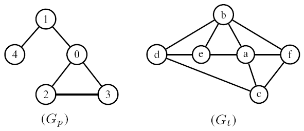
Figure 1: An example for the MCS problem.

Example 1

Figure 1 shows two undirected and unlabelled graphs $G_{p}$ and $G_{t}$, $V_{p}$ = $\{0,1,2,3,4\}$, $V_{t}$ = $\{a,b,c,d,e,f\}$. Initially, $\alpha(v)=\{a,b,c,d,e,f\}$ for each vertex $v$ of $G_{p}$, represented using the pair $\{\langle(0,1,2,3,4),(a,b,c,d,e,f)\rangle\}$.

Then, vertex 0 is chosen in line 11 for branching. The first match added into $curSol$ is $(0,a)$. Consequently, $(1,2,3,4)$ is split into $(1,2,3)$ and $(4)$, and $(b,c,d,e,f)$ is split into $(b,c,e,f)$ and $(d)$, because vertices $1$, $2$ and $3$ are adjacent to the matched vertex $0$, while vertex $4$ is not; and vertices $b$, $c$, $e$ and $f$ are adjacent to the matched vertex $a$, while vertex $d$ is not. The updated $\alpha$ is then represented by $\{\langle(4),(d)\rangle,\langle(1,2,3),(b,c,e,f)\rangle\}$, saying that $\alpha(4)=\{d\}$ and $\alpha(1)=\alpha(2)=\alpha(3)=\{b,c,e,f\}$.

Note that the splitting of $(0,1,2,3,4)$ and $(a,b,c,d,e,f)$ is equivalent to removing $b$, $c$, $e$ and $f$ from $\alpha(4)$, and $d$ from $\alpha(1)$, $\alpha(2)$ and $\alpha(3)$.

More generally, a pair $\langle V^{\prime}_{p},V^{\prime}_{t}\rangle$ is called a label class in McCreesh et al. (2017), where $V^{\prime}_{p}$ ($V^{\prime}_{t}$) is a subset of $V_{p}$ ($V_{t}$), meaning that $\alpha(v)=V^{\prime}_{t}$ for each $v\in V^{\prime}_{p}$. Let $D$ be the set of label classes. When a new match $(v,w)$ is added into $curSol$, Algorithm 1 splits each label class $\langle V^{\prime}_{p},V^{\prime}_{t}\rangle$ in $D$ into two label classes $\langle V^{\prime}_{1p},V^{\prime}_{1t}\rangle$ and $\langle V^{\prime}_{2p},V^{\prime}_{2t}\rangle$ in lines 14 – 21, so that the vertices in $V^{\prime}_{1p}$ ($V^{\prime}_{1t}$) are all adjacent to $v$ ($w$) and the vertices in $V^{\prime}_{2p}$ ($V^{\prime}_{2t}$) are all non-adjacent to $v$ ($w$). Note that $V^{\prime}_{1p}$ and $V^{\prime}_{2p}$, as well as $V^{\prime}_{1t}$ and $V^{\prime}_{2t}$, are disjoint.

This representation of $\alpha$ enables the following branching heuristic and bound computation in McCreesh et al. (2017).

• Given a label class $\langle V^{\prime}_{p},V^{\prime}_{t}\rangle$, there are $|V^{\prime}_{p}|\times|V^{\prime}_{t}|$ matches to try. So, McCreesh et al. first select a label class such that $\max(|V^{\prime}_{p}|,|V^{\prime}_{t}|)$ is the smallest and then the vertex in $V^{\prime}_{p}$ with the greatest degree in line 11 for branching, which is very similar to choosing a label class $\langle V^{\prime}_{p},V^{\prime}_{t}\rangle$ with the smallest $|V^{\prime}_{p}|\times|V^{\prime}_{t}|$ and then breaking ties using vertex degrees. This heuristic is better than the heuristic used in Ndiaye and Solnon (2011) consisting in selecting a label class with the smallest $|V^{\prime}_{t}|$.

• Let $D$ be the set of label classes at a branching point. A label class $\langle V^{\prime}_{p},V^{\prime}_{t}\rangle$ can offer at most $\min(|V^{\prime}_{p}|,|V^{\prime}_{t}|)$ matches to $curSol$. So, the overestimate$(G_{p},G_{t},\alpha)$ function in McCreesh et al. (2017) computes and returns $\sum_{\langle V^{\prime}_{p},V^{\prime}_{t}\rangle\in D}\min(|V^{\prime}_{p}|,|V^{\prime}_{t}|)$, which is equivalent to the bound given by the soft all-different constraint in Ndiaye and Solnon (2011) but is much simpler to compute.

Nevertheless, the branching heuristic in McCreesh et al. (2017) depends heavily on vertex degrees and may not result in the smallest search tree. In the next section, we will propose a new branching heuristic inspired by reinforcement learning.

4 Learning Rewards for Branching

In reinforcement learning, there is an agent and an uncertain environment. The agent is a learner and decision maker, and has a goal or goals. In order to achieve its goal, the agent interacts with the environment by taking actions and observing the impact of its actions to the environment. Concretely, when the agent takes an action, it receives a reward related to its goal from the environment. It has a value function that transforms the cumulative rewards it received over time to a score of the action, representing a prediction of rewards in the future for this action. So, the agent should take the action with the maximum score among all available actions in each step to achieve its goal. For a comprehensive presentation of reinforcement learning and its applications, see, e.g., Sutton and Barto (2018).

Inspired by reinforcement learning, we regard Algorithm 1 as an agent. It has a goal: reach a search tree leaf as early as possible to reduce as much as possible the search tree size. To achieve this goal, the agent adds successively a match $(v,w)$ into $curSol$. However, it usually has many choices of $(v,w)$ in a step and does not know which choice is better. We then regard each choice $(v,w)$ as an action. Then, our key issue now is how to define the reward function and the value function.

As can be seen in Algorithm 1, the algorithm reaches a leaf when UB $\leq|maxSol|$. So, reducing UB quickly allows to reach a leaf quickly. Therefore, we define the reward $R$ for an action $(v,w)$ to be the decrease of UB after taking this action. Concretely, let $D$ be the set of label classes before taking the action $(v,w)$ and $D^{\prime}$ the set of label classes obtained by splitting the label classes in $D$ according to their adjacency to $v$ and $w$ in lines 14 – 21 of Algorithm 1, $R(v,w)$ can be quickly computed as follows.

$~{}~{}~{}~{}R(v,w)=\sum_{\langle V^{\prime}_{p},V^{\prime}_{t}\rangle\in D}\min(|V^{\prime}_{p}|,|V^{\prime}_{t}|)\ -$
$~{}~{}~{}~{}~{}~{}~{}~{}~{}~{}~{}~{}~{}~{}~{}~{}~{}~{}~{}~{}~{}~{}~{}~{}~{}~{}~{}\sum_{\langle V^{\prime\prime}_{p},V^{\prime\prime}_{t}\rangle\in D^{\prime}}\min(|V^{\prime\prime}_{p}|,|V^{\prime\prime}_{t}|)$

Our value function maintains a score $S_{p}(v)$ ($S_{t}(w)$) for each vertex $v\in V_{p}$ ($w\in V_{t}$), initialized to 0. Each time $R(v,w)$ is computed, $S_{p}(v)$ and $S_{t}(w)$ are updated as follows:

$~{}~{}~{}~{}~{}~{}~{}~{}~{}~{}~{}~{}S_{p}(v)\leftarrow S_{p}(v)+R(v,w)$

$~{}~{}~{}~{}~{}~{}~{}~{}~{}~{}~{}~{}S_{t}(w)\leftarrow S_{t}(w)+R(v,w)$

At each branching point (line 11 of Algorithm 1), our algorithm first selects a label class $\langle V^{\prime}_{p},V^{\prime}_{t}\rangle$ with the smallest $\max(|V^{\prime}_{p}|,|V^{\prime}_{t}|)$, and the vertex $v$ in $V^{\prime}_{p}$ with the greatest score $S_{p}(v)$. Then, for each $w$ in $V^{\prime}_{t}$ in the decreasing order of the score $S_{t}(w)$, the algorithm matches $v$ and $w$, and recursively continues the search after adding the match $(v,w)$ into $curSol$. All ties are broken in favor of the vertex with the maximum degree.

Note that original algorithm presented in McCreesh et al. (2017) and our approach all select the label class $\langle V^{\prime}_{p},V^{\prime}_{t}\rangle$ with the smallest $\max(|V^{\prime}_{p}|,|V^{\prime}_{t}|)$. The difference lies in how to choosing $(v,w)$ from $\langle V^{\prime}_{p},V^{\prime}_{t}\rangle$. In McCreesh et al. (2017), $v$ and $w$ are chosen according to their degree. In our approach, $v$ and $w$ are chosen according to their score. We will show the impact of this difference in MCS solving in the next section.

5 Empirical Evaluation

Experiments were performed on Intel Xeon CPUs E5-2680 v4@2.40 gigaHertz under Linux with 4G memory. The cutoff time is 1800 seconds for each instance. We first present the algorithms and the benchmarks used in the experiments, and then present and analyze the experimental results.

5.1 Solvers and Benchmark

The following algorithms (also called solvers) are used in our experiments.

$\bullet$ McSplit McCreesh et al. (2017): An implementation of Algorithm 1 using the label class representation of the $\alpha$ mapping. It is more than an order of magnitude faster than the previous state of the art for unlabelled and undirected MCS instances. It is also extended for labelled graphs.

$\bullet$ McSplit$\downarrow$ McCreesh et al. (2017): A variant of McSplit using a top-down strategy to call the main McSplit method to search for a solution of cardinality $k=|V_{p}|,k-1,k-2,\ldots$ and backtracks when the bound is strictly less than the required cardinality, and terminates when a solution of the required cardinality is found. This strategy is similar to the $k$$\downarrow$ algorithm Hoffmann et al. (2017). McSplit$\downarrow$ is specially designed for the large subgraph isomorphism instances for which McSplit is beaten by $k$$\downarrow$.

$\bullet$ McSplit+RL: An implementation of Algorithm 1 on top of McSplit with reinforcement learning presented in this paper. In other words, the only difference between McSplit+RL and McSplit is the use of reinforcement learning in the branching heuristic in McSplit+RL as presented in Section 4.

$\bullet$ McSplit+RL$\downarrow$: A variant of McSplit+RL using the top-down strategy of McSplit$\downarrow$.

The benchmark consists of two sets of instances.

$\bullet$ Biochemical reactions instances describing the biochemical reaction networks from the biomodels.net . All the 136 graphs are directed, unlabelled bipartite graphs having 9 to 386 vertices. Every pair of graphs gives an MCS instance, resulting in 9316 Bio instances (including 136 self-match pairs).

$\bullet$ Large subgraph isomorphism and MCS instances Hoffmann et al. (2017); McCreesh et al. (2017). This benchmark set includes real-world graphs and graphs generated using random models, such as segmented images, modelling 3D objects, scale-free networks ³. Pattern graphs range from 4 vertices to 900; target graphs range from 10 vertices to 6,671. There are totally 12,427 instances, including: 6278 images instances from images-CVIU11 (there are 43 pattern graphs and 146 target graphs, each pair of pattern graph and target graph resulting in an instance); 1225 LV instances given by each pair of graphs (including two same graphs) among the 49 graphs selected in McCreesh et al. (2017) from the LV set; 3430 largerLV instances from the above 49 LV graphs as pattern and the remaining 70 graphs as target in the LV set; 200 Mesh, 24 PR15, 100 Scalefree and 1170 Si instances used in McCreesh et al. (2017) to evaluate McSplit.

5.2 Performance of the new approach

Table 1 compares the performance of different algorithms for various instance sets. The first column gives the instance set name and the number of instances. The other columns gives the number of instances solved within the 1800s by the corresponding algorithm and the average runtime (inside parentheses) to solve these solved instances. McSplit+RL and McSplit+RL$\downarrow$ solve 130 and 117 instances more than McSplit and McSplit$\downarrow$, respectively. Note that the four solvers share the same implementation, and the only difference between McSplit and McSplit+RL, as well as between McSplit$\downarrow$ and McSplit+RL$\downarrow$, is their branching heuristic.

Table 1: Comparison of the number of instances solved and the average running time (inside parentheses, in seconds) for large MCS instances.

Instance set($\#inst$)	McSplit	McSplit+RL	McSplit$\downarrow$	McSplit+RL$\downarrow$
Bio(9316)	6655(45.8)	6729(40.7)	6818(43.2)	6884(38.8)
Images(6278)	1245(87.1)	1280(87.9)	1266(86.0)	1283(95.6)
LV(1225)	400(59.4)	418(64.8)	410(44.4)	425(39.1)
LargerLV(3430)	578(77.0)	584(119.8)	633(103.7)	650(102.2)
Mesh(200)	–	–	1(57.4)	1(754.8)
PR15(24)	24(12.9)	24(13.5)	24(0.1)	24(0.1)
Scalefree(100)	13(0.0)	13(0.0)	80(7.3)	80(9.0)
Si(1170)	419(22.6)	416(19.8)	1157(3.7)	1159(5.2)
total(21,743)	9,334	9,464	10,389	10,506

As Figure  3 showed, if we exclude the instances that are solved by both McSplit and McSplit+RL within 1s (5s, 10s), McSplit+RL solves 4.27$\%$ (6.26$\%$, 7.54$\%$) more instances than McSplit. The harder the instances are, the greater the effectiveness of reinforcement learning is.

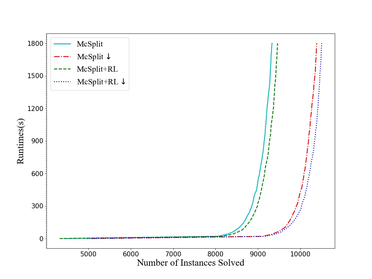
Figure 2: Cactus plot of four solvers showing the number
of instances solved over time among 21,743 instances

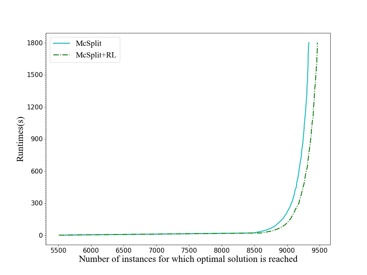
Figure 3: Cactus plot of McSplit and McSplit+RL showing the
number of instances for which the optimal solution is
reached over time among 21,743 instances

Recall that McSplit and McSplit$\downarrow$ are already highly efficient. The results show the effectiveness of the learning approach in designing branching heuristic in a BnB algorithm for the MCS, and the compatibility of the new branching heuristic with the top-down strategy of McSplit$\downarrow$.

5.3 Analysis

The search of a BnB algorithm might be divided into two phases. In phase 1, the algorithm finds an optimal solution $s$; and in phase 2, it proves the optimality of $s$ by proving no better solution exists. Table 2 shows, for a set of representative instances, the total solving time (phase 1 + phase 2) and the time for finding the optimal solution (phase 1) of McSplit and McSplit+RL, respectively. McSplit+RL usually finds the optimal solution more quickly than McSplit, allowing to prune the search more easily in line 8 of Algorithm 1. Note that when the time for finding the optimal solution is smaller, the time for solving an MCS instance usually is also smaller. As Figure  4 showed, McSplit+RL needs less time for finding the optimal solutions of 184 instances than McSplit.

Table 2: Comparison of the solving times ($time$), the runtimes for finding the optimum ($time_{opt}$) and the standard deviation of the number of times selected for branching (in $10^{5}$) of vertex $v$ ($v_{sd}$) and $w$ ($w_{sd}$). $|V_{p}|$ ($|V_{t}|$) denotes the numbers of vertices of pattern (target) graphs. All times are in seconds. The best results are in bold.

InstanceSet-$G_{p}$-$G_{t}$	$|V_{p}|$	$|V_{t}|$	McSplit			McSplit+RL
			$time$	$time_{opt}$	$v_{sd}$ ($w_{sd}$)	$time$	$time_{opt}$	$v_{sd}$ ($w_{sd}$)
Bio-030.txt-061.txt	50	73	372.30	371.60	623.74(204.04)	184.65	183.30	187.68(50.20)
Bio-022.txt-046.txt	38	31	238.65	32.42	309.68(79.55)	1119.95	247.70	1227.46(458.42)
Bio-001.txt-018.txt	46	79	1452.47	0.29	5214.98(545.06)	905.52	0.09	1720.57(214.56)
Images-pattern11-target10	15	3506	0.15	0.07	0.02(0.00)	0.24	0.17	0.02(0.00)
Images-pattern43-target113	89	2877	513.94	513.92	83.54(0.19)	171.95	171.94	16.49(0.07)
Images-pattern24-target119	21	5376	17.51	15.48	2.81(0.00)	9.64	7.20	0.95(0.00)
Images-pattern29-target120	22	4301	9.05	7.88	1.28(0.00)	8.15	7.52	0.61(0.00)
LV-g10-g18	41	64	1103.46	854.83	1002.25(1.28)	1066.48	898.92	1419.91(1.78)
LV-g12-g19	48	64	296.51	296.43	953.03(180.30)	18.60	7.85	13.22(5.98)
LV-g11-g21	42	64	2.06	0.00	4.10(1.00)	3.11	0.00	3.26(0.99)
LV-g10-g17	41	64	203.83	158.45	241.36(20.52)	149.38	131.21	271.18(5.43)
LargerLV-g11-g78	42	627	6.23	6.23	2.33(0.27)	2.13	2.13	0.43(0.07)
LargerLV-g12-g55	48	256	1471.98	1423.98	3580.15(73.53)	562.62	246.93	345.12(30.99)
LargerLV-g13-g70	49	501	213.09	213.08	234.17(0.61)	401.03	197.28	187.58(1.66)
LargerLV-g6-g72	19	561	18.46	18.46	33.90(0.09)	0.02	0.02	0.02(0.00)
LargerLV-g6-g71	19	501	0.01	0.01	0.02(0.00)	0.14	0.02	0.14(0.00)
PR15-pattern1-target	83	4838	9.74	9.68	0.27(0.02)	23.31	23.25	0.54(0.02)
PR15-pattern9-target	68	4838	5.56	5.49	0.24(0.00)	5.09	4.99	0.16(0.00)
Si-si2_b03m_m200.05	40	200	2.08	2.08	3.19(0.94)	0.09	0.09	0.16(0.03)
Si-si2_m4Dr2_m256.02	51	256	1516.22	1516.22	1169.12(127.65)	1156.89	1156.89	460.27(70.89)

Let $b_{p}(v)$ ($b_{t}(w)$) denote the number of times a vertex $v$ in the pattern graph $G_{p}$ ($w$ in the target graph $G_{t}$) is used for branching at line 11 (line 12) of Algorithm 1. Table 2 also gives the standard deviation $v_{sd}$ ($w_{sd}$) of $b_{p}(v)$ ($b_{t}(w)$) when McSplit and McSplit+RL solves these representative graphs. This standard deviation with McSplit+RL is usually significantly smaller than with McSplit, meaning that more vertices participate in branching in McSplit+RL than in McSplit.

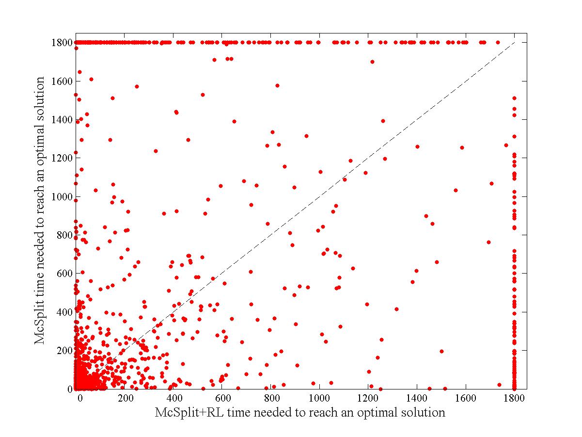
Figure 4: Scatter plot comparing McSplit and McSplit+RL on the time needed to reach an optimal solution for 21,743 instances by excluding the easy instances solved by both McSplit and McSplit+RL within 10s and the too hard instances that none of McSplit and McSplit+RL solves within 1800s. There are 999 points above the diagonal line and 815 points under the diagonal line.

This phenomenon might be explained as follows. McSplit always branches on the vertex with the maximum degree given a label class, concentrating the branching on a small subset of vertices with high degree. However, McSplit+RL can also branch on vertices with lower degree in a label class, because reinforcement learning discovers that these vertices allow a big bound decrease.

In summary, the search of McSplit+RL is more diversified while leading to quick pruning, explaining why McSplit+RL usually finds the optimal solution more quickly than McSplit.

6 Conclusion

We proposed a branching heuristic inspired from reinforcement learning in a BnB algorithm for the MCS, by regarding the algorithm as an agent and a match $(v,w)$ as an action. The reward of an action is the decrease of the upper bound and the score of a vertex is the sum of rewards of the actions it participated in the past. Then, the algorithm uses these scores to select the action $(v,w)$ for branching. Intensive experiments show that this branching heuristic allows to solve significantly more instances, because it allows a more diversified search.

Our results suggest that reinforcement learning is a very promising tool for NP-hard problem solving. We will improve the reward and value function definitions to further improve our branching heuristic for the MCS in the future.

References

- Bahiense et al. [2012] Laura Bahiense, Gordana Manic, Breno Piva, and Cid C. de Souza. The maximum common edge subgraph problem: A polyhedral investigation. Discrete Applied Mathematics, 160(18):2523–2541, 2012.
- Bunke and Messmer [1995] Horst Bunke and Bruno T. Messmer. Efficient attributed graph matching and its application to image analysis. In Image Analysis and Processing, 8th International Conference, ICIAP, volume 974 of LNCS, pages 45–55. Springer, 1995.
- Cao et al. [2011] Ning Cao, Zhenyu Yang, Cong Wang, Kui Ren, and Wenjing Lou. Privacy-preserving query over encrypted graph-structured data in cloud computing. In 2011 International Conference on Distributed Computing Systems, ICDCS, pages 393–402. IEEE Computer Society, 2011.
- Conte et al. [2004] Donatello Conte, Pasquale Foggia, Carlo Sansone, and Mario Vento. Thirty years of graph matching in pattern recognition. International Journal of Pattern Recognition and Artificial Intelligence, 18(3):265–298, 2004.
- Cootes et al. [2007] Adrian P. Cootes, Stephen H. Muggleton, and Michael J.E. Sternberg. The identification of similarities between biological vetworks: application to the metabolome and interactome. Molecular Biology, 369(4):1126–1139, 2007.
- Cordella et al. [2004] Luigi P. Cordella, Pasquale Foggia, Carlo Sansone, and Mario Vento. A (sub)graph isomorphism algorithm for matching large graphs. IEEE Trans. Pattern Anal. Mach. Intell., 26(10):1367–1372, 2004.
- Faccioli et al. [2005] P. Faccioli, P. Provero, C. Herrmann, A. M. Stanca, C. Morcia, and V.Terzi. From single genes to co-expression networks:extracting knowledge from barleyfunctional genomics. Plant Molecular Biology, 58(5):739–750, 2005.
- Giugno et al. [2013] Rosalba Giugno, Vincenzo Bonnici, Nicola Bombieri, Alfredo Pulvirenti, Alfredo Ferro, and Dennis Shasha. Grapes: a software for parallel searching on biological graphs targeting multi-core architectures. PLOS ONE, 8(10):e76911, 2013.
- Hoffmann et al. [2017] Ruth Hoffmann, Ciaran McCreesh, and Craig Reilly. Between subgraph isomorphism and maximum common subgraph. In AAAI, pages 3907–3914. AAAI Press, 2017.
- Levi [1973] G. Levi. A note on the derivation of maximal common subgraphs of two directed or undirected graphs. Calcolo, 9(4):341–352, 1973.
- Liu and Lee [2001] Jianzhuang Liu and Yong Tsui Lee. A graph-based method for face identification from a single 2d line drawing. IEEE Trans. Pattern Anal. Mach. Intell., 23(10):1106–1119, 2001.
- McCreesh et al. [2016] Ciaran McCreesh, Samba Ndojh Ndiaye, Patrick Prosser, and Christine Solnon. Clique and constraint models for maximum common (connected) subgraph problems. In CP, volume 9892 of Lecture Notes in Computer Science, pages 350–368. Springer, 2016.
- McCreesh et al. [2017] Ciaran McCreesh, Patrick Prosser, and James Trimble. A partitioning algorithm for maximum common subgraph problems. In IJCAI, pages 712–719. ijcai.org, 2017.
- McGregor [1982] James J. McGregor. Backtrack search algorithms and the maximal common subgraph problem. Softw., Pract. Exper., 12(1):23–34, 1982.
- Ndiaye and Solnon [2011] Samba Ndojh Ndiaye and Christine Solnon. CP models for maximum common subgraph problems. In CP, volume 6876 of Lecture Notes in Computer Science, pages 637–644. Springer, 2011.
- Solnon et al. [2015] Christine Solnon, Guillaume Damiand, Colin de la Higuera, and Jean-Christophe Janodet. On the complexity of submap isomorphism and maximum common submap problems. Pattern Recognition, 48(2):302–316, 2015.
- Solnon [2010] Christine Solnon. Alldifferent-based filtering for subgraph isomorphism. Artif. Intell., 174(12-13):850–864, 2010.
-
Sutton and
Barto [2018]
Richard S. Sutton and Andrew G. Barto.
Reinforcement Learning: An introduction (2nd Ed.).
2018.
http://www.incompleteideas.net/
book/the-book-2nd.html. - Vismara and Valery [2008] Philippe Vismara and Benoît Valery. Finding maximum common connected subgraphs using clique detection or constraint satisfaction algorithms. volume 14 of Communications in Computer and Information Science, pages 358–368. Springer, 2008.