Planted Hitting Set Recovery in Hypergraphs
Abstract.
In various application areas, networked data is collected by measuring interactions involving some specific set of core nodes. This results in a network dataset containing the core nodes along with a potentially much larger set of fringe nodes that all have at least one interaction with a core node. In many settings, this type of data arises for structures that are richer than graphs, because they involve the interactions of larger sets; for example, the core nodes might be a set of individuals under surveillance, where we observe the attendees of meetings involving at least one of the core individuals. We model such scenarios using hypergraphs, and we study the problem of core recovery: if we observe the hypergraph but not the labels of core and fringe nodes, can we recover the “planted” set of core nodes in the hypergraph?
We provide a theoretical framework for analyzing the recovery of such a set of core nodes and use our theory to develop a practical and scalable algorithm for core recovery. The crux of our analysis and algorithm is that the core nodes are a hitting set of the hypergraph, meaning that every hyperedge has at least one node in the set of core nodes. We demonstrate the efficacy of our algorithm on a number of real-world datasets, outperforming competitive baselines derived from network centrality and core-periphery measures.
1. Introduction
The data we can collect in practice is typically incomplete in several fundamental and recurring ways, and this is particularly true for graph and network data modeling complex systems throughout the social and biological sciences (Laumann et al., 1989; Kuny, 1997; Kossinets, 2006; Gile and Handcock, 2010; Guimerà and Sales-Pardo, 2009). One common type of incompleteness arises from a particular type of data collection procedure where one wants to record all interactions involving a set of core nodes . This results in what is sometimes called a “core-fringe” structure (Benson and Kleinberg, 2018b), where the resulting network structure contains the core nodes along with a (potentially) much larger set of fringe nodes that are observed in some interaction with a node in . For example, in survey data, might represent a set of respondents, and a set of individuals with whom they interact; this is a common result in snowball and respondent-driven sampling (Heckathorn, 2011; Gile and Handcock, 2010; Goel and Salganik, 2010). Another scenario arises in restrictions on surveillance. For example, the Enron (Klimt and Yang, 2004) and Avocado111https://catalog.ldc.upenn.edu/LDC2015T03 email datasets are common data sources for email and network research; both datasets have a core comprised of employees of a company and a fringe of people outside the company that come from emails sent from or received by members of .
One can imagine similar scenarios in a variety of settings. In intelligence data, one might record all of the attendees at meetings that involve at least one of a set of individuals under surveillance. In a similar manner, telecommunications providers can observe group text messages where only some of the members of the group are subscribers. Furthermore, measurements of Internet structure from service providers at the IP-layer from individual service providers provide only a partial measurement (Tsiatas et al., 2013), and large-scale Web crawls do not encapsulate the entire network structure of hyperlinks (Boldi et al., 2004, 2014).
While a dataset may be equipped with labels of which nodes are members of the core and which are members of the fringe, there are several situations in which such labels are unavailable. For example, consider the email datasets described above. Such data could be released by a hacker from outside the organization, or a leaker from inside it, who has collected email from a set of core accounts but not released the identity of the accounts (Hier and Greenberg, 2009). Similarly, in the case of intelligence data that records attendees of meetings, the data could be released with the identities of the individuals under surveillance redacted. In other cases, the metadata may be lost simply to issues of data maintenance, and such concerns are central to the research areas of data provenance and preservation (Buneman et al., 2001; Lynch, 2008; Simmhan et al., 2005; Tan, 2004).
The question of recovering the identity of the core nodes in a dataset with core-fringe structure is therefore a fundamental question arising in different applications, and for multiple different reasons.
Core-Fringe Recovery in Hypergraphs. Here, we study the problem of identifying the set of core nodes, when the labels of which nodes are core and which are fringe are unavailable and the data is represented by a hypergraph—that is, a set of nodes along with a set of hyperedges that each connect multiple nodes. Figure 1 illustrates this model. The hypergraph model is apt for many of the scenarios described above, including emails, meeting attendees, and group messages. While the hypergraph model is richer than a more standard graph model, the higher-order structure also presents challenges. If a hyperedge connects a (latent) core node and several fringe nodes, a core recovery algorithm will have to consider all nodes in the hyperedge as possible candidates for the core.
We first provide theoretical results that motivate the development of an algorithm for recovery of the core. The key structural property of our analysis is that the core nodes constitute a hitting set, meaning every hyperedge in the hypergraph has at least one node in the core (Fig. 1). This property comes from how the data is measured—every included hyperedge comes from an interaction of a member of the core with some other set of nodes. We thus think of the core as a “planted” hitting set that we must find in the data. Our first theoretical results rely on two assumptions (both relaxable, to some extent): the planted hitting set corresponding to the core is (i) minimal, that is, no node could be removed to make the hitting set smaller; and (ii) relatively small, i.e., bounded by a constant . We analyze how large the union of all minimal hitting sets, denoted , can be. We build upon results in fixed-parameter tractability (Damaschke, 2006; Damaschke and Molokov, 2009) to show that is in the worst case, where is the size of the largest hyperedge; importantly, this bound is independent of the hypergraph’s size, and is guaranteed to contain our planted hitting set if it meets the modeling assumptions.
Furthermore, we prove that a classical greedy approximation algorithm for set cover relates to partial recovery of the planted hitting set. In a hypergraph where is the size of the largest hyperedge, we show that the output of the algorithm must overlap with the planted hitting set by at least a fraction of the nodes, provided that the hitting set size is within a constant factor of the minimum hitting set size.
Combining these two main results leads to our algorithm, which we call the union of minimal hitting sets (UMHS). This algorithm is practical and scalable, using only simple subroutines and having computational complexity roughly linear in the size of the data. The idea is to run the greedy algorithm multiple times with random initialization to find several minimal hitting sets and then to simply take the union of these hitting sets. The first part of our theory says that the output should not grow too large, and the second part of our theory says the output should also overlap the planted hitting set. We show that our method consistently outperforms a number of baselines derived from network centrality and core-periphery structure for hypergraphs on several real-world datasets.
Our approach to the planted hitting set problem is purely combinatorial. This contrasts with typical planted problems such as the stochastic block model and planted clique recovery, which are based on probabilistic structure. Thus, the methods we use are fundamentally different than what is common for these types of problems. Moreover, we show that if random block-model-type structure exists for our problem, then the problem becomes substantially easier.
2. Problem setup and theoretical results for core recovery
We start with some formal definitions to facilitate our presentation of the theoretical results. A hypergraph consists of a set of nodes and a set of hyperedges , each a subset of of size at least two. The rank of a hypergraph is the maximum size of any hyperedge, i.e., . A hypergraph is called -uniform if all hyperedges have cardinality equal to .
In our setup, there is some unidentified subset that is designated as the set of “core nodes.” Our goal is to find , knowing that is a hitting set of (i.e., for every , there is some ). We say that is planted since we do not know its identity. Absent any additional information, we are helpless—it could be that . However, we can do better by assuming two properties of (both relaxable): (i) is a minimal hitting set in and (ii) . Under these constraints, it is certainly true that is contained in the union of all minimal hitting sets, which is a principle object of our analysis:
Definition 1.
Given a hypergraph , is the union of all minimal hitting sets of of size at most .
We next show bounds on that are independent of the size of the graph. This says that is contained in a relatively small set if it satisfies the conditions. Furthermore, we can find in time exponential in but polynomial in the size of the graph; however, we develop more practical algorithms in Section 3. After, we relax the assumptions on minimality and get results on partial recovery, i.e., algorithms that are guaranteed to find a part of . Finally, we show how these results improve under a random hypergraph model.
2.1. Minimal hitting sets
First let us suppose that we are given and asked to find , where we know that is minimal and . We ask the following question: is it possible to find a small set , whose size is independent of , such that ? In this section, we answer the question in the affirmative.
We at least know that the union of all minimal hitting sets of size at most , (Definition 1), must contain . But how large can this set be? The following result says that actually can’t be that large.
Lemma 2 ((Damaschke and Molokov, 2009; Damaschke, 2006)).
In a hypergraph of rank , has size in the worst case.
Damaschke and Molokov established the upper bound using sophisticated techniques from parameterized complexity theory (Damaschke and Molokov, 2009). Here, we prove the same upper bound with a simpler, self-contained proof that uses the celebrated sunflower lemma of Erdös and Rado (Erdös and Rado, 1960). The lower bound was stated by Damashke (Damaschke, 2006) with a brief proof sketch. We provide a full proof for completeness. A consequence of these results is the following:
Theorem 3.
Let be a planted minimal hitting set with in a hypergraph of rank . Then we can find a set of size that is guaranteed to contain .
We begin by providing the self-contained proof of the upper bound in Theorem 3. Namely, let be a hypergraph of rank , and let be the union of all minimal hitting sets in of size at most . We will find a function so that . To find such a function, we use a combinatorial structure called a sunflower (Bollobás, 1986). A collection of sets is an -sunflower if for all pairs of distinct sets , , the pairwise intersection is equal to the mutual intersection . The term comes from the fact that we can think of the as the “petals” of the sunflower: they share a “center” and are otherwise pairwise disjoint from each other. A famous theorem of Erdös and Rado asserts that every sufficiently large collection of sets must contain a large sunflower.
Lemma 4 (Sunflower Lemma (Erdös and Rado, 1960)).
Define the function . Any collection of more than sets, each of size at most , must contain a -sunflower.
We use this result to find the desired function . Subsequently, we establish an asymptotically matching lower bound.
Lemma 5.
Let be a hypergraph of rank . Then .
Proof.
We assume that has at least one hitting set of size at most , as otherwise the statement of Lemma 5 holds with equal to the empty set. We modify according to the following iterative procedure, which operates in discrete phases. We start by defining , and produce a succession of hypergraphs , with the hypergraph at the end of phase . For each hypergraph , let denote the set of all hitting sets of size at most in , and let denote the set of all minimal hitting sets of size at most in . We will establish by induction that each hypergraph has at least one hitting set of size at most .
At the start of phase , we ask whether has more than hyperedges, where is the function from Lemma 4. If it doesn’t, we declare the procedure to be over. If it does, then we find a -sunflower in the set of hyperedges, consisting of hyperedges .
Now, the core of the sunflower found in phase , which we will denote by must be non-empty, for if it were empty, then would contain pairwise disjoint hyperedges, and hence could not have a hitting of size at most . We define as follows: starting from , we remove the hyperedges and add the hyperedge . We observe the following properties.
-
(1)
Every hitting set in of size at most must intersect .
-
(2)
, and hence .
To see Property (1), By the definition of a sunflower, the sets are pairwise disjoint for . Thus, if is a set of size at most that doesn’t contain any nodes of , then it must be disjoint from at least one of the sets , and hence it can’t be a hitting set for . The definition of is as follows: starting from , we remove the hyperedges and add the hyperedge . Since and are hypergraphs on the same node sets, their respective collections of hitting sets and are also over the same sets of elements.
Now, let . Then by Property (1), it must intersect . Since is the only hyperedge in but not , it follows that is a hitting set for , and hence . Conversely, let . Since for , it must be that intersects each . Since are the only hyperedges in but not , it follows that . Thus, , and so they are equal as sets.
We apply the same process in each phase, producing from , then producing from and so forth. By induction using Property (2), since contains at least one hitting set of size at most , so does , as required. Since the procedure reduces the number of hyperedges in each phase, it must eventually terminate, in some phase . We write and by applying Property (2) transitively,
| (1) |
We say that a node is isolated if it does not belong to any hyperedge. Let be the set of non-isolated nodes of . Since the procedure stopped when faced with , had at most hyperedges. Since each hyperedge has most elements, we have
| (2) |
and hence is bounded by . Finally, recall that is the union of all minimal hitting sets in of size at most . We can write , and by Eq. 1, . No minimal hitting set in can contain an isolated node , since then would also be a hitting set in . From this, , and by Eq. 2. ∎
We now show asymptotic tightness for constant , by constructing a family of hypergraphs for which . The following lemma combined with Lemma 5 proves Theorem 3.
Lemma 6.
For each constant , there exists an infinite family of rank- hypergraphs and parameters , with both the number of nodes in and going to infinity, for which .
Proof.
Here we present the full proof of Lemma 6. This lemma was stated without a complete proof by Damaschke (Damaschke, 2006, Proposition 9).
For a parameter , consider a graph that consists of disjoint complete -ary trees of depth . We will refer to the roots of the trees in as the root nodes of , and to the leaves of the trees in as leaf nodes. Let be the hypergraph on the node set of whose hyperedges consist of all root-to-leaf paths in , from the root of one of the trees in to a leaf of the corresponding tree (the example of for is in Fig. 2). All edges in have size . Let be any function that maps nodes of to numbers in with the following properties: (i) is a bijection from the roots of to ; and (ii) for each non-leaf node in , is a bijection from the children of to . For each node , we will call its label (with respect to ), and we will say that is a consistent labeling if it satisfies (i) and (ii). Let be unique leaf node for which all the nodes on the root-to-leaf path have the label .
For a consistent labeling , let be the set of all nodes satisfying two properties: (i) for all nodes on the unique path from a root of to (other than itself), and (ii) . Let . We observe the following two facts.
-
(1)
For every consistent labeling , the set is a minimal hitting set for .
-
(2)
Every node v of belongs to at least one set of the form for some consistent labeling .
To prove (1), we claim that is a hitting set. Consider any hyperedge of , consisting of a root-to-leaf path in . If all nodes on have label , then the leaf node of is , and hence intersects . Otherwise, consider the first node on the path that has a label unequal to . Thus, , and again intersects and is a hitting set. We now argue that it is minimal. If we delete from , then would be disjoint from the hyperedge consisting of the root-to-leaf path to . If we delete some other , then a hyperedge that passes through does not pass through any other node of on its way from root to leaf, and so would be disjoint from .
To prove (2), we simply choose any consistent labeling such that for all nodes on the unique path from a root of to (other than itself), and .
Now, we consider the size of a set of the form . Since contains nodes from each of the first levels of the trees in , and from the lowest level, we have
We define . Since each set is a minimal hitting set of size , from (2) we see that the union of all minimal hitting sets of size is the entire node set of .
The number of nodes in is greater than , and hence . Since , we have that . ∎
2.2. Non-minimal hitting sets
Here we present results on which types of nodes in a planted hitting set must be contained in when the hitting set is itself not minimal. This matters in practice, when may not be minimal.
Classes of nodes that must be in . Our first result is that a node in must appear in if all the other nodes in a hyperedge containing are not in .
Lemma 7.
Let be a rank- hypergraph with planted hitting setting . If and there exists a hyperedge with with , then .
Proof.
We perform a pruning of as follows. Check whether there exists a node with still being a hitting set of smaller cardinality. If this is the case, update to and continue pruning. Upon termination, the remaining set is a minimal hitting set . Clearly, so that . However, since is a hyperedge where . ∎
The above lemma provides a class of nodes in a planted hitting set which are guaranteed to be in the union of minimal hitting sets of size no more than that of the planted hitting set itself. Next, we show that nodes adjacent to other nodes deeply integrated into must also be in . Formally, define a node to be in the interior of a hitting set if all hyperedges containing are comprised entirely of nodes in . Our next result is that a node in must appear in if all the other nodes in a hyperedge containing are in the interior of .
Lemma 8.
Let be a rank- hypergraph with planted hitting set . If and there exists a hyperedge where are in the interior of , then .
Proof.
Since are in the interior of , is a hitting set as well. Now perform pruning on as in the previous proof, the output of which is , and since clearly , we must have that . Clearly was not deleted during pruning since is a hyperedge with , so that . ∎
Greedy matchings intersect the planted hitting set. One way of finding hitting sets is through greedy algorithms for set cover. The classical matching algorithm is simple (Algorithm 1): loop through each hyperedge and if no vertex in the current hyperedge is in the current cover , add all to the . The greedy algorithm produces a set that is both a hitting set and a maximal matching. To see that it is a hitting set, suppose that all nodes in a hyperedge were not added. Then would have been added to at the time the algorithm processed it. The output is a maximal matching because if we could append another hyperedge to , then would have already been added to when the algorithm processed it.
Let be the minimum hitting set size (the smallest size of all minimal hitting sets). The output of Algorithm 1 is an -approximation if the hypergraph is an -uniform hypergraph: in the worst case, any hitting set contains at least one of nodes from each hyperedge, and we therefore have . It turns out that this greedy algorithm must also partially overlap with the planted hitting set. We formalize this in the following lemma.
Lemma 9.
Let for some hitting set . If the input to Algorithm 1 is an rank- hypergraph, then the output satisfies .
Proof.
Let be the number of vertices in the hyperedge containing the least vertices. The set contains within itself all vertices from hyperedges where satisfies . Since is a hitting set, it must contain at least one vertex from each of the hyperedges in . From this, we obtain . ∎
Lemma 9 guarantees that the greedy algorithm will output a result that overlaps any hitting set, including the planted one. Thus, we immediately get the following corollary.
Corollary 10.
If the planted hitting set has size then the output of Algorithm 1 is a set with , i.e., intersects at least a fraction of of .
We can process the hyperedges in any order within Algorithm 1, and this will be important for our practical recovery algorithm that we develop later. Another immediate corollary of Lemma 9 says that regardless of the processing, the outputs must be fairly similar.
Corollary 11.
Any two outputs and of Algorithm 1 satisfy .
Thus far, we have made no assumptions on the structure of the hypergraph. In the next section, we show that assuming a stochastic block model type hypergraph structure gives substantial improvements in recovery.
2.3. Recovery in a random hypergraph model
Imposing structure on and will enable us to obtain more information. In particular, we will show how we can obtain tighter bounds under certain random graph models for 3-uniform hypergraphs. Let us assume that the hyperedges are generated according to a stochastic block model (SBM) for hypergraphs (Ghoshdastidar and Dukkipati, 2014). One block will be the core and the other the fringe nodes . We assume that there is zero probability of a hyperedge containing only nodes in . Explicitly, we will state that the probability of a hyperedge between nodes in is while the probability of a hyperedge containing at least one node in and at least one node in is .
We first provide a lemma on the independence number of hypergraphs drawn from the hypergraph SBM. This will help us control the size of .
Lemma 12.
Let be the independence number of an -uniform hypergraph drawn from the SBM on vertices. Then
Proof.
We follow a proof technique common in the combinatorics literature (Kostochka et al., 2014). Let , the size- subsets of vertices of , and an indicator random variable for being an independent set of , so only happens when all possible hyperedges among the vertices of do not appear in the hyperedge set of . Note that this happens with probability . Thus,
so that , as desired. ∎
This lemma enables a result for 3-uniform hypergraphs.
Theorem 13.
Proof.
Theorem 13 enables us to find a small set that contains the core with high probability.
Theorem 14.
Let with be a planted hitting set in a 3-uniform hypergraph drawn from the SBM parameterized by and with nodes for some . Then with high probability in , there is a set with and .
Proof.
The number of ways to link a vertex in the core to two nodes outside the core is so that the probability of a node having at least one hyperedge to two nodes outside the core is . Thus is the probability of each of the nodes in the core having at least one hyperedge to two nodes outside the core. This probability tends to 1 as , so by using Lemma 7, with probability tending to 1. Setting and using Theorem 13 gives the result. ∎
Of course, the above theorem is only useful if we have a bound on the quantity since only in that case are we able to improve our bound on the size of from to . Absent any additional information, (Damaschke and Molokov, 2009).
In the following section, we build a practical algorithm for recovery of planted hitting sets based on the union of minimal hitting sets, the theory for which was examined in this section.
3. A practical recovery algorithm
Based on the theoretical results described above, we now develop a practical algorithm for recovering a planted hitting set in a hypergraph. To put our theory into practice, we place several of our theoretical results in context. First, Lemma 9 says that Algorithm 1 produces outputs that must overlap with the planted hitting set. Moreover, this was true regardless of the order in which we processed the edges. Thus, the basic idea of our algorithm is simple: we find many hitting sets from Algorithm 1 and take their union.
By 10, if the planted hitting set is close to a minimum hitting set, then any iteration of Algorithm 1 will recover a large fraction of it. Furthermore, by 11, the outputs of Algorithm 1 must overlap by a modest amount, so taking the unions of outputs cannot grow too fast. To limit growth further, we can prune the output of Algorithm 1 to be a minimal hitting set (this also tends to give better results in practice). Now, Theorem 3 says that the union of pruned outputs will be bounded, provided the graph is large enough and that the outputs are small enough. This turns out to be the case in our experimental results. To summarize, our procedure is as follows: (i) Find a hitting set from Algorithm 1, processing the hyperedges in a random order; (ii) Prune to be a minimal hitting set ; and (iii) Repeat steps (i) and (ii) several times and output the union of the found in step (ii). Again, the key result is that Lemma 9 holds regardless of the ordering in which the hyperedges are processed. The algorithm is formalized in Algorithm 2. A similar algorithm for the special case of -uniform hypergraphs (i.e., graphs) was recently analyzed (Benson and Kleinberg, 2018b).
The output of Algorithm 2 is by construction a union of minimal hitting sets (UMHS) of the input hypergraph , and we will refer to the algorithm as UMHS. The theoretical guarantees from Section 2.1 apply here. Specifically, under the assumption that the planted hitting set is itself minimal, we are guaranteed full recovery with sufficient iterations. However, planted hitting sets are rarely minimal in practice (in fact, they are not for the datasets we consider). However, Theorem 3 still guarantees that the output of the algorithm will not grow very quickly.
Importantly, Algorithm 2 runs in time linear in the number of hyperedges. In particular, suppose the input is a hypergraph of rank with a minimum hitting set of size . Then the algorithm produces an output in time. This happens because every call to Algorithm 1 takes time, while pruning to be a minimal hitting set of requires time in the worst case (in practice, it is much faster). Thus, in the worst case, pruning to a minimal hitting set takes more time than one iteration of the greedy algorithm. However, this increase in processing time is not prohibitive since it only increases by the constant factor . Nonetheless, pruning is crucial as in practice we find that it drastically reduces the output size.
4. Experimental results
We now test Algorithm 2 on a number of real-world datasets and compare and find that it consistently outperforms several baselines derived from network centrality and core-periphery structure. We also show that we do not need too many iterations within Algorithm 2 (the parameter ) for our performance levels.
| number of nodes | size of core () | number of hyperedges | ||||||||||
| Enron | 1,283 | 976 | 869 | 84 | 73 | 77 | 2,361 | 1,048 | 614 | |||
| Avocado | 5,521 | 3,510 | 2,965 | 227 | 218 | 211 | 21,690 | 12,455 | 6,973 | |||
| W3C | 1,778 | 749 | 308 | 353 | 237 | 125 | 1,882 | 389 | 88 | |||
| DBLP | 3–875 | 4–514 | 5–261 | 3–114 | 4–90 | 5–55 | 1–753 | 1–265 | 1–78 | |||
| Math tags | 93–1,180 | 97–1,239 | 121–1,153 | 3–15 | 4–15 | 5–15 | 112–13,771 | 128–17,424 | 98–13,410 | |||
| Ubuntu tags | 96–2,005 | 402–2,043 | 225–1,991 | 3–15 | 4–15 | 5–15 | 94–12,990 | 437–13,210 | 220–9,905 | |||
4.1. Data
The six datasets we use broadly fall into three broad classes based on the types of planted hitting problems we derive from them. The first group is three email datasets (Enron, Avocado, and W3C), where the planted hitting set is a group of people at an organization, and hyperedges come from emails involving multiple addresses. Next, in the DBLP dataset, a planted hitting set is a set of authors who publish at the same conference in a given year, and we consider several such conferences. Finally, in the Stack Exchange tagging datasets, the core is a one-hop neighborhood of a node, which is a hitting set for the two-hop neighborhood of the node; again, we consider several hitting sets. In this sense, the DBLP and tagging datasets are collections of hypergraphs with core-fringe structure.
Enron (Klimt and Yang, 2004), Avocado, and W3C (Craswell et al., 2005). The hyperedges in these datasets are emails, where the nodes are the sender and all receivers (more specifically, their email addressses). Repeated hyperedges are discarded. In the Enron data, the core is a set of 150 employees whose email was made public when the company was under United States federal investigation. The Avocado corpus comes from a now-defunct technology company, where the core are employee email accounts (we exclude email accounts associated with conference rooms or mailing lists from the core). Finally, the the W3C dataset comes from emails on mailing lists related to W3C; the core is all email addresses with a w3c.org domain.
DBLP. DBLP is an online computer science bibliography. We construct a hypergraph from coauthorship data in conference proceedings. We randomly sampled 50 conferences with relatively small cores and constructed a set of core nodes from the authors of a given conference in a randomly selected year. We then took the core-fringe hypergraph to be all hyperedges involving at least one of these authors.
Math and Ubuntu tags (Benson et al., 2018). These datasets come from tags applied to questions on the Math and AskUbuntu Stack Exchange web sites. Hyperedges are sets of tags that have been applied to the same question. For both Stack Exchanges, we sampled 50 tags with relatively small cores uniformly at random. We then formed a core set from the one-hop neighborhood of that tag, i.e., from the tag and all tags that appear as co-tags with the tag. The set is then a planted hitting set for the two-hop neighborhood of that tag.
We constructed 3-, 4-, and 5-uniform hypergraphs (derived as sub-hypergraphs) from these datasets to facilitate comparison of UMHS performance to that of other centrality-based algorithms (furthermore, Stack Exchange only has at most 5 tags in one post). Table 1 lists summary statistics of the datasets.
| Dataset | UMHS | Degree | Clique-eigen | Z-eigen | H-eigen | Borgatti-Everett | k-core | ||
|---|---|---|---|---|---|---|---|---|---|
| Precision @ | Enron | 3 | 0.52 | 0.33 | 0.14 | 0.11 | 0.13 | 0.14 | 0.33 |
| 4 | 0.53 | 0.33 | 0.21 | 0.18 | 0.16 | 0.19 | 0.33 | ||
| 5 | 0.49 | 0.25 | 0.16 | 0.14 | 0.17 | 0.14 | 0.17 | ||
| Avocado | 3 | 0.91 | 0.60 | 0.56 | 0.54 | 0.58 | 0.59 | 0.58 | |
| 4 | 0.82 | 0.57 | 0.52 | 0.33 | 0.53 | 0.52 | 0.56 | ||
| 5 | 0.72 | 0.56 | 0.49 | 0.34 | 0.50 | 0.49 | 0.33 | ||
| W3C | 3 | 0.51 | 0.38 | 0.20 | 0.11 | 0.21 | 0.19 | 0.35 | |
| 4 | 0.43 | 0.43 | 0.30 | 0.30 | 0.31 | 0.30 | 0.40 | ||
| 5 | 0.30 | 0.42 | 0.31 | 0.34 | 0.33 | 0.33 | 0.41 | ||
| DBLP | 3 | 0.590.15 | 0.630.15 | 0.440.24 | 0.420.28 | 0.410.26 | 0.410.26 | 0.440.21 | |
| 4 | 0.480.15 | 0.580.17 | 0.400.27 | 0.360.29 | 0.390.28 | 0.380.31 | 0.400.22 | ||
| 5 | 0.390.15 | 0.650.22 | 0.560.31 | 0.590.35 | 0.570.31 | 0.560.31 | 0.560.25 | ||
| Math tags | 3 | 0.800.14 | 0.580.13 | 0.430.15 | 0.410.14 | 0.450.13 | 0.500.14 | 0.430.12 | |
| 4 | 0.710.18 | 0.480.12 | 0.380.12 | 0.310.14 | 0.390.11 | 0.310.10 | 0.380.11 | ||
| 5 | 0.610.19 | 0.400.10 | 0.330.10 | 0.240.11 | 0.320.10 | 0.310.10 | 0.330.10 | ||
| Ubuntu tags | 3 | 0.800.09 | 0.580.16 | 0.360.13 | 0.320.13 | 0.400.15 | 0.550.16 | 0.360.12 | |
| 4 | 0.780.13 | 0.500.16 | 0.380.17 | 0.300.15 | 0.400.17 | 0.330.17 | 0.380.15 | ||
| 5 | 0.690.18 | 0.380.14 | 0.280.12 | 0.230.13 | 0.270.12 | 0.250.12 | 0.280.14 | ||
| Area under PR curve | Enron | 3 | 0.18 | 0.15 | 0.08 | 0.07 | 0.07 | 0.08 | 0.15 |
| 4 | 0.16 | 0.16 | 0.10 | 0.09 | 0.09 | 0.10 | 0.16 | ||
| 5 | 0.17 | 0.13 | 0.10 | 0.10 | 0.10 | 0.10 | 0.10 | ||
| Avocado | 3 | 0.43 | 0.38 | 0.33 | 0.31 | 0.36 | 0.37 | 0.36 | |
| 4 | 0.38 | 0.35 | 0.30 | 0.15 | 0.31 | 0.30 | 0.34 | ||
| 5 | 0.34 | 0.34 | 0.28 | 0.16 | 0.28 | 0.27 | 0.33 | ||
| W3C | 3 | 0.36 | 0.27 | 0.20 | 0.19 | 0.20 | 0.20 | 0.25 | |
| 4 | 0.40 | 0.37 | 0.31 | 0.31 | 0.31 | 0.31 | 0.35 | ||
| 5 | 0.41 | 0.41 | 0.38 | 0.38 | 0.38 | 0.38 | 0.41 | ||
| DBLP | 3 | 0.570.17 | 0.520.18 | 0.390.24 | 0.400.28 | 0.380.25 | 0.370.25 | 0.470.23 | |
| 4 | 0.470.19 | 0.460.17 | 0.360.26 | 0.350.27 | 0.360.26 | 0.360.29 | 0.390.22 | ||
| 5 | 0.540.23 | 0.570.24 | 0.530.31 | 0.580.34 | 0.540.31 | 0.540.31 | 0.580.26 | ||
| Math tags | 3 | 0.680.18 | 0.360.14 | 0.210.13 | 0.190.12 | 0.230.12 | 0.270.14 | 0.260.12 | |
| 4 | 0.560.20 | 0.250.11 | 0.170.11 | 0.120.11 | 0.170.09 | 0.110.07 | 0.170.10 | ||
| 5 | 0.480.21 | 0.180.08 | 0.130.07 | 0.080.07 | 0.120.06 | 0.110.06 | 0.140.07 | ||
| Ubuntu tags | 3 | 0.650.14 | 0.370.17 | 0.150.11 | 0.130.11 | 0.190.13 | 0.330.17 | 0.200.12 | |
| 4 | 0.640.16 | 0.280.16 | 0.180.14 | 0.120.12 | 0.190.15 | 0.140.14 | 0.180.13 | ||
| 5 | 0.540.18 | 0.170.11 | 0.100.08 | 0.070.09 | 0.090.08 | 0.080.08 | 0.120.10 |
4.2. Recovery results
We tested the UMHS algorithm on several datasets, and it outperforms other algorithms consistently. For baselines, we use two techniques. First, we use notions of network centrality developed for hypergraphs with the idea that nodes in the core could be identified via large centrality scores. Specifically, we compare against (i) hypergraph degree centrality (the number of hyperedges in which a node appears) (Kapoor et al., 2013); (ii) clique graph eigenvector (eigenvector centrality on the weighted clique graph, where is the number of hyperedges containing and ) (Benson, 2018); (iii) Z-eigenvector centrality (based on -eigenvectors of tensors) (Benson, 2018); and (iv) H-eigenvector centrality (based on -eigenvectors of tensors) (Benson, 2018). Second, we use notions of network core-periphery decompositions, where we expect that nodes in will be identified as “core” in this sense. We use two algorithms: (i) the -core decomposition (Seidman, 1983) based on hypergraph degree; and (ii) Borgatti-Everett scores in the weighted clique graph.
All of these methods induce an ordering on the nodes. We induce an ordering on the output of Algorithm 2 by degree and then order the remaining nodes (those not in the output of Algorithm 2) in order by degree. With an ordering on the nodes, we measure performance in terms of precision at core size, i.e., the fraction of the first in the ordering that are in , as well as area under the precision-recall curve (AUPRC). We use AUPRC as opposed to area under the ROC curve due to class imbalance (Davis and Goadrich, 2006), namely, most nodes are not in the core.
Table 2 reports the results of all methods on all datasets. In terms of precision at core size, UMHS out-performs the baselines by wide margins on the Enron, Avocado, Math tags, and Ubuntu tags datasets for all uniformities . UMHS does well for the 3-regular W3C hypergraphs. On DBLP and the other W3C hypergraphs, the simple degree heuristic seems to perform well, although our algorithm still outperforms it on a large share of samples. We see similar trends when measuring in terms of AUPRC, with UMHS dominating on the same set of datasets above; and in this case, UMHS is more competitive even for the datasets where it is weakest — the 4-uniform and 5-uniform W3C hypergraphs, as well as the DBLP hypergraphs.
Overall, the performance of many algorithms degrades as we increase the uniformity of the hypergraph. In general, this makes sense—the core nodes are increasingly hidden in larger hyperedges. In the case of UMHS, we have a more specific interpretation of what this means. As the hyperedges get larger, there may be cases of hyperedges that contain just one node in the core , and the rest in the fringe. However, by the greedy structure of Algorithm 1, we would put all nodes in the hitting set. Furthermore, the bounds in Corollaries 10 and 11 also degrade as we increase the uniformity . Nevertheless, our proposed UMHS algorithm still outperforms the baselines at an aggregate level.
4.3. Recovery as a function of output size
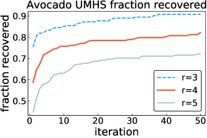
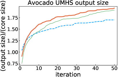
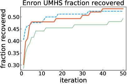
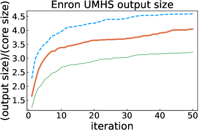
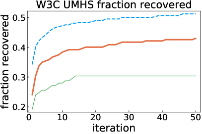
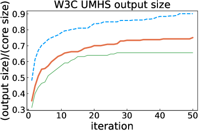
Our UMHS algorithm (Algorithm 2) has a single tuning parameter, which is the number of iterations , i.e., the number of calls to the sub-routine for greedy maximal matching (Algorithm 1). Here we examine performance of UMHS as a function of . Specifically, we analyze (i) the fraction of core nodes in the planted hitting set that are recovered and (ii) the output size of Algorithm 2 as a function of the number of iterations (Fig. 3 shows results for the email datasets).
We highlight a couple of important findings. First, we only need around 50 iterations to achieve high recovery rates. Each iteration is fast, and the entirety of the algorithm’s running time takes at most a few minutes on the larger datasets. Second, the union of minimal hitting sets size tends to increase sharply with a few iterations and then levels off sharply. These results are consistent with our theory. Theorems 3 and 10 both provide theoretical justification for why the output should not grow too large.
5. Related work
On the theoretical side, our problem can be thought of as an instance of a “planted” problem, where a certain type of graph structure is planted or hidden in an a graph and one must recover the latent structure given the graph. Well-studied problems in this space include the planted clique, where one tries to find a clique placed in a sample from a graph (Alon et al., 1998; Feige and Krauthgamer, 2000; Dekel et al., 2011; Deshpande and Montanari, 2014); and the planted partition or stochastic block model recovery, where a random graph is sampled with probabilities dependent on latent labels of nodes, and the goal is to recover these labels (Mossel et al., 2014; Tsourakakis, 2015; Peixoto, 2017; Abbe, 2018). These planted problems are based on some random way in which the graph was sampled. In our case of planted hitting sets, the graph was deterministic, although we could improve our results under a random hypergraph model. Most related to our results is recent work in planted vertex covers; this is a special case of hitting sets for the case of graphs (which mathematically are the same as 2-uniform hypergraphs) (Benson and Kleinberg, 2018b). As discussed above, the hypergraph model is more realistic for many datasets (especially email), given its ability to represent groups of more than two individuals at a time.
Within the field of network science, the idea of a small planted hitting set fits with two related ideas: node centrality and core-periphery structure. The former concept deals with finding important nodes (or ranking them) based on their connections, often provided as a graph (Bonacich, 1987; Boldi and Vigna, 2014; Gleich, 2015). Nodes in hitting sets are central to hypergraphs almost by definition—every hyperedge must contain at least one of these nodes. Thus, we expect them to be “central” in some sense. However, we found that existing measures of node centrality in hypergraphs did not recover planted hitting sets at the same levels as our union of minimal hitting sets algorithm.
Core-periphery structure is a mesoscale property of many networks, where there is a densely connected core set of nodes along with a loosely connected periphery (Csermely et al., 2013). Such a composition has been studied in sociology (Lorrain and White, 1971; Doreian, 1985) and international trade (Smith and White, 1992), where the core-periphery structure is due to differential status. Now, core-periphery identification is a broader tool for identifying structure in general networks (Holme, 2005; Rombach et al., 2017; Govindan et al., 2017; Sarkar et al., 2018). The planted hitting set that we aim to recover corresponds to an extreme type of core-periphery structure; due to the way in which we assume the hypergraph is measured, nodes on the periphery (the “fringe nodes”) cannot be connected without a core node as an intermediary in a hyperedge.
Finally, core-fringe structure itself has received some attention. Romero et al. analyzed the behavior of a core group of employees at a hedge fund in the context of their relationships with contacts outside of the company (Romero et al., 2016), and Benson and Kleinberg analyzed how links between core and fringe nodes influence graph-based link prediction algorithms (Benson and Kleinberg, 2018a). Our research highlights additional richness to the problem when the underlying data model is a hypergraph.
6. Discussion
Network data is a partial view of a larger system (Laumann et al., 1989). A common case is when the interactions of some specified set of actors or nodes are under surveillance. This provides a “core-fringe” structure to the network—we can see all interactions involving the core but only the interactions of the fringe with the core. When data is leaked or metadata is lost over time due to data provenance issues, we would like to be able to recover these core and fringe labels for security or data maintenance purposes.
Here, we have studied this problem where the network data is a hypergraph, so the core is a hitting set. This setting is common in email data or situations in which groups of people are meeting. We used co-authorship as a proxy for the latter situation, but one can imagine situations in which one records the groups of attendees of meetings involving someone under surveillance. Theoretically, we showed that the union of minimal hitting sets cannot be too large and that the output of the well-known approximation algorithm for minimum hitting sets has to somehow overlap the core.
Using these results as motivation, we developed an extremely simple algorithm for recovering the core: take the union of minimal hitting sets that are output by randomly initialized instances of the approximation algorithm. This method out-performed several strong baselines, including methods based on centrality and core-periphery structure.
However, our simple algorithm opens several avenues for improvement in future work. For instance, our model assumed an undirected and unweighted hypergraph structure. There are models of directed and weighted hypergraphs (Gallo et al., 1993) that could be used to improve the recovery algorithm. In addition, theory on the number of calls to the approximation algorithm subroutine would be useful. In practice, only a few calls is sufficient and perhaps assuming particular structure on the hypergraph could yield additional theoretical insight.
References
- (1)
- Abbe (2018) Emmanuel Abbe. 2018. Community Detection and Stochastic Block Models: Recent Developments. JMLR (2018).
- Alon et al. (1998) Noga Alon, Michael Krivelevich, and Benny Sudakov. 1998. Finding a Large Hidden Clique in a Random Graph. In SODA.
- Benson (2018) Austin R Benson. 2018. Three hypergraph eigenvector centralities. arXiv:1807.09644 (2018).
- Benson et al. (2018) Austin R. Benson, Rediet Abebe, Michael T. Schaub, Ali Jadbabaie, and Jon Kleinberg. 2018. Simplicial closure and higher-order link prediction. PNAS (2018).
- Benson and Kleinberg (2018a) Austin R Benson and Jon Kleinberg. 2018a. Core-fringe link prediction. arXiv:1811.11540 (2018).
- Benson and Kleinberg (2018b) Austin R. Benson and Jon Kleinberg. 2018b. Found Graph Data and Planted Vertex Covers. In NeurIPS.
- Boldi et al. (2004) Paolo Boldi, Bruno Codenotti, Massimo Santini, and Sebastiano Vigna. 2004. UbiCrawler: a scalable fully distributed Web crawler. Software: Practice and Experience (2004).
- Boldi et al. (2014) Paolo Boldi, Andrea Marino, Massimo Santini, and Sebastiano Vigna. 2014. BUbiNG: Massive Crawling for the Masses. In WWW.
- Boldi and Vigna (2014) Paolo Boldi and Sebastiano Vigna. 2014. Axioms for Centrality. Internet Mathematics (2014).
- Bollobás (1986) Béla Bollobás. 1986. Combinatorics: set systems, hypergraphs, families of vectors, and combinatorial probability. Cambridge University Press.
- Bonacich (1987) Phillip Bonacich. 1987. Power and Centrality: A Family of Measures. American J. of Sociology (1987).
- Borgatti and Everett (2000) Stephen P Borgatti and Martin G Everett. 2000. Models of core/periphery structures. Social Networks (2000).
- Buneman et al. (2001) Peter Buneman, Sanjeev Khanna, and Tan Wang-Chiew. 2001. Why and Where: A Characterization of Data Provenance. In ICDT.
- Craswell et al. (2005) Nick Craswell, Arjen P de Vries, and Ian Soboroff. 2005. Overview of the TREC 2005 Enterprise Track. In TREC, Vol. 5. 199–205.
- Csermely et al. (2013) P. Csermely, A. London, L.-Y. Wu, and B. Uzzi. 2013. Structure and dynamics of core/periphery networks. J. of Complex Networks (2013).
- Damaschke (2006) Peter Damaschke. 2006. Parameterized enumeration, transversals, and imperfect phylogeny reconstruction. Theoretical Computer Science (2006).
- Damaschke and Molokov (2009) Peter Damaschke and Leonid Molokov. 2009. The union of minimal hitting sets: Parameterized combinatorial bounds and counting. J. of Discrete Algorithms (2009).
- Davis and Goadrich (2006) Jesse Davis and Mark Goadrich. 2006. The relationship between Precision-Recall and ROC curves. In ICML.
- Dekel et al. (2011) Yael Dekel, Ori Gurel-Gurevich, and Yuval Peres. 2011. Finding Hidden Cliques in Linear Time with High Probability. In ANALCO.
- Deshpande and Montanari (2014) Yash Deshpande and Andrea Montanari. 2014. Finding Hidden Cliques of Size in Nearly Linear Time. Foundations of Computational Mathematics (2014). https://doi.org/10.1007/s10208-014-9215-y
- Doreian (1985) Patrick Doreian. 1985. Structural equivalence in a psychology journal network. J. of the American Society for Information Science (1985).
- Erdös and Rado (1960) Paul Erdös and Richard Rado. 1960. Intersection theorems for systems of sets. J. of the London Mathematical Society (1960).
- Feige and Krauthgamer (2000) Uriel Feige and Robert Krauthgamer. 2000. Finding and certifying a large hidden clique in a semirandom graph. Random Structures and Algorithms (2000).
- Gallo et al. (1993) Giorgio Gallo, Giustino Longo, Stefano Pallottino, and Sang Nguyen. 1993. Directed hypergraphs and applications. Discrete Applied Mathematics (1993).
- Ghoshdastidar and Dukkipati (2014) Debarghya Ghoshdastidar and Ambedkar Dukkipati. 2014. Consistency of spectral partitioning of uniform hypergraphs under planted partition model. In NeurIPS.
- Gile and Handcock (2010) Krista J. Gile and Mark S. Handcock. 2010. Respondent-Driven Sampling: An Assessment of Current Methodology. Sociological Methodology (2010).
- Gleich (2015) David F. Gleich. 2015. PageRank Beyond the Web. SIAM Rev. (2015).
- Goel and Salganik (2010) S. Goel and M. J. Salganik. 2010. Assessing respondent-driven sampling. PNAS (2010).
- Govindan et al. (2017) Priya Govindan, Chenghong Wang, Chumeng Xu, Hongyu Duan, and Sucheta Soundarajan. 2017. The k-peak Decomposition. In WWW.
- Guimerà and Sales-Pardo (2009) Roger Guimerà and Marta Sales-Pardo. 2009. Missing and spurious interactions and the reconstruction of complex networks. PNAS (2009).
- Halldórsson and Losievskaja (2009) Magnús M. Halldórsson and Elena Losievskaja. 2009. Independent sets in bounded-degree hypergraphs. Discrete Applied Mathematics (2009).
- Heckathorn (2011) Douglas D. Heckathorn. 2011. Comment: Snowball versus Respondent-Driven Sampling. Sociological Methodology (2011).
- Hier and Greenberg (2009) Sean P. Hier and Josh Greenberg. 2009. Surveillance: Power, Problems, and Politics. UBC Press.
- Holme (2005) Petter Holme. 2005. Core-periphery organization of complex networks. PRE (2005).
- Kapoor et al. (2013) Komal Kapoor, Dhruv Sharma, and Jaideep Srivastava. 2013. Weighted node degree centrality for hypergraphs. In IEEE Network Science Workshop.
- Klimt and Yang (2004) Bryan Klimt and Yiming Yang. 2004. The Enron Corpus: A New Dataset for Email Classification Research. In Machine Learning: ECML 2004.
- Kossinets (2006) Gueorgi Kossinets. 2006. Effects of missing data in social networks. Social Networks (2006).
- Kostochka et al. (2014) Alexandr Kostochka, Dhruv Mubayi, and Jacques Verstraëte. 2014. On independent sets in hypergraphs. Random Structures & Algorithms (2014).
- Kuny (1997) T Kuny. 1997. A digital dark ages? Challenges in the preservation of electronic information of electronic information. In IFLA Council and General Conference.
- Laumann et al. (1989) Edward O Laumann, Peter V Marsden, and David Prensky. 1989. The boundary specification problem in network analysis. Research methods in social network analysis (1989).
- Lorrain and White (1971) François Lorrain and Harrison C. White. 1971. Structural equivalence of individuals in social networks. The J. of Mathematical Sociology (1971).
- Lynch (2008) Clifford Lynch. 2008. How do your data grow? Nature (2008).
- Mossel et al. (2014) Elchanan Mossel, Joe Neeman, and Allan Sly. 2014. Belief propagation, robust reconstruction and optimal recovery of block models. In COLT.
- Peixoto (2017) Tiago P. Peixoto. 2017. Nonparametric Bayesian inference of the microcanonical stochastic block model. PRE (2017).
- Rombach et al. (2017) Puck Rombach, Mason A. Porter, James H. Fowler, and Peter J. Mucha. 2017. Core-Periphery Structure in Networks (Revisited). SIAM Rev. (2017).
- Romero et al. (2016) Daniel M. Romero, Brian Uzzi, and Jon Kleinberg. 2016. Social Networks Under Stress. In WWW.
- Sarkar et al. (2018) Soumya Sarkar, Sanjukta Bhowmick, and Animesh Mukherjee. 2018. On Rich Clubs of Path-Based Centralities in Networks. In CIKM.
- Seidman (1983) Stephen B. Seidman. 1983. Network structure and minimum degree. Social Networks (1983).
- Simmhan et al. (2005) Yogesh L. Simmhan, Beth Plale, and Dennis Gannon. 2005. A survey of data provenance in e-science. ACM SIGMOD Record (2005).
- Smith and White (1992) D. A. Smith and D. R. White. 1992. Structure and Dynamics of the Global Economy: Network Analysis of International Trade 1965–1980. Social Forces (1992).
- Tan (2004) Wang-Chiew Tan. 2004. Research problems in data provenance. IEEE Data Engineering Bulletin (2004).
- Tsiatas et al. (2013) Alexander Tsiatas, Iraj Saniee, Onuttom Narayan, and Matthew Andrews. 2013. Spectral analysis of communication networks using Dirichlet eigenvalues. In WWW.
- Tsourakakis (2015) Charalampos Tsourakakis. 2015. Streaming Graph Partitioning in the Planted Partition Model. In COSN.