Visual binary stars with partially missing data: Introducing multiple imputation in astrometric analysis

Abstract

Partial measurements of relative position are a relatively common event during the observation of visual binary stars. However, these observations are typically discarded when estimating the orbit of a visual pair. In this article we present a novel framework to characterize the orbits from a Bayesian standpoint, including partial observations of relative position as an input for the estimation of orbital parameters. Our aim is to formally incorporate the information contained in those partial measurements in a systematic way into the final inference. In the statistical literature, an imputation is defined as the replacement of a missing quantity with a plausible value. To compute posterior distributions of orbital parameters with partial observations, we propose a technique based on Markov chain Monte Carlo with multiple imputation. We present the methodology and test the algorithm with both synthetic and real observations, studying the effect of incorporating partial measurements in the parameter estimation. Our results suggest that the inclusion of partial measurements into the characterization of visual binaries may lead to a reduction in the uncertainty associated to each orbital element, in terms of a decrease in dispersion measures (such as the interquartile range) of the posterior distribution of relevant orbital parameters. The extent to which the uncertainty decreases after the incorporation of new data (either complete or partial) depends on how informative those newly-incorporated measurements are. Quantifying the information contained in each measurement remains an open issue.

1 Introduction

Incomplete or missing data is not uncommon in observational astronomy and, indeed, partial measurements are a relatively common phenomenon when doing astrometry of visual binary stars. Usually, this phenomenon does not derive from random data loss (as occurs in communication systems, for example), but rather from the impossibility of resolving the relative position between components on an image or sequence of images, e.g., in speckle interferometry, the maximum angular resolution for detection of a companion may depend on a number of factors such as the magnitude difference between the pairs (see, e.g., Figure 5 in Tokovinin (2018)). Images of visual pairs, obtained by means of optical telescopes or interferometric techniques, are expected to display each component as a sharp point over a fainter background, thus enabling the viewer to identify their position in the plane of the sky. However, a number of factors may hinder the process of resolving a binary star: excessive or insufficient exposure time of the imaging devices, presence of additional noise due to atmospheric conditions, varying degrees of brightness of the objects being observed, angular separations beyond the angular resolution of the telescope, etc. The latter case is arguably the most common source of partial information: in the vicinity of the periastron, the angular separation between the primary and secondary star (denoted by $\rho$ hereafter) reaches its minimum values; if those values fall below the resolution threshold of the imaging device, then the angular separation is confined to a range (i.e., $\rho\in(0,\rho_{\textrm{max}})$) instead of being reduced to a single value (as occurs with regular, successfully resolved measurements), and usually no information about the position angle of the secondary with respect to the primary (denoted by $\vartheta$ hereafter) can be inferred either. In certain cases, databases of visual binary observations also report partial data of the form $\rho=(0,\infty)$, $\vartheta=\vartheta^{\ast}$, that is, the angular separation is missing but the position angle is well-defined. Many example of partially missing data (in $\rho$ or $\vartheta$) can be found by browsing either through the historical measurements database of the Washington Double Star Catalogue (WDS hereafter, Mason et al. (2001)) or the Catalog of Interferometric Measurements of Binary Stars (INT hereafter, Hartkopf et al. (2001)), both diligently curated by the Naval Observatory of the United States.

In a broader context, from population censuses to clinical research surveys, the presence of incomplete or missing data may occur in a wide range of statistical situations (a more in-depth introduction to be problem can be found in Dempster et al. (1977) and Little & Rubin (2002), Chapter 1). Since standard inference methods are conceived to be used with complete data sets, missing values imply a challenge for data analysts. Several approaches can be taken to deal with partial or missing data. The most naive strategy is to discard data entries with partial measurements (with the information contained in them remaining unused), and then apply a standard technique on the subset of complete measurements or, in the best of cases, to use the partial information only in a qualitative assesment of the solution. However, the validity and efficiency of complete-data based methods cannot be guaranteed when data are incomplete (Rubin, 1976). In the particular case of visual binaries, the incorporation of incomplete data, however, may have the potential to reduce the uncertainty about orbital parameters. A hint of that can be appreciated in the fact that some astronomers use partial data in a somewhat subjective way: incomplete entries are not included as an input of the estimation routines (whichever they might be: least-squares methods, Markov chain Monte Carlo, etc.); however, within a set of orbit proposals (obtained by means of complete data), the solutions that violate the ranges imposed by partial information can be rejected (for example, if $\rho$ is known to be in $(0,\rho_{\textrm{max}})$ for certain epoch, but the model predicts an angular separation significantly larger than $\rho_{\textrm{max}}$). Our conjecture on this is that partial measurements may be useful in certain observational conditions, and that the Bayesian approach offers a proper statistical framework to include this data and improve the estimation of orbital parameters.

Due to its relevance for the calculation of stellar masses, the problem of estimating orbital parameters based on observations of relative positions of visual binary stars has been largely studied in the astronomical community. From geometry-based procedures such as the Thiele-Innes-Van den Bos method (Thiele, 1883) or Docobo (1985) to modern Bayesian techniques such as those presented in Ford (2005), Lucy (2014), or Sahlmann et al. (2013) (to mention a few), orbit fitting has been addressed from a wide range of approaches. However, the issue of partial measurements in orbital estimation has been systematically ignored. This work presents a novel extension of our previous Markov chain Monte Carlo-based method to estimate orbital parameters (Mendez et al. (2017)), that fully incorporates partial data into the inference using an imputation approach. The cases addressed are those mentioned in the preceding paragraph, namely, $\rho\in(0,\rho_{\textrm{max}}),\vartheta\in(0,2\pi)$ and $\rho\in(0,\infty)$, $\vartheta=\vartheta^{\ast}$. Entries where a Cartesian coordinate is missing, as well as cases where the feasible zone of the missing observation has an arbitrary geometry, are theoretical possibilities; however, they are not addressed in this work, since they do not usually occur in real situations. To the best of our knowledge, this is the first time that this technique of multiple imputation is applied to the estimation of orbital parameters. For a brief account of the use of this technique in the wider field of astronomy, see Chattopadhyay & Chattopadhyay (2014), Chapter 6.

The structure of our paper is as follows: In Section 2 we introduce the basic concepts of imputation theory and how this can be implemented through a Markov chain Monte Carlo approach in a very generic setting. Then, in Section 3 we bring down to earth (or rather, to the heavens), the concepts outlined in the previous section by describing the methodology for our specific application: computing orbital elements of visual binaries using partial data. In Sections 4 and 5 we present the results of applying our imputation methodology to a controlled (simulated) experiment, and to a real test case for the visual binary HU177 respectively. Finally in Section 6 we present our main conclusions. Appendices A and B provide further details regarding the solution of the orbital elements and the pseudo-codes used, which can be made available in full upon request to the main author. Appendix C contains relevant details on the technical aspects of the Markov chain Monte Carlo (MCMC hereinafter) techniques used in this work: chain convergence, initialization and burn-in period.

2 Multiple imputation theory and implementation

2.1 A premier on multiple imputation

A number of techniques specifically aimed at addressing the problem of missing or partial measurements have been proposed. For example, Dempster et al. (1977) use an Expectation-Maximization (EM hereinafter) algorithm to calculate maximum likelihood estimates from incomplete data. Another approach is to fill in the blank spaces due to missing data with plausible values –referred to as imputations–, thus generating a set of observations on which standard complete-data based methods can be applied. Regardless of the specific manner in which imputations are generated, methods that proceed like that can be labeled as “single imputation techniques”. Both EM and single imputation techniques have certain drawbacks: EM is not suitable when the object of interest is the likelihood or posterior distribution rather than just a maximizer (and the curvature at that point, at most); on the other hand, single imputation techniques omit the sources of uncertainty associated to the imputation process, which may lead to biased results. These sources of uncertainty are enumerated as follows: One is the uncertainty associated to the modelling of the joint distribution of the response variables $\mathcal{Y}$ (observed and unobserved) and the missingness indicator $R$ (see Equation (2)); the second is the uncertainty of the imputation model, assuming that values of the observed data and the model parameters are known (associated with the term later identified as conditional predictive distribution, see the first term inside the integral in Equation (3)); the third is the uncertainty about the model parameters (denoted by $\theta$ in what follows) themselves, i.e., $p(\theta|\mathcal{Y})$ (Zhang, 2003). Further details are explained throughout this section.

Introduced by Rubin (1987), the approach known as multiple imputation is aimed at performing inference from incomplete data while taking into account the uncertainty sources that single imputation techniques ignore. Multiple imputation relies on replacing missing values with not one, but multiple plausible values, thus generating several complete data sets which differ from each other only in the imputed values–entries with complete data remain the same. These data sets are analyzed individually with standard techniques and the final inference is performed by combining the individual results (e.g., by calculating an average).

At this point, certain definitions must be introduced in order to formalize the problem of missing data and the techniques to address it. Let $\mathcal{Y}$ be an observation matrix, with each row $y_{i}$ being a single multivariate observation of a certain dimension drawn from a probability distribution $p(y|\theta)$ governed by the model parameter vector $\theta$ (in the application to visual binary stars the dimension of $y_{i}$ would be two, corresponding to the angular separation between the components, and the position angle of the secondary with respect to the primary, whereas the vector $\theta$ will have as its components the seven orbital parameters, see Section 3.1). The components of the missingness indicator matrix $R$ are defined as:

$$r_{ij}=\begin{cases}0\text{ if }y_{ij}\text{ is observed},\\ 1\text{ if }y_{ij}\text{ is missing}.\end{cases}$$ (1)

Defining the probability of $r_{ij}=0$ given $y_{ij}$ as $p_{ij}$ (conversely, the probability of $r_{ij}=1$ given $y_{ij}$ would be $1-p_{ij}$), the value of $R$ is subject to a probability distribution $p(R|\xi,\mathcal{Y})$ which depends on parameters $\xi$ (i.e., $\xi$ encodes the set of rules that define the matrix $R$). Thus, by virtue of the chain rule of probability, the joint distribution of $\mathcal{Y}$ and $R$ can be expressed as:

$$p(\mathcal{Y},R|\theta,\xi)=p(\mathcal{Y}|\theta)\cdot p(R|\xi,\mathcal{Y}),$$ (2)

where the term $p(\mathcal{Y}|\theta)$ is the conditional distribution of the observations given the model parameters. It has been assumed that $p(\mathcal{Y}|\theta,\xi)=p(\mathcal{Y}|\theta)$ and that $p(R|\xi,\theta,\mathcal{Y})=p(R|\xi,\mathcal{Y})$. Values within $\mathcal{Y}$ can be split into $\mathcal{Y}_{\textrm{mis}}$ (values in $\mathcal{Y}$ such that $r_{ij}=1$) and $\mathcal{Y}_{\textrm{obs}}$ (values in $\mathcal{Y}$ such that $r_{ij}=0$). Since the conclusions about the target parameters $\theta$ must be based on the joint probability model (Equation (2)), the manner in which the missingness depends on $\mathcal{Y}$ must be taken into account when performing inference. Little & Rubin (2002) identified three missingness mechanisms:

• Missing completely at random (MCAR): $p(R|\xi,(\mathcal{Y}_{\textrm{mis}},\mathcal{Y}_{\textrm{obs}}))=p(R|\xi)$. For example, in a clinical trial participants would flip a coin to decide whether they fill in a depression survey,

• Missing at random (MAR): $p(R|\xi,(\mathcal{Y}_{\textrm{mis}},\mathcal{Y}_{\textrm{obs}}))=p(R|\xi,\mathcal{Y}_{\textrm{obs}})$, i.e., the occurrence of data loss depends only on the observed values. Following the example above, male participants could be more likely to refuse to complete the depression survey, regardless their individual levels of depression (“they tend to skip the survey just because they are male”), and,

• Missing not at random (MNAR): $p(R|\xi,(\mathcal{Y}_{\textrm{mis}},\mathcal{Y}_{\textrm{obs}}))\neq p(R|\xi,\mathcal{Y}_{\textrm{obs}})$, that is, the occurrence of data loss may depend on unobserved values. In the clinical trial mentioned above, male participants might be more reluctant to complete the survey as their level of depression is higher (“they tend to skip the survey because they are depressed”).

The terms $\theta$ and $\xi$ are said to be distinct if their joint probability can be expressed as a product of independent marginal probability density functions (PDFs hereinafter) (Rubin, 1976). If that condition holds, and if either MCAR or MAR applies, inferences based on the observed-data likelihood function $L(\theta,\xi|\mathcal{Y}_{\textrm{obs}},R)$ will be the same as those based on $L(\theta|\mathcal{Y}_{\textrm{obs}})$. In those cases, the missingness mechanism is said to be ignorable. However, the precision of the inference thus performed is reduced if a large portion of the information is missing – this is precisely what motivates the multiple imputation approach.

The conditional probability of $\mathcal{Y}_{\textrm{mis}}$ given $\mathcal{Y}_{\textrm{obs}}$ can be obtained by integrating over the parameter space of $\theta$, that is:

$$p(\mathcal{Y}_{\textrm{mis}}|\mathcal{Y}_{\textrm{obs}})=\int p(\mathcal{Y}_{\textrm{mis}}|\mathcal{Y}_{\textrm{obs}},\theta)\,p(\theta|\mathcal{Y}_{\textrm{obs}})\,d\theta.$$ (3)

Following the terminology proposed by Zhang (2003), the term $p(\mathcal{Y}_{\textrm{mis}}|\mathcal{Y}_{\textrm{obs}},\theta)$ is identified as the conditional predictive distribution of $\mathcal{Y}_{\textrm{mis}}$ given $\mathcal{Y}_{\textrm{obs}}$ and $\theta$. The term $p(\mathcal{Y}_{\textrm{mis}}|\mathcal{Y}_{\textrm{obs}})$ is identified as the posterior predictive distribution of $\mathcal{Y}_{\textrm{mis}}$ given $\mathcal{Y}_{\textrm{obs}}$, and must be understood as the conditional predictive distribution averaged over the observed-data posterior distribution of $\theta$, $p(\theta|\mathcal{Y}_{\textrm{obs}})$. Although $p(\mathcal{Y}_{\textrm{mis}}|\mathcal{Y}_{\textrm{obs}})$ is seldom found in a closed form, expressions for both $p(\mathcal{Y}_{\textrm{mis}}|\mathcal{Y}_{\textrm{obs}},\theta)$ and $p(\theta|\mathcal{Y}_{\textrm{obs}})$ may be found in certain situations. On the other hand, $p(\mathcal{Y}_{\textrm{mis}}|\mathcal{Y}_{\textrm{obs}},\theta)$ depends on the imputation model adopted. Examples of standard imputation models existing in the literature are the predictive model method (Little & Rubin, 2002) and the propensity score method (Lavori et al., 1995), which are only applicable when data follows a monotone missing pattern.

Let $Q$ be any quantity of interest to be estimated from the observed data. Then, the core of the multiple imputation approach is the estimation of $Q$ by averaging the completed-data posterior, $p(Q|\mathcal{Y}_{\textrm{obs}},\mathcal{Y}_{\textrm{mis}})$, over the feasible values of $\mathcal{Y}_{\textrm{mis}}$ given $\mathcal{Y}_{\textrm{obs}}$ (which are represented by the distribution $p(\mathcal{Y}_{\textrm{mis}}|\mathcal{Y}_{\textrm{obs}})$ and depend, ultimately, on the chosen imputation model):

$$p(Q|\mathcal{Y}_{\textrm{obs}})=\int p(Q|\mathcal{Y}_{\textrm{obs}},\mathcal{Y}_{\textrm{mis}})\,p(\mathcal{Y}_{\textrm{mis}}|\mathcal{Y}_{\textrm{obs}})\,d\mathcal{Y}_{\textrm{mis}}.$$ (4)

This integral can be approximated as the discrete average of the values of $Q$ obtained from a finite, possibly small, number of data sets filled in with imputations. Zhang (2003) presents a detailed discussion of how the number of imputations affects the estimation variance.

2.2 MCMC for multiple imputation

Markov chain Monte Carlo, usually shortened to MCMC, designates a wide class of sampling techniques that rely on constructing a Markov chain whose equilibrium distribution is the same as that from which one desires to sample. The chain is designed to explore the domain of the target distribution (in this case, orbital elements) in such a way that it spends most of the time in areas of high probability (Andrieu et al., 2003). Since the implementation of the algorithm is essentially independent of the target distribution, MCMC provides a means to efficiently draw samples from distributions with complex analytic formulae and/or multidimensional domains. Furthermore, MCMC does not require a complete knowledge of the target distribution $p(X)$, but just being able to evaluate $p(X)$ up to a normalizing constant ($X$ refers to a generic variable of interest, in our case $X=\theta$). For a thorough introduction to this technique, see the textbooks (Brooks et al., 2011; Gelman et al., 2013).

Introduced in Metropolis & Ulam (1949), Metropolis et al. (1953) and subsequently generalized to a larger class of algorithms in Hastings (1970), MCMC techniques have been applied to a wide range of problems, such as statistical mechanics, optimization or –most relevant to this work– Bayesian inference (Andrieu et al., 2003). Within the field of astronomy, Bayesian inference has become somewhat of a standard approach in the exoplanet research community since the seminal works of Ford (2005) and Gregory (2005), where the authors address the problem of estimating the orbital parameters of an exoplanet from a Bayesian perspective and use MCMC to approximate their posterior distribution. In the last decade, besides making up an important part of the Kepler Mission data processing pipeline (Rowe et al., 2014; Gautier III et al., 2012), recent findings such as the celebrated discovery of seven temperate terrestrial planets orbiting the ultra-cool dwarf star TRAPPIST-$1$ (Gillon et al., 2017) relied to some extent on MCMC. Its use in the characterization of orbits of binary stars, however, has been more limited, despite the high degree of formal similarity between exoplanets and multiple stellar sysrtems. Some examples of works addressing the estimation of orbital parameters of binary stars from a Bayesian perspective (but only using complete datasets) are Sahlmann et al. (2013); Burgasser et al. (2015) and Mendez et al. (2017).

When data loss is not governed by a monotone pattern, imputation models such as the predictive model method and the propensity score method cannot be applied. To input the missing values in cases with arbitrary missing patterns, more advanced techniques must be adopted. The data augmentation algorithm introduced in Tanner & Wong (1987), which is formally an MCMC method, stems as a useful tool for those cases.

The data augmentation algorithm is motivated by the representation of the desired posterior distribution found in Equation (4), where the quantity of interest $Q$ is typically a parameter vector $\theta$. The term $p(\theta|\mathcal{Y}_{\textrm{obs}})$ depends, in turn, on $p(\mathcal{Y}_{\textrm{mis}}|\mathcal{Y}_{\textrm{obs}})$. Tanner & Wong (1987) prove, by using a fixed point-based argument, that under mild conditions the following scheme converges to $p(\theta|\mathcal{Y}_{\textrm{obs}})$:

1. Generate $\mathcal{Y}_{\textrm{mis}}^{(i,1)},\dots,\mathcal{Y}_{\textrm{mis}}^{(i,m)}$ from the current approximation of the predictive posterior distribution, $p_{i}(\mathcal{Y}_{\textrm{mis}}|\mathcal{Y}_{\textrm{obs}})$. This can be accomplished by, first, drawing a sample $\theta_{i}$ from $p_{i}(\theta|\mathcal{Y}_{\textrm{obs}})$; and, then, sampling $m$ values of $\mathcal{Y}_{\textrm{mis}}$ from $p(\mathcal{Y}_{\textrm{mis}}|\theta_{i},\mathcal{Y}_{\textrm{obs}})$,

2. Update the approximation of the desired posterior PDF, $p_{i}(\theta|\mathcal{Y}_{\textrm{obs}})$, by averaging the results obtained from the completed data sets:

   $$p_{i+1}(\theta|\mathcal{Y}_{\textrm{obs}})=\frac{1}{m}\sum_{j=1}^{m}p(\theta|\mathcal{Y}_{\textrm{mis}}^{(i,j)},\mathcal{Y}_{\textrm{obs}})$$ (5)

3. If a stopping criterion has been reached, stop. If not, return to step $1$.

Steps 1 and 2 are referred to as I-step (Imputation step) and P-step (Posterior step), respectively, in analogy to the Expectation and Maximization steps of the EM algorithm. The evaluation of the function $p(\theta|\mathcal{Y}_{\textrm{mis}},\mathcal{Y}_{\textrm{obs}})$ in step $2$ is replaced by a sampling procedure in certain situations (e.g., if $p(\theta|\mathcal{Y}_{\textrm{mis}},\mathcal{Y}_{\textrm{obs}})$ is known up to constant, if the distribution is not known in a closed form but it is possible to sample from it, etc.).

Figure 1: Algorithm 1: MCMC pseudo-code for multiple imputation

Tanner & Wong (1987) have suggested that even a value as small as $m=1$ in Equation (5) leads to a correct approximation, in the sense that the average of the posterior distribution across the iterations –the one obtained in the step 2– will converge to $p(\theta|\mathcal{Y}_{\textrm{obs}})$. This motivates the MCMC scheme actually used in later publications on missing data (Zhang, 2003) and available on some commercial software implementations (see, e.g., Yuan (2010)). This method is described in Algorithm 1: by following this scheme during a sufficiently large number of iterations, one obtains a sequence $\{\theta^{(i)},\mathcal{Y}_{\textrm{mis}}^{(i)}\}_{i=0,\cdots,N_{\textrm{steps}}}$ whose stationary distribution is $p(\theta,\mathcal{Y}_{\textrm{mis}}|\mathcal{Y}_{\textrm{obs}})$. The chain length, $N_{\textrm{steps}}$, is determined empirically based on the desired precision of the estimated parameters. Marginalizing out $\mathcal{Y}_{\textrm{mis}}$ yields the desired posterior distribution $p(\theta|\mathcal{Y}_{\textrm{obs}})$, whereas by marginalizing out $\theta$ one obtains the posterior predictive distribution $p(\mathcal{Y}_{\textrm{mis}}|\mathcal{Y}_{\textrm{obs}})$. Note that $\theta^{(i)}$ is sampled from $p(\theta|\mathcal{Y}_{\textrm{mis}}^{(i)},\mathcal{Y}_{\textrm{obs}})$ instead of $p(\theta|\mathcal{Y}_{\textrm{obs}})$, since, given that $m=1$, the averaging step described by Equation (5) is not performed.

3 Methodology as applied to visual binary stars

This section details the implementation of the general technique described in Section 2 applied to the problem of orbital estimation. Section 3.1 briefly introduces the model adopted to mathematically characterize the movement of a binary star. Section 3.2 provides a background on the use of MCMC for parameter estimation, and details the implementation used in this work. Finally, Section 3.3 presents the details on how the generic imputation algorithm presented in Section 2.2 is adapted to the specific problem addressed in this work.

3.1 Dynamics of a binary star

Under the assumption that phenomena such as mass transfer, relativistic effects or the presence of non-visible additional bodies do not occur, or have a negligible consequences, we adopt a Keplerian model to characterize the movement of binary stars. This model requires seven parameters–the well-known Campbell elements shown in Equation (6)–to compute the relative position of the two components of a binary star for any given epoch $\tau$, namely:

$$\theta=\{P,T,e,a,\omega,\Omega,i\},\\$$ (6)

where $P$, $T$, $e$ correspond to orbital period, time of periastron passage, and eccentricity respectively; $a$ denotes the semi-major axis of the elliptical orbit, and the angular parameters $\omega$, $\Omega$, and $i$ indicate the spatial orientation of the orbit from the point of the view of the observer. Details about these parameters, as well as a complete derivation of the Keplerian model, can be consulted e.g., in Van de Kamp & Stearns (1967).

Calculating the position $(\rho,\vartheta)$ of the relative orbit (or the equivalent Cartesian coordinates ($X$, $Y$)) at a certain instant of time $\tau$ involves a sequence of steps, described in what follows:

• Solving Kepler’s equation in order to obtain the eccentric anomaly $E$:

  $$M=2\pi(\tau-T)/P=E-e\sin E.$$ (7)

• Computing the auxiliary values $x$, $y$, referred to as normalized coordinates hereinafter:

  $$x(E) =\cos E-e,$$ (8)

  $$y(E) =\sqrt{1-e^{2}}\sin E.$$

• Determining the Thiele-Innes constants:

  $$A= ~{}a(\cos\omega~{}\cos\Omega-\sin\omega~{}\sin\Omega~{}\cos i),$$ (9)

  $$B= ~{}a(\cos\omega~{}\sin\Omega+\sin\omega~{}\cos\Omega~{}\cos i),$$

  $$F= ~{}a(-\sin\omega~{}\cos\Omega-\cos\omega~{}\sin\Omega~{}\cos i),$$

  $$G= ~{}a(-\sin\omega~{}\sin\Omega+\cos\omega~{}\cos\Omega~{}\cos i).$$

• Calculating the position in the apparent orbit as:

  $$X =Bx+Gy$$ (10)

  $$Y =Ax+Fy.$$

By virtue of the Thiele-Innes representation, where the parameter set $\{P,T,e,a,\omega,\Omega,i\}$ is replaced by the equivalent $\{P,T,e,A,B,F,G\}$, the dimension of the feature space of this problem is reduced from 7 to 3: by exploiting the linear dependency of the Thiele-Innes constants (Eq. 9) with respect to the normalized coordinates $x$, $y$ (which in turn depend on $P$, $T$, $e$ and epochs of observation $\{\tau_{i}\}_{i=1,\dots,N}$), a least-squares estimate of parameters $A,B,F,G$ can be obtained from the observations directly by simple matrix algebra, a procedure that is outlined in Appendix A. The approach described here is well-known within the astronomical literature, being Hartkopf et al. (1989); Pourbaix (1994); Lucy (2014), and Mendez et al. (2017) some examples of its use.

3.2 Bayesian estimation of orbital parameters

Rather than calculating a point estimate of the orbital elements of a binary star, the Bayesian approach intends to characterize the degree of knowledge about those parameters $\theta$, given a set of observations ($\mathcal{Y}$). This knowledge is represented by a PDF–the posterior parameter distribution $p(\theta|\mathcal{Y})$– which, by virtue of the Bayes theorem (Equation (11)), is the result of upgrading the previous knowledge about the variables of interest–represented by the prior distribution $p(\theta)$–with up-to-date measurements, which modify the current level of knowledge through the likelihood function $p(\mathcal{Y}|\theta)$. The term $p(\mathcal{Y})$ does not depend on $\theta$, and thus is dismissed as a mere normalization constant in sampling applications.

$$p(\theta|\mathcal{Y})=\displaystyle\frac{p(\mathcal{Y}|\theta)\cdot p(\theta)}{P(\mathcal{Y})}.$$ (11)

As mentioned in Section 2.2, calculation of posterior distributions and the integrals associated, such as marginal distributions or expected values, may involve a number of difficulties: multidimensionality, complex analytic formulae, ignorance of the value of a normalization constant, etc. (Andrieu et al., 2001). Thus, the sampling technique briefly introduced in Section 2.2 in the context of partial measurements –MCMC– arises as a practical solution to approximate those quantities. As a necessary background material for Section 3.3, this section explain how MCMC-based approximations of posterior PDFs is implemented in the context of orbital parameters of visual binary stars with complete measurements:

• The parameters of interest are the orbital elements contained in Equation (6). The Thiele-Innes representation is used: $\theta=[P,T,e,B,A,F,G]$, with vector $\theta$ separated into non-linear and linear elements: $\theta_{NL}=[P,T,e]$ (those on which MCMC perform its “exploration”) and $\theta_{L}=[B,A,F,G]$ (calculated by least-squares in the manner described in Appendix A.1). Term $\theta_{L}$ indicates the “linear” section of the vector of orbital parameters, which can be obtained by matrix algebra.

• According to Ford (2005), it is common practice to choose a non-informative prior that is uniform in the logarithm space for positive definite magnitudes (for example, period $P$ and semi-major axis $a$), following certain scaling arguments presented in Gelman et al. (2003). In the context of orbital estimation, this approach has also been used in, for example, Gregory (2005), Sahlmann et al. (2013), and Lucy (2014). It must be noted, however, that using unbounded uniform priors (in either the original or the logarithmic domain) leads to improper distributions. In this work, this problem is circumvented by limiting the domain of the target variable: in sections 5, 4, $P$ values out of the range $[P_{\textrm{min}},P_{\textrm{max}}]~{}yr$ are rejected. From a practical point of view, the $\log P$ representation increases the rate of convergence in systems for which the period is not well constrained. In exploration-based methods such as MCMC, the use of a Gaussian in the logarithm of $P$ as a proposal distribution has been proven to be useful (Gregory (2005)), hence this is the approach adopted in this work.

• The target distribution $f(\cdot)$ of our MCMC routine is the posterior distribution of orbital parameters, $p(\theta|\mathcal{Y})$, which has the canonical form $prior\times likelihood$. Terms from the prior PDF can be dropped, as uniform priors were used for $T$, $\log P$ and $e$. Thus, the likelihood function can be directly utilized to evaluate the Metropolis-Hastings ratio. Assuming individual Gaussian errors for each observation, the likelihood function of a set of parameters $\theta$ is computed as:

  $$f(\theta)=p(\theta|\mathcal{Y})\propto\displaystyle\exp\biggl{(}-\frac{1}{2}\Bigl{(}\sum_{k=1}^{N_{x}}\frac{1}{\sigma_{x}^{2}(k)}[X_{\textrm{obs}}^{(k)}-X_{\textrm{model}}(\theta,\tau_{k})]^{2}+$$

  $$\sum_{k=1}^{N_{y}}\frac{1}{\sigma_{y}^{2}(k)}[Y_{\textrm{obs}}^{(k)}-Y_{\textrm{model}}(\theta,\tau_{k})]^{2}\Bigr{)}\biggr{)},$$ (12)

  where $\mathcal{Y}$ is the set of observed values of relative position ($X_{\textrm{obs}}$, $Y_{\textrm{obs}}$). Terms $\sigma_{x}^{2}(k),~{}\sigma_{y}^{2}(k)$ indicate the measurement errors at epoch $\tau_{k}$. Positions $X_{\textrm{model}}$, $Y_{\textrm{model}}$ are calculated according to $\tau_{k}$ and the parameter values contained in $\theta$, following the formulae introduced in Section 3.1. Thus, each value of $\theta$ explored on a run of the MCMC estimation routine is evaluated according to Equation (12).

• The specific formulation of MCMC used in this work is the well-known Gibbs sampler. First introduced by Geman & Geman (1984), the Gibbs sampler relies on sequentially sampling each component of the feature space according to their conditional distributions (see Algorithm 8). On the long run, such a scheme is equivalent to drawing samples from the joint posterior distribution. Since conditional distributions of individual components are not necessarily known in a closed form or easy to sample, some of them can be sampled through Metropolis-Hastings steps, as shown in Algorithm 9. This scheme, usually referred to as “Metropolis-Hastings-within-Gibbs (Tierney, 1994), is close in form to the actual implementation used in this work. Arguably one of the most well-known MCMC algorithms, and forming the basis of the popular software package BUGS (Spiegelhalter et al., 1996), the Gibbs sampler has been applied to a wide variety of problems. Examples of its use in orbit characterization can be found in Ford (2005); Burgasser et al. (2015), and Mendez et al. (2017).

3.3 Orbit estimation with partial measurements

A fundamental aspect of imputation-based techniques is determining, based on reasonable assumptions, how missing values ($\mathcal{Y}_{\textrm{mis}}$), observed values ($\mathcal{Y}_{\textrm{obs}}$) and the target parameters ($\theta$) depend on each other. This involves defining probability distributions relating each set of values (i.e., how $\mathcal{Y}_{\textrm{mis}}$ depends on $\mathcal{Y}_{\textrm{obs}}$, how observations $\mathcal{Y}=\mathcal{Y}_{\textrm{obs}}\cup\mathcal{Y}_{\textrm{mis}}$ depend on $\theta$, etc.). The following list details the forms that the probability distributions involved in the estimation routine described in Algorithm 2 adopt in this particular problem:

• Imputations must be drawn from $p(\mathcal{Y}_{\textrm{mis}}|\mathcal{Y}_{\textrm{obs}})$, but this distribution is rarely sampled directly. As explained in Section 2.2, samples from $p(\mathcal{Y}_{\textrm{mis}}|\mathcal{Y}_{\textrm{obs}})$ can be obtained by a two-step procedure that involves drawing values from easier-to-sample distributions: first, getting $\theta$ from $p(\theta|\mathcal{Y}_{\textrm{obs}})$; then, conditional to the obtained value, generating a sample of $\mathcal{Y}_{\textrm{mis}}$ from $p(\mathcal{Y}_{\textrm{mis}}|\theta,\mathcal{Y}_{\textrm{obs}})$. Repeating that procedure a large number of times is equivalent to integrating $p(\mathcal{Y}_{\textrm{mis}}|\theta,\mathcal{Y}_{\textrm{obs}})\cdot p(\theta|\mathcal{Y}_{\textrm{obs}})$ over $\theta$, which yields $p(\mathcal{Y}_{\textrm{mis}}|\mathcal{Y}_{\textrm{obs}})$. In the context of orbital fitting, the measurements $\mathcal{Y}$ correspond to observations of relative position: $\{\tau_{i},\rho_{i},\vartheta_{i}\}_{i=1,\dots,N_{\textrm{obs}}}$. The set of measurements $\mathcal{Y}$ can be split into $\mathcal{Y}_{\textrm{obs}}$ (observed values) and $\mathcal{Y}_{\textrm{mis}}$ (missing values). Entries in $\mathcal{Y}_{\textrm{obs}}$ have a well-defined value assigned to each field ($\tau$, $\rho$, $\vartheta$, plus standard deviation of the observational error, $\sigma_{\rho}$), whereas entries in $\mathcal{Y}_{\textrm{mis}}$ have one of the forms described before: at a given epoch $\tau$, either $\rho\in(0,\rho_{\textrm{max}}),\vartheta\in(0,2\pi)$ or $\rho\in(0,\infty)$, $\vartheta=\vartheta^{\ast}$.

• The term $p(\theta|\mathcal{Y}_{\textrm{mis}},\mathcal{Y}_{\textrm{obs}})$, referred to as posterior predictive distribution in the context of multiple imputation, is simply the posterior PDF of $\theta$ given a complete set of observations, $p(\theta|\mathcal{Y})$, as in Equation (12). However, the use of Equation (12) as a target distribution in the presence of partial measurements is slightly different from its use in settings with complete observations, since $\mathcal{Y}$ is generated on each iteration by filling partial measurements $\mathcal{Y}_{\textrm{mis}}$ with samples $\mathcal{Y}^{\prime}_{\textrm{mis}}$ extracted from the conditional predictive model $p(\mathcal{Y}_{\textrm{mis}}|\mathcal{Y}_{\textrm{obs}},\theta)$ instead of being a fixed array of values. Let $N_{\textrm{mis}}$ be the number of partial observations, and let $\tau_{\textrm{mis}}^{(j)}$ denote an epoch where a partial observation occurs, with $j=1,\dots,N_{\textrm{mis}}$. Then, the imputation corresponding to epoch $\tau_{\textrm{mis}}^{(j)}$ in the $i$-th iteration of the MCMC algorithm is denoted $\mathcal{Y}_{\textrm{mis}}^{(i,j)}$, and has the form $\mathcal{Y}_{\textrm{mis}}^{(i,j)}=(\rho^{(i,j)},\vartheta^{(i,j)})$ (polar coordinates) or $\mathcal{Y}_{\textrm{mis}}^{(i,j)}=(X^{(i,j)},Y^{(i,j)})$ (Cartesian coordinates). The term $\mathcal{Y}_{\textrm{gen}}^{(i)}$ denotes the set with complete data generated in iteration $i$, that is, the union of successfully resolved measurements of relative position (whose value is fixed) and the particular values that have been imputed on the $i$-th iteration: $\mathcal{Y}_{\textrm{gen}}^{(i)}=\mathcal{Y}_{\textrm{obs}}\cup\mathcal{Y}_{\textrm{mis}}^{(i)}$ $=$ $\{\vec{X}_{\textrm{obs}},\vec{Y}_{\textrm{obs}}\}\cup\{\vec{X}_{\textrm{mis}}^{(i)},\vec{Y}_{\textrm{mis}}^{(i)}\}$. The specific scheme to generate $\mathcal{Y}_{\textrm{mis}}$ values is explained in the next bullet point.

• The expression $p(\mathcal{Y}_{\textrm{mis}}|\mathcal{Y}_{\textrm{obs}},\theta)$, identified as conditional predictive distribution of $\mathcal{Y}_{\textrm{mis}}$ given $\mathcal{Y}_{\textrm{obs}}$ and $\theta$, is a key term in the imputation scheme, since it is the distribution from which the values to fill the missing observations are finally drawn (the so-called Imputation step). The localization of a missing observation in the plane of the sky depends on four factors:

  • Geometric restrictions, which are indicated as an input of the procedure. As a reminder, this kind of information may take the form of either $\rho\in(0,\rho_{\textrm{max}}),\vartheta\in(0,2\pi)$ or $\rho\in(0,\infty)$, $\vartheta=\vartheta^{\ast}$. The former involves a circular shape with radius $\rho_{\textrm{max}}$ and the primary as its center; the latter corresponds to a line that forms an angle of $\vartheta^{\ast}$ with the north celestial pole. A clear example of this can be seen in Figure 3,

  • A given value of orbital parameters $\theta$ (which appears explicitly in the expression for the conditional predictive distribution) that is previously sampled from $p(\theta|\mathcal{Y}_{\textrm{mis}},\mathcal{Y}_{\textrm{obs}})$. These orbital parameters determine the “real” orbit, but the observations are also affected by observational noise,

  • A characterization of the observational error. In this work, it is assumed that the difference between the real and the observed position follows a Gaussian distribution, therefore it can be described by its standard deviation $\sigma_{\rho}$. A value for $\sigma_{\rho}$ must be provided for each epoch of observation: not only it is fundamental to assign a weight to each datum, but also to characterize where missing observations may fall, given that the “real position” is determined by $\theta$, and,

  • Complete measurements of relative position, $\mathcal{Y}_{\textrm{obs}}$, are indirectly involved, since they condition the possibilities of the values that $\theta$ can adopt when sampling $p(\theta|\mathcal{Y}_{\textrm{mis}},\mathcal{Y}_{\textrm{obs}})$ in a previous iteration. For the sake of briefness and clarity, the Imputation step in Algorithm 2 is not explicitly explained, but shortened to an instruction called $generateImputation(\cdot)$. The reason for this is that the manner in which imputations are generated, intended to replicate the action of drawing samples from the distribution $p(\mathcal{Y}_{\textrm{mis}}|x^{(i-1)},\mathcal{Y}_{\textrm{obs}})$, requires a detailed explanation. The procedure is summarized in the points presented next:

    • If a partial observation is of the type $\rho\in(0,\rho_{\textrm{max}}),\vartheta\in(0,2\pi)$: first, the predicted relative position of the system at epoch $\tau_{\textrm{mis}}^{(j)}$ is calculated according to the orbital parameters contained in $\theta^{(i-1)}$; then, an additive Gaussian perturbation with standard deviation $\sigma_{\rho}^{(j)}$ (an approximation of the observational error for that particular measurement) is applied. If the result meets the geometric constraint of being in $(0,\rho_{\textrm{max}})$, then it is accepted; if not, another realization of a Gaussian distribution is performed and added to the originally predicted position. This procedure is repeated until the geometric restriction is satisfied. In the tests performed in this work, the number of repetitions required to obtain a value within the radius $\rho_{\textrm{max}}$ is rarely larger than 2.

    • If a partial observation is of the type $\rho\in(0,\infty)$, $\vartheta=\vartheta^{\ast}$: just as in the case presented previously, the predicted relative position of the system at epoch $\tau_{\textrm{mis}}^{(j)}$ is calculated according to the orbital parameters contained in $\theta^{(i-1)}$ and a Gaussian perturbation with standard deviation $\sigma_{\rho}^{(j)}$ is applied on the model-based value. Then, instead of evaluating if the obtained value meets the geometric restriction –which means, in this case, falling on the line defined by $\vartheta=\vartheta^{\ast}$–, that value is projected on that line. This is equivalent to sample the bivariate Gaussian centered at the model-based position with $\sigma_{X}=\sigma_{Y}=\sigma_{\rho}^{(j)}$, $\sigma_{XY}=0$, conditional to $\vartheta=\vartheta^{\ast}$

Figure 2: MCMC with multiple imputation for orbital fitting

The scheme to sample the extended feature space $(\theta,\mathcal{Y}_{\textrm{mis}})$ is summarized in Algorithm 2. As in the setting with complete measurements, both $Y_{\textrm{mis}}$ and $\theta$ are sampled by means of the Gibbs sampler. Since the geometric constraints of the partial observations are not restrictive enough, it is necessary to have a reasonable knowledge of $\theta$ before running the algorithm –if the prior guess of $\theta$ is too broad, imputations will cover a wide zone of the plane of the sky, thus being not representative of the final distribution of $\mathcal{Y}_{\textrm{mis}}$. Because of this, it is recommended to obtain a preliminary estimation of $\theta$ by running an estimation routine based on complete measurements only, in order to initialize $\theta^{(0)}$ in Algorithm 2 with a sensible value.

4 Simulation-based tests of the inputation scheme

This section tests the methodology presented in Section 3.3 on a synthetic data set of astrometric observations of a binary star. The aim of this experiment is to assess the effects that the incorporation of partial measurements would have on parameter estimation, under controlled conditions. Evaluating the effect of incorporating new measurements (whether complete or partial) to the problem of orbital fitting has an intrinsic complexity: it is a well-known fact that not all observations are equally informative; however, as long as there are no theoretically-backed tools to quantify the information contained in each measurement, it is difficult to obtain results that hold for all cases. For that reason, this study does not intend to be exhaustive but it aims, rather, at pointing out some of the advantages and challenges of applying this methodology.

The simulation of artificial observations of relative position are loosely based on the orbit of the binary star Sirius, which is the brightest star observed from the Earth. The list presented next details how the synthetic observations are generated:

• Orbital parameters have fixed values: $P=50.090~{}[yr]$, $T=1944.220~{}[yr]$, $e=0.5923$, $a=0.750/3^{\prime\prime}$ (Sirius has a semi-major axis of $a=7.50^{\prime\prime}$), $\omega=147.27^{\circ}$, $\Omega=44.57^{\circ}$, $i=147.27^{\circ}$. The first epoch of observation, $\tau_{1}$, is set to occur on $1914.00$, then $T^{\prime}=(1944.220-1914.00)/50.090=30.22/50.090$.

• Complete measurements (i.e., those with known scalar values for $\rho$ and $\vartheta$) are positioned in such a way that they cover the orbit section near the apastron. There are two partial observations: one of the type $\rho\in(0,\rho_{\textrm{max}}),\vartheta\in(0,2\pi)$ and the other of the type $\rho\in(0,\infty)$, $\vartheta=\vartheta^{\ast}$; both partial measurements are located near periastron. The idea is to mirror the fact that, in real settings, the occurrence of partial measurements is more probable in zones close to the periastron due to the resolution threshold of the imaging devices. The values for each measurement are reported in Table 1 (epoch, angular separation, position angle and observational precision). Synthetic observations were generated as a particular realization of a Gaussian noise applied on the model-predicted positions (with the parameter values indicated previously). Partial measurements were obtained by simply dropping one of the components ($\rho$ or $\vartheta$).

• Observational error follows a Gaussian distribution with $\sigma_{x}=\sigma_{y}=0.008^{\prime\prime}$ and $\sigma_{x}=\sigma_{y}=0.004^{\prime\prime}$ depending on the observation, as indicated in Table 1.

• Parallax is set to $\varpi=37.9210/3~{}mas$ (Sirius has a parallax of $\varpi=379.210~{}mas$). Both $a$ and $\varpi$ were modified in order to keep about the same mass sum of Sirius ($\sim$3 $M_{\odot}$), but at the same time admitting more realistic values of observational noise. Since Sirius is a bright and close star, observations obtained with instruments with $\sigma\sim 0.004^{\prime\prime}$ would be excessively small in comparison with the apparent size of the orbit. To compensate, significantly larger values of $\sigma$ would have had to be imposed.

Table 1: Ephemerides of a visual binary (synthetic data).

Epoch	$\rho$	$\vartheta$	$\sigma_{\rho}$
(yr)	$(^{\prime\prime})$	(∘)	$(^{\prime\prime})$
1914.00	0.3519	10.17	0.008
1916.50	0.3624	15.07	0.008
1919.01	0.3748	20.69	0.008
1921.51	0.3716	24.45	0.008
1924.02	0.3657	29.69	0.008
1926.52	0.3651	33.57	0.008
1929.03	0.3617	39.13	0.008
1931.53	0.3270	44.68	0.008
1944.00	0.0976  or $(0,0.0976)$	195.42  or $(0,360)$	0.004
1945.00	0.1047  or $(0,\infty)$	217.14	0.004
1956.58	0.2460	346.73	0.004
1959.08	0.2805	356.38	0.004

The experiment consists of three scenarios where the algorithms proposed in this work are applied. In the first case, partial observations are discarded altogether, and orbital parameters are estimated by applying the Gibbs sampler to the sub-set of complete observations. In the second setting, the two partial observations are incorporated by means of Algorithm 2, thus sampling orbital parameters $\theta$ and “missing” observations $\mathcal{Y}_{\textrm{mis}}$ simultaneously. Finally, in the third scenario, it is assumed that the partial measurements of the second scenario are completely known (see Table 1). This last setting has the role of a ground-truth, in the sense that it yields the “best estimation possible” given all the data points (it answers the question of how the estimation would improve if certain values of the observations associated to epochs $1944.00$ and $1945.00$ had not been dropped). As in the first case, estimation is carried out by means of the Gibbs sampler. The MCMC algorithms were run with the following parameters: $N_{\textrm{steps}}=4\cdot 10^{6}$ with a thinning factor of $10$ (in order to obtain nearly independent samples for inference); Gaussian proposal distributions $q(x^{\prime}|x)$ (see Appendix B) with parameters $\sigma_{\log P}=0.4$, $\sigma_{T^{\prime}}=0.01$, $\sigma_{e}=0.01$. A burn-in period of $10^{5}$ samples was determined based on visual inspection of the parameter values over the successive iterations of the algorithm (details on the initial state of the Markov chains, burn-in period and convergence diagnostics, as well as the specific priors used in this experiment, are presented in Appendix C). In the case of MCMC with multiple imputation, a Gaussian proposal distribution with $\sigma_{\rho}=0.004^{\prime\prime}$ (the same value “reported” as observational error in Table 1) was used to generate samples of $\mathcal{Y}_{\textrm{mis}}$ in the Imputation step.

Figure 3 shows the synthetic measurements and the resultant estimated orbit (a maximum likelihood estimate is used) including the partial measurements through our imputation scheme (i.e., our second scenario described above). PDFs of partial measurements $\mathcal{Y}_{\textrm{mis}}$ (obtained in the second scenario) are superimposed on the graph that displays the complete observations and the estimated orbit. Those PDFs indicate where the partial observations may fall on the plane of the sky, given the available data. Depending on the type of partial measurement, the domain of these PDFs can take the form of an area bounded by a circle (case $\rho\in(0,\rho_{\textrm{max}})$; on Figure 3, lighter shades of blue indicate higher values of the PDF) or a line (case $\vartheta=\vartheta^{\ast}$, see details on the right panel on Figure 3). The original (complete) values of the partial measurements are displayed as black dots for referential purposes, but are not actually used in the estimation procedure of the second scenario.

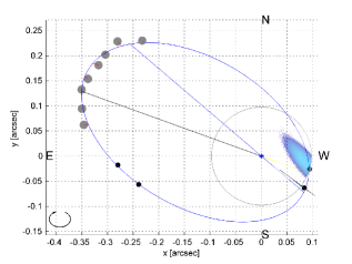
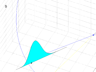
Figure 3: Orbit estimate in presence of incomplete information from our synthetic data on Table 1. The left panel shows the original measurements (grey dots lower weight, black dots higher weight, the two black dots near periastron are only included for reference purposes, but are not part of the solution with imputed values), the maximum likelihood estimate of the orbit (blue line) incorporating the incomplete data at epochs 1944.0 and 1945.0, and the zones were missing observations may fall (calculated with the proposed imputation method). The right panel is a view in detail of the PDF for the angular separation $\rho$ along the line $\vartheta=217.14^{\circ}$ for the case $\rho\in(0,\infty)$ at epoch 1945.0

4.1 Analysis of results

Figure 4 presents the marginal PDFs of the main orbital parameters ($P$, $T$, $e$, $a$ and total mass) obtained on each setting, and adds a comparison of the three scenarios on the same graph. In order to facilitate a visual comparison, histograms are replaced by kernel-based densities in the lower right panel, although both convey essentially the same information.

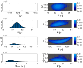
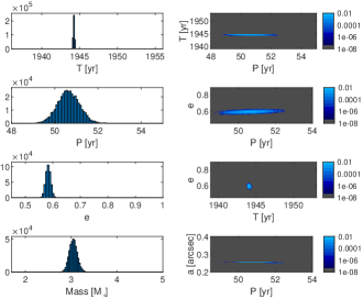
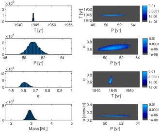
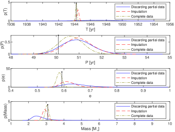
Figure 4: Posterior PDFs of orbital parameters from our synthetic data on Table 1. The four upper left rows show the results obtained when completely discarding the partial observations at epochs 1944.0 and 1945.0 (i.e., the expected result from a standard analysis); the four upper right rows show the results obtained when partial information has been incorporated using our imputation methodology; the four lower left rows show the results obtained using complete information (i.e., as if observations at epochs 1944.0 and 1945.0 had measurements for both $\rho$ and $\vartheta$ as indicated in Table 1, i.e., the best possible case from the available data set). Finally, the four lower right panels compare the marginal PDFs of the three cases on the same figure (the true parameter value is indicated with a black vertical bar).

In a certain sense, the general technique described in Algorithm 1 (being Algorithm 2 an implementation for the specific problem of visual binaries) is based on augmenting the parameter vector with “slots” for the missing measurements, thus estimating both of them simultaneously. The simplest, most evident conclusion of the experiment is that the scheme developed in this paper achieves the objective of sampling both quantities of interest in parallel (i.e., $\theta$ and $\mathcal{Y}_{\textrm{mis}}$), regardless of the quality of the results from an estimation point of view –how the incorporation of additional data affects the estimation is a rather different question. Figure 3 gives a demonstration of the capability of this method to characterize the uncertainty about the missing observations; Figure 4, on the other hand, reveals how the resulting posterior PDFs of orbital parameters differ from each other on each scenario.

As can be seen in Figure 3, this “multiple imputation via MCMC” scheme manages to characterize the feasible values of the partial measurements on the plane of the sky, simultaneously integrating the geometric restrictions of partial measurements and the information about $\theta$ conveyed by complete measurements. It is worth noting that, as values of $\mathcal{Y}_{\textrm{mis}}$ and $\theta$ influence each other along the succession of Imputation and Posterior steps, the final results for both $\mathcal{Y}_{mis}$ and $\theta$ are different from those that would have arisen from each source of knowledge on its own: according to geometric restrictions, feasible values would be evenly distributed within either a circular zone ($\rho\in(0,\rho_{\textrm{max}})$, see left panel of Figure 3) or an infinite line ($\vartheta=\vartheta^{\ast}$, see right panel of Figure 3); according to complete measurements, the location of partial observations would be defined by an a priori set of feasible orbits (which induce “real” positions in the epochs of interest) plus some kind of observational noise. That scheme, however, ignores the influence that imputed observations would exert on the orbital parameters being estimated (in the case of the $\rho\in(0,\rho_{\textrm{max}})$ observation, for example, the support of the resulting PDF covers a much larger area within the circle if compared with that obtained by means of Algorithm 2 and displayed in the left panel of Figure 3).

In Figure 4, the posterior PDFs of the target parameters obtained for each of the scenarios previously described are displayed for comparison purposes. In general, parameter uncertainty decreases as more information is incorporated: of course, the tightest PDFs are obtained in the third scenario (ideal setting with complete information), whereas the widest, least concentrated PDFs are obtained when partial information is discarded (first scenario). Results of the second setting (partial information incorporated via Algorithm 2) lie somewhere in the middle. The lower right panel of Figure 4 is the most explicit graph in this regard, clearly showing the peaks of the PDFs and how concentrated they are. However, not all parameters are equally affected by the incorporation of information (or lack of): while the uncertainties of both $T$ and (very relevant from the astrophysical point of view) the mass sum decrease dramatically with the incorporation of partial data, the marginal PDF of $e$ obtained in the second scenario resembles more that obtained in the first setting than that obtained with complete information; the PDFs obtained for $P$, on the other hand, are quite similar in the three cases. Joint marginal PDFs undergo a similar change: the distribution of $e$ vs. $T$, for example, shows a bow-shaped profile in the first scenario, turning into a convex shape when partial observations are included, and reaching a Gaussian-like form in the complete information scenario.

In summary, the tests performed in this section, aside from presenting a demonstration that the methodology developed throughout actually works as claimed, strongly suggests that the incorporation of partial information into the analysis tools has the clear potential of decreasing the orbital parameter estimation uncertainties.

5 A case study: the visual binary star HU177

In this section, the methodology proposed in Section 3, and tested in Section 4 with synthetic data, is applied to a real object: the visual binary star HU177 (WDS J17305-1446AB = HIP 85679 = HD 158561). This object has been recently studied (using only complete data) by Mendez et al. (2017). The reason for choosing HU177 for a case study is that, among objects with partial data, this is one for which the incorporation of partial measurements may make a relevant difference in terms of the results of the inference. For objects with a well determined orbit, like STF 2729AB (WDS J20514-0538AB = HIP 102945 = HD 198571, grade 2, “good”), for which a large amount of incomplete observations are also available, the incorporation of partial measurements into the analysis would hardly affect the value of the estimated parameters and the uncertainty associated (we have actually verified this by running our imputation code on this data-set). On the other hand, objects with a highly indeterminate orbit (grade 5) are equally inadequate for testing the incorporation of partial measurements, since such a level of uncertainty would induce spatially disperse imputations (compare left and right panels of Figure 5: with less information, the area covered by the support of the PDF of the partial measurement is larger). HU177 has relatively few complete observations (16 in total), distributed unevenly from 1900 to 2015 and showing varying degrees of precision. According to the results obtained when all the 16 complete observations are used to characterize the orbit (third row in Table 4), the orbital parameters of this star are neither tightly constrained nor extremely indeterminate–this is precisely the scenario in which partial measurements may make a contribution. The measurements available for HU177 are given in Table 2, and were kindly provided to us by Dr. William Hartkopf from the US Naval Observatory as part of the WDS effort (it includes 15 complete observations, plus one partial datum at epoch 1991.25 reported by the Hipparcos satellite), supplemented with our own (complete) measurement at epoch 2015.5409 from the SOAR/HRCam Speckle camera reported in Tokovinin et al. (2016), and used by Mendez et al. (2017) to compute an orbit of HU177 (excluding the partial datum).

Table 2: Observations for the visual binary HU177.

Epoch	$\rho$	$\vartheta$	$\sigma_{\rho}$
(yr)	$(^{\prime\prime})$	(∘)	$(^{\prime\prime})$
1900.54	0.370	85.2	0.250
1923.80	0.360	83.9	0.050
1936.61	0.320	67.3	0.050
1938.30	0.340	64.8	0.050
1944.36	0.300	57.2	0.050
1957.62	0.280	33.1	0.050
1958.45	0.220	34.2	0.050
1958.52	0.260	39.8	0.050
1962.59	0.210	28.9	0.050
1989.3121	0.142	275.7	0.005
1991.250	$(0,~{}0.1)$	$(0,~{}360)$	0.015
2007.6013	0.205	199.8	0.015
2008.5397	0.2217	188.5	0.001
2008.5397	0.2234	188.2	0.003
2008.6052	0.223	188.5	0.001
2010.5908	0.228	184.9	0.002
2015.5409	0.2587	176.6	0.002

The test performed in this section comprehends two different data sets: the first is identified by HU177 and contains all the complete measurements available, plus the partial observation; the second one, identified as HU177^∗, contains all the complete measurements except for the one near the periastron (epoch $1989.312$), plus the partial observation (the discarded observation can be noticed in Figure 5). The “assembly” of two separate data sets is carried out in order to better assess the impact of the partial observation: in presence of a complete observation occurring closely in time and space (as in data set HU177), the partial observation may be redundant or even a source of additional uncertainty (recall that Section 2 identifies three sources of uncertainty associated to the imputation process). For each data set, two cases are addressed: without and with multiple imputation. In the first case the partial measurement is omitted completely, then the data set is analyzed by means of the Gibbs sampler used in the previous section (the first and third scenarios described there). The second case is analyzed by means of Algorithm 2. Chains were run with the following parameters: $N_{\textrm{steps}}=10^{7}$ (with a thinning factor of $10$ samples); $\sigma_{\log P}$, $\sigma_{T^{\prime}}$, and $\sigma_{e}$ set to the same values used in Section 4. As done for Section 4, details on prior distributions, chain initialization, burn-in period, convergence diagnostics prior for this experiment are shown in Appendix C. When applying the multiple imputation technique, the proposal distribution used to generate samples of $\mathcal{Y}_{mis}$ is set to $\sigma_{\rho}=0.015^{\prime\prime}$, based on the observational error associated to the imaging device that produced the partial measurement. The criteria to fix that value, as well as the weight assigned to the imputed observations in the likelihood function, are topics of further research, and will not be addressed here.

Figure 5 displays the orbits associated to the maximum likelihood estimates obtained for data sets HU177^∗ and HU177 with the incorporation of the partial data. The complete measurements of relative position, as well as the PDF of the partial observation in each scenario, are shown in the same plane. The maximum likelihood parameter values corresponding to each of these solutions are reported in Table 3. On the other hand, Table 4 reports numerically the results obtained for the four cases analyzed in terms of their quartiles: each row has two lines, the first showing the quartiles of the orbital parameters, and the second line reporting the interquartile range (i.e., the difference between the 75% and 25% percentiles). The interquartile range is used as a means to assess how the uncertainty on the corresponding orbital parameter changes when partial information is incorporated.

5.1 Results and analysis

From Figure 5 and Table 3 it is observed that, although similar at first sight, orbit estimates for HU177^∗ and HU177 (both with multiple imputation) have considerable, although not large, differences (see, for example, period $P$). The estimates of angular elements $\omega$ and $\Omega$ exhibit a large numerical difference between both scenarios, but are geometrically close due to the circular nature of angular quantities (see Appendix A.2)–in fact, both the line of nodes and the line that connects periastron and apastron share similar orientation and location in the two orbits. More noticeable is the difference between the PDF of the partial measurement obtained in each case: for HU177^∗, it comprehends almost half the circle defined by $\rho\in(0,\rho_{\textrm{max}})$ (although zones with higher probability are concentrated towards the “western” border) while for HU177, the PDF of the partial measurement is confined to a relatively smaller area.

Despite the larger uncertainty about the partial observation in the case of HU177^∗, the incorporation of partial information has a larger impact on the estimation in the HU177^∗ than in the HU177 data set: in the first setting, the interquartile range of most parameters undergo a dramatic reduction once the multiple imputation scheme is adopted (Table 4, first two rows), whereas in the second setting there is no statistically significant evidence that the partial observation translates into additional knowledge of the system (Table 4, last two rows). Since in HU177^∗ the partial measurement is the only source of information about that particular zone of the orbit (the vicinity of the periastron), it contributes to reducing the uncertainty about orbital parameters significantly. In HU177, on the contrary, that information is redundant –it is the observation dropped in HU177^∗ that contributes to characterize that sector of the orbit. Furthermore, as the imputation process in itself has some uncertainty associated (the three sources described in Section 2), the multiple imputation may add uncertainty to the estimation instead of reducing it in certain cases. That is what apparently happens in the estimation of the total mass of HU177^∗, for example, where the mass sum is more constrained when no imputations are used (Figure 6, fourth row of the left panel). A question stems from the latter observation: if the interquartile range of both $P$ and $a$ decrease when the multiple imputation scheme is adopted, why (and how) the uncertainty of a derived quantity such as the mass sum increases? The explanation might be found in the fact that interquartile range is a rather naïve tool to measure uncertainty, since it basically ignores the shape of the PDFs (aspects such as heaviness of tails, symmetry, etc.). Thus, assessing uncertainty by means of more sophisticated criteria, such as information-theoretic indicators, appears as the next step in this research line. Furthermore, even though the resulting PDF of the mass sum is less concentrated, the multiple imputation estimate obtained for that quantity ($4.17~{}M_{\odot}$) is closer to the mass estimates obtained when no measurement is discarded ($4.42~{}M_{\odot}$); from that point of view, the estimation using imputation improves in terms of accuracy, even though it may not always necessarily improves in terms of precision.

Finally, it is worth mentioning that defining more restrictive feasible areas for missing observations (instead of mere circles and lines) would be of great help to the estimation –the more constricted they are, the more they resemble a well-resolved, point-like observation. In other words, it might be beneficial, from the point of view of parameter estimation and uncertainty characterization, to save as much information as possible when resolving relative position values from interferometric measurements; that means that, if complete resolution is not feasible, an effort could be made by the observers to confine the plausible values to, for example, an angular section instead of a circle centered at the primary star.

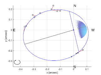
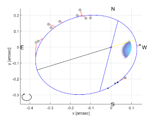
Figure 5: Comparison: visualization of the maximum likelihood orbit estimates for HU177^∗ (left, with the observation near periastron –epoch $1989.312$– discarded) and HU177 (right), both using imputation. The dots indicate the complete observations, larger (grey) dots imply larger uncertainties (lower weight) than black dots (see Table 2). The lighter blue density contours indicate areas of higher probability for the imputed value of $\rho$ at epoch 1991.25. The line of nodes is indicated in blue while the line that connects periastron and apastron are yellow and black respectively (see color version of the figure in the electronic version).

Table 3: Maximum likelihood orbit estimates for HU177 using incomplete information through imputation.

Data set	$P$	$T$	$e$	$a$	$\omega$	$\Omega$	$i$	Mass${}_{\mbox{\tiny{T}}}$
	$(yr)$	$(yr)$		′′	$(^{\circ})$	$(^{\circ})$	$(^{\circ})$	$(M_{\odot})$
HU177∗	$222$	$1987.1$	$0.575$	$0.296$	$81.6$	$10.5$	$147.8$	$4.02$
HU177	$205$	$1986.6$	$0.512$	$0.287$	$240.2$	$168.3$	$151.4$	$4.37$

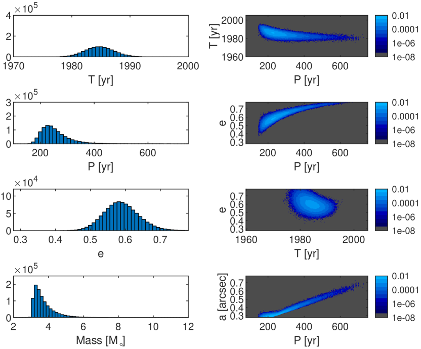
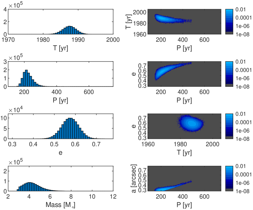
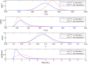
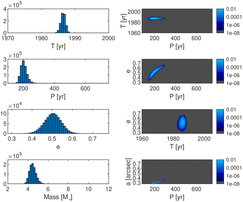
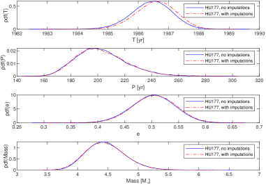
Figure 6: PDFs of orbital parameters of the four cases reported in Table 4. The left columns are for the HU177^∗ data set, the right columns for the HU177 data set. This first four rows show the results for the case of no multiple imputation, while the fifth to eight rows are the results when using multiple imputation. The lower four panels show a comparison between the marginal PDFs for a selected subset of the orbital parameters, and the mass sum (last row).

Table 4: Estimation of orbital parameters for HU177 (based on quartiles of the PDFs) in the presence of incomplete information.

Data set	Use of multiple	$P$	$T$	$e$	$a$	$\omega$	$\Omega$	$i$	Mass${}_{\mbox{\tiny{T}}}$
	imputation	$(yr)$	$(yr)$		′′	$(^{\circ})$	$(^{\circ})$	$(^{\circ})$	$(M_{\odot})$a
HU177∗	No MI	$243.1_{+25.0}^{-34.0}$	$1984.7_{-1.6}^{+1.7}$	$0.587_{-0.032}^{+0.034}$	$0.300_{-0.013}^{+0.021}$	$150.0_{-66.8}^{+27.5}$	$83.9_{-72.5}^{+28.0}$	$154.5_{-6.6}^{+6.1}$	$3.54_{-0.24}^{+0.41}$
		$59.0$	$3.3$	$0.066$	$0.034$	$94.3$	$100.5$	$12.7$	$0.65$
HU177∗	MI	$218.7_{+16.6}^{-21.6}$	$1987.5_{-1.3}^{+1.2}$	$0.575_{-0.027}^{+0.027}$	$0.298_{-0.009}^{+0.011}$	$84.7_{-4.2}^{+4.0}$	$11.9_{-3.7}^{+4.7}$	$145.4_{-5.0}^{+6.1}$	$4.20_{-0.50}^{+0.57}$
		$38.2$	$2.5$	$0.054$	$0.020$	$8.2$	$8.4$	$11.0$	$1.07$
HU177	No MI	$201.2_{+11.7}^{-13.3}$	$1986.5_{-0.5}^{+0.4}$	$0.503_{-0.027}^{+0.027}$	$0.286_{-0.007}^{+0.008}$	$237.5_{-6.5}^{+5.6}$	$165.8_{-5.1}^{+4.4}$	$150.9_{-2.8}^{+3.0}$	$4.45_{-0.20}^{+0.22}$
		$25.0$	$0.9$	$0.054$	$0.016$	$12.1$	$9.6$	$5.8$	$0.43$
HU177	MI	$201.2_{+11.8}^{-13.8}$	$1986.6_{-0.5}^{+0.4}$	$0.505_{-0.027}^{+0.027}$	$0.286_{-0.007}^{+0.009}$	$239.7_{-6.4}^{+5.4}$	$167.9_{-5.0}^{+4.2}$	$150.2_{-2.7}^{+3.0}$	$4.44_{-0.21}^{+0.23}$
		$25.5$	$0.9$	$0.055$	$0.016$	$11.8$	$9.2$	$5.7$	$0.44$

6 Conclusions

This work introduces a scheme for coping with partial measurements in a Bayesian MCMC-based framework for the characterization of visual binary star orbits. The scheme, based on filling missing or partial measurements with a set of plausible values–the so-called multiple imputation approach–, is tested with both synthetic and real measurements of visual binaries. Our results in both scenarios suggest that incorporation of partial measurements can lead to a significant decrease in the uncertainty of the estimation of orbital parameters, although there are also cases where partial measurements provide negligible additional information about the orbit (that is, posterior PDFs undergoing imperceptible changes after the incorporation of partial data). Potentially, multiple imputation could even worsen the quality of estimation, since the process of imputing values also introduces some degree of uncertainty. Those concerns suggest that the assessment of the quality of estimation by means of more sophisticated criteria, such as the comparison of PDFs using information-theoretic tools, should be an important part of future work in this resaerch line.

Partial astrometric measurements intrinsically have a degree of spatial dispersion; however, the tests performed suggest that an interesting improvement in the estimation might arise from restricting their geometric boundaries during the process of reducing and reporting astrometric data, thus feeding estimation routines as the one presented in this work with more constrained boundaries for the unresolved observations than those typically provided.

Appendix A On Thiele-Innes and Campbell elements

A.1 Least-squares estimate

Consider the weighted sum of individual squared errors:

 

$$\sum_{k=1}^{N_{x}}\frac{1}{\sigma_{x}^{2}(k)}[X(k)-X^{\textrm{model}}(k)]^{2}+\sum_{k=1}^{N_{y}}\frac{1}{\sigma_{y}^{2}(k)}[Y(k)-Y^{\textrm{model}}(k)]^{2}$$ (A1)

Equation 10 enables us to replace $X_{\textrm{model}}$, $Y_{\textrm{model}}$ with their analytic expression for any epoch (indexed by $k$), namely:

$$X_{\textrm{obs}}(k)-X_{\textrm{model}}(k) =X_{\textrm{obs}}(k)-[B\cdot x(k)+G\cdot y(k)]$$ (A2)

$$Y_{\textrm{obs}}(k)-Y_{\textrm{model}}(k) =Y_{\textrm{obs}}(k)-[A\cdot x(k)+F\cdot y(k)].$$

Due to the linear dependency of $X_{\textrm{model}}$, $Y_{\textrm{model}}$ with respect to the normalized coordinates $x$, $y$, it is possible to calculate the least-squares estimate for the unknown variables $B$, $G$, $A$, and $F$ in a non-iterative way. Moreover, the first term of Equation A1 depends only on $(B,G)$, whereas second term depends on $(A,F)$. Therefore, the estimate for $(B,G)$ is obtained by minimizing the first term and the estimate for $(A,F)$ by minimizing the second one. The problem is thus reduced to a pair of uncoupled linear equations. By calculating the derivatives of the expression of the error with respect to each of the Thiele-Innes constants and making the results equal to zero, one can obtain the following formulae (for the sake of briefness, a set of auxiliary terms is introduced first):

$$\alpha=\sum_{i}~{}w_{i}~{}x(i)^{2}~{}~{}~{} \beta=\sum_{i}~{}w_{i}~{}y(i)^{2}~{}~{}~{} \gamma=\sum_{i}~{}w_{i}~{}x(i)~{}y(i)$$

$$r_{11}=\sum_{i}~{}w_{i}~{}X_{\textrm{obs}}(i)~{}x(i)~{}~{}~{} r_{12}=\sum_{i}~{}w_{i}~{}X_{\textrm{obs}}(i)~{}y(i)$$

$$r_{21}=\sum_{i}~{}w_{i}~{}Y_{\textrm{obs}}(i)~{}x(i)~{}~{}~{} r_{22}=\sum_{i}~{}w_{i}~{}Y_{\textrm{obs}}(i)~{}y(i)$$ (A3)

Then, the least-squares estimate for the Thiele-Innes constant is calculated as follows:

$$\hat{B}=\frac{\beta\cdot r_{11}-\gamma\cdot r_{12}}{\Delta},~{}~{}~{}~{}~{}~{} \hat{G}=\displaystyle\frac{\alpha\cdot r_{12}-\gamma\cdot r_{11}}{\Delta},$$

$$\hat{A}=\frac{\beta\cdot r_{21}-\gamma\cdot r_{22}}{\Delta},~{}~{}~{}~{}~{}~{} \displaystyle\hat{F}=\frac{\alpha\cdot r_{22}-\gamma\cdot r_{21}}{\Delta},$$

where $\Delta=\alpha\cdot\beta-\gamma^{2}$. An alternative matrix representation is given as follows:

$$\begin{bmatrix}\hat{B}\\ \hat{G}\\ \hat{A}\\ \hat{F}\end{bmatrix}^{T}=[\vec{X}_{\textrm{obs}}\vec{Y}_{\textrm{obs}}]~{}\mathbf{W}\mathbf{F}^{T}(\mathbf{F}\mathbf{W}\mathbf{F}^{T})^{-1}\text{, where }$$ (A4)

$$\mathbf{F}=\begin{bmatrix}x(1)&\dots&x(N)&0&\dots&0\\ y(1)&\dots&y(N)&0&\dots&0\\ 0&\dots&0&x(1)&\dots&x(N)\\ 0&\dots&0&y(1)&\dots&y(N)\end{bmatrix},$$ (A5)

where $\{x(k),y(k)\}_{k=1,\dots,N}$ are the normalized coordinates given $P$, $T$, $e$ and epochs $\{\tau_{k}\}_{k=1,\dots,N}$. $\mathbf{W}$ is a diagonal matrix containing the weight of each observation (usually the reciprocal of the observational error variance).

A.2 Conversion from Thiele-Innes to Campbell

Once the estimates for Thiele-Innes constants are obtained ($\hat{B}$, $\hat{G}$, $\hat{A}$, $\hat{F}$), it is necessary to recover the equivalent Campbell elements representation ($a,\omega,\Omega,i$). For $\omega$ and $\Omega$, one must solve the following equations:

$$\omega+\Omega =\arctan\left(\frac{B-F}{A+G}\right),$$

$$\omega-\Omega =\arctan\left(\frac{-B-F}{A-G}\right),$$

choosing the solution that satisfies that $\sin\left(\omega+\Omega\right)$ has the same sign as $B-F$, and that $\sin\left(\omega-\Omega\right)$ has the same sign as $-B-F$. If that procedure outputs a value of $\Omega$ that does not satisfy the convention that $\Omega\in(0,\pi)$, it must be corrected in the following way: if $\Omega<0$, the values of $\omega$ and $\Omega$ are modified as $\omega=\pi+\omega$, $\Omega=\pi+\Omega$; whereas if $\Omega>\pi$, the values of $\omega$ and $\Omega$ are modified such that $\omega=\omega-\pi$, $\Omega=\Omega-\pi$.

For the semi-major axis $a$ and inclination $i$, the following auxiliary variables must be calculated first:

$$k =\frac{A^{2}+B^{2}+F^{2}+G^{2}}{2},$$

$$m =A\cdot G-B\cdot F,$$

$$j =\sqrt{k^{2}-m^{2}}.$$

Then, $a$ and $i$ are determined with the following formulae:

$$a =\sqrt{j+k}$$

$$i =\arccos\left(\frac{m}{a^{2}}\right)$$

Appendix B Supporting pseudo-code

This section outlines the fundamentals of the MCMC algorithms used in this work. Term $x$ is the variable of interested in (e.g., a parameter vector, the state vector of a system, etc.), $\pi(x)$ represents the target PDF and $q(x^{\prime}|x)$ is a proposal distribution (a distribution to generate new samples of the Markov chain).

Figure 7: Metropolis-Hastings algorithm

Figure 8: Gibbs sampler

Figure 9: Metropolis-Hastings-within-Gibbs

Appendix C Initial state of the Markov chains and convergence diagnostics

To assess whether the algorithm has reached a stationary regime, the convergence criterion introduced in Gelman & Rubin (1992) was used. The so-called Gelman–Rubin R statistic is a tool to evaluate convergence by comparing multiple independent Markov chains. To apply the Gelman–Rubin R statistic, several chains are run, each of them starting from a different point in the parameter space. Then, after calculating quantities $B$ (inter-chain variance, Equation C1) and $W$ (intra-chain variance, Equation C2), $R$ statistic is computed as in Equation C3.

$$B=\displaystyle\frac{N_{\textrm{steps}}}{N_{\textrm{chains}}-1}\sum_{j=1}^{N_{\textrm{chains}}}(\hat{\theta}_{j}-\hat{\theta})^{2}.$$ (C1)

$$W=\displaystyle\frac{1}{N_{\textrm{chains}}}\sum_{j=1}^{N_{\textrm{chains}}}\hat{\sigma}_{j}^{2}.$$ (C2)

$$R=1+\displaystyle\frac{1}{N_{\textrm{steps}}}\cdot\biggl{(}\frac{B}{W}-1\biggr{)}.$$ (C3)

In equations C1, C2, C3, $\theta$ denotes one of the parameters being estimated (i.e., a scalar component of the parameter vector), with $\hat{\theta}$ the average value calculated over all the chains and $\hat{\theta}_{j}$ the average of a single chain. The basic assumption of the R statistic is that, since theory states that all chains have the same stationary distribution, if all runs show a similar behaviour then all of them have reached the stationary regime. In the statistical literature, $R$ values less than $1.05$ are considered an indicator that the algorithm has converged.

C.1 Synthetic data

The algorithm to incorporate partial measurements relies on a good initialization of the parameters $P$, $T^{\prime}$ and $e$ (otherwise, the values of $\mathcal{Y}_{\textrm{mis}}$ in the imputation step may be nonsensical). To ensure that the chain starts from a feasible orbital configuration, each time we run the multiple imputation via MCMC algorithm, we draw its initial state from a preliminary chain run on the sub-set of complete measurements (rather than sampling directly from a non-informative prior). According to our results, the multiple imputation via MCMC algorithm tends to exhibit a behavior that falls between the two scenarios tested: it tends to generate parameter distributions that are are more concentrated than the ones obtained using no partial observations, but more disperse than those obtained when all complete measurements are available. On these grounds, and in order to avoid the computational burden of running several chains of the multiple imputation via MCMC algorithm, no test was performed for this algorithm.

Before running the long chain used to make the inference, we ran ten chains ($10^{6}$ samples long each) to assess convergence via the Gelman–Rubin R statistic. Using the Gaussian proposal distributions indicated in Section 4 and drawing initial values from $p_{\textrm{prior}}(T^{\prime})=\mathbb{1}_{[0,1)}$, $p_{\textrm{prior}}(\log P)=\mathbb{1}_{[10,120)}$, $p_{\textrm{prior}}(e)=\mathbb{1}_{[0,0.99)}$, the test was performed on two different data sets: the sub-set of complete measurements, and the ground-truth setting where all measurements are known. The results are presented in Table 5, where it can be seen that the $R$ statistic is less than $1.05$ for all parameters, indicating that the chains converge (with the parameters specified in this work).

C.2 Real data

The test used for synthetic observations was repeated for the case of real data, with the following priors: $p_{\textrm{prior}}(T^{\prime})=\mathbb{1}_{[0,1)}$, $p_{\textrm{prior}}(\log P)=\mathbb{1}_{[50,1200)}$, $p_{\textrm{prior}}(e)=\mathbb{1}_{[0,0.99)}$. The regular Gibbs sampler was applied on data sets HU177 and HU177^∗ and no test for the multiple imputation via MCMC algorithm was performed. Results are shown in Table 6). The resultant $R$ statistic values were less than $1.05$ for all parameters, indicating that the chains converge.

C.3 Burn-in period

For both synthetic and real data, the burn-in period was set $10^{5}$ samples based on visual inspection of the test chains (i.e., those used to calculate the R statistic plus some other individual trials). In most cases fewer samples were necessary to reach the stationary distribution, but the conservative value $10^{5}$ was chosen thinking of a worst case scenario. These samples are removed from the raw, not the thinned chain.

Table 5: Gelman–Rubin R statistic for experiments with synthetic data

Data set	$P$	$T$	$e$
Complete measurements sub-set	1.0139	1.0026	1.0013
Ground-truth setting	1.0024	1.0024	1.0004

Table 6: Gelman–Rubin R statistic for experiments with real data

Data set	$P$	$T$	$e$
HU177∗	1.0199	1.0192	1.0167
HU177	1.0332	1.0112	1.0119

References

- Andrieu et al. (2003) Andrieu, C., De Freitas, N., Doucet, A., & Jordan, M. I. 2003, Machine learning, 50, 5
- Andrieu et al. (2001) Andrieu, C., Doucet, A., & Punskaya, E. 2001, in Sequential Monte Carlo Methods in Practice (Springer), 79–95
- Brooks et al. (2011) Brooks, S., Gelman, A., Jones, G., & Meng, X.-L. 2011, Handbook of markov chain monte carlo (CRC press)
- Burgasser et al. (2015) Burgasser, A. J., Melis, C., Todd, J., et al. 2015, The Astronomical Journal, 150, 180
- Chattopadhyay & Chattopadhyay (2014) Chattopadhyay, A. K., & Chattopadhyay, T. 2014, Statistical methods for astronomical data analysis, Vol. 3 (Springer)
- Dempster et al. (1977) Dempster, A. P., Laird, N. M., & Rubin, D. B. 1977, Journal of the royal statistical society. Series B (methodological), 1
- Docobo (1985) Docobo, J. 1985, Celestial mechanics, 36, 143
- Evans et al. (1986) Evans, D. S., McWilliam, A., Sandmann, W. H., & Frueh, M. 1986, The Astronomical Journal, 92, 1210
- Ford (2005) Ford, E. B. 2005, The Astronomical Journal, 129, 1706
- Gautier III et al. (2012) Gautier III, T. N., Charbonneau, D., Rowe, J. F., et al. 2012, The Astrophysical Journal, 749, 15
- Gelman et al. (2003) Gelman, A., Carlin, J. B., Stern, H. S., & Rubin, D. B. 2003, Bayesian Data Analysis (Chapman and Hall/CRC)
- Gelman & Rubin (1992) Gelman, A., & Rubin, D. B. 1992, Statistical science, 457
- Gelman et al. (2013) Gelman, A., Stern, H. S., Carlin, J. B., et al. 2013, Bayesian data analysis (Chapman and Hall/CRC)
- Gelman et al. (2006) Gelman, A., et al. 2006, Bayesian analysis, 1, 515
- Geman & Geman (1984) Geman, S., & Geman, D. 1984, IEEE Transactions on pattern analysis and machine intelligence, 6, 721
- Gillon et al. (2017) Gillon, M., Triaud, A. H., Demory, B.-O., et al. 2017, Nature, 542, 456
- Gregory (2005) Gregory, P. 2005, The Astrophysical Journal, 631, 1198
- Hartkopf et al. (1989) Hartkopf, W. I., McAlister, H. A., & Franz, O. G. 1989, The Astronomical Journal, 98, 1014
- Hartkopf et al. (2001) Hartkopf, W. I., McAlister, H. A., & Mason, B. D. 2001, AJ, 122, 3480, doi: 10.1086/323923
- Hastings (1970) Hastings, W. K. 1970, Biometrika, 57, 97
- Lavori et al. (1995) Lavori, P. W., Dawson, R., & Shera, D. 1995, Statistics in medicine, 14, 1913
- Little & Rubin (2002) Little, R. J., & Rubin, D. B. 2002, Statistical analysis with missing data, Vol. 793 (Wiley)
- Lucy (2014) Lucy, L. 2014, Astronomy & Astrophysics, 563, A126
- Mason et al. (2001) Mason, B. D., Wycoff, G. L., Hartkopf, W. I., Douglass, G. G., & Worley, C. E. 2001, The Astronomical Journal, 122, 3466
- Mendez et al. (2017) Mendez, R. A., Claveria, R. M., Orchard, M. E., & Silva, J. F. 2017, AJ, 154, 187, doi: 10.3847/1538-3881/aa8d6f
- Metropolis et al. (1953) Metropolis, N., Rosenbluth, A. W., Rosenbluth, M. N., Teller, A. H., & Teller, E. 1953, The journal of chemical physics, 21, 1087
- Metropolis & Ulam (1949) Metropolis, N., & Ulam, S. 1949, Journal of the American statistical association, 44, 335
- Pourbaix (1994) Pourbaix, D. 1994, Astronomy and Astrophysics, 290, 682
- Rowe et al. (2014) Rowe, J. F., Bryson, S. T., Marcy, G. W., et al. 2014, The Astrophysical Journal, 784, 45
- Rubin (1987) Rubin, D. 1987, Multiple Imputation for Nonresponse in Surveys (Wiley)
- Rubin (1976) Rubin, D. B. 1976, Biometrika, 581
- Sahlmann et al. (2013) Sahlmann, J., Lazorenko, P., Ségransan, D., et al. 2013, Astronomy & Astrophysics, 556, A133
- Spiegelhalter et al. (1996) Spiegelhalter, D., Thomas, A., Best, N., & Gilks, W. 1996, MRC Biostatistics Unit, Institute of Public Health, Cambridge, UK, 1
- Tanner & Wong (1987) Tanner, M. A., & Wong, W. H. 1987, Journal of the American statistical Association, 82, 528
- Thiele (1883) Thiele, T. N. 1883, Astronomische Nachrichten, 104, 245
- Tierney (1994) Tierney, L. 1994, The Annals of Statistics, 1701
- Tokovinin (2018) Tokovinin, A. 2018, PASP, 130, 035002, doi: 10.1088/1538-3873/aaa7d9
- Tokovinin et al. (2016) Tokovinin, A., Mason, B. D., Hartkopf, W. I., Mendez, R. A., & Horch, E. P. 2016, AJ, 151, 153, doi: 10.3847/0004-6256/151/6/153
- Van de Kamp & Stearns (1967) Van de Kamp, P., & Stearns, C. L. 1967, American Journal of Physics, 35, 974
- Yuan (2010) Yuan, Y. C. 2010, SAS Institute Inc, Rockville, MD, 49, 1
- Zhang (2003) Zhang, P. 2003, International Statistical Review, 71, 581