Effect of Strain on Charge Density Wave Order in the Holstein Model

Abstract

We investigate charge ordering in the Holstein model in the presence of anisotropic hopping, $t_{x},t_{y}=1-\delta,1+\delta$, as a model of the effect of strain on charge density wave (CDW) materials. Using Quantum Monte Carlo simulations, we show that the CDW transition temperature is relatively insensitive to moderate anisotropy $\delta\lesssim 0.3$, but begins to decrease more rapidly at $\delta\gtrsim 0.4$. However, the density correlations, as well as the kinetic energies parallel and perpendicular to the compressional axis, change significantly for moderate $\delta$. Accompanying mean-field theory calculations show a similar qualitative structure, with the transition temperature relatively constant at small $\delta$ and a more rapid decrease for larger strains. We also obtain the density of states $N(\omega)$, which provides clear signal of the charge ordering transition at large strain, where finite size scaling of the charge structure factor is extremely difficult because of the small value of the order parameter.

I Introduction

Studies of the effect of strain in charge density wave (CDW) materials have seen a significant rise in the past several years Gan et al. (2016); Wei et al. (2017); Gao et al. (2018). The general interest originates from the ability to tune a strongly correlated insulating phase, inducing transitions into alternate patterns of charge order, or into metallic and even superconducting phases. Moreover, by altering the band structure, the application of strain also provides specific insight into the nature of a native CDW phase, for instance into the role of Fermi surface nesting Johannes et al. (2006); Johannes and Mazin (2008). Layered transition metal dichalcogenides (TMDs) are one of the most commonly investigated classes of CDW materials; their transitions have previously been tuned by varying the thickness or gate potential Tsen et al. (2015); Yang et al. (2014); Renteria et al. (2014); Yu et al. (2015); Hollander et al. (2015); Samnakay et al. (2015). In 2$H$-NbSe₂ the CDW transition temperature $T_{\rm cdw}$ increases from $T_{\rm cdw}=33$ K in the bulk to $T_{\rm cdw}=145$ K in a single layer Xi et al. (2015). A similar, albeit much smaller, effect is seen in 1$T$-TiSe₂ Chen et al. (2015, 2016). Strain is therefore useful since it provides an alternate method for modulating CDW physics. Indeed, exploration of the potential use of strain to adjust optical, magnetic and conductive properties, especially in TMDs, has been referred to as ‘strain engineering’.

Much of the existing theoretical work in the area has been within first-principles density functional theory (DFT). These studies find that for 1$T$-TiSe₂ the CDW transition temperature can be enhanced or suppressed with the application of tensile or compressive strain, respectively Wei et al. (2017). In the latter case, the weakened CDW opens the door for superconductivity (SC). This difference in effect is linked to the distinct behavior of the band gap upon extension versus compression. For thin layers of TMDs, the intercalation of chemical compounds between layers, such as Na-intercalated NbSe₂, leads to strain, which has been shown to enhance SC Lian et al. (2017). Initially, the Na intercalation creates a large electron doping, which contracts the Fermi surface and causes CDW to disappear. The subsequent application of strain increases the density of states at the Fermi surface and more than doubles the SC transition temperature.

CDW materials, including the TMDs, generally have complex (e.g. layered) structures. The charge ordering may not be commensurate with the lattice, and may also differ on the surface and within the bulk. The application of strain has additional complicating effects, including changes in the phonon spectrum and of the relative placement of different orbitals (energy bands). In particular, 1$T$-VSe₂ has a transition from hexagonal to rectangular charge order with strain, which seems to originate in the softening of certain phonon modes Zhang et al. (2017). The aforementioned DFT investigations have explored many of these details.

An alternate theoretical approach to DFT which lends complementary insight into CDW physics is through the solution of simple lattice Hamiltonians. One set of models focuses on intersite electron-electron interactions $V$, as described, for example, by the extended Hubbard Hamiltonian Sengupta et al. (2002); Hirsch (1985); Iglovikov et al. (2015). Here, charge order arises directly from the minimization of the intersite repulsion energy $V$ by alternating empty and occupied sites. A more realistic approach for TMDs, however, would be including electron-phonon interactions, such as those incorporated in the Holstein Holstein (1959) or Su-Schrieffer-Heeger Su et al. (1979) models. In these cases, the driving force for CDW formation is a lowering of the electron kinetic energy through the opening of a gap in the spectrum. This energy lowering competes with the cost in elastic energy associated with phonon displacements.

CDW formation on surfaces and in quasi-2D materials have been motivating theoretical studies of the Holstein model in two dimensions. In addition to the choice of the CDW driving interaction (electron-electron-like or electron-phonon-like), lattice geometry plays an important role in the presence of charge ordering. For instance, for the Holstein model in a honeycomb lattice, one may show that a finite critical electron-phonon coupling is required for CDW Costa et al. (2018); Chen et al. (2019), while in the triangular lattice its ground state exhibits SC Li et al. (2018).

In view of these simulation results, here we investigate how charge-charge correlations are affected by deformations in the lattice, that is, we focus on the effects of strain on charge ordering. To this end, we investigate the Holstein model on a square lattice using determinant quantum Monte Carlo (DQMC) simulations, and incorporate the most direct effect of strain, the enhancement of the orbital overlap integral by compression, through an anisotropy in the hopping in the $x$ and $y$ directions. We find that although $T_{\rm cdw}$ is relatively insensitive to anisotropy $\delta\lesssim 0.3$, the density correlations and kinetic energy change significantly even at small strain. It is only at larger anistropy $\delta\gtrsim 0.4$ that significant changes in $T_{\rm cdw}$ are observed. The paper is organized as follows: in Sec. II we present the main features of the Holstein Hamiltonian, defining the parameters of interest; Sec. III describes and presents results for a mean-field approach, while DQMC results are presented in Sec. IV; in Sec. V we discuss the results and summarize our main conclusions.

II The Model

The Holstein Hamiltonian, which describes electrons interacting locally with ions, is given by

$$\mathcal{\hat{H}}= -t_{x}\sum_{\mathbf{i},\sigma}\big{(}\,\hat{d}^{\dagger}_{\mathbf{i},\sigma}\hat{d}^{\phantom{\dagger}}_{\mathbf{i}+\hat{x},\sigma}+\hat{d}^{\dagger}_{\mathbf{i}+\hat{x},\sigma}\hat{d}^{\phantom{\dagger}}_{\mathbf{i},\sigma}\,\big{)}$$

$$-t_{y}\sum_{\mathbf{i},\sigma}\big{(}\,\hat{d}^{\dagger}_{\mathbf{i},\sigma}\hat{d}^{\phantom{\dagger}}_{\mathbf{i}+\hat{y},\sigma}+\hat{d}^{\dagger}_{\mathbf{i}+\hat{y},\sigma}\hat{d}^{\phantom{\dagger}}_{\mathbf{i},\sigma}\,\big{)}-\mu\sum_{\mathbf{i},\sigma}\hat{n}_{\mathbf{i},\sigma}$$

$$+\frac{1}{2}\sum_{\mathbf{i}}\hat{P}^{2}_{\mathbf{i}}+\frac{\omega_{\,0}^{2}}{2}\sum_{\mathbf{i}}\hat{X}^{2}_{\mathbf{i}}+\lambda\sum_{\mathbf{i},\sigma}\hat{n}_{\mathbf{i},\sigma}\hat{X}_{\mathbf{i}}\,\,.$$ (1)

Here $\hat{d}^{\dagger}_{\mathbf{i},\sigma}(\hat{d}_{\mathbf{i},\sigma})$ are creation (destruction) operators for a fermion of spin $\sigma=\uparrow,\downarrow$ at site $\mathbf{i}$ of a two-dimensional square lattice. Thus, the first term represents an electron kinetic energy (band structure) with hoppings $t_{x},t_{y}$ and dispersion $\epsilon_{\bf k}=-2t_{x}\,{\rm cos}\,k_{x}-2t_{y}\,{\rm cos}\,k_{y}$. $\hat{P}_{\mathbf{i}}$ and $\hat{X}_{\mathbf{i}}$ describe a local phonon mode of frequency $\omega_{0}$ on site $\mathbf{i}$, where the phonon mass has been normalized to $M=1$. The electron-phonon coupling $\lambda$, also sometimes reported in terms of $g=\frac{\lambda}{\sqrt{2\omega_{0}}}$, connects the electron density $\hat{n}_{\mathbf{i},\sigma}=\hat{d}^{\dagger}_{\mathbf{i},\sigma}\hat{d}_{\mathbf{i},\sigma}$ for spin $\sigma$ at site $\mathbf{i}$ with the displacement $\hat{X}_{\mathbf{i}}$, where $\mu=-\frac{\lambda^{2}}{\omega_{0}^{2}}$ is the chemical potential at half-filling.

At constant volume, compression along one axis is accompanied by an expansion in the orthogonal direction. Thus, in what follows, we set $t_{x}=t(1-\delta)$ and $t_{y}=t(1+\delta)$, a choice which keeps $t_{x}+t_{y}=2t$, and hence the bandwidth $W=4(t_{x}+t_{y})$ constant. This is motivated physically by the remarks above, but also allows us to separate the effect of hopping anisotropy from changes which would accompany a simple isotropic reduction or enhancement of $W$.

The electron-phonon interaction promotes local pairing of electrons. This can easily be seen by considering the single site ($t=0$) limit. Integrating out the phonon degrees of freedom leads to an effective attraction between the up and down spin fermions $U_{\rm eff}\,n_{\mathbf{i},\uparrow}n_{\mathbf{i},\downarrow}$, with $U_{\rm eff}=-\lambda^{2}/\omega_{0}^{2}$. Associated with this attraction is an oscillator displacement $\langle X\rangle=-\lambda\langle n\rangle/\omega_{0}^{2}$ where $\langle n\rangle=\langle n_{\uparrow}+n_{\downarrow}\rangle$ is the density.

At strong coupling, local pairs form due to this on-site attraction. These pairs prefer to organize their placements spatially. In particular, as the density approaches half-filling, $\langle n\rangle=1$, on a bipartite lattice, electron pairs and empty sites alternate on the two sublattices. This CDW pattern is favored because the energy of neighboring occupied and empty sites is lower by $4t^{2}/U_{\rm eff}$ relative to two adjacent occupied or empty sites. This argument closely parallels the one which motivates the appearance of antiferromagnetic (AF) order in the large $U$ (Heisenberg) limit of the half-filled repulsive Hubbard model, where well-formed local moments of up and down spin alternate due to the $J\sim 4t^{2}/U$ lowering of the energy relative to parallel spin placement.

There is a further analogy between the Hubbard and Holstein Hamiltonians at weak coupling. In the Hubbard model at $U\lesssim W$, AF order is associated with Fermi surface nesting and a ‘Slater insulating’ phase – the opening of an AF gap lowers the electron kinetic energy. Meanwhile, for $U\gtrsim W$ one has a Mott insulator in which AF order arises via $J$. In the Holstein model, an alternation of phonon displacements opens a CDW gap, with similar effect. It is interesting that these close analogies exist, in the weak coupling limit, despite the fact that the Holstein Hamiltonian has a second set of (phonon) degrees of freedom which is absent in the Hubbard Hamiltonian. Although the Holstein model has no strong coupling Mott phase, one still expects the CDW ordering temperature $T_{\rm cdw}$ to decline at large $U_{\rm eff}$ (large $\lambda$). This expectation is not realized within the analytic Eliashberg treatment, but has been observed in quantum Monte Carlo (QMC) simulations Weber and Hohenadler (2018); Zhang et al. (2019).

III Mean-Field Theory

We first solve Eq. (1) by making an adiabatic approximation in neglecting the phonon kinetic energy, and then apply a simple mean-field ansatz by letting $\hat{X}_{\mathbf{i}}\rightarrow x_{0}+(-1)^{\mathbf{i}}\,x_{1}$. The value $x_{0}$ describes a site-independent phonon displacement which is given by $-\frac{\lambda}{\omega_{0}^{2}}$ at half-filling, similar to that described in the preceding section. Meanwhile $x_{1}$ is the CDW order parameter: a nonzero value breaks the symmetry between the two (equivalent) sublattices.

Inserting this form into Eq. (1), the quadratic Hamiltonian can be diagonalized. From the resulting electronic energy levels $E_{\alpha}$ one can compute the free energy as a function of the order parameter $x_{1}$,

$$F=\frac{N}{2}\omega_{0}^{2}(x_{0}^{2}+x_{1}^{2})-T\sum_{\alpha,\sigma}{\rm ln}\big{(}1+e^{-\beta E_{\alpha}(x_{1})}\big{)}$$ (2)

Minimizing $F(x_{1})$ determines the presence ($x_{1}>0$) or absence ($x_{1}=0$) of CDW order. Since the product of the coupling constant $\lambda$ and the phonon displacement $x_{\mathbf{i}}$ provides a staggered chemical potential at site ${\bf i}$, a non-zero value of $x_{1}$ will result in an alternating electron density, that is, CDW order.

An equivalent iterative approach is as follows: given some intial $x_{0}$ and $x_{1}$, the (quadratic) Hamiltonian is diagonalized and the resulting charge densities $n_{\mathbf{i}}=n+(-1)^{\mathbf{i}}\,\Delta n$ are computed. Using these values, $x_{0}$ and $x_{1}$ are updated via $x_{0}=(-\lambda/\omega_{0}^{2})\,n$ and $x_{1}=(\lambda/\omega_{0}^{2})\,\Delta n$. This process is iterated to convergence.

It is evident that within mean-field theory (MFT) the behavior of the Holstein model is governed only by the combination $\lambda^{2}/\omega_{0}^{2}$ rather than on $\lambda$ and $\omega_{0}$ individually. This is also the case at $t=0$, but is only approximately true in exact solutions, e.g. within DQMC. Nevertheless, it is convenient to define the dimensionless coupling constant $\lambda_{D}\equiv\lambda^{2}/(\omega_{0}^{2}\,W)$ where $W=8t$ is the fermion bandwidth, and present results as functions of $\lambda_{D}$.

Figure 1 shows the MFT behavior of $x_{1}$ as function of the inverse temperature for different values of $\delta$, given lattice size of $L=150$. Note that, as expected, there is a finite-temperature second-order phase transition, and that the maximum value that $x_{1}$ approaches at low temperatures changes significantly with $\delta$. This behavior is also reflected in the inset of Fig. 2, showing that the difference in electron density between the two sublattices $\Delta n$ decreases with increasing $\delta$ in the $T\rightarrow 0$ limit. Because of the $x\leftrightarrow y$ symmetry, we expect $T_{\rm cdw}(-\delta)=T_{\rm cdw}(\delta)$, where the change in the critical temperature is a monotonically decreasing even function of $\delta$.

Since the CDW phase transition in the Holstein model is at the same universality class of the 2D Ising model, it is worth comparing our MFT results (and subsequent DQMC results) for $\beta_{c}$ with those from the 2D anisotropic Ising model, i.e. $J_{x}\neq J_{y}$. Within a mean-field approach for $J_{x}=1-\delta$ and $J_{y}=1+\delta$, one obtains $2\beta_{c}(J_{x}+J_{y})=1$, giving $\beta_{c}=1/4$ that is completely independent of $\delta$, in stark contrast to the exact Onsager solution. Unlike the Ising model, the $\beta_{c}$ obtained using a mean-field approach for the CDW transition in the Holstein model depends on $\delta$. This occurs because the density of states at the Fermi surface is modified via the effect of $\delta$ on the band structure.

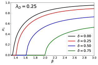
Figure 1: The mean-field order parameter $x_{1}$ versus $\beta$ for four different values of strain $\delta$ at $\lambda_{D}=0.25$. The critical transition temperature $T_{\rm cdw}=\beta_{c}^{-1}$ decreases with increasing strain. See Fig. 2.

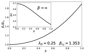
Figure 2: The mean-field critical temperature $\beta_{c}/\beta_{c_{0}}$ versus the strain $\delta$ for $\lambda_{D}=0.25$ where $\beta_{C0}=1.353$ in the isotropic $\delta=0$ case. The inset shows the mean-field result for the difference in electron density between the two sub-lattices $\Delta n$ in the limit that $\beta\rightarrow\infty$.

IV Quantum Monte Carlo

IV.1 Methodology

We next treat the Hamiltonian of Eq. (1) with determinant quantum Monte Carlo method Blankenbecler et al. (1981); Hirsch (1985); White et al. (1989). A detailed discussion of this approach may be found in reviews, such as Refs. Gubernatis et al., 2016; Assaad, 2002; dos Santos, 2003. In evaluating the partition function ${\cal Z}={\rm Tr}\,e^{-\beta\mathcal{\hat{H}}}$, the inverse temperature is discretized into $L_{\tau}$ intervals of length $\beta=L_{\tau}\Delta\tau$. Complete sets of phonon position eigenstates $\{\,|\,x_{\mathbf{i}}(\tau)\,\rangle\,\}$ are then introduced between each incremental imaginary-time evolution operator $e^{-\Delta\tau\mathcal{\hat{H}}}$. The action of the quantum oscillator pieces in the third line of Eq. (1) on $|\,x_{\mathbf{i}}(\tau)\,\rangle\,$ leads to the usual “bosonic’ action,

$$S_{\rm Bose}= \Delta\tau\bigg{[}\,\frac{1}{2}\omega_{0}^{2}\sum_{\mathbf{i,\tau}}x_{\mathbf{i}}(\tau)^{2}$$

$$+\frac{1}{2}\sum_{\mathbf{i,\tau}}\bigg{(}\frac{x_{\mathbf{i}}(\tau+1)-x_{\mathbf{i}}(\tau)}{\Delta\tau}\bigg{)}^{2}\bigg{]}\,.$$ (3)

The fermionic operators appear only quadratically, and can be traced out analytically. The result is the product of the determinants of two matrices $M_{\sigma}(\{x_{\bf i}(\tau)\})$, one for each of spin $\uparrow,\downarrow$. The remaining trace over the phonon field involves a sum over the classical variables $x_{\mathbf{i}}(\tau)$ indexed by the two spatial and one imaginary-time directions, with a weight given by $e^{-S_{\rm Bose}}\,{\rm det}M_{\uparrow}(\{x_{\bf i}(\tau)\}){\rm det}M_{\downarrow}(\{x_{\bf i}(\tau)\})$. This sum is done via a Monte Carlo sampling using both single and global updates.

Because the two spin species couple in the same way to the phonon coordinates, the matrices $M_{\sigma}$ are identical for $\sigma=\uparrow,\downarrow$. Hence the product of their determinants, which enters the weight of the configuration $\{x_{\mathbf{i}}(\tau)\}$, is always positive, ensuring there is no ‘sign problem’ Loh et al. (1990); Troyer and Wiese (2005) at any temperature, density or Hamiltonian parameter values. Nevertheless, in order to emphasize the effects of strain, we limit our analysis to the half-filling case, i.e. $\langle n_{\mathbf{i}\sigma}\rangle=\frac{1}{2}$, where a commensurate CDW phase is known to exist below a given critical temperature Weber and Hohenadler (2018).

The principle limitations of DQMC, as with most Monte Carlo simulations, are finite lattice sizes and statistical error bars on the observables. One way in which finite size errors manifest in DQMC is via the discrete set of momentum points $\{{\bf k}\}$. Here we use antiperiodic boundary conditions for lattices with linear size $L=6$, 10 and 14 and periodic boundary conditions for $L=4$, 8 and 12. This ensures that the four ${\bf k}$ points $(\pm\frac{\pi}{2},\pm\frac{\pi}{2})$ fall directly on the Fermi Surface for all lattice sizes, mitigating otherwise substantial finite size effects.

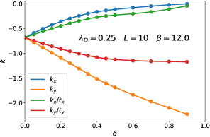
Figure 3: The electron kinetic energies $k_{x}$ and $k_{y}$ are shown as functions of $\delta$. Division by the energy scales $t_{x}$ and $t_{y}$ isolates the effect of anisotropy on the hopping.

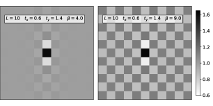
Figure 4: Left Panel: Real space density-density correlations for a moderate strain of $\delta=0.4$ at $T>T_{\rm cdw}$. Note the enhanced correlations in the $\hat{y}$ direction relative to the $\hat{x}$ direction. Right Panel: Real space density-density correlations for $\delta=0.4$ at $T<T_{\rm cdw}$. Note that the oscillating checkerboard charge density pattern now persists across the entire lattice.

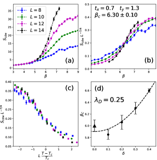
Figure 5: Panel (a): $S_{\rm cdw}$ versus $\beta$ for $\delta=0.3$, $\lambda_{D}=0.25$ and four different lattice size. Panel (b): A finite size scaling where the scaled structure factors $S_{\rm cdw}L^{-\gamma/\nu}$ exhibit a crossing as a function of $\beta$ for different lattice sizes $L$. We infer $\beta_{c}=6.3\pm 0.1$ is slightly increased from the isotropic $\beta_{c}=6.0$. Panel (c): The full data collapse in which the temperature axis is also scaled by $L^{1/\nu}\left(\frac{T-T_{\rm cdw}}{T_{\rm cdw}}\right)$. Panel (d): $\beta_{c}$ as a function of $\delta$. The dashed line is a least squares fit to the data. The value of $\beta_{c}$ at $\delta=0$ (triangle) is from Ref. Costa et al., 2018.

Using DQMC, we are able to access a wide variety of observables, since expectation values of fermionic operators are straightforwardly expressed in terms of matrix elements of $G_{\sigma}=M_{\sigma}^{-1}$ and their products. In what follows, we consider first the kinetic energies in the $x$ and $y$ directions,

$$k_{x} \equiv\big{\langle}\,-t_{x}\sum_{\sigma}\big{(}\,\hat{d}^{\dagger}_{\mathbf{i},\sigma}\hat{d}^{\phantom{\dagger}}_{\mathbf{i}+\hat{x},\sigma}+\hat{d}^{\dagger}_{\mathbf{i}+\hat{x},\sigma}\hat{d}^{\phantom{\dagger}}_{\mathbf{i},\sigma}\,\big{)}\,\big{\rangle}$$

$$k_{y} \equiv\big{\langle}\,-t_{y}\sum_{\sigma}\big{(}\,\hat{d}^{\dagger}_{\mathbf{i},\sigma}\hat{d}^{\phantom{\dagger}}_{\mathbf{i}+\hat{y},\sigma}+\hat{d}^{\dagger}_{\mathbf{i}+\hat{y},\sigma}\hat{d}^{\phantom{\dagger}}_{\mathbf{i},\sigma}\,\big{)}\,\big{\rangle}$$ (4)

and the staggered CDW structure factor

$$S_{\rm cdw} =\frac{1}{N}\sum_{\mathbf{i,r}}(-1)^{\bf r}\big{\langle}\big{(}\,n_{\mathbf{i}\uparrow}+n_{\mathbf{i}\downarrow}\,\big{)}\,\big{(}\,n_{\mathbf{i+r}\uparrow}+n_{\mathbf{i+r}\downarrow}\,\big{)}\big{\rangle}$$

$$=\frac{1}{N}\sum_{\mathbf{i,r}}(-1)^{\bf r}c(\mathbf{r})\,,$$ (5)

which is the Fourier transform at $\mathbf{q}=(\pi,\pi)$ of the real space density correlation functions $c(\mathbf{r})$, and is proportional to the square of the order parameter when extrapolated to the thermodynamic limit. When making these measurements we use $\Delta\tau=0.125$, which is small enough that the Trotter errors associated with the discretization of $\beta$ are smaller than the statistical ones.Scalettar et al. (1991)

IV.2 Equal-Time Correlations

The kinetic energy directly measures the effect of strain via an anisotropic hopping in the $x$ and $y$ directions. We will also display $k_{x}/t_{x}$ and $k_{y}/t_{y}$ to isolate the ‘trivial’ factor of the energy scales. Figure 3 shows the kinetic energies as functions of the hopping anisotropy $\delta$. These evolve smoothly with $\delta$, increasing in the $y$ direction, for which $t_{y}=1+\delta$, and decreasing in the $x$ direction, where $t_{x}=1-\delta$.

The real space density correlations $c(\mathbf{r})$ are given in Fig. 4 for a $10\times 10$ lattice at temperatures both above and below $T_{\rm cdw}$ for anisotropy $\delta=0.4$. For $T<T_{\rm cdw}$ the correlations extend over the entire lattice in a checkerboard pattern expected for $(\pi,\pi)$ ordering. However, in the $T>T_{\rm cdw}$ case the correlations extend further in the $y$ direction than the $x$ direction, indicating that charge ordering forms first in the direction of enhanced hopping.

The CDW structure factor $S_{\rm cdw}$ is sensitive to the development of long-range change order. At high temperature, density correlation $c(\mathbf{r})$ in the disordered phase is short ranged, and $S_{\rm cdw}$ is of order unity. On the other hand, in the CDW phase, density correlations extend over the entire lattice and $S_{\rm cdw}\sim N$. This change in behavior is illustrated in Fig. 6 for different values of $\delta$. For the isotropic case ($\delta=0$) it occurs at an energy scale $\beta\sim 6/t$, but as $\delta$ increases, the onset of CDW order is deferred to lower temperatures.

A finite size scaling of $S_{\rm cdw}$ allows a more precise identification of $T_{\rm cdw}$. This task is considerably simplified by the knowledge that the appropriate universality class is that of the 2D Ising model, since CDW order breaks a two-fold discrete symmetry on the square lattice Weber and Hohenadler (2018); Zhang et al. (2019); Chen et al. (2019). Results are shown for $\delta=0.3$ in Fig. 5 (b). $\beta_{c}$ is inferred from the crossing of $L^{-7/4}S_{\rm cdw}$ for different linear lattice sizes $L$, and Fig. 5 (c) shows the associated collapse of the of the $S_{\rm cdw}$ data. Fig. 5 (d) gives $\beta_{c}$ for the range $0.0<\delta\lesssim 0.4$. For $\delta=0.0$, $\beta_{c}$ is taken from Ref. Costa et al., 2018, which is consistent with more recent simulations using the Langevin method to evolve the phonon fields Batrouni and Scalettar (2018). $\beta_{c}$ for all $\delta>0.0$ was obtained by the associated crossing plots. However, as $\delta$ increases we find finite size effects increase and, as a consequence, smaller lattice sizes could no longer be used in the crossing; the ranges of lattice sizes used to extract the critical temperature for each $\delta$ are shown in the table below.

$\delta$	0.1	0.2	0.3	0.4
$L_{\rm min}$	6	8	8	10
$L_{\rm max}$	12	12	14	14

One might naively expect that $T_{\rm cdw}$ would scale as $t^{2}/U_{\rm eff}$, the energy scale which reflects the difference between a doubly occupied and empty site being adjacent relative to two doubly occupied or two empty sites. The kinetic energy measurement of Fig. 3 gives a sense of how this quantity varies in the $x$ direction. At $\delta=0.5$ it is lower by a factor of roughly three, so that $T_{\rm cdw}$ might be expected to be reduced by an order of magnitude from $T_{\rm cdw}\sim t/6$ in the isotropic case. However, this almost certainly underestimates $T_{\rm cdw}$ as it ignores the enhancement of density correlations in the $y$ direction. Nevertheless these estimates seem consistent with Fig. 6, which shows that it is challenging to detect CDW order $\delta\gtrsim 0.5$, even at temperatures as low as $\beta t=24$, four times the isotropic $\beta_{c}$.

The small structure factors shown in Fig. 6 for large strain, even at low temperatures, reflect a significant increase in $\beta_{c}$ as $\delta\rightarrow 1$. For $\beta\,t=20$, $S_{\rm cdw}$ is less than $1/20$ of its value for perfect classical charge order. Some initial insight into this is given by the MFT results, where as $\beta\rightarrow\infty$ the greatly reduced value of $S_{\rm cdw}$ at large $\delta$ is reflected in the smallness of the MFT order parameter $x_{1}$. In the next section, we will present data suggesting that the behavior of $N(\omega)$ provides more definitive evidence of the persistence of the CDW insulating phase even at large strain.

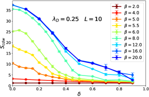
Figure 6: CDW structure factor versus hopping anisotropy $\delta$. The low temperature value of the CDW order parameter falls to approximately half of its isotropic value as $\delta\rightarrow 0.4$.

IV.3 Spectral Function

The spectral function can be obtained from the Green’s function measurement in DQMC combined with analytic continuation Jarrell and J.E.Gubernatis (1996) to invert the integral relation

$$G({\bf k},\tau)=\int d\omega\frac{A({\bf k},\omega)\ e^{-\tau\omega}}{e^{-\beta\omega}+1}$$ (6)

Following the procedure discussed in Ref. White, 1991, one can evaluate the moments

$$\mu_{1}({\bf k}) \equiv\int d\omega\,\omega\,A({\bf k},\omega)$$ (7)

$$=\big{(}\,\epsilon_{\bf k}-\mu\,)+\lambda\,\langle X\rangle$$

$$\mu_{2}({\bf k}) \equiv\int d\omega\,\omega^{2}\,A({\bf k},\omega)$$ (8)

$$=(\epsilon_{\mathbf{k}}-\mu)^{2}+2\lambda(\epsilon_{\mathbf{k}}-\mu)\langle X\rangle+\lambda^{2}\langle X^{2}\rangle$$

Here $\langle X\rangle$ is the phonon displacement on a spatial site, and is related to the density by $\langle X\rangle=-\lambda\langle n\rangle/\omega_{0}^{2}$. At half-filling, $\langle n\rangle=1$ and $\mu=U_{\rm eff}=-\lambda^{2}/\omega_{0}^{2}$ so that $\mu_{1}({\bf k})=\epsilon_{\bf k}$. (This is the same as for the noninteracting case, since there $A({\bf k},\omega)=\delta(\omega-\epsilon_{\bf k})$.) These analytic values of the moments, in combination with a measurement of the phonon potential energy, serve as a useful check on the analytic continuation. Preliminary tests indicate analytic continuation of the imaginary-time dependent Greens function obtained from DQMC yields values for the moments in agreement with the analytic results of Eq. (8) to within a few percent.

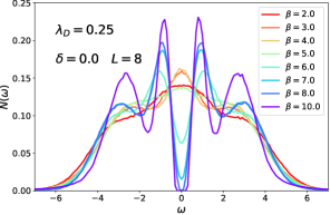
Figure 7: Density of states for the isotropic lattice for different inverse temperatures $\beta t$. The phonon frequency $\omega_{0}=t$ and electron-phonon coupling $g=\,t$. Finite size scaling of $S_{\rm cdw}$ suggests $\beta_{c}\,t=6.0\pm 0.1\,\,$ Costa et al. (2018), which is consistent with the $\beta$ value at which a full gap opens in $N(\omega)$.

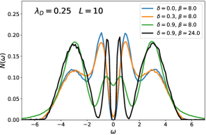
Figure 8: Density of states comparing the isotropic lattice with small ($\delta=0.3$) and large ($\delta=0.9$) anisotropy. For $\delta=0.9$ the opening of a gap is delayed until $\beta_{c}\,t\sim 20$.

Figure 7 shows the density of states $N(\omega)$ for the isotropic lattice. At inverse temperatures $\beta\,t=2,3,4,5$ (i.e. lower than $\beta_{c}t$), $N(\omega)$ has a peak at the Fermi level $\omega=0$. Beginning at the critical inverse temperature inferred from the finite size scaling of $S_{\rm cdw}$ Costa et al. (2018), $N(\omega)$ develops a gap, which provides another indication of the transition to the insulating CDW phase. Fig. 8 shows that $N(\omega)$ remains relatively unchanged under the influence of strain $\delta=0.3$, consistent with the robust $S_{\rm cdw}$ of Fig. 6 at modest anisotropy. However, at $\delta=0.9$ the CDW gap has been replaced by a weak minimum at $\beta\,t=8$ and is only recovered at $\beta\,t=24$.

The formation of a gap at $\delta=0.9$, even though the corresponding $S_{\rm cdw}$ value shown in Fig. 6 is small, is strong evidence that a CDW insulating phase persists out to very large $\delta$. It is useful to consider the two-dimensional Ising model when trying to understand this result. The Onsager solution gives a non-zero $T_{c}$ for all $J_{x}/J_{y}>0$ in the Ising model, a result consistent with the general expectation that anisotropy in the form of a weak coupling in one direction does not destroy a finite temperature second order phase transition in dimension $d$. The rough physical picture is that correlations will develop in the ‘strongly interacting’ directions out to a length $\xi$. The coordinated orientation of degrees of freedom in regions of size $\xi^{d-1}$ then creates a large ‘effective’ coupling $J_{\rm eff}\sim\xi^{d-1}J_{\rm small}$ in the weakly interacting direction. As $\xi$ grows, $J_{\rm eff}$ eventually boosts $J_{\rm small}$. This same argument can be applied to the CDW order in the Holstein model, a claim supported by Fig. 4 showing that for $T>T_{\rm cdw}$ density correlations first form in the direction of enhanced hopping.

V Discussion

In this work we investigated charge ordering in the Holstein model on a square lattice in the presence of anisotropic hopping, $t_{x},t_{y}=1-\delta,1+\delta$. For $\delta\lesssim 0.3$, the transition temperature $T_{\rm cdw}$ remains relatively stable, only decreasing significantly for $\delta\gtrsim 0.4$. However, both the electron kinetic energies and the structure factor $S_{\rm cdw}$ see significant shifts for small values of $\delta$. The suppression of $S_{\rm cdw}$, especially at larger strains, mirrors the smallness of the MFT order parameter $x_{1}$ with increasing $\delta$. Despite the smallness of $S_{\rm cdw}$ at low temperatures and large $\delta$, the opening of a gap in the density of states $N(\omega)$ at $\delta=0.90$ indicates the presence of an insulating CDW transition even as $\delta\rightarrow 1$.

While we have focused here exclusively on the effects of anisotropic electron hopping $t_{x}\neq t_{y}$ on charge correlations and the gap in the Holstein model, it is also possible to examine the role of changes in the phonon spectra. Indeed, DFT calculations Wei et al. (2017) indicate that such changes, e.g. enhancement of the phonon frequency with compression, are central to the onset of CDW order. Similarly, it is known from DQMC simulations that $T_{\rm cdw}$ exhibits a non-monotonic dependence on $\lambda_{D}=\lambda^{2}/(\omega_{0}^{2}\,W)$ in the Holstein Hamiltonian Zhang et al. (2019). The possibility of direct connection of such model calculations to materials would require the introduction of a connection of $\omega_{0}$ (and $\lambda$) to strain.

Applications of DQMC to Hamiltonians with repulsive electron-electron interactions are limited by the sign problem Loh et al. (1990); Troyer and Wiese (2005); study of Holstein or Su-Schrieffer-Heeger models with electron-phonon interactions are much less restricted. As seen here, and in other work Weber and Hohenadler (2018); Zhang et al. (2019); Chen et al. (2019), low enough temperatures can be reached to get a complete understanding of the CDW transition, and even of the possibility of quantum critical points Zhang et al. (2019); Chen et al. (2019) associated with CDW transitions driven by changes in $\lambda_{D}$ at $T=0$. Recent work has further exhibited this flexibility of DQMC by examining the effects of phonon dispersion on CDW order in the Holstein model Costa et al. (2018). In short, the freedom from the sign problem opens the door to incorporating additional materials details into quantum simulations of electron-phonon models and hence to the study of CDW transitions. Such rich details are much more difficult to include in studies of repulsive electron-electron interactions like the Hubbard model for which the sign problem is severe.

The density of states $N(\omega)$ gives information about the CDW gap. However, the momentum-resolved spectral function $A({\bf k},\omega)$ yields more detailed data concerning the effect of (strain) hopping anisotropy on the quasiparticle dispersion, and in particular, the possibility that gaps might develop at distinct temperatures as the momentum ${\bf k}$ changes. Work to study that possibility is in progress.

Acknowledgements: The work of B.C-S. and R.T.S. was supported by the Department of Energy under grant DE-SC0014671. N.C.C. was partially supported by the Brazilian funding agencies CAPES and CNPq. E.K. acknowledges support from the National Science Foundation (NSF) under Grant No. MR-1609560. Computations were performed in part on Spartan high-performance computing facility at San José State University, which is supported by the NSF under Grant No. OAC-1626645.

References

- Gan et al. (2016) L. Gan, L. Zhang, Q. Zhang, C. Guo, U. Schwingenschlogl, and Y. Zhao, Phys. Chem. Chem. Phys. 18, 3080 (2016).
- Wei et al. (2017) M. J. Wei, W. J. Lu, R. C. Xiao, H. Y. Lv, P. Tong, W. H. Song, and Y. P. Sun, Phys. Rev. B 96, 165404 (2017).
- Gao et al. (2018) S. Gao, F. Flicker, R. Sankar, H. Zhao, Z. Ren, B. Rachmilowitz, S. Balachandar, F. Chou, K. S. Burch, Z. Wang, J. van Wezel, and I. Zeljkovic, Proc. Nat. Acad. Sci. 115, 6986 (2018), https://www.pnas.org/content/115/27/6986.full.pdf .
- Johannes et al. (2006) M. D. Johannes, I. I. Mazin, and C. A. Howells, Phys. Rev. B 73, 205102 (2006).
- Johannes and Mazin (2008) M. D. Johannes and I. I. Mazin, Phys. Rev. B 77, 165135 (2008).
- Tsen et al. (2015) A. Tsen, R. Hovden, D. Wang, Y. Kim, J. Okamoto, K. Spoth, Y. Liu, W. Lu, Y. Sun, J. Hone, L. Kourkoutis, P. Kim, and A. Pasupathy, Proceedings of the National Academy of Sciences 112, 15054 (2015), https://www.pnas.org/content/112/49/15054.full.pdf .
- Yang et al. (2014) J. Yang, W. Wang, Y. Liu, H. Du, W. Ning, G. Zheng, C. Jin, Y. Han, N. Wang, Z. Yang, M. Tian, and Y. Zhang, Appl. Phys. Lett. 105, 063109 (2014).
- Renteria et al. (2014) J. Renteria, R. Samnakay, C. Jiang, T. Pope, P. Goli, Z.Yan, D. Wickramaratne, T. Salguero, A. Khitun, R. Lake, and A. Balandin, J. Appl. Phys. 115, 034305 (2014).
- Yu et al. (2015) Y. Yu, F. Yang, X. Lu, Y. Yan, Y. Cho, L. Ma, X. Niu, S. Kim, Y. Son, D. Feng, S. Li, S. Cheong, X. Chen, and Z. Y., Nat. Nanotechnol. 10, 270 (2015).
- Hollander et al. (2015) M. Hollander, Y. Liu, W. Lu, L. Li, Y. Sun, J. Robinson, and S. Datta, Nano Lett. 15, 1861 (2015).
- Samnakay et al. (2015) R. Samnakay, D. Wickramaratne, T. Pope, R. Lake, T. Salguero, and A. Balandin, Nano Lett. 15, 2965 (2015).
- Xi et al. (2015) X. Xi, L. Zhao, Z. Wang, H. Berger, L. Forró, J. Shan, , and K. Mak, Nat. Nanotech. 10, 765 (2015).
- Chen et al. (2015) P. Chen, Y. H. Chan, X. Fang, Y. Zhang, M. Y. Chou, S. K. Mo, Z. Hussain, A. V. Fedorov, and T. C. Chiang, Nat. Comm. 6, 8943 (2015).
- Chen et al. (2016) P. Chen, Y. Chan, M. Wong, X. Fang, M. Chou, S. Mo, Z. Hussain, A. Fedorov, and T. Chiang, Nano Lett. 16, 6331 (2016).
- Lian et al. (2017) C. Lian, C. Si, J. Wu, and W. Duan, Phys. Rev. B 96, 235426 (2017).
- Zhang et al. (2017) D. Zhang, J. Ha, H. Baek, Y.-H. Chan, F. D. Natterer, A. F. Myers, J. D. Schumacher, W. G. Cullen, A. V. Davydov, Y. Kuk, M. Y. Chou, N. B. Zhitenev, and J. A. Stroscio, Phys. Rev. Materials 1, 024005 (2017).
- Sengupta et al. (2002) P. Sengupta, A. W. Sandvik, and D. K. Campbell, Phys. Rev. B 65, 155113 (2002).
- Hirsch (1985) J. E. Hirsch, Phys. Rev. B 31, 4403 (1985).
- Iglovikov et al. (2015) V. I. Iglovikov, E. Khatami, and R. T. Scalettar, Phys. Rev. B 92, 045110 (2015).
- Holstein (1959) T. Holstein, Annals of Physics 8, 325 (1959).
- Su et al. (1979) W. Su, J. Schrieffer, and A. Heeger, Phys. Rev. Lett. 42, 1698 (1979).
- Costa et al. (2018) N. C. Costa, T. Blommel, W.-T. Chiu, G. Batrouni, and R. T. Scalettar, Phys. Rev. Lett. 120, 187003 (2018).
- Chen et al. (2019) C. Chen, X. Xu, Z. Meng, and M. Hohenadler, Phys. Rev. Lett. 122, 077601 (2019).
- Li et al. (2018) Z.-X. Li, M. L. Cohen, and D.-H. Lee, arXiv:1812.10263 (2018).
- Weber and Hohenadler (2018) M. Weber and M. Hohenadler, Phys. Rev. B 98, 085405 (2018).
- Zhang et al. (2019) X. Zhang, W. Chiu, N. Costa, G. Batrouni, and R. Scalettar, Phys. Rev. Lett. 122, 077602 (2019).
- Blankenbecler et al. (1981) R. Blankenbecler, D. J. Scalapino, and R. L. Sugar, Phys. Rev. D 24, 2278 (1981).
- White et al. (1989) S. R. White, D. J. Scalapino, R. L. Sugar, E. Y. Loh, J. E. Gubernatis, and R. T. Scalettar, Phys. Rev. B 40, 506 (1989).
- Gubernatis et al. (2016) J. Gubernatis, N. Kawashima, and P. Werner, Quantum Monte Carlo Methods: Algorithms for Lattice Models (Cambridge University Press, 2016).
- Assaad (2002) F. Assaad, in Quantum Simulations of Complex Many-Body Systems: From Theory to Algorithms, Vol. 10, edited by J. Grotendorst, D. Marx, and A. Muramatsu (NIC Series, 2002) pp. 99–156.
- dos Santos (2003) R. R. dos Santos, Brazilian Journal of Physics 33, 36 (2003).
- Loh et al. (1990) E. Loh, J. Gubernatis, R. Scalettar, S. White, D. Scalapino, and R. Sugar, Phys. Rev. B 41, 9301 (1990).
- Troyer and Wiese (2005) M. Troyer and U. Wiese, Phys. Rev. Lett. 94, 170201 (2005).
- Scalettar et al. (1991) R. T. Scalettar, R. M. Noack, and R. R. P. Singh, Phys. Rev. B 44, 10502 (1991).
- Batrouni and Scalettar (2018) G. G. Batrouni and R. T. Scalettar, arXiv:1808.08973 (2018).
- Jarrell and J.E.Gubernatis (1996) M. Jarrell and J.E.Gubernatis, Physics Reports 269, 133 (1996).
- White (1991) S. White, Phys. Rev. B 44, 4670 (1991).